chiral symmetry: an analytic $SU(3)$ unitary matrix

Abstract

The $SU(2)$ unitary matrix $U$ employed in chiral descriptions of hadronic low-energy processes has both exponential and analytic representations, related by $U=\exp\left[\,i\,\mbox{\boldmath$\tau$}\cdot\hat{\mbox{\boldmath$\pi$}}\,\theta\,\right]=\cos\theta\,I+i\,\mbox{\boldmath$\tau$}\cdot\hat{\mbox{\boldmath$\pi$}}\,\sin\theta$, where $\tau$ are Pauli matrices and $\mbox{\boldmath$\pi$}=(\pi_{1},\pi_{2},\pi_{3})$ is the pion field. One extends this result to the $SU(3)$ unitary matrix by deriving an analytic expression which, for Gell-Mann matrices $\lambda$, reads $U=\exp\left[\,i\,\mbox{\boldmath$v$}\cdot\mbox{\boldmath$\lambda$}\,\right]=\left[\,\left(F+\tfrac{2}{3}\,G\right)I+\left(H\,\hat{\mbox{\boldmath$v$}}+\tfrac{1}{\sqrt{3}}\,G\,\hat{\mbox{\boldmath$b$}}\right)\cdot\mbox{\boldmath$\lambda$}\,\right]+\,i\,\left[\,\left(Y+\tfrac{2}{3}\,Z\right)I+\left(X\,\hat{\mbox{\boldmath$v$}}+\tfrac{1}{\sqrt{3}}\,Z\,\hat{\mbox{\boldmath$b$}}\right)\cdot\mbox{\boldmath$\lambda$}\,\right]$, with $v_{i}=[\,v_{1},\cdots v_{8}\,]$, $b_{i}=d_{ijk}\,v_{j}\,v_{k}$, and factors $F,\cdots Z$ written in terms of elementary functions depending on $v=|\mbox{\boldmath$v$}|$ and $\eta=2\,d_{ijk}\,\hat{v}_{i}\,\hat{v}_{j}\,\hat{v}_{k}/3$. This result does not depend on the particular meaning attached to the variable $v$ and the analytic expression is used to calculate explicitly the associated left and right forms. When $v$ represents pseudoscalar meson fields, the classical limit corresponds to $\langle 0|\eta|0\rangle\rightarrow\eta\rightarrow 0$ and yields the cyclic structure $U=\left\{\left[\tfrac{1}{3}\left(1+2\,\cos v\right)\,I+\tfrac{1}{\sqrt{3}}\left(-1+\cos v\right)\,\hat{\mbox{\boldmath$b$}}\cdot\mbox{\boldmath$\lambda$}\right]+i\,\left(\sin v\right)\hat{\mbox{\boldmath$v$}}\cdot\mbox{\boldmath$\lambda$}\right\}$, which gives rise to a tilted circumference with radius $\sqrt{2/3}$ in the space defined by $I$, $\hat{\mbox{\boldmath$b$}}\cdot\mbox{\boldmath$\lambda$}$, and $\hat{\mbox{\boldmath$v$}}\cdot\mbox{\boldmath$\lambda$}$. For the sake of completeness, the axial transformations of the analytic matrix are also evaluated explicitly.

I motivation

The considerable progress in low-energy hadron physics achieved over the last sixty years is closely associated with chiral symmetry. Quantum chromodynamics (QCD), the present-day strong theory, involves gluons and six quarks with different flavors, which have color. Direct applications to low-energy processes are very difficult owing to gluon–gluon interactions and one has to resort to either lattice methodsLattQCD or effective descriptions. The latter depart from the symmetries of QCD, namely the continuous Poincaré group, discrete C, P and T inversions, together electric charge and baryon number conservation. The quark masses $m_{q}$ are external parameters and the lightest ones, $m_{u}$, $m_{d}$, and $m_{s}$, can be considered as small in the scale $\Lambda\sim 1\,\mathrm{GeV}$. This rationale underlies the idea of chiral symmetry, an approximate scheme that becomes exact in the ideal limit $m_{q}\rightarrow 0$. In this case, helicity is a good quantum number and the quark fields $q$ are written as linear combinations of $q_{R}$ and $q_{L}$, with spins respectively parallel and anti-parallel to their momenta. As helicity is conserved in interactions, the fields $q_{R}$ and $q_{L}$ do not couple and the Lagrangian is symmetric under the chiral group $U(N)_{R}\times U(N)_{L}$, where N is the number of flavors. However, owing to the the $U(1)_{A}$ anomaly, the actual group to be considered is $U(1)_{V}\times SU(3)_{R}\times SU(3)_{L}$. In effective descriptions, these symmetries of QCD are associated directly with hadronic degrees of freedom, bypassing quarks and gluons.

The incorporation of chiral symmetry into hadron physics precedes QCD and was already being discussed in 1960. A long-lasting contribution from that year is the idea that the strong vacuum is not empty, presented by Gell-Mann and LévyGellMannLevy in a paper introducing both linear and non-linear $\sigma$-models for pions and nucleons. The former relied on the $\sigma$, a scalar particle proposed earlier by SchwingerSchwinger , and provided a unique tool for dealing with the strong vacuum. In the symmetric version, the model involves just two parameters, usually denoted by $\mu$ and $\lambda$, whose values determine whether the ground state of the theory is either empty or contains a classical component, associated with a condensate. Almost simultaneously, in 1961, Nambu and Jona-LasinioNambuJonaL studied the strong vacuum employing an alternative chiral model inspired by superconductivity, which also involved a scalar-isoscalar state. Their model was based on fermionic fields, the pion being a collective state, and contained a vacuum phase transition described by a gap-equation, controlled by a free parameter. A common feature of both models is the indication that chiral symmetry allows the ground state of strong systems to be realized in two different ways, namely: (i) the Wigner–Weyl mode, in which states with opposite parities are degenerate and the vacuum is empty; (ii) the Nambu–Goldstone mode, in which the pion is a massless Goldstone boson, the scalar state is massive and the vacuum contains a condensate. Also in 1961, Skyrme succeeded in describing baryons as topological solitons composed of chiral pions, carrying a well defined quantum numberSkyrme . He employed classical pion fields constrained by a non-linear condition and assumed the proton to be a deformation of the strong vacuum, kept stable for topological reasons. Nowadays, these states are known as skyrmions but, at the time, they were criticized for not having spin and deserved little attention. However, about two decades later, spins were incorporated into the model by Adkins, Nappi and WittenAdNaWit , and its rich structure could be properly appreciated.

After QCD became established as the strong theory, applications of chiral symmetry were aimed mostly at improving the precision of predictions and nowadays chiral perturbation theory (ChPT) is employed to tackle low-energy hadronic processes. This research program was outlined by Weinberg in 1979Weinberg1 and fully developed by Gasser and Leutwyler for the SU(2) sector in 1984GassLeut1 . Low-energy interactions are strongly dominated by quarks $u$ and $d$ and their small masses are treated as perturbations into a massless $SU(2)\times SU(2)$ symmetric Lagrangian involving effective pion fields. ChPT is a well-defined theory and allows the systematic expansion of low-energy amplitudes in powers of a typical scale $q\sim M_{\pi}<1\,\mathrm{GeV}$. Nevertheless, while QCD is fully renormalizable, ChPT can only be renormalized order by orderWeinberg1 . The effective lagrangian consists of strings of terms possessing the most general structure consistent with broken chiral symmetry and both its form and the number of low-energy constants (LECs) associated with renormalization depend on the order considered.

All approaches to strong interactions mentioned, namely the models produced by Gell-Mann and Lévy, Nambu and Jona-Lasinio, and Skyrme, together with ChPT, did bring important progress to the area. With hindsight, however, one realizes that all of them have specific limitations and none has superseded completely the others. So, in spite of their differences, they coexist and the relevance of each one depends on the particular problem considered. A common feature of these competing strategies is that, in all cases, early works were performed in the framework of $SU(2)$ for reasons of simplicity. The basic unitary $SU(2)$ matrix $U$ can be represented as

$$U=\exp\left[\,i\,\mbox{\boldmath$\tau$}\cdot\hat{\mbox{\boldmath$\pi$}}\,\theta\,\right]\;,\hskip 14.22636pt\rightarrow\;\;\mathrm{exponential}\;\mathrm{representation}$$ (1)

where $\hat{\mbox{\boldmath$\pi$}}$ is the direction of the pion field in isospin space and $\theta$ is the chiral angle. As it is well known, the series implicit in the exponential can be summed and one gets the equivalent form

$$U=\cos\theta\,I+i\,\mbox{\boldmath$\tau$}\cdot\hat{\mbox{\boldmath$\pi$}}\,\sin\theta\;,\hskip 14.22636pt\rightarrow\;\;\mathrm{analytic}\;\mathrm{representation}$$ (2)

which one calls analytic, in the want of a better name. It is employed in the non-linear $\sigma$-model and suited to comparisons with the linear version, based on the non-unitary matrix

$$M=\sigma\,I+i\,\mbox{\boldmath$\tau$}\cdot\mbox{\boldmath$\pi$}\;.$$ (3)

The simplicity of these structures facilitates comparisons among different schemes and allows one to study the mathematical reasons behind their main features.

The various approaches have been generalized to $SU(3)$ and this version of the $\sigma$-modelLevy employs a matrix $M$ composed by nonets of pseudoscalar and scalar states, whereas the extended version of ChPT relies on the exponential formGassLeut2 . In the case of the Skyrme model, the $SU(3)$ group is employed just in the quantization of the soliton, which is carried out formallyChemtob ; ChemtobBlaizot . The conceptual mobility among these generalizations to $SU(3)$ is more difficult than in $SU(2)$, partly owing to the absence of a suitable analytic expression for the matrix $U$ which could provide a bridge among them. Analytic results based on Euler angles already exist for this matrix Nelson ; AkyRas ; Byrd and find applications in many areas of physics dealing with three state systems, such as color superconductivitycolor , opticsoptics , geometric phasesgeompha , and quantum entanglement in computation and communicationentanglement . However, Euler angles require a set of external axes and are inconvenient to applications of chiral symmetry to low-energy processes. In sect.II one derives an alternative analytic representation for the matrix $U$, written in terms of internal degrees of freedom and corresponding to an extension of eq.(2). In hadron physics, this result may be instrumental to simplifying calculations and studying topological properties of $SU(3)$, for both flavor and color, in analogy to the case of the skyrmion. The unitarity of $U$ in analytic form is explored in sect.III and the corresponding left and right forms are presented in sect.IV. Its classical limit is discussed in sect.V, chiral transformations of are given in sect.VI, conclusions are summarized in sect.VII, and technical matters are presented in four appendices.

II analytic form

The exponential form of $U$ in $SU(3)$ is written in terms of the Gell-Mann matrices $\mbox{\boldmath$\lambda$}=[\,\lambda_{1},\cdots\lambda_{8}\,]$, satisfying $\left[\lambda_{i},\lambda_{j}\right]=2\,i\,f_{ijk}\,\lambda_{k}$ and $\left\{\lambda_{i},\lambda_{j}\right\}=\tfrac{4}{3}\,\delta_{ij}\,I+2\,d_{ijk}\,\lambda_{k}$, coupled with a generic octet $\mbox{\boldmath$v$}=[\,v_{1},\cdots v_{8}\,]$ as

$$U=\exp\left[\,i\,\mbox{\boldmath$v$}\cdot\mbox{\boldmath$\lambda$}\,\right]$$

$$\hskip 14.22636pt=\left[1-\frac{v^{2}}{2!}\left[\hat{\mbox{\boldmath$v$}}\cdot\mbox{\boldmath$\lambda$}\right]^{2}+\cdots\right]+i\,\left[\frac{v}{1!}\left[\hat{\mbox{\boldmath$v$}}\cdot\mbox{\boldmath$\lambda$}\right]-\frac{v^{3}}{3!}\left[\hat{\mbox{\boldmath$v$}}\cdot\mbox{\boldmath$\lambda$}\right]^{3}+\cdots\right]$$ (4)

with $\mbox{\boldmath$v$}\cdot\mbox{\boldmath$\lambda$}=v_{i}\,\lambda_{i}$, $v=\sqrt{v_{i}\,v_{i}}$, and $\hat{\mbox{\boldmath$v$}}=\mbox{\boldmath$v$}/v$.

One uses two auxiliary variables in the derivation of the analytic form. One of them is the bilinear construct $\mbox{\boldmath$b$}=[\,b_{1},\cdots b_{8}\,]$,

$$b_{i}=d_{ijk}\,v_{j}\,v_{k}\;,$$ (5)

with $b=\sqrt{\,b_{i}\,b_{i}}=v^{2}/\sqrt{3}$ and $\hat{\mbox{\boldmath$b$}}=\mbox{\boldmath$b$}/b$. The other is

$$\eta=\frac{2}{3\,v^{3}}\;D=\frac{2}{3\,\sqrt{3}}\;\hat{\mbox{\boldmath$v$}}\cdot\hat{\mbox{\boldmath$b$}}\;,$$ (6)

where $D=\mbox{\boldmath$v$}\cdot\mbox{\boldmath$b$}=d_{ijk}\,v_{i}\,v_{j}\,v_{k}$. The quantity $b$ is even under $\mbox{\boldmath$v$}\rightarrow-\mbox{\boldmath$v$}$, $\eta$ is odd, and the latter is a measure of the overlap between $b$ and $v$. As $\hat{\mbox{\boldmath$v$}}$ and $\hat{\mbox{\boldmath$b$}}$ are unit vectors, $|\hat{\mbox{\boldmath$v$}}\cdot\hat{\mbox{\boldmath$b$}}|\leq 1$, and $\eta$ lies in the interval $-\tfrac{2}{3\,\sqrt{3}}\leq\eta\leq\tfrac{2}{3\,\sqrt{3}}$. The explicit forms of $b_{i}$ and $D$ are given in App.A and shown to satisfy the conditions

$$f_{ijk}\,v_{j}\,b_{k}=0\;,$$ (7)

$$d_{ijk}\,v_{j}\,b_{k}=\tfrac{1}{3}\,v^{2}\,v_{i}\;,$$ (8)

$$d_{ijk}\,b_{j}\,b_{k}=\eta\,v^{3}\,v_{i}-\tfrac{1}{3}\,v^{2}\,b_{i}\;,$$ (9)

which allow one to write

$$\left[\,\hat{\mbox{\boldmath$v$}}\cdot\mbox{\boldmath$\lambda$}\,\right]\,\left[\hat{\mbox{\boldmath$v$}}\cdot\mbox{\boldmath$\lambda$}\,\right]=\tfrac{2}{3}\,I+\tfrac{1}{\sqrt{3}}\;\hat{\mbox{\boldmath$b$}}\cdot\mbox{\boldmath$\lambda$}\;,$$ (10)

$$\left[\,\hat{\mbox{\boldmath$v$}}\cdot\mbox{\boldmath$\lambda$}\,\right]\,\left[\hat{\mbox{\boldmath$v$}}\cdot\mbox{\boldmath$\lambda$}\,\right]\,\left[\hat{\mbox{\boldmath$v$}}\cdot\mbox{\boldmath$\lambda$}\,\right]=\hat{\mbox{\boldmath$v$}}\cdot\mbox{\boldmath$\lambda$}+\eta\,I\;.$$ (11)

In order to simplify the notation, one defines

$$A=\hat{\mbox{\boldmath$v$}}\cdot\mbox{\boldmath$\lambda$}\;,$$ (12)

$$B=\tfrac{2}{3}\,I+\tfrac{1}{\sqrt{3}}\;\hat{\mbox{\boldmath$b$}}\cdot\mbox{\boldmath$\lambda$}\;,$$ (13)

so that

$$A^{2}=AA=B\;,$$ (14)

$$A^{3}=AB=A+\eta\,I\;,$$ (15)

$$A^{4}=AAB=BB=B+\eta\,A\;.$$ (16)

Thus, $A^{5}=A\left(B+\eta\,A\right)=A+\eta\,I+\eta\,B$, and so on. These results mean that, in matrix space, $U$ is a linear combinations of $I$, $A$ and $B$. The matrices $I$ and $B$ are even under $\mbox{\boldmath$v$}\rightarrow-\mbox{\boldmath$v$}$, whereas $A$ is odd.

The matrix $U$ is written as

$$U=\sum_{n=0}^{\infty}i^{n}\,\frac{v^{n}}{{n}!}\,A^{n}=U_{\mathrm{even}}+i\,U_{\mathrm{odd}}\;,$$ (17)

where the labels even and odd refer to $\mbox{\boldmath$v$}\rightarrow-\mbox{\boldmath$v$}$, and one has

$$\frac{\partial U_{\text{even}}}{\partial v}=-A\,U_{\text{odd}}\;,$$ (18)

$$\frac{\partial U_{\text{odd}}}{\partial v}=A\,U_{\text{even}}\;.$$ (19)

In matrix space, one writes

$$U_{\text{even}}=\sum_{n=0}^{\infty}(i)^{2n}\frac{v^{2n}}{(2n)!}\left[\,f_{2n}\,I+g_{2n}\,B+h_{2n}\,A\,\right]$$

$$\hskip 17.07164pt=F(v,\eta)\,I+G(v,\eta)\,B+H(v,\eta)\,A\;,$$ (20)

$$U_{\text{odd}}=\sum_{n=0}^{\infty}(i)^{2n}\frac{v^{2n+1}}{(2n+1)!}\left[\,x_{2n+1}\,A+y_{2n+1}\,I+z_{2n+1}\,B\,\right]$$

$$\hskip 19.91692pt=X(v,\eta)\,A+Y(v,\eta)\,I+Z(v,\eta)\,B\;,$$ (21)

where the functions $F,G,H,X,Y,\mathrm{and}\,Z$ are determined in the sequence. In tables 1 and 2, one displays a few partial contributions to these series and it is possible to note that the dependences on $v$ and $\eta$ do not mix. Even and odd components are related by the action of the matrix A, which yields

$$A\,\left[\,f_{2n}\,I+g_{2n}\,B+h_{2n}\,A\,\right]=\left[\,(f_{2n}+g_{2n})\,A+\eta\,g_{2n}\,I+h_{2n}\,B\,\right]$$

$$\hskip 14.22636pt=\left[\,x_{2n+1}\,A+y_{2n+1}\,I+z_{2n+1}\,B\,\right]\;,$$ (22)

$$A\,\left[\,x_{2n+1}\,A+y_{2n+1}\,I+z_{2n+1}\,B\,\right]=\left[\,\eta\,z_{2n+1}\,I+x_{2n+1}\,B+(y_{2n+1}+z_{2n+1})\,A\,\right]$$

$$\hskip 14.22636pt=\left[\,f_{2n+2}\,I+g_{2n+2}\,B+h_{2n+2}\,A\,\right]\;.$$ (23)

n	$(i\,v)^{n}/n!$	$f_{n}\,(\times I)$	$g_{n}\,(\times B)$	$h_{n}\,(\times A)$
0	1	1
2	$-v^{2}/2!$		1
4	$v^{4}/4!$		1	$\eta$
6	$-v^{6}/6!$	$\eta^{2}$	1	$2\eta$
8	$v^{8}/8!$	$2\,\eta^{2}$	$1+\eta^{2}$	$3\,\eta$
10	$-v^{10}/10!$	$3\,\eta^{2}$	$1+3\,\eta^{2}$	$4\,\eta+\eta^{3}$
12	$v^{12}/12!$	$4\,\eta^{2}+\eta^{4}$	$1+6\,\eta^{2}$	$5\,\eta+4\,\eta^{3}$
14	$-v^{14}/14!$	$5\,\eta^{2}+4\,\eta^{4}$	$1+10\,\eta^{2}+\eta^{4}$	$6\,\eta+10\,\eta^{3}$
16	$v^{16}/16!$	$6\,\eta^{2}+10\,\eta^{4}$	$1+15\,\eta^{2}+5\,\eta^{4}$	$7\,\eta+20\,\eta^{3}+\eta^{5}$

Table 1: Structure of $U_{\text{even}}$, eq.(20).

n	$(i\,v)^{n}/n!$	$x_{n}\,(\times A)$	$y_{n}\,(\times I)$	$z_{n}\,(\times B)$
1	$i\,v$	1
3	$-i\,v^{3}/3!$	1	$\eta$
5	$i\,v^{5}/5!$	1	$\eta$	$\eta$
7	$-i\,v^{7}/7!$	$1+\eta^{2}$	$\eta$	$2\,\eta$
9	$i\,v^{9}/9!$	$1+3\,\eta^{2}$	$\eta+\eta^{3}$	$3\,\eta$
11	$-i\,v^{11}/11!$	$1+6\,\eta^{2}$	$\eta+3\,\eta^{3}$	$4\,\eta+\eta^{3}$
13	$i\,v^{13}/13!$	$1+10\,\eta^{2}+\eta^{4}$	$\eta+6\,\eta^{3}$	$5\,\eta+4\,\eta^{3}$
15	$-i\,v^{15}/15!$	$1+15\,\eta^{2}+5\,\eta^{4}$	$\eta+10\,\eta^{3}+\eta^{5}$	$6\,\eta+10\,\eta^{3}$
17	$i\,v^{17}/17!$	$1+21\,\eta^{2}+15\,\eta^{4}$	$\eta+15\,\eta^{3}+5\,\eta^{5}$	$7\,\eta+20\,\eta^{3}+\eta^{5}$

Table 2: Structure of $i\,U_{\text{odd}}$, eq.(21).

Using results (18)-(21), one writes

$$\frac{\partial}{\partial v}\left[F\,I+G\,B+H\,A\right]=-\left[\eta\,Z\,I+X\,B+(Y+Z)A\right]\;,$$ (24)

$$\frac{\partial}{\partial v}\left[X\,A+Y\,I+Z\,B\right]=\left[\left(F+G\right)A+\eta\,I+H\,B\right]\;.$$ (25)

and obtains a set of first order differential equations coupling even and odd components

$$\frac{\partial F}{\partial v}=-\eta\,Z\;,\hskip 34.1433pt\frac{\partial G}{\partial v}=-X\;,\hskip 34.1433pt\frac{\partial H}{\partial v}=-Y-Z\;,$$ (26)

$$\frac{\partial X}{\partial v}=F+G\;,\hskip 28.45274pt\frac{\partial Y}{\partial v}=\eta\,G\;,\hskip 36.98857pt\frac{\partial Z}{\partial v}=H\;.$$ (27)

A further derivation decouples these sectors, yielding

$$\frac{\partial^{2}F}{\partial v^{2}}=-\eta\,H\;,\hskip 45.5244pt\frac{\partial^{2}G}{\partial v^{2}}=-F-G\;,\hskip 28.45274pt\frac{\partial^{2}H}{\partial v^{2}}=-\eta\,G-H\;,$$ (28)

$$\frac{\partial^{2}X}{\partial v^{2}}=-\eta\,Z-X\;,\hskip 22.76219pt\frac{\partial^{2}Y}{\partial v^{2}}=-\eta\,X\;,\hskip 42.67912pt\frac{\partial^{2}Z}{\partial v^{2}}=-Y-Z\;.$$ (29)

In order to get an uncoupled differential equation for $F$, one increases the number of derivatives and finds

$$\frac{\partial^{6}F}{\partial v^{6}}+2\,\frac{\partial^{4}F}{\partial v^{4}}+\frac{\partial^{2}F}{\partial v^{2}}+\eta^{2}\,F=0\;.$$ (30)

Its general solution is discussed in App.B and given by

$$F=\beta_{1}\,\cos(k_{1}\,v)+\beta_{2}\,\cos(k_{2}\,v)+\beta_{3}\,\cos(k_{3}\,v)\;,$$ (31)

where $\beta_{i}$ are constants and, using the results of App.B, one has

$$k_{i}=\tfrac{2}{\sqrt{3}}\,\sin(\theta/6+\delta_{i}\,\pi/3)\;,$$ (32)

$$\cos(\theta)=1-27\,\eta^{2}/2\;,\hskip 14.22636pt\sin(\theta)=3\sqrt{3}\,\eta\,\sqrt{1-27\,\eta^{2}/4}\;,$$ (33)

and $\delta_{1}=0,\delta_{2}=1,\delta_{3}=-1$.

The constants $\beta_{i}$ are fixed by expanding $\cos(k_{i}\,v)$ in series and, expressing results in terms of the roots $\alpha_{i}=-k_{i}^{2}$ of the cubic equation $\alpha_{i}^{3}+2\,\alpha_{i}^{2}+\alpha_{i}+\eta^{2}=0$, eq.(119), one has

$$F=(\beta_{1}+\beta_{2}+\beta_{3})+\frac{v^{2}}{2!}\,(\beta_{1}\,\alpha_{1}+\beta_{2}\,\alpha_{2}+\beta_{3}\,\alpha_{3})+\frac{v^{4}}{4!}\,(\beta_{1}\,\alpha_{1}^{2}+\beta_{2}\,\alpha_{2}^{2}+\beta_{3}\,\alpha_{3}^{2})$$

$$\hskip 14.22636pt+\frac{v^{6}}{6!}\,\sum\beta_{i}\,\alpha_{i}^{3}+\frac{v^{8}}{8!}\,\sum\beta_{i}\,\alpha_{i}^{4}+\,\frac{v^{10}}{10!}\,\sum\beta_{i}\,\alpha_{i}^{5}+\frac{v^{12}}{12!}\,\sum\beta_{i}\,\alpha_{i}^{6}+\cdots\;.$$ (34)

Comparing results for $v^{0}$, $v^{2}$ and $v^{4}$ with those of table 1, one learns that

$$\beta_{1}+\beta_{2}+\beta_{3}=1\;,$$ (35)

$$\beta_{1}\,\alpha_{1}+\beta_{2}\,\alpha_{2}+\beta_{3}\,\alpha_{3}=0\;,$$ (36)

$$\beta_{1}\,\alpha_{1}^{2}+\beta_{2}\,\alpha_{2}^{2}+\beta_{3}\,\alpha_{3}^{2}=0\;.$$ (37)

Terms proportional to powers of $v$ $\geq 6$ are evaluated using combinations of eqs.(35)-(37) and (119). Thus, for instance

$$\sum\beta_{i}\,\alpha_{i}^{3}=\sum\,\beta_{i}\left[-2\,\alpha_{i}^{2}-\alpha_{i}-\eta^{2}\right]=-\eta^{2}\;,$$ (38)

$$\sum\beta_{i}\,\alpha_{i}^{4}=\sum\,\beta_{i}\,\alpha_{i}\,\left[-2\,\alpha_{i}^{2}-\alpha_{i}-\eta^{2}\right]=2\,\eta^{2}\;,$$ (39)

$$\sum\beta_{i}\,\alpha_{i}^{5}=\sum\,\beta_{i}\,\alpha_{i}^{2}\,\left[-2\,\alpha_{i}^{2}-\alpha_{i}-\eta^{2}\right]=-3\,\eta^{2}\;,$$ (40)

$$\sum\beta_{i}\,\alpha_{i}^{6}=\sum\,\beta_{i}\,\left[-2\,\alpha_{i}^{2}-\alpha_{i}-\eta^{2}\right]^{2}=4\,\eta^{2}+\eta^{4}\;.$$ (41)

Using these results into eq.(31), one has

$$F=1-\frac{v^{6}}{6!}\,\eta^{2}+\frac{v^{8}}{8!}\,2\,\eta^{2}-\frac{v^{10}}{10!}\,3\,\eta^{2}+\frac{v^{12}}{12!}\,\left(4\,\eta^{2}+\eta^{4}\right)+\cdots$$ (42)

and the entry in table 1 is reproduced.

Expressions (35)-(37) yield directly

$$\beta_{i}=-\,\frac{\alpha_{j}\,\alpha_{k}}{(\alpha_{i}-\alpha_{j})\,(\alpha_{k}-\alpha_{i})}\;,$$ (43)

with $[i,j,k]\rightarrow\mathrm{cyclic}\;\mathrm{permutations}\;\mathrm{of}\;[1,2,3]$. Alternative versions are useful in calculations and, employing condition (119), on has

$$\beta_{i}=\frac{\eta^{2}}{\alpha_{i}\,(\alpha_{i}-\alpha_{j})\,(\alpha_{k}-\alpha_{i})}\;.$$ (44)

The denominator can be simplified using results of App.B and one finds the set of alternatives

$$\beta_{i}=\frac{\eta^{2}}{2\,(\alpha_{i}^{2}+\alpha_{i})+3\,\eta^{2}}\;,$$ (45)

$$\beta_{i}=-\,\frac{\eta^{2}}{(\alpha_{i}^{2}+\alpha_{i})\,(3\,\alpha_{i}+1)}\;,$$ (46)

$$\beta_{i}=\frac{\alpha_{i}+1}{(3\,\alpha_{i}+1)}\,.$$ (47)

The last expression determines the condition

$$\sum_{i}\frac{1}{(3\,\alpha_{i}+1)}=0\;.$$ (48)

Result (31) for $F$ and eqs.(26)-(29) determine the set of functions $G$, $H$, $X$, $Y$, and $Z$. Choosing form (47) for the $\beta_{i}$, one has

$$F=\frac{(\alpha_{1}+1)}{(3\,\alpha_{1}+1)}\;\cos(k_{1}\,v)+[1\rightarrow 2,3]\;,$$ (49)

$$G=-\,\frac{1}{(3\,\alpha_{1}+1)}\;\cos(k_{1}\,v)+[1\rightarrow 2,3]\;,$$ (50)

$$H=\frac{\eta}{(\alpha_{1}+1)\,(3\,\alpha_{1}+1)}\;\cos(k_{1}\,v)+[1\rightarrow 2,3]\;,$$ (51)

$$X=-\,\frac{1}{(3\,\alpha_{1}+1)}\;k_{1}\sin(k_{1}\,v)+[1\rightarrow 2,3]\;,$$ (52)

$$Y=\frac{\eta}{\alpha_{1}\,(3\,\alpha_{1}+1)}\;k_{1}\sin(k_{1}\,v)+[1\rightarrow 2,3]\;,$$ (53)

$$Z=-\,\frac{\eta}{\alpha_{1}\,(\alpha_{1}+1)\,(3\,\alpha_{1}+1)}\;k_{1}\sin(k_{1}\,v)+[1\rightarrow 2,3]\;.$$ (54)

The parity of these functions under $\mbox{\boldmath$v$}\rightarrow-\mbox{\boldmath$v$}$ is determined by $\eta$ and therefore $F$, $G$, and $X$ are even, whereas $H$, $Y$, and $Z$ are odd.

The analytic form of the matrix $U$, derived from eqs.(20) and (21), reads

$$U=\left(F\,I+G\,B+H\,A\right)+i\left(Y\,I+Z\,B+X\,A\right)\;,$$ (55)

$$\hskip 11.38109pt=\left[\,\left(F+\tfrac{2}{3}\,G\right)\,I+\left(H\,\hat{\mbox{\boldmath$v$}}+\tfrac{1}{\sqrt{3}}\,G\,\hat{\mbox{\boldmath$b$}}\right)\cdot\mbox{\boldmath$\lambda$}\,\right]$$

$$\hskip 11.38109pt+\,i\,\left[\,\left(Y+\tfrac{2}{3}\,Z\right)\,I+\left(X\,\hat{\mbox{\boldmath$v$}}+\tfrac{1}{\sqrt{3}}\,Z\,\hat{\mbox{\boldmath$b$}}\right)\cdot\mbox{\boldmath$\lambda$}\,\right]\;.$$ (56)

As there is an overlap between $\hat{\mbox{\boldmath$v$}}$ and $\hat{\mbox{\boldmath$b$}}$, one might consider replacing the latter by the unit vector $\hat{\mbox{\boldmath$u$}}$ given by

$$\hat{\mbox{\boldmath$b$}}=\frac{3\,\sqrt{3}}{2}\,\eta\,\hat{\mbox{\boldmath$v$}}+\sqrt{1-\frac{27\,\eta^{2}}{4}}\,\hat{\mbox{\boldmath$u$}}\;,$$ (57)

such that $\hat{\mbox{\boldmath$v$}}\cdot\hat{\mbox{\boldmath$u$}}=0$. However, this is not especially useful.

In order to deal with a more compact expression, one defines the quantities

$$S=\left(F+\tfrac{2}{3}\,G\right)\;,\hskip 42.67912ptQ_{i}=\sqrt{\tfrac{2}{3}}\,\left(H\,\hat{v}_{i}+\tfrac{1}{\sqrt{3}}\,G\,\hat{b}_{i}\right)\;,$$ (58)

$$W=\left(Y+\tfrac{2}{3}\,Z\right)\;,\hskip 42.67912ptP_{i}=\sqrt{\tfrac{2}{3}}\,\left(X\,\hat{v}_{i}+\tfrac{1}{\sqrt{3}}\,Z\,\hat{b}_{i}\right)\;,$$ (59)

and expresses the equivalence between exponential and analytic representations as

$$U=\exp\left[\,i\,\mbox{\boldmath$v$}\cdot\mbox{\boldmath$\lambda$}\,\right]=\left[\,S\,I+\sqrt{\tfrac{3}{2}}\,\mbox{\boldmath$Q$}\cdot\mbox{\boldmath$\lambda$}\,\right]+i\,\left[\,W\,I+\sqrt{\tfrac{3}{2}}\,\mbox{\boldmath$P$}\cdot\mbox{\boldmath$\lambda$}\,\right]\;.$$ (60)

III unitarity

The matrix $U$ satisfies the $SU(3)$ conditions $U^{\dagger}\,U=I$ and $\text{det}\,U=1$ irrespective of the representation adopted, as ensured by result (60). Nevertheless, it is useful to explore the unitarity condition expressed in analytic form given by eqs.(55) and (56), since it gives rise to constraints among the factors $F,\cdots Z$. Explicit multiplication using form (55), together with eqs.(14)-(16), yields

$$U^{\dagger}\,U=C_{I}\,I+C_{B}\,B+C_{A}\,A\;,$$ (61)

with

$$C_{I}=F^{2}+2\,\eta\,GH+Y^{2}+2\,\eta\,XZ\;,$$ (62)

$$C_{B}=G^{2}+H^{2}+2\,FG+X^{2}+Z^{2}+2\,YZ\;,$$ (63)

$$C_{A}=\eta\,G^{2}+2\,FH+2\,GH+\eta\,Z^{2}+2\,XY+2\,XZ\;,$$ (64)

and, in App.C, one shows that

$$C_{I}=1\;,\hskip 28.45274ptC_{B}=0\;,\hskip 28.45274ptC_{A}=0\;.$$ (65)

Alternatively, form (60) gives rise to

$$U^{\dagger}\,U=\left[S^{2}+Q^{2}+W^{2}+P^{2}\,\right]I$$

$$\hskip 14.22636pt+\left\{\sqrt{6}\,SQ_{k}+\tfrac{3}{2}\,Q_{i}Q_{j}\,d_{ijk}+\sqrt{6}\,WP_{k}+\tfrac{3}{2}\,P_{i}P_{j}\,d_{ijk}+\tfrac{3}{2}\,Q_{i}P_{j}\,f_{ijk}\right\}\lambda_{k}\;.$$ (66)

Definitions (58), (59), with results (5), (8) and (9), allow one to show that the term within curly brackets is

$$\left\{\cdots\right\}=C_{A}\,\hat{v}_{k}+\tfrac{1}{\sqrt{3}}\,C_{B}\,\hat{b}_{k}=0\;.$$ (67)

Writing

$$Q^{2}=Q_{i}\,Q_{i}=\tfrac{2}{9}\,G^{2}+\tfrac{2}{3}\,H^{2}+2\,\eta\,GH\;,$$ (68)

$$P^{2}=P_{i}\,P_{i}=\tfrac{2}{3}\,X^{2}+\tfrac{2}{9}\,Z^{2}\,+2\,\eta\,XZ\;,$$ (69)

one also has

$$U^{\dagger}\,U=\left[S^{2}+Q^{2}+W^{2}+P^{2}\,\right]I$$

$$\hskip 14.22636pt=\left[F^{2}+\tfrac{4}{3}\,FG+\tfrac{2}{3}\,G^{2}+\tfrac{2}{3}\,H^{2}+2\,\eta\,GH\right.$$

$$\left.\hskip 14.22636pt+\,Y^{2}+\tfrac{4}{3}\,YZ+\tfrac{2}{3}\,Z^{2}+\tfrac{2}{3}\,X^{2}+2\,\eta\,XZ\,\right]I$$

$$\hskip 14.22636pt=\left[C_{I}+\tfrac{2}{3}\,C_{B}\right]I=I\;.$$ (70)

This means that

$$U^{\dagger}\,U=I\rightarrow S^{2}+Q^{2}+W^{2}+P^{2}=1\;,$$ (71)

indicating that the variables $S,Q,W,P$ are constrained to the surface of a four-dimensional sphere, irrespective of the values of the free parameters $v$ and $\eta$. This is relevant for applications of chiral symmetry to low-energy strong systems, which involve both vector and axial transformations. In $SU(3)$, the former promote changes in the labels of $Q_{i}$ and $P_{i}$ while keeping $Q=\pm\sqrt{Q_{i}\,Q_{i}}$ and $P=\pm\sqrt{P_{i}\,P_{i}}$ invariant. The latter, on the other hand, modify all functions $S,Q,W,P$ together and the constraint imposed by unitarity corresponds to a generalization of the $SU(2)$ condition $\sigma^{2}+\pi^{2}=\text{constant}$ of the non-linear $\sigma$-modelGellMannLevy . The dependence of the functions $S^{2}$, $Q^{2}$, $W^{2}$, and $P^{2}$ on $v$ is displayed in fig.1, where full and dashed curves correspond to $\eta=0$ and the arbitrary value $\eta=1/\sqrt{54}=0.1361$, respectively. As expected from the explicit results for $F,\cdots Z$ in eqs.(49)-(54), just the case $\eta=0$ yields cyclic structures. It is worth noting that, in this case, the odd scalar term $W$ vanishes.

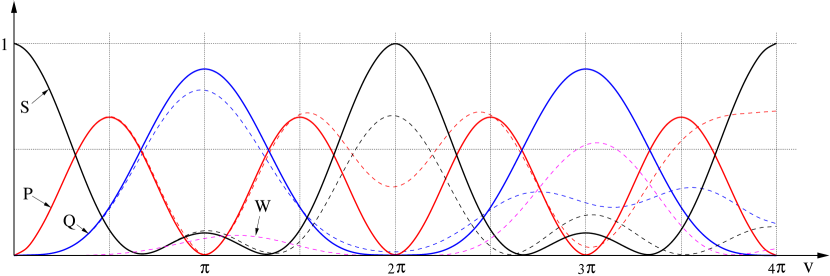
Figure 1: $S^{2}$, $Q^{2}$, $W^{2}$ and $P^{2}$ as functions of $v$ for $\eta=0$ (continuous curves) and $\eta=0.1361$ (dashed curves).

The situation in $SU(3)$ contrasts with the $SU(2)$ case, where the variation of the chiral angle $\theta$ gives rise to oscillations of scalar and pseudoscalar variables constrained to a circle. Denoting the trace by $\langle\cdots\rangle$, one shows in fig.2 the behaviour of the components $S^{2}+Q^{2}=\tfrac{1}{3}\langle U_{\text{even}}^{2}\rangle$ and $(W^{2}+P^{2})=\tfrac{1}{3}\langle U_{\text{odd}}^{2}\rangle$ as functions of $v$, for $\eta=0$ and $\eta=0.1361$. In the case $\eta=0$ one has $W=0$ and these functions oscillate, with values restricted to the intervals $1\geq\left(S^{2}+Q^{2}\right)\geq 1/3$ and $2/3\geq P^{2}\geq 0$. The idividual scalar contributions $S^{2}$ and $Q^{2}$ do vanish at specific points, but their sum does not. This interplay between $S$ and $Q$ within the even sector is a distinctive feature of the $SU(3)$ case.

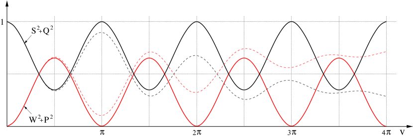
Figure 2: $\left(S^{2}+Q^{2}\right)$ and $\left(W^{2}+P^{2}\right)$ as functions of $v$ for $\eta=0$ (continuous curves) and $\eta=0.1361$ (dashed curves); note that $(S^{2}+Q^{2})+(W^{2}+P^{2})=1$, as in eq.(71).

IV left and right forms

The analytic result for $U$, eq.(60), allows one to derive the left and right forms $L^{\mu}$ and $R^{\mu}$, defined by

$$L^{\mu}=U^{\dagger}\,\frac{\partial U}{\partial x^{\mu}}\;,\hskip 28.45274ptR^{\mu}=U\,\frac{\partial U^{\dagger}}{\partial x^{\mu}}\;.$$ (72)

They are related to the vector and axial currents $V^{\mu}$ and $A^{\mu}$ by

$$L^{\mu}=i\,\left(V^{\mu}-A^{\mu}\right)\;,\hskip 28.45274ptR^{\mu}=i\,\left(V^{\mu}+A^{\mu}\right)$$ (73)

and, owing to the unitarity condition $U^{\dagger}\,U=I$, one has

$$[L^{\mu}]^{\dagger}=-L^{\mu}\,,\hskip 28.45274pt[R^{\mu}]^{\dagger}=-R^{\mu}\;.$$ (74)

The left form is evaluated in App.D and reads

$$L^{\mu}=i\,\left\{\tfrac{3}{2}\left[\left(Q_{i}\,\partial^{\mu}Q_{j}+P_{i}\,\partial^{\mu}P_{j}\right)f_{ijk}\right]\right.$$

$$\hskip 14.22636pt\left.+\,\left[\sqrt{\tfrac{3}{2}}\left(\,S\,\partial^{\mu}P_{k}-P_{k}\,\partial^{\mu}S-W\,\partial^{\mu}Q_{k}+Q_{k}\,\partial^{\mu}W\right)\right.\right.$$

$$\hskip 14.22636pt\left.\left.+\tfrac{3}{2}\left(Q_{i}\,\partial^{\mu}P_{j}-P_{i}\,\partial^{\mu}Q_{j}\,\right)d_{ijk}\right]\right\}\lambda_{k}\;.$$ (75)

Writing $L^{\mu}=i\,\left(V_{k}^{\mu}-A_{k}^{\mu}\right)\lambda_{k}$, eqs.(191) and (193) allow one to express the currents in terms of the basic functions $F,\cdots,Z$ as

$$V_{k}^{\mu}=\left[\left(H^{2}+X^{2}\right)\,\hat{v}_{i}\,\partial^{\mu}\hat{v}_{j}+\,\tfrac{1}{\sqrt{3}}\left(G\,H+X\,Z\right)\left(\hat{v}_{i}\,\partial^{\mu}\hat{b}_{j}+\hat{b}_{i}\,\partial^{\mu}\hat{v}_{j}\right)\right.$$

$$\hskip 14.22636pt\left.+\,\tfrac{1}{3}\left(G^{2}+Z^{2}\right)\,\hat{b}_{i}\,\partial^{\mu}\hat{b}_{j}\right]f_{ijk}\;,$$ (76)

$$A_{k}^{\mu}=-\left\{\left[1\right]\hat{v}_{k}\,\partial^{\mu}v\right.$$

$$\left.+\,\frac{1}{(1-\tfrac{27}{4}\eta^{2})}\left[\left(GY-FZ\right)+\tfrac{9}{4}\eta\left(FX-HY\right)\right.\right.$$

$$\left.\left.+\,\tfrac{3}{4}\eta\left(HZ-GX\right)-\tfrac{9}{4}\,v\,\eta\right]\hat{v_{k}}\,\partial^{\mu}\eta\right.$$

$$\left.+\,\frac{1}{(1-\tfrac{27}{4}\eta^{2})}\,\tfrac{1}{\sqrt{3}}\left[\tfrac{3}{2}\left(HY-FX\right)+\tfrac{1}{2}\left(GX-HZ\right)\right.\right.$$

$$\left.\left.+\,\tfrac{9}{2}\eta\left(FZ-GY\right)+\tfrac{3}{2}\,v\right]\hat{b}_{k}\,\partial^{\mu}\eta\right.$$

$$\left.+\left[\left(F+\tfrac{2}{3}G\right)X-H\left(Y+\tfrac{2}{3}Z\right)\right]\partial^{\mu}\hat{v}_{k}\right.$$

$$\left.+\,\tfrac{1}{\sqrt{3}}\left[\left(F+\tfrac{2}{3}G\right)Z-G\left(Y+\tfrac{2}{3}Z\right)\right]\partial^{\mu}\hat{b}_{k}\right.$$

$$\left.+\tfrac{1}{\sqrt{3}}\left(HZ-GX\right)\left(\hat{v}_{i}\,\partial^{\mu}\hat{b}_{j}-\hat{b}_{i}\,\partial^{\mu}\hat{v}_{j}\right)d_{ijk}\right\}\;.$$ (77)

V classical limit

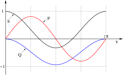
Figure 3: Classical $S$, $Q$ and $P$ as functions of $v$.

In the case of spontaneous symmetry breaking, the variable $v$ may acquire a non-vanishing vacuum expectation value and become the $SU(3)$ analogous of the $SU(2)$ chiral angle $\theta$. As the same does not apply for $\eta$, which has odd parity under $\mbox{\boldmath$v$}\rightarrow-\mbox{\boldmath$v$}$, one referers to the situation $\langle 0|v|0\rangle\neq 0$ and $\eta\rightarrow 0$ as the classical limit. In this case, one has

$$k_{1}\rightarrow\eta\hskip 14.22636pt\rightarrow\hskip 14.22636pt\alpha_{1}\rightarrow-\eta^{2}\;,$$ (78)

$$k_{2,3}\rightarrow\pm 1+\frac{\eta}{2}\hskip 14.22636pt\rightarrow\hskip 14.22636pt\alpha_{2,3}\rightarrow-(1\pm\eta)\;,$$ (79)

and finds

$$F\rightarrow 1\;,$$ (80)

$$G\rightarrow-1+\cos v\;,$$ (81)

$$X\rightarrow\sin v\;,$$ (82)

whereas $H,Y,Z\rightarrow{\cal O}(\eta)$.

Figure 4: Projections of the classical circle (in red) over planes (a) $PQ$, (b) $QS$, and (c) $SP$; figure (b) shows the profile of the circle over the plane associated with $U_{\text{even}}$, whereas figures (a) and (c) are obtained by rotating it by $\pi/2$ along axes $Q$ and $S$ respectively; in all figures, the axis not shown points out of the page.

In the classical limit $W\rightarrow 0$ and the behavior of the functions

$$S\rightarrow\tfrac{1}{3}\,\left(1+2\,\cos v\right)\;,$$ (83)

$$Q\rightarrow\tfrac{\sqrt{2}}{3}\,\left(-1+\cos v\right)\;,$$ (84)

$$P\rightarrow\sqrt{\tfrac{2}{3}}\,\sin v\;,$$ (85)

is shown in fig.3 and the matrix $U$ becomes

$$U=\left[\tfrac{1}{3}\left(1+2\,\cos v\right)\,I+\tfrac{1}{\sqrt{3}}\,\left(-1+\cos v\right)\,\hat{\mbox{\boldmath$b$}}\cdot\mbox{\boldmath$\lambda$}\right]+i\,\left(\sin v\right)\hat{\mbox{\boldmath$v$}}\cdot\mbox{\boldmath$\lambda$}\;.$$ (86)

The unitarity condition (71) constrains $S$, $Q$ and $P$ to the surface of a sphere, since

$$U^{\dagger}\,U=I\rightarrow S^{2}+Q^{2}+P^{2}=1\;,$$ (87)

and the variation of $v$ gives rise to a circumference, with projections over planes $PQ$, $QS$, and $SP$ shown in fig.4. Figure $(b)$, depicting the two components of $U_{\text{even}}$, is particularly interesting, for it shows the profile of a circle as a straight line, for eqs.(83) and (84) yield

$$S=1-\sqrt{2}\,Q\;.$$ (88)

Thus, the path determined by $v$ is tilted circumference, defined by the intersection of the unit sphere with a plane orthogonal to the axes $Q$ and $S$, inclined by an angle $\epsilon=\tan^{-1}\sqrt{2}$, which amounts to $\sin\epsilon=\sqrt{2/3}$, $\cos\epsilon=\sqrt{1/3}$, and $\epsilon\sim 54.76^{\circ}$. Performing a rotation around the $P$ axis, as in fig.5, one has

$$S^{\prime}=\sqrt{\tfrac{1}{3}}\,S-\sqrt{\tfrac{2}{3}}\,Q\;,\hskip 42.67912ptQ^{\prime}=\sqrt{\tfrac{2}{3}}\,S+\sqrt{\tfrac{1}{3}}\,Q\;,$$ (89)

and the equation of the plane containing the circle is $S^{\prime}=\sqrt{1/3}$. Its edge is determined by condition (87), which now reads $Q^{{}^{\prime}2}+P^{2}=1-S^{{}^{\prime}2}=2/3$, corresponding to a radius of $\sqrt{2/3}$ and to $Q^{\prime}=\sqrt{2/3}\,\cos v$.

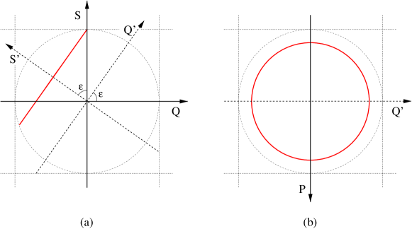
Figure 5: Projections of the classical circle (in red) over planes (a) $Q^{\prime}S^{\prime}$ and (b) $Q^{\prime}P$; in both figures, the axis not shown points out of the page.

VI chiral symmetry

One now concentrates on the case of pseudoscalar mesons $\phi$ and, making $\mbox{\boldmath$v$}\rightarrow\mbox{\boldmath$\phi$}$, discusses the chiral transformations of the matrix $U(\mbox{\boldmath$\phi$})$ given by eq.(60). Its vector transformations are associated with changes in the directions of $\hat{\mbox{\boldmath$\phi$}}$ and $\hat{\mbox{\boldmath$b$}}$ and need not be written out explicitly. Concerning axial tranformations $\delta^{A}\mbox{\boldmath$\phi$}$, the most general non-linear form has been discussed by WeinbergWeinberg68 and is given by

$$\delta^{A}\phi_{a}=f^{A}(\phi^{2})\,\beta_{a}+g^{A}(\phi^{2})\,\beta_{i}\,\phi_{i}\,\phi_{a}\;,$$ (90)

where $\beta_{i}$ are free parameters, $f^{A}$ is an arbitrary function and

$$g^{A}=\frac{2f^{A}f^{{}^{\prime}A}+1}{f^{A}-2\,\phi^{2}f^{{}^{\prime}A}}\;,$$ (91)

with $f^{{}^{\prime}A}=df^{A}/d\phi^{2}$. The axial transformation of a generic function $\psi(v,\eta)$ is

$$\delta^{A}\psi=\frac{d\psi}{d\phi_{a}}\,\delta^{A}\phi_{a}=\left[\frac{\partial\psi}{\partial\phi}\,\hat{\phi}_{a}+\frac{\partial\psi}{\partial\eta}\,\frac{1}{\phi}\left(-3\eta\,\hat{\phi_{a}}+\frac{2}{\sqrt{3}}\,\hat{b}_{a}\right)\right]\delta^{A}\phi_{a}\;,$$ (92)

using eq.(183). Evaluating the derivatives of $(F,\cdots Z)$ with the help of eqs.(26), (27) and (164)-(169), one has

$$\delta^{A}F=\frac{1}{1-\tfrac{27}{4}\eta^{2}}\left\{\left[\frac{1}{\phi}\left(9\,\eta^{2}G-3\,\eta H\right)+\left(\tfrac{9}{2}\,\eta^{2}X-3\,\eta Y-\eta Z\right)\right]\hat{\phi}_{a}\right.$$

$$\hskip 22.76219pt\left.+\frac{2}{\sqrt{3}}\left[\frac{1}{\phi}\left(-3\,\eta G+H\right)+\left(-\tfrac{3}{2}\,\eta X+Y+\tfrac{9}{4}\,\eta^{2}Z\right)\right]\hat{b}_{a}\right\}\delta^{A}\phi_{a}\;,$$ (93)

$$\delta^{A}G=\frac{1}{1-\tfrac{27}{4}\eta^{2}}\left\{\left[\frac{1}{\phi}\left(-\tfrac{27}{2}\,\eta^{2}G+\tfrac{9}{2}\,\eta H\right)+\left(-X+\tfrac{9}{2}\,\eta Y+\tfrac{3}{2}\,\eta Z\right)\right]\hat{\phi}_{a}\right.$$

$$\hskip 22.76219pt\left.+\frac{2}{\sqrt{3}}\left[\frac{1}{\phi}\left(\tfrac{9}{2}\,\eta G-\tfrac{3}{2}\,H\right)+\left(\tfrac{9}{4}\,\eta X-\tfrac{3}{2}\,Y-\tfrac{1}{2}\,Z\right)\right]\hat{b}_{a}\right\}\delta^{A}\phi_{a}\;,$$ (94)

$$\delta^{A}H=\frac{1}{1-\tfrac{27}{4}\eta^{2}}\left\{\left[\frac{1}{\phi}\left(3\,\eta G-\tfrac{27}{4}\,\eta^{2}H\right)+\left(\tfrac{3}{2}\,\eta X-Y-Z+\tfrac{9}{2}\,\eta^{2}Z\right)\right]\hat{\phi}_{a}\right.$$

$$\hskip 22.76219pt\left.+\frac{2}{\sqrt{3}}\left[\frac{1}{\phi}\left(-G+\tfrac{9}{4}\,\eta H\right)+\left(-\tfrac{1}{2}\,X+\tfrac{9}{4}\,\eta Y+\tfrac{3}{4}\,\eta Z\right)\right]\hat{b}_{a}\right\}\delta^{A}\phi_{a}\;,$$ (95)

$$\delta^{A}X=\frac{1}{1-\tfrac{27}{4}\eta^{2}}\left\{\left[\frac{1}{\phi}\left(-\tfrac{27}{4}\,\eta^{2}X+3\,\eta Z\right)+\left(F+G-\tfrac{9}{2}\,\eta^{2}G-\tfrac{3}{2}\,\eta H\right)\right]\hat{\phi}_{a}\right.$$

$$\hskip 22.76219pt\left.+\frac{2}{\sqrt{3}}\left[\frac{1}{\phi}\left(\tfrac{9}{4}\,\eta X-Z\right)+\left(-\tfrac{9}{4}\,\eta F-\tfrac{3}{4}\,\eta G+\tfrac{1}{2}\,H\right)\right]\hat{b}_{a}\right\}\delta^{A}\phi_{a}\;,$$ (96)

$$\delta^{A}Y=\frac{1}{1-\tfrac{27}{4}\eta^{2}}\left\{\left[\frac{1}{\phi}\left(-3\,\eta X+9\,\eta^{2}Z\right)+\left(3\,\eta F+\eta G-\tfrac{9}{2}\,\eta^{2}H\right)\right]\hat{\phi}_{a}\right.$$

$$\hskip 22.76219pt\left.+\frac{2}{\sqrt{3}}\left[\frac{1}{\phi}\left(X-3\,\eta Z\right)+\left(-F-\tfrac{9}{4}\,\eta^{2}G+\tfrac{3}{2}\,\eta H\right)\right]\hat{b}_{a}\right\}\delta^{A}\phi_{a}\;,$$ (97)

$$\delta^{A}Z=\frac{1}{1-\tfrac{27}{4}\eta^{2}}\left\{\left[\frac{1}{\phi}\left(\tfrac{9}{2}\,\eta X-\tfrac{27}{2}\,\eta^{2}Z\right)+\left(-\tfrac{9}{2}\,\eta F-\tfrac{3}{2}\,\eta G+H\right)\right]\hat{\phi}_{a}\right.$$

$$\hskip 22.76219pt\left.+\frac{2}{\sqrt{3}}\left[\frac{1}{\phi}\left(-\tfrac{3}{2}\,X+\tfrac{9}{2}\,\eta Z\right)+\left(\tfrac{3}{2}\,F+\tfrac{1}{2}\,G-\tfrac{9}{4}\,\eta H\right)\right]\hat{b}_{a}\right\}\delta^{A}\phi_{a}\;,$$ (98)

whereas the two directions transform as

$$\delta^{A}\,\hat{\phi}_{i}=\frac{1}{\phi}\left(\delta_{ia}-\hat{\phi}_{i}\,\hat{\phi}_{a}\right)\,\delta^{A}\phi_{a}\;,$$ (99)

$$\delta^{A}\,\hat{b}_{i}=\frac{2\sqrt{3}}{\phi}\left(d_{ija}\,\hat{\phi}_{j}-\tfrac{1}{\sqrt{3}}\,\hat{b}_{i}\,\hat{\phi}_{a}\right)\,\delta^{A}\phi_{a}\;.$$ (100)

One notes that, as expected, axial transformations change the parities of the functions $F,\cdots,Z$, and of the directions $\hat{\mbox{\boldmath$\phi$}}$ and $\hat{\mbox{\boldmath$b$}}$, under the operation $\mbox{\boldmath$\phi$}\rightarrow-\mbox{\boldmath$\phi$}$.

Using results (93)-(98) one can, for instance, show that the functions $C_{I}$, $C_{B}$ and $C_{A}$ given by eqs.(62)-(63) are invariant under axial transformations by means of explicit calculations. In the case of classical fields, these transformations become much simpler and read

$$\delta^{A}F=0\hskip 14.22636pt\rightarrow\hskip 14.22636pt\delta^{A}1=0\;,$$ (101)

$$\delta^{A}G=-X\,\hat{\phi}_{a}\,\delta^{A}\phi_{a}\hskip 14.22636pt\rightarrow\hskip 14.22636pt\delta^{A}\left(-1+\cos\phi\right)=-\sin\phi\,\delta^{A}\phi\;,$$ (102)

$$\delta^{A}X=\left(F+G\right)\hat{\phi}_{a}\,\delta^{A}\phi_{a}\hskip 14.22636pt\rightarrow\hskip 14.22636pt\delta^{A}\sin\phi=\cos\phi\,\delta^{A}\phi\;$$ (103)

using $\hat{\phi}_{a}\,\delta^{A}\phi_{a}=\delta^{A}\phi$. Thus, the axial transformation implements a rotation along the tilted circumference discussed in sect.V.

VII summary

One presents an analytic expression for the $SU(3)$ unitary matrix which, although motivated by low-energy hadron physiscs, has a more general validity.

1. The $SU(2)$ unitary matrix $U$ is well known to have two equivalent representations, given by $U=\exp\left[\,i\,\mbox{\boldmath$\tau$}\cdot\hat{\mbox{\boldmath$\pi$}}\,\theta\,\right]=\cos\theta+i\,\mbox{\boldmath$\tau$}\cdot\hat{\mbox{\boldmath$\pi$}}\,\sin\theta$, where $\tau$ are Pauli matrices and $\mbox{\boldmath$\pi$}=(\pi_{1},\pi_{2},\pi_{3})$ is the pion field. In sect.II one extends this result to the $SU(3)$ case and, for Gell-Mann matrices $\lambda$, derives the identity

$$U=\exp\left[\,i\,\mbox{\boldmath$v$}\cdot\mbox{\boldmath$\lambda$}\,\right]=\left[\,S\,I+\sqrt{\tfrac{3}{2}}\,\mbox{\boldmath$Q$}\cdot\mbox{\boldmath$\lambda$}\,\right]+i\,\left[\,W\,I+\sqrt{\tfrac{3}{2}}\,\mbox{\boldmath$P$}\cdot\mbox{\boldmath$\lambda$}\,\right]\;,$$

with $(S+iW)=\left[(F+iY)+\tfrac{2}{3}\,(G+iZ)\right]$, $(Q+iP)_{i}=\sqrt{\tfrac{2}{3}}\,\left[(H+iX)\,\hat{v}_{i}+\tfrac{1}{\sqrt{3}}\,(G+iZ)\,\hat{b}_{i}\right]$, $v_{i}=[\,v_{1},\cdots v_{8}\,]$, $b_{i}=d_{ijk}\,v_{j}\,v_{k}$, and functions $F,\cdots,Z$ given by eqs.(49)-(54), depending on $v=|\mbox{\boldmath$v$}|$ and $\eta=2\,d_{ijk}\,\hat{v}_{i}\,\hat{v}_{j}\,\hat{v}_{k}/3$.

2. Unitarity constrains the functions $S,Q=\pm\sqrt{Q_{i}Q_{i}},\,W,P=\pm\sqrt{P_{i}P_{i}}$ to the surface of a four-sphere, since

$$U^{\dagger}\,U=I\rightarrow S^{2}+Q^{2}+W^{2}+P^{2}=1\;,$$

for all values of $v$ and $\eta$.

3. The analytic result for $U$ allows the explicit evaluation of the left form, which reads

$$L^{\mu}=i\,\left\{\tfrac{3}{2}\left[\left(Q_{i}\,\partial^{\mu}Q_{j}+P_{i}\,\partial^{\mu}P_{j}\right)f_{ijk}\right]\right.$$

$$\hskip 14.22636pt\left.+\,\left[\sqrt{\tfrac{3}{2}}\left(\,S\,\partial^{\mu}P_{k}-P_{k}\,\partial^{\mu}S-W\,\partial^{\mu}Q_{k}+Q_{k}\,\partial^{\mu}W\right)\right.\right.$$

$$\hskip 14.22636pt\left.\left.+\tfrac{3}{2}\left(Q_{i}\,\partial^{\mu}P_{j}-P_{i}\,\partial^{\mu}Q_{j}\,\right)d_{ijk}\right]\right\}\lambda_{k}\;.$$

This gives rise to the right form as well as to vector and axial currents. In sect.IV, one presents expressions in terms of the functions $F,\cdots Z$, which can be used in calculations.

4. In the classical limit, corresponding to $\eta\rightarrow 0$ and $\langle 0|v|0\rangle\neq 0$, one has $W\rightarrow 0$ and obtains the simpler form

$$U=\left[\,S\,I+\sqrt{\tfrac{3}{2}}\,Q\,\hat{\mbox{\boldmath$b$}}\cdot\mbox{\boldmath$\lambda$}\,\right]+i\,\sqrt{\tfrac{3}{2}}\,P\,\hat{\mbox{\boldmath$v$}}\cdot\mbox{\boldmath$\lambda$}\;,$$ (104)

with $S\rightarrow\tfrac{1}{3}\,\left(1+2\,\cos v\right)$, $Q\rightarrow\tfrac{\sqrt{2}}{3}\,\left(-1+\cos v\right)$ and $P\rightarrow\sqrt{\tfrac{2}{3}}\,\sin v$, satisfying $S^{2}+Q^{2}+P^{2}=1$. The matrix $U$ becomes a cyclic function of $v$ and oscillates, but its even and odd components under $\mbox{\boldmath$v$}\rightarrow-\mbox{\boldmath$v$}$ remain restricted to the intervals $1\geq(S^{2}+Q^{2})\geq 1/3$ and $2/3\geq P^{2}\geq 0$, as indicated in fig.2. The variation of $v$ determines a tilted circumference with radius $\sqrt{2/3}$ in the space defined by $I$, $\hat{\mbox{\boldmath$b$}}\cdot\mbox{\boldmath$\lambda$}$, and $\hat{\mbox{\boldmath$v$}}\cdot\mbox{\boldmath$\lambda$}$, illustrated in fig.4. In terms of the variable $Q^{\prime}=2\,S/\sqrt{3}+Q/\sqrt{3}$, its edge is given by $Q^{{}^{\prime}2}+P^{2}=2/3$ and, in the case of chiral symmetry, this corresponds to a generalization of the condition $\sigma^{2}+\pi^{2}=\text{constant}$ of the non-linear $SU(2)$ $\sigma$-model.

5. In sect.VI, the generic analytic expression for $U$ is adapted to low-energy flavor $SU(3)$ by associating the $v_{i}$ with pseudoscalar fields $\phi_{i}$ and one displays its axial transformation properties, involving both the functions $F,\cdots Z$ and the directions $\hat{\mbox{\boldmath$\phi$}}$ and $\hat{\mbox{\boldmath$b$}}$. In the classical limit, one has $\delta^{A}\cos\phi=-\sin\phi\,\delta^{A}\phi$ and $\delta^{A}\sin\phi=\cos\phi\,\delta^{A}\phi$, indicating that the axial transformation corresponds to a rotation along the tilted circumference.

6. Results given in sects.II, III and IV are generic and not committed to a particular interpretation of the variable $v$. Hence, they may prove to be useful in problems involving three degrees of freedom or three state systems. In QCD, one has the lightest flavors $u,d,s$ and the basic colors, where it might be instrumental either to study color superconductivity or to investigate topological properties of the classical solution, as in the Skyrme model. The interest of the analytic form of $U$ is not restricted to hadron physics and it may also be applied in other areas, such as optics, geometric phases, quantum computation, and communication.

Appendix A auxiliary functions

The explicit components of the vector $b$ are given by

$$b_{1}=\tfrac{2}{\sqrt{3}}\,v_{1}\,v_{8}+v_{4}\,v_{6}+v_{5}\,v_{7}\;,$$ (105)

$$b_{2}=\tfrac{2}{\sqrt{3}}\,v_{2}\,v_{8}-v_{4}\,v_{7}+v_{5}\,v_{6}\;,$$ (106)

$$b_{3}=\tfrac{2}{\sqrt{3}}v_{3}\,v_{8}+\tfrac{1}{2}\,\left(v_{4}^{2}+v_{5}^{2}-v_{6}^{2}-v_{7}^{2}\right)\;,$$ (107)

$$b_{4}=v_{1}\,v_{6}-v_{2}\,v_{7}+v_{3}\,v_{4}-\tfrac{1}{\sqrt{3}}\,v_{4}\,v_{8}\;,$$ (108)

$$b_{5}=v_{1}\,v_{7}+v_{2}\,v_{6}+v_{3}\,v_{5}-\tfrac{1}{\sqrt{3}}\,v_{5}\,v_{8}\;,$$ (109)

$$b_{6}=v_{1}\,v_{4}+v_{2}\,v_{5}-v_{3}\,v_{6}-\tfrac{1}{\sqrt{3}}\,v_{6}\,v_{8}\;,$$ (110)

$$b_{7}=v_{1}\,v_{5}-v_{2}\,v_{4}-v_{3}\,v_{7}-\tfrac{1}{\sqrt{3}}\,v_{7}\,v_{8}\;,$$ (111)

$$b_{8}=\tfrac{1}{\sqrt{3}}\left[\,v_{1}^{2}+v_{2}^{2}+v_{3}^{2}-\tfrac{1}{2}\left(v_{4}^{2}+v_{5}^{2}+v_{6}^{2}+v_{7}^{2}\right)-v_{8}^{2}\right]\;,$$ (112)

whereas the function $D$ reads

$$D=d_{ijk}\,v_{i}\,v_{j}\,v_{k}$$

$$=\sqrt{3}\,\left[\,v_{1}^{2}+v_{2}^{2}+v_{3}^{2}-\tfrac{1}{2}\left(v_{4}^{2}+v_{5}^{2}+v_{6}^{2}+v_{7}^{2}\right)-\tfrac{1}{3}\,v_{8}^{2}\,\right]\,v_{8}$$

$$+\;3\,v_{1}\left(\,v_{4}\,v_{6}+v_{5}\,v_{7}\,\right)+3\,v_{2}\left(\,-v_{4}\,v_{7}+v_{5}\,v_{6}\,\right)+\tfrac{3}{2}\,v_{3}\left(\,v_{4}^{2}+v_{5}^{2}-v_{6}^{2}-v_{7}^{2}\right)\;.$$ (113)

Using Jacobi identitiesGasio , one shows that the components of $b$ satisfy the conditions

$$f_{ijk}\,v_{j}\,b_{k}=0\;,$$ (114)

$$d_{jks}\,v_{j}\,b_{k}=\tfrac{1}{3}\,v^{2}\,v_{i}\;.$$ (115)

Alternatively, it is straightforward to prove these results by using directly eqs.(105)-(112). Multiplying eq.(115) by $b_{i}$, one finds $b^{2}=v^{4}/3$. Also, using $B\,B=B+\eta\,A$, eq.(16), one has $(\hat{b}\cdot\lambda)\,(\hat{b}\cdot\lambda)=2/3+3\,\eta\,\hat{v}\cdot\lambda-\hat{b}\cdot\lambda/\sqrt{3}$, which yields

$$d_{ijk}\,b_{j}\,b_{k}=\eta\,v^{3}\,v_{i}-\tfrac{1}{3}\,v^{2}\,b_{i}\;.$$ (116)

Appendix B differential equation

One considers the differential equation (30), that reads

$$\frac{\partial^{6}F}{\partial v^{6}}+2\,\frac{\partial^{4}F}{\partial v^{4}}+\frac{\partial^{2}F}{\partial v^{2}}+\eta^{2}\,F=0\;.$$ (117)

Its solution has the general form $F=\exp(q\,v)$ , where $q$ satisfies the algebraic equation

$$q^{6}+2\,q^{4}+q^{2}+\eta^{2}=0\;.$$ (118)

Defining $\alpha=q^{2}$, one has the cubic equation

$$\alpha^{3}+2\,\alpha^{2}+\alpha+\eta^{2}=0\;,$$ (119)

which has the solutions

$$\alpha_{1}=q_{1}^{2}=-\tfrac{2}{3}\left[\,1-\cos(\theta/3)\,\right]\;,$$ (120)

$$\alpha_{2}=q_{2}^{2}=-\tfrac{2}{3}\left[\,1-\cos(\theta/3+2\pi/3)\,\right]\;,$$ (121)

$$\alpha_{3}=q_{3}^{2}=-\tfrac{2}{3}\left[\,1-\cos(\theta/3-2\pi/3)\,\right]\;,$$ (122)

with

$$\cos(\theta)=1-27\,\eta^{2}/2\;,$$ (123)

$$\sin(\theta)=3\sqrt{3}\,\eta\,\sqrt{1-27\,\eta^{2}/4}\;.$$ (124)

As $\alpha_{i}<0$, one defines $q_{i}=i\,k_{i}$, and has

$$k_{1}=\tfrac{2}{\sqrt{3}}\,\sin(\theta/6)\;,$$ (125)

$$k_{2}=\tfrac{2}{\sqrt{3}}\,\sin(\theta/6+\pi/3)=\cos(\theta/6)+\tfrac{1}{\sqrt{3}}\,\sin(\theta/6)\;,$$ (126)

$$k_{3}=\tfrac{2}{\sqrt{3}}\,\sin(\theta/6-\pi/3)=-\cos(\theta/6)+\tfrac{1}{\sqrt{3}}\,\sin(\theta/6)\;.$$ (127)

The function $F$ is real and its most general form reads

$$F=\beta_{1}\,\cos(k_{1}\,v)+\beta_{2}\,\cos(k_{2}\,v)+\beta_{3}\,\cos(k_{3}\,v)\;,$$ (128)

where the $\beta_{i}$ are constants.

The $k_{i}$ satisfy the constraints

$$k_{1}=k_{2}+k_{3}\;,$$ (129)

$$k_{1}^{2}+k_{2}^{2}+k_{3}^{2}=2\;,$$ (130)

$$k_{1}\,k_{2}\,k_{3}=-\eta\;,$$ (131)

whereas, for the roots of the cubic equation (119) one has the usual conditions

$$\alpha_{1}+\alpha_{2}+\alpha_{3}=-2\;,$$ (132)

$$\alpha_{1}\,\alpha_{2}+\alpha_{2}\,a_{3}+\alpha_{3}\,\alpha_{1}=1\;,$$ (133)

$$\alpha_{1}\,\alpha_{2}\,\alpha_{3}=-\eta^{2}\;,$$ (134)

Combining (132) and (133), one finds the useful result

$$\alpha_{i}^{2}+2\,\alpha_{i}+\alpha_{j}^{2}+2\,\alpha_{j}+\alpha_{i}\,\alpha_{j}+1=0\;,$$ (135)

that can also be rewritten as

$$(\alpha_{i}^{2}+\alpha_{i})+(\alpha_{j}^{2}+\alpha_{j})=-(\alpha_{i}+1)\,(\alpha_{j}+1)\;.$$ (136)

Multiplying it by $\alpha_{i}$ and using (119), one gets

$$\alpha_{i}^{2}\,\alpha_{j}+2\,\alpha_{i}\,\alpha_{i}+\alpha_{i}\,\alpha_{j}^{2}-\eta^{2}=\alpha_{i}\,\alpha_{j}\,\left(\,2+\alpha_{i}+\alpha_{j}\,\right)-\eta^{2}=0$$ (137)

and, using (135) and (137), one also shows that

$$(\alpha_{i}^{2}+\alpha_{i})\,(\alpha_{j}^{2}+\alpha_{j})=\eta^{2}\,(1+\alpha_{i}+\alpha_{j})\;.$$ (138)

Appendix C unitarity - proof

The unitarity of the matrix $U$ is indicated in eq.(61) and here one proves the validity of conditions (65). Using the shorthands $c_{i}=\cos(k_{i}\,v)$ and $s_{i}=\sin(k_{i}\,v)$ in eqs.(49)-(54) and results from App.B, one has

$$F^{2}=\left\{\beta_{1}^{2}c_{1}^{2}\,[1]+2\beta_{1}\beta_{2}c_{1}c_{2}\,[1]+\cdots\right\}\;,$$ (139)

$$G^{2}=\frac{1}{\eta^{2}}\left\{\beta_{1}^{2}c_{1}^{2}\,[-\alpha_{1}]+2\beta_{1}\beta_{2}c_{1}c_{2}\,[1+\alpha_{1}+\alpha_{2}]+\cdots\right\}\;,$$ (140)

$$H^{2}=\frac{1}{\eta^{2}}\left\{\beta_{1}^{2}c_{1}^{2}\,[\alpha_{1}^{2}]+2\beta_{1}\beta_{2}c_{1}c_{2}\,[\alpha_{1}\,\alpha_{2}]+\cdots\right\}\;,$$ (141)

$$2FG=\frac{1}{\eta^{2}}\left\{\beta_{1}^{2}c_{1}^{2}\,[2\,(\alpha_{1}^{2}+\alpha_{1})]+2\beta_{1}\beta_{2}c_{1}c_{2}\,[-(\alpha_{1}+1)\,(\alpha_{2}+1)]+\cdots\right\}\;,$$ (142)

$$2FH=\frac{1}{\eta}\left\{\beta_{1}^{2}c_{1}^{2}\,[-2\,\alpha_{1}]+2\beta_{1}\beta_{2}c_{1}c_{2}\,[-(\alpha_{1}+\alpha_{2})]+\cdots\right\}\;,$$ (143)

$$2GH=\frac{1}{\eta}\left\{\beta_{1}^{2}c_{1}^{2}\left[\frac{2\,\alpha_{1}}{(\alpha_{1}+1)}\right]+2\beta_{1}\beta_{2}c_{1}c_{2}\,[-1]+\cdots\right\}\;,$$ (144)

$$X^{2}=\frac{1}{\eta^{2}}\left\{\beta_{1}^{2}\,s_{1}^{2}\,[\alpha_{1}^{2}]+2\beta_{1}\beta_{2}k_{1}k_{2}s_{1}s_{2}\,[1+\alpha_{1}+\alpha_{2}]+\cdots\right\}\;,$$ (145)

$$Y^{2}=\left\{\beta_{1}^{2}s_{1}^{2}\,[1]+2\beta_{1}\beta_{2}k_{1}k_{2}s_{1}s_{2}\,\left[\frac{(\alpha_{1}+1)\,(\alpha_{2}+1)}{\eta^{2}}\right]+\cdots\right\}\;,$$ (146)

$$Z^{2}=\frac{1}{\eta^{2}}\left\{\beta_{1}^{2}s_{1}^{2}\,[-\alpha_{1}]+2\beta_{1}\beta_{2}k_{1}k_{2}s_{1}s_{2}\,[1]+\cdots\right\}\;,$$ (147)

$$2XY=\frac{1}{\eta}\left\{\beta_{1}^{2}s_{1}^{2}\,[-2\,\alpha_{1}]+2\beta_{1}\beta_{2}k_{1}k_{2}s_{1}s_{2}\,\left[-1+\frac{(\alpha_{1}+1)\,(\alpha_{2}+1)}{\eta^{2}}\right]+\cdots\right\}\;,$$ (148)

$$2XZ=\frac{1}{\eta}\left\{\beta_{1}^{2}s_{1}^{2}\,\left[\frac{2\,\alpha_{1}}{(\alpha_{1}+1)}\right]+2\beta_{1}\beta_{2}k_{1}k_{2}s_{1}s_{2}\,\left[-\,\frac{(\alpha_{1}+1)\,(\alpha_{2}+1)}{\eta^{2}}\right]+\cdots\right\}\;,$$ (149)

$$2YZ=\frac{1}{\eta^{2}}\left\{\beta_{1}^{2}s_{1}^{2}\,[2\,(\alpha_{1}^{2}+\alpha_{1})]+2\beta_{1}\beta_{2}k_{1}k_{2}s_{1}s_{2}\left[-(2+\alpha_{1}+\alpha_{2})\right]+\cdots\right\}\;,$$ (150)

Explicit calculations together with eqs.(35)-(37) and (47) yield

$$C_{I}=F^{2}+2\eta\,GH+Y^{2}+2\eta\,XZ$$

$$\hskip 14.22636pt=\sum\beta_{i}^{2}\left[\frac{3\,\alpha_{i}+1}{\alpha_{i}+1}\right]=\sum\beta_{i}=1\;,$$ (151)

$$C_{B}=G^{2}+H^{2}+2FG+X^{2}+Z^{2}+2YZ$$

$$\hskip 14.22636pt=\frac{1}{\eta^{2}}\,\sum\beta_{i}^{2}\left[3\,\alpha_{i}^{2}+\alpha_{i}\right]=\frac{1}{\eta^{2}}\,\sum\beta_{i}\,\left(\alpha_{i}^{2}+\alpha_{i}\right)=0\;,$$ (152)

$$C_{A}=\eta\,G^{2}+2FH+2GH+\eta\,Z^{2}+2XY+2XZ$$

$$\hskip 14.22636pt=\frac{1}{\eta}\,\sum\beta_{i}^{2}\left[-\frac{3\,\alpha_{i}^{2}+\alpha_{i}}{\alpha_{i}+1}\right]=-\frac{1}{\eta}\,\sum\beta_{i}\,\alpha_{i}=0\;.$$ (153)

Appendix D left form

Direct evaluation of $L^{\mu}$ by means of eqs.(60), (72), and condition (74), yields

$$L^{\mu}=i\,\left[S\,\partial^{\mu}W-W\,\partial^{\mu}S+Q_{i}\,\partial^{\mu}P_{i}-P_{i}\,\partial^{\mu}Q_{i}\right]$$

$$\hskip 14.22636pt+\,i\,\left\{\tfrac{3}{2}\left[\left(Q_{i}\,\partial^{\mu}Q_{j}+P_{i}\,\partial^{\mu}P_{j}\right)f_{ijk}\right]\right.$$

$$\hskip 14.22636pt\left.+\,\left[\sqrt{\tfrac{3}{2}}\left(\,S\,\partial^{\mu}P_{k}-P_{k}\,\partial^{\mu}S-W\,\partial^{\mu}Q_{k}+Q_{k}\,\partial^{\mu}W\right)\right.\right.$$

$$\hskip 14.22636pt\left.\left.+\tfrac{3}{2}\left(Q_{i}\,\partial^{\mu}P_{j}-P_{i}\,\partial^{\mu}Q_{j}\,\right)d_{ijk}\right]\right\}\lambda_{k}\;.$$ (154)

In the sequence, one shows that the first term of this expression vanishes and evaluates the other ones in terms of the functions $F,\cdots,Z$. This requires a set of auxiliary results, presented below.

D.1 derivatives with respect to $\eta$

For any function $\psi(v,\eta)$, one has

$$\frac{\partial\psi}{\partial x^{\mu}}=\frac{\partial\psi}{\partial v_{a}}\;\frac{\partial v_{a}}{\partial x^{\mu}}=\left(\frac{\partial\psi}{\partial v}\,\frac{\partial v}{\partial v_{a}}+\frac{\partial\psi}{\partial\eta}\,\frac{\partial\eta}{\partial v_{a}}\right)\frac{\partial v_{a}}{\partial x^{\mu}}\;.$$ (155)

Derivatives with respect to $v$ are given by eqs.(26)-(27), whereas for $\partial\psi/\partial\eta$ one uses

$$\frac{d\alpha_{i}}{d\eta}=-\,\frac{2\,\eta}{(\alpha_{i}+1)\,(3\,\alpha_{i}+1)}\;,$$ (156)

$$\frac{dk_{i}}{d\eta}=-\,k_{i}\,\frac{\eta}{\alpha_{i}\,(\alpha_{i}+1)\,(3\,\alpha_{i}+1)}\;,$$ (157)

together with $c_{i}=\cos(k_{i}\,v)$, $s_{i}=\sin(k_{i}\,v)$, and obtains

$$\frac{\partial F}{\partial\eta}=\frac{\eta}{(3\alpha_{1}+1)^{3}}\left[\frac{4}{(\alpha_{1}+1)}\right]c_{1}+\frac{v\,\eta}{(3\alpha_{1}+1)^{2}\,\alpha_{1}}\;k_{1}s_{1}+(1\rightarrow 2,3)\;,$$ (158)

$$\frac{\partial G}{\partial\eta}=-\,\frac{\eta}{(3\alpha_{1}+1)^{3}}\left[\frac{6}{(\alpha_{1}+1)}\right]c_{1}-\frac{v\,\eta}{(3\alpha_{1}+1)^{2}\,\alpha_{1}\,(\alpha_{1}+1)}\,k_{1}s_{1}+(1\rightarrow 2,3)\;,$$ (159)

$$\frac{\partial H}{\partial\eta}=-\,\frac{1}{(3\alpha_{1}+1)^{3}}\left[(3\,\alpha_{1}-1)\right]c_{1}-\frac{v}{(3\alpha_{1}+1)^{2}}\,k_{1}s_{1}+(1\rightarrow 2,3)\;,$$ (160)

$$\frac{\partial X}{\partial\eta}=-\,\frac{\eta}{(3\alpha_{1}+1)^{3}}\left[\frac{(3\,\alpha_{1}-1)}{\alpha_{1}\,(\alpha_{1}+1)}\right]k_{1}s_{1}-\frac{v\,\eta}{(3\alpha_{1}+1)^{2}\,(\alpha_{1}+1)}\;c_{1}+(1\rightarrow 2,3)\;,$$ (161)

$$\frac{\partial Y}{\partial\eta}=-\,\frac{1}{(3\alpha_{1}+1)^{3}}\left[4\right]k_{1}s_{1}-\frac{v\,(\alpha_{1}+1)}{(3\alpha_{1}+1)^{2}}\;c_{1}+(1\rightarrow 2,3)\;,$$ (162)

$$\frac{\partial Z}{\partial\eta}=\frac{1}{(3\alpha_{1}+1)^{3}}\left[6\right]k_{1}s_{1}+\frac{v}{(3\alpha+1)^{2}}\;c_{1}+(1\rightarrow 2,3)\;.$$ (163)

Employing eqs.(49)-(54), one reexpresses these results as

$$\frac{\partial F}{\partial\eta}=\left[\left(-3\,\eta G+H\right)+v\left(-\tfrac{3}{2}\eta X+Y+\tfrac{9}{4}\eta^{2}\,Z\right)\right]/(1-\tfrac{27}{4}\eta^{2})\;,$$ (164)

$$\frac{\partial G}{\partial\eta}=\left[\left(\tfrac{9}{2}\eta G-\tfrac{3}{2}H\right)+v\left(\tfrac{9}{4}\eta X-\tfrac{3}{2}Y-\tfrac{1}{2}Z\right)\right]/(1-\tfrac{27}{4}\eta^{2})\;,$$ (165)

$$\frac{\partial H}{\partial\eta}=\left[\left(-G+\tfrac{9}{4}\eta H\right)+v\left(-\tfrac{1}{2}X+\tfrac{9}{4}\eta Y+\tfrac{3}{4}\eta Z\right)\right]/(1-\tfrac{27}{4}\eta^{2})\;,$$ (166)

$$\frac{\partial X}{\partial\eta}=\left[\left(\tfrac{9}{4}\eta X-Z\right)+v\left(-\tfrac{9}{4}\eta F-\tfrac{3}{4}\eta G+\tfrac{1}{2}H\right)\right]/(1-\tfrac{27}{4}\eta^{2})\;,$$ (167)

$$\frac{\partial Y}{\partial\eta}=\left[\left(X-3\,\eta Z\right)+v\left(-F-\tfrac{9}{4}\eta^{2}G+\tfrac{3}{2}\eta H\right)\right]/(1-\tfrac{27}{4}\eta^{2})\;,$$ (168)

$$\frac{\partial Z}{\partial\eta}=\left[\left(-\tfrac{3}{2}X+\tfrac{9}{2}\eta Z\right)+v\left(\tfrac{3}{2}F+\tfrac{1}{2}G-\tfrac{9}{4}\eta H\right)\right]/(1-\tfrac{27}{4}\eta^{2})\;.$$ (169)

D.2 derivatives of vectors

Various combinations of the unit vectors $\hat{v}$ and $\hat{b}$ are also needed and they are listed below for convenience. Results from App.A yield

$$\hat{v}_{i}\,\hat{v}_{j}\,d_{ijk}=\tfrac{1}{\sqrt{3}}\,\hat{b}_{k}\;,$$ (170)

$$\hat{v}_{i}\,\hat{b}_{j}\,d_{ijk}=\tfrac{1}{\sqrt{3}}\,\hat{v}_{k}\;,$$ (171)

$$\hat{b}_{i}\,\hat{b}_{j}\,d_{ijk}=3\,\eta\,\hat{v}_{k}-\tfrac{1}{\sqrt{3}}\,\hat{b}_{k}\;.$$ (172)

For terms involving derivatives, one uses $\partial v/\partial v_{i}=\hat{v}_{i}$ and finds

$$\frac{\partial\hat{v}_{s}}{\partial v_{a}}=\frac{1}{v}\left(\delta_{as}-\hat{v}_{a}\,\hat{v}_{s}\right)\;,$$ (173)

$$\frac{\partial\hat{b}_{s}}{\partial v_{a}}=\frac{2\sqrt{3}}{v}\left(\hat{v}_{j}\,d_{jas}-\tfrac{1}{\sqrt{3}}\,\hat{v}_{a}\,\hat{b}_{s}\right)\;,$$ (174)

$$\hat{v}_{s}\,\frac{\partial\hat{v}_{s}}{\partial v_{a}}=0\;,$$ (175)

$$\hat{b}_{s}\,\frac{\partial\hat{v}_{s}}{\partial v_{a}}=\frac{1}{v}\left(-\hat{\mbox{\boldmath$v$}}\cdot\hat{\mbox{\boldmath$b$}}\;\hat{v}_{a}+\hat{b}_{a}\right)\;,$$ (176)

$$\hat{v}_{s}\,\frac{\partial\hat{b}_{s}}{\partial v_{a}}=\frac{2}{v}\left(-\hat{\mbox{\boldmath$v$}}\cdot\hat{\mbox{\boldmath$b$}}\;\hat{v}_{a}+\hat{b}_{a}\right)\;,$$ (177)

$$\hat{b}_{s}\,\frac{\partial\hat{b}_{s}}{\partial v_{a}}=0\;,$$ (178)

$$\hat{v}_{j}\,\frac{\partial\hat{v}_{s}}{\partial v_{a}}\,d_{jsk}=\frac{1}{v}\left(\hat{v}_{j}\,d_{ajk}-\tfrac{1}{\sqrt{3}}\,\hat{v}_{a}\,\hat{b}_{k}\right)\;,$$ (179)

$$\hat{b}_{j}\,\frac{\partial\hat{v}_{s}}{\partial v_{a}}\,d_{jsk}=\frac{1}{v}\left(-\tfrac{1}{\sqrt{3}}\,\hat{v}_{a}\,\hat{v}_{k}+\hat{b}_{j}\,d_{ajk}\right)\;,$$ (180)

$$\hat{v}_{j}\,\frac{\partial\hat{b}_{s}}{\partial v_{a}}\,d_{jsk}=\frac{1}{v}\left(\tfrac{1}{\sqrt{3}}\,\delta_{ak}-\hat{b}_{j}\,d_{ajk}\right)\;,$$ (181)

$$\hat{b}_{j}\,\frac{\partial\hat{b}_{s}}{\partial v_{a}}\,d_{jsk}=\frac{1}{v}\left(\tfrac{3}{2}\,\eta\,\delta_{ak}-6\,\eta\,\hat{v}_{a}\,\hat{v}_{k}-\hat{v}_{j}\,d_{ajk}+\tfrac{1}{\sqrt{3}}\,\hat{v}_{a}\,\hat{b}_{k}+\tfrac{3}{\sqrt{3}}\,\hat{b}_{a}\,\hat{v}_{k}\right)\;.$$ (182)

This allows one to write

$$\frac{\partial\eta}{\partial v_{a}}=\frac{2}{3\,\sqrt{3}}\,\frac{\partial\,(\hat{v}\cdot\hat{b})}{\partial v_{a}}=\frac{1}{v}\left(-3\,\eta\,\hat{v}_{a}+\frac{2}{\sqrt{3}}\,\hat{b}_{a}\right)\;,$$ (183)

$$\hat{b}_{s}\,\frac{\partial\hat{v}_{s}}{\partial v_{a}}=\frac{\sqrt{3}}{2}\,\frac{\partial\eta}{\partial v_{a}}\;,$$ (184)

$$\hat{v}_{s}\,\frac{\partial\hat{b}_{s}}{\partial v_{a}}=\sqrt{3}\;\frac{\partial\eta}{\partial v_{a}}\;,$$ (185)

and

$$\partial^{\mu}v_{a}=\left(\partial^{\mu}v\right)\,\hat{v}_{a}+v\,\partial^{\mu}\hat{v}_{a}\;,$$ (186)

$$\frac{\partial\hat{v}_{s}}{\partial v_{a}}\,\partial^{\mu}v_{a}=\partial^{\mu}\hat{v}_{s}\;,$$ (187)

$$\frac{\partial\hat{b}_{s}}{\partial v_{a}}\,\partial^{\mu}v_{a}=\partial^{\mu}\hat{b}_{s}$$ (188)

$$\frac{\partial\eta}{\partial v_{a}}\,\partial^{\mu}v_{a}=\partial^{\mu}\eta$$ (189)

D.3 results

Recalling eqs.(58), (59), and using $\partial/\partial v_{a}\rightarrow\partial_{a}$, $\partial/\partial v\rightarrow\partial_{v}$ and $\partial/\partial\eta\rightarrow\partial_{\eta}$, one writes

$$\left[S\,\partial^{\mu}W-W\,\partial^{\mu}S+Q_{i}\,\partial^{\mu}P_{i}-P_{i}\,\partial^{\mu}Q_{i}\right]$$

$$=\left[F\,\partial_{v}\left(Y+\tfrac{2}{3}Z\right)+G\,\partial_{v}\left(\tfrac{2}{3}Y+\tfrac{2}{3}Z+\eta X\right)+H\,\partial_{v}\left(\tfrac{2}{3}X+\eta Z\right)\right.$$

$$\left.-\,Y\,\partial_{v}\left(F+\tfrac{2}{3}G\right)-Z\,\partial_{v}\left(\tfrac{2}{3}F+\tfrac{2}{3}G+\eta H\right)-X\,\partial_{v}\left(\tfrac{2}{3}H+\eta G\right)\right]\hat{v}_{a}$$

$$+\,\left[F\,\partial_{\eta}\left(Y+\tfrac{2}{3}Z\right)+G\,\partial_{\eta}\left(\tfrac{2}{3}Y+\tfrac{2}{3}Z+\eta X\right)+H\,\partial_{\eta}\left(\tfrac{2}{3}X+\eta Z\right)\right.$$

$$\left.-\,Y\,\partial_{\eta}\left(F+\tfrac{2}{3}G\right)-Z\,\partial_{\eta}\left(\tfrac{2}{3}F+\tfrac{2}{3}G+\eta H\right)-X\,\partial_{\eta}\left(\tfrac{2}{3}H+\eta G\right)\right.$$

$$\left.+\tfrac{1}{3}\left(HZ-GX\right)\right]\partial_{a}\eta$$

$$=\left[\eta\,C_{B}+\tfrac{2}{3}C_{A}\right]\hat{v}_{a}+\left[\tfrac{1}{3}\,v\,C_{B}\right]\partial_{a}\eta=0\;,$$ (190)

after transforming terms involving derivatives into binomials of the basic functions by means of eqs.(26), (27), (164)-(169), and using results from App.C.

The vector contribution is obtained by a straightforward calculation and reads

$$i\,\tfrac{3}{2}\,\left(Q_{i}\,\partial^{\mu}Q_{j}+P_{i}\,\partial^{\mu}P_{j}\right)f_{ijk}=i\,\left[\left(H^{2}+X^{2}\right)\hat{v}_{i}\,\partial^{\mu}\hat{v}_{j}\right.$$

$$\left.+\,\tfrac{1}{\sqrt{3}}\left(GH+XZ\right)\left(\hat{v}_{i}\,\partial^{\mu}\hat{b}_{j}+\hat{b}_{i}\,\partial^{\mu}\hat{v}_{j}\right)+\tfrac{1}{3}\left(G^{2}+Z^{2}\right)\hat{b}_{i}\,\partial^{\mu}\hat{b}_{j}\right]f_{ijk}\;.$$ (191)

The axial term is

$$i\,\left[\sqrt{\tfrac{3}{2}}\left(S\,\partial^{\mu}P_{k}-P_{k}\,\partial^{\mu}S-W\,\partial^{\mu}Q_{k}+Q_{k}\,\partial^{\mu}W\right)+\tfrac{3}{2}\left(Q_{i}\,\partial^{\mu}P_{j}-P_{i}\,\partial^{\mu}Q_{j}\right)d_{ijk}\right]$$

$$=i\,\left\{\left[\left(F+G\right)\partial_{a}X+H\,\partial_{a}Y+\left(H+\eta G\right)\partial_{a}Z-\left(Y+Z\right)\partial_{a}H-X\,\partial_{a}F-\left(X+\eta Z\right)\partial_{a}G\right]\hat{v_{k}}\right.$$

$$\left.+\,\tfrac{1}{\sqrt{3}}\left[\left(F+G\right)\partial_{a}Z+G\,\partial_{a}Y+H\,\partial_{a}X-\left(Y+Z\right)\partial_{a}G-Z\,\partial_{a}F-X\,\partial_{a}H\right]\hat{b}_{k}\right.$$

$$\left.+\left[\left(F+\tfrac{2}{3}G\right)X-\left(Y+\tfrac{2}{3}Z\right)H\right]\partial_{a}\hat{v}_{k}+\tfrac{1}{\sqrt{3}}\left[\left(F+\tfrac{2}{3}G\right)Z-\left(Y+\tfrac{2}{3}Z\right)G\right]\partial_{a}\hat{b}_{k}\right.$$

$$\left.+\tfrac{1}{\sqrt{3}}\,\left(HZ-GX\right)\left(\hat{v}_{i}\,\partial_{a}\hat{b}_{j}-\hat{b}_{i}\,\partial_{a}\hat{v}_{j}\right)d_{ijk}\right\}\partial^{\mu}v_{a}$$ (192)

Reexpressing the derivatives by means of (155) and employing results from App.C, one has

$$i\,\left[\sqrt{\tfrac{3}{2}}\left(S\,\partial^{\mu}P_{k}-P_{k}\,\partial^{\mu}S-W\,\partial^{\mu}Q_{k}+Q_{k}\,\partial^{\mu}W\right)+\tfrac{3}{2}\left(Q_{i}\,\partial^{\mu}P_{j}-P_{i}\,\partial^{\mu}Q_{j}\right)d_{ijk}\right]$$

$$=i\,\left\{\left[1\right]\hat{v}_{k}\,\partial^{\mu}v\,\right.$$

$$\left.+\,\frac{1}{(1-\tfrac{27}{4}\eta^{2})}\left[\left(GY-FZ\right)+\tfrac{9}{4}\eta\left(FX-HY\right)+\tfrac{3}{4}\eta\left(HZ-GX\right)-\tfrac{9}{4}\,v\,\eta\right]\hat{v_{k}}\,\partial^{\mu}\eta\right.$$

$$\left.+\,\frac{1}{(1-\tfrac{27}{4}\eta^{2})}\,\tfrac{1}{\sqrt{3}}\left[\tfrac{3}{2}\left(HY-FX\right)+\tfrac{1}{2}\left(GX-HZ\right)+\tfrac{9}{2}\eta\left(FZ-GY\right)+\tfrac{3}{2}\,v\right]\hat{b}_{k}\,\partial^{\mu}\eta\right.$$

$$\left.+\left[\left(F+\tfrac{2}{3}G\right)X-H\left(Y+\tfrac{2}{3}Z\right)\right]\partial^{\mu}\hat{v}_{k}+\tfrac{1}{\sqrt{3}}\left[\left(F+\tfrac{2}{3}G\right)Z-G\left(Y+\tfrac{2}{3}Z\right)\right]\partial^{\mu}\hat{b}_{k}\right.$$

$$\left.+\tfrac{1}{\sqrt{3}}\left(HZ-GX\right)\left(\hat{v}_{i}\,\partial^{\mu}\hat{b}_{j}-\hat{b}_{i}\,\partial^{\mu}\hat{v}_{j}\right)d_{ijk}\right\}$$ (193)

References

(1) J. Kogut and L. Susskind, Phys. Rev. D 11, 395 (1975);
L. Susskind, Phys. Rev. D16 3031 (1977);
H. Hamber and G. Parisi, Phys. Rev. Lett. 47 1792 (1981);
E. Marinari, G. Parisi and C. Rebbi, Phys. Rev. Lett. 47 1795 (1981);
R. A. Briceno, J. J. Dudek and R. D. Young,
Rev. Mod. Phys. 90, 025001 (2018).
(2) M. Gell-Mann and M. Levy, Nuovo Cimento 16, 705 (1960).
(3) J. Schwinger, Ann. Phys., 2, 407 (1957).
(4) Y. Nambu and G. Jona Lasinio,
Phys. Rev. 124, 246 (1961);
Phys. Rev. Lett. 4, 380 (1960);
Phys. Rev. 122, 345 (1961).
(5) T. H. R. Skyrme, Proc. Roy. Soc. Lond. A 260, 127 (1961);
Nucl. Phys. 31, 556 (1962);
Proc. R. Soc. Lond. A 247, 260 (1958);
for the origins of skyrmions, see T. H. R. Skyrme, Int. J. Mod. Phys. A 3, 2745 (1988);
I. J. R. Aitchison, arXiv:2001.09944v2.
(6) G. S. Adkins, C. R. Nappi and E. Witten E Nucl. Phys. B 228, 552 (1983).
(7) S. Weinberg, Physica A 96, 327 (1979);
see also arXiv:hep-th/0908.1964v3, for reminiscences of that period
(8) J. Gasser and H. Leutwyler, Ann. Phys. 158, 142 (1984).
(9) M. Lévy, Nuovo Cimento 52, 23 (1967).
(10)
J. Gasser and H. Leutwyler, Nucl. Phys. B250, 465 (1985).
(11) M. Chemtob, N. Cim. 89 A, 381 (1995)
(12) M. Chemtob, N. Phys. B 256, 600 (1985);
M. Chemtob and J. P. Blaizot, N. Phys. A 451, 605 (1986).
(13) T. J. Nelson, J. Math. Phys. 8, 957 (1967).
(14) D. A. Akyeampong and M. A. Rashid, J. Math. Phys. 13, 1218 (1972).
(15) M. Byrd, J. Math. Phys. 39, 6125 (1998);
Erratum, J. Math. Phys. 41, 1026 (2000);
M. Byrd and E. C. G. Sudarshan, J.Phys.A 31, 9255 (1998).
(16) P. Amore, M. C. Birse, J. A. McGovern, N. R. Walet,
Phys.Rev.D 65, 074005 (2002);
Int.J.Mod.Phys.B 17, 5185 (2003),
(17) S. Asthana and , V. Ravishankar, J. Opt. Soc. Am. B 39, 1 (2022);
J. Opt. Soc. Am. B, 433075 (2021);
C. M. Caves and G. J. Milburn, Opt. Comm. 179, 439 (2000).
(18) Z. S. Wang et al. Physical Review A 75, 024102 (2007);
E. Ercolessi et al., Int. J. Mod. Phys. A 16, 5007 (2001).
(19) K. Zyczkowski and H-J. Sommers, J. Phys A 36, 10115 (2003);
E. Sjöqvist, Phys. Rev. A 62, 022109 (2000);
P. B. Slater, J. Physics A 32, 5261 (1999);
P. B. Slater, Eur. Physl J. B, 471 (2000);
(20) S. Weinberg, Phys. Rev. 166, 1568 (1968).
(21) S. Gasiorowicz, Elementary Particle Physics, John Wiley and Sons,
New York, London and Sydney, 1967