A fuzzy derivative model approach to time-series prediction

Abstract

This paper presents a fuzzy system approach to the prediction of nonlinear time-series and dynamical systems. To do this, the underlying mechanism governing a time-series is perceived by a modified structure of a fuzzy system in order to capture the time-series behaviour, as well as the information about its successive time derivatives. The prediction task is carried out by a fuzzy predictor based on the extracted rules and on a Taylor ODE solver. The approach has been applied to a benchmark problem: the Mackey- Glass chaotic time-series. Furthermore, comparative studies with other fuzzy and neural network predictors were made and these suggest equal or even better performance of the herein presented approach.

1 Introduction

A time-series is a discrete sequence of measured quantities $x_{1},x_{2},\ldots,x_{n},$ of some physical system (taken at regular intervals of time) or from human activity data Hamilton (1994). Here, the time-series prediction problem is formulated as a system identification problem, where the system input is its past values and its desired output its future values. Much effort has been devoted over the past several decades to the development and improvement of time-series forecasting models. Recently, has been an increasing interest in extending the classical framework of Box-Jenkins to incorporate nonstandard properties, such as nonlinearity, non-Gaussianity, and heterogeneity Rojas et al. (2008); Pintelon and J.Schoukens (2006); Fan and Yao (2003). So far, these solutions present a congenital shortcoming due to their lack of capability to incorporate directly the natural linguistic information in their modelling or in their strategies, or even to extract relevant linguistic information from the data series.

Moreover, neural networks and fuzzy logic modelling have been applied to the problem of forecasting complex time-series Zhang et al. (1998); Wong and Tan (1994); Wan (1994); Yu and Zhang (2005) with advantages over the traditional statistical approaches Maddala (1996); Refenes et al. (1997), with their major advantage being their flexible nonlinear modelling capability through linguistic rules or weighted neurone network.

From a computational point of view, fuzzy systems (FS) are inherently nonlinear and have the capability to approximate nonlinear functions Kosko (1992); Salgado (2008). The key point of the learning mechanism is to show that the combined use of the fuzzy rule-based system with structural learning results is a powerful and efficient tool for the automatic extraction of a set of meaningful rules, as a collection of momentary pictures (shots) of process behaviours Pedrycz and Gomide (1998); Sugeno and Yasukawa (1993); Yager and Filev (1994); Jang et al. (1997); Tsoukalas and Uhrig (1997). However, the classical FS is based on the belief that there are static linear or non-linear relationships between historical data and future values of a time-series system, here referred as a zero order system. Unfortunately, in many practical situations, the zero order approximation capability of the FS is not sufficient to approximate temporal series. In other situations, it will be useful to know the series of derivatives from the original time-series, since the derivative of FS seldom is an approximate of the derivatives’ series.

More recently, other works have appeared that aim at approximating time-series using FS Zhang et al. (2020); Orang et al. (2022); Tsaur et al. (2005); Cagcag Yolcu et al. (2016); Eyoh et al. (2017). Even treating some applications as in Pereira et al. (2015); Castillo and Melin (2020).

This paper models the time-series data, exploring the dynamic relationship between the variables, using a suitable FS representation. In particular, the problem of future prediction uses a Disturbed Fuzzy Modelling (DFM) approach, which is a generalised FS capable of approximating regular functions as well as their derivatives on compact domains with linguistic information. Its rules are extracted from available past data or local Taylor series (TS) expansion using a new least-square multivariate rational approximation. This linguistic information is related to the translation process of Fuzzy sets (Fsets) within the fuzzy relationships, which, when modelled, are capable of describing the local trend of the fuzzy models (time or space derivatives). With derivatives’ models of time-series, for regions of interest, a TS is able to approximate either a solution of ordinary differential equations (ODE) or time-series in distinct regions of the space. The terms of this TS are now a set of FS which are derivative functions of the DFM. Such representation is designated as the TS of Fuzzy Functions (TSFF), which are the time-series approximates.

This work is organised as follows: Section 2 describes the disturbed fuzzy system (DFS); Section 3 explains the learning methods to approximate a function and its derivatives by the DFS. Section 4 presents an ODE Fuzzy method based on the DFM. Section 5 applies the proposed algorithm to a benchmark problem and compares the simulation results with other approaches. Finally, conclusions are drawn and some directions for future work are outline in Section 6.

2 The disturbed fuzzy system

FS models provide a framework for modelling complex nonlinear relations using a rule-based methodology. To do this, consider a system $y=f(x),$ where $y$ is the output (or consequent) variable and $x=\left(x_{1},x_{2},\ldots,x_{n}\right)^{T}\in\mathbb{R}^{n}$ is the input vector (or antecedent) variable. Let $U=U_{1}\times\cdots\times U_{n}$ be the domain of the input vector $x\in\mathbb{R}^{n},$ and $V$ the output space. A linguistic model, relating variables $x$ and $y,$ can be written as a collection of rules that link terms $A_{j_{i}}\in U_{i},$ $i=\overline{1,n},$ and $B_{j}\in V,$ $j=\overline{1,N,}$ where $A_{j}(x)=\left(A_{j_{1}}(x_{1}),\ldots,A_{j_{i}}(x_{i}),\ldots,A_{j_{n}}(x_{n})\right)$ and $B_{j}(y)$ represent the $j$-descriptor sets associated to variables $x$ and $y,$ respectively. In FS modelling, this relationship is represented by a collection $\mathcal{T}$ of fuzzy IF–THEN rules:

$$R_{j} : \text{ IF }x_{1}\in A_{j_{1}}\text{ and }\ldots x_{i}\in A_{j_{i}}\ldots\text{ and }x_{n}\in A_{j_{n}}$$ (1)

$$\text{ THEN }y\in B_{j}$$

where the rule index $j$ belongs to set

$$J=\left\{j|j=\left(j_{1},\ldots,j_{n}\right),j_{i}=\overline{1,N_{i}},i=\overline{1,n},j=\overline{1,N}\right\}.$$

The input space $U$ and the output space $V$ are completely partitioned into $N$ fuzzy regions, where $N$ fuzzy rules of form (1) can be defined (for $U,$ $N=\cup_{i=1}^{n}N_{i}$). The rule-base can be represented by the fuzzy relation defined on the Cartesian product $A\times B.$ If each input space $U_{i},i=\overline{1,n},$ is completely partitioned into $N_{i}$ Fsets, then there always exists at least one active rule.

Next, some relevant concepts are introduced.

Definition 1 (Completeness)

The collection of Fsets
$\left\{A_{j}\right\}_{j=\overline{1,N}}$ in $U$ is said to be complete on $U$ if $\forall x\in U,$ $\exists j|A_{j}(x)>0.$

Definition 2 (Support)

The support of a Fset $A$ on $U$ is $Supp(A)=\left\{x\in U|A(x)>0\right\}.$

Definition 3 (Core)

The core of a Fset $A$ on $U$ is $C(A)=\{x\in U|A(x)=1\}.$

Definition 4 (Consistency)

The collection of Fsets
$\left\{A_{j}\right\}_{j=\overline{1,N}}$ in $U$ is said to be consistent if $A_{j}(x)=1$ for some $x\in U$ implies that $A_{j^{\prime}}(x)=0,\forall j^{\prime}\neq j.$

Assumption 1

• Fsets $\left\{A_{j_{i}}\right\}_{i=\overline{1,n}}$ are convex, normal, consistent, and complete in $U_{i};$

• Fsets $A_{j_{i}}$ are ordered between themselves, i.e., $A_{j_{i}}<A_{j_{k}},\forall j_{i}<j_{k};$

• $A_{j_{i}}$ has a membership function $A_{j_{i}}(x_{i})$ whose   value is zero outside $\left[{\bar{x}}_{ji-1},{\bar{x}}_{ji+1}\right].$
  It increases monotonically on $\left[{\bar{x}}_{ji-1},{\bar{x}}_{ji}\right],$ reaches 1 at $x_{i}={\bar{x}}_{ji},$ decreases monotonically next, and becomes zero at $x_{i}={\bar{x}}_{ji+1};$

• The antecedent of rule $R_{j}$ is a Fset whose membership function is $A_{j}(x)$ that is obtained by $T-$norm aggregations $(\star)$ of $A_{j_{i}}(x_{i}),$ as explained in (2).
  $A_{j}(x_{j})=1$ for $x_{j}={\bar{x}}_{j}=\left({\bar{x}}_{j1},\ldots,{\bar{x}}_{jn}\right)\in U$ and zero for regions outside of the multi-dimensional interval $\times_{i=1}^{n}\left[{\bar{x}}_{ji-1},{\bar{x}}_{ji+1}\right].$

Since Fsets $A_{i,1},A_{i,2},\ldots,A_{i,N}\in U_{i},i=\overline{1,n},$ use membership functions which are normal, consistent, and complete, thus at least one and at most $2^{n}$ $A_{j}(x)$ are nonzero for every $j\in J.$

Remark 1

As $\left\{A_{j}\right\}_{j=\overline{1,N}}$ in $U$ are consistent, there is a collection of special points, equal to the corresponding central point of $A_{j}(x),$ where only one rule can be fired. We define the collection of these special points as
$S=\{\bar{x}_{j}=(\bar{x}_{j1},\bar{x}_{j2},\ldots,\bar{x}_{jn})|j\in J\}.$

Given the value for the input variables, $x=x^{*}$, the value of $y$ is calculated as a fuzzy subset $G$ using a fuzzy inference process Wang (1997):

1. For every rule $R_{j},$ find its firing level:

   $$A_{j}(x)=A_{j_{1}}(x_{1})\star A_{j_{2}}(x_{2})\star\cdots\star A_{j_{n}}(x_{n}).$$ (2)

   With the linguistic connective “and” in the antecedent of rule (1) defined as a $T-$norm operation, $\star$, and $A_{j}$ can be viewed as the Fset ${\times}_{i=1}^{n}A_{j_{i}}$ with membership functions $A_{j_{i}}(x).$

2. The fuzzy implication of every rule $R_{j}:A_{j}\mapsto B_{j}$ is a Fset in $U\times V$ which is defined as $R_{j,A_{j}\mapsto B_{j}}(x,y)=A_{j}(x)\times B_{j}(y)$ where “$\times$” is an operator rule of fuzzy implication, usually min-max inference or arithmetic inference. For each rule $R_{j},$ calculate the effective output value $G_{j},$ based on sup-star composition

   $$G_{j}=\sup_{x\in U}\left[A^{\prime}(x)\star R_{j,A_{j}\mapsto B_{j}}(x,y)\right],$$ (3)

   where $\star$ could be any operator in the class of $T-$norm. $A^{\prime}(x)$ is generally considered as a singleton set (in the singleton fuzzifier we have $A^{\prime}(x)=1$).

3. Combine the individual outputs of the activated rules to find the overall system output $G.$ It uses the union of these outputs to get the overall output:

   $$G=\cup_{j=1}^{N}G_{j}.$$ (4)

   For the arithmetic inference process, the output of each $R_{j},$ $G_{j}(y)=A_{j}(x)\times B_{j}(y).$

In many situations, e.g. in series prediction and modelling applications, it is desirable to have a crisp value $y^{*}$ for the output of a FS instead of a fuzzy value $G(y).$ This process is accomplished by a defuzzification mechanism that performs a mapping from the Fsets in $V$ to crisp points that are also in $V.$ In this paper, a center-average defuzzifier Wang (1997) is used and the FS output expression is

$$g(x)=\dfrac{\sum_{j=1}^{N}A_{j}(x)\theta_{j}}{\sum_{j=1}^{N}A_{j}(x)},$$ (5)

where $\theta_{j}$ is the centroid point in $V$ for which the membership function $B_{j}(y)$ achieves its maximum value, assuming that $B_{j}(y)$ is a normal Fset, i.e., $B_{j}(\theta_{j})=1.$

Remark 2

As the Fset collection $\left\{A_{j}\right\}_{j=\overline{1,N}}$ in (5) is complete for every $x\in U,$ the denominator is always nonzero.

2.1 Design of FS

Step 1

For each input$-i,$ define Fsets $A_{i,j}\in U_{i},$ $i=\overline{1,n},$ $j=\overline{1,N},$ using membership functions which are normal, consistent, and complete. From the combinatorial aggregation of these Fsets, results $N=\Pi_{i=1}^{n}N_{i}$ multidimensional Fsets $A_{j}(x)=\left\{A_{j1}(x_{1}),A_{j2}(x_{2}),\ldots,A_{jn}(x_{n})\right\},$ with a central point ${\bar{x}}_{j}.$

Step 2

Construct $N$ fuzzy IF-THEN rules of form (1), where Fset $B_{j},j\in J,$ and $\theta_{j}$ is chosen as $\theta_{j}=f({\bar{x}}_{j}).$

Step 3

Construct the FS $g(x)$ from the $N$ rules using product inference engine, the singleton fuzzifier, and the centre average defuzzifier of the form (5).

2.2 Disturbed FS

Fuzzy identification systems are able to integrate information from different sources, namely from human experts and experimental observation, expressing knowledge by linguistic IF $\ldots$ THEN rules. However, this translation process of the knowledge into the linguistic IF-THEN rules is made as a static or instantaneous picture of the modelled process, where the dynamical information is discarded. The result is a FS able to approximate the process transfer function but not of modelling the derivatives’ information.

The state variables of a dynamic process or of a time-series are not static, because in each instant they possess an instantaneous value and a trend of evolution. The evolution trend, whose information is contained in the derivatives, must also be modelled by the FS. A simple way to accomplish this is to add to each Fset an input and output movement trend, here named as disturbed trends. The main difference between the traditional Fset and the disturbed Fset lies mainly in the fact that the first is only characterised by its static position and shape while the second has the potential to contain in its structure also the velocity, acceleration, etc., of its trends. In this work, the DFS reflects a natural trend of FS for modelling time-series. So, the time-series higher order trends can be modelled by increasing the liberty degrees of the Fsets by a set of transformation operations, for example as result of either its translation in space or a deformation shape, or even both. In the context of this paper, we are concerned with a special type of disturbed Fset: the translation and the additive disturbed transformation.

Definition 5 (nonlinear translation)

The nonlinear translation of a Fset $A$ on $U$ by $h\in U,$ denoted $A_{h},$ is the Fsubset of $U$ defined as $A_{h}(x)=A(x-\sigma_{x}(h)),$ where $\sigma_{x}(h)$ is a nonlinear homogeneous translation function of the disturbance variable $h,$ i. e., $\lim_{h\to 0}\sigma_{x}(h)=0.$

Moreover, its values are limited, $\sigma_{x}(h)\leq\dfrac{1-A(x)}{A(x)},$ in order to preserve normality of $A_{h}(x),x\in C(A).$ For convenience of representation sake, we consider $\sigma_{x}(h):=\sigma(x,h)$ and $A_{h}(x):=A(x,h).$ Disturbance $h$ moves Fset $A$ from its natural position to another position in the neighbourhood. As a special and well-known case we have that $\sigma_{x}(h)=h.$

Definition 6 (additive disturbance)

Let $\rho(x,h)$ be an additive disturbance function such that $\rho(x,h)=\sigma_{x}(h)A(x).$ The additive disturbed Fset of $A$ is $A_{h}(x)=A(x)\varphi(x,h),$ where $\varphi(x,h)=1+\sigma_{x}(h).$

Both previously defined disturbed Fsets obey the following lemma.

Lemma 1

$A_{h}(x),h\in\mathbb{R}^{n},$ is the disturbed membership function of Definition 5 and 6, that is continuous with respect to $h,$ i.e., $\lim_{h\to 0}\left\|A_{h}(x)-A(x)\right\|=0.$

Proof.

From Definition 5 and 6, is follows directly that $A_{h}(x)$ is continuous in $h$ on the $Supp(A)$. ∎

Remember that $A(x)$ is a combination of the component membership functions based on $T-$norm $\star.$ Then, its disturbed couterpart functions are $A_{h,j}(x)=A_{h,j_{1}}(x_{1})\star\cdots\star A_{h,j_{n}}(x_{n}).$ Moreover, for the arithmetic product $T-$norm operation and disturbances of additive type, we have: $A_{h,j}(x)=A_{j}(x)\varphi_{j}(x,h),$ where $\varphi_{j}(x,h)=\varphi_{h_{1},j_{1}}(x_{1},h_{1})\ldots\varphi_{h_{n},j_{n}}(x_{n},h_{n})$ and $h=\left(h_{1},\ldots,h_{n}\right)^{T}$ is the disturbance vector. Consequently, the fuzzy relationships that involve Fset A are also disturbed, and this reflects on FS. The result is also a DFS that is equal to the static FS when the disturbance variables $h$ are null.

Definition 7

A DFS results from the disturbance of the input and output Fsets of (5). Let the input Fsets of rules be of additive type, i.e, $A_{h,j}(x)=A_{j}(x)\varphi_{j}(x,h),$ and the output Fset of rules of nonlinear translation type, i.e., $B_{h,j}(y)=B_{j}(y+\sigma_{xj}(h)).$ Hence, the DFS (5) is:

$$g(x,h)=\dfrac{\sum_{j=1}^{N}A_{h,j}(x)\left(\theta_{j}+\sigma_{xj}(h)\right)}{\sum_{j=1}^{N}A_{h,j}(x)}.$$ (6)

The next objective is to prove that whenever $f\in{\mathcal{C}}^{\nu}(U)$ with $U\in\mathbb{R}^{n}$ a compact set that is completely partitioned into $N$ Fsets, then for an arbitrary $\varepsilon>0$ there exists a DFS $g(x,h)$ (6) that approximates $f(x)$ up to the $\nu$th order derivative if $\displaystyle\sum_{x\in Supp(f)}\left\|\dfrac{\partial^{i}f(x)}{\partial x^{i}}-\displaystyle\lim_{h\to 0}\dfrac{\partial^{i}g(x,h)}{\partial h^{i}}\right\|<\varepsilon,$ $i=\overline{0,\nu}.$ That is, the DFS of type (6) is the $\nu$th order approximate.

Assumption 2

The FS on $U$ is given by (5) and its disturbed counterpart by (6).

The next step is to propose a method to design a FS that claims this property and then study the accuracy of the approximate.

Further on, adopting the previous notation, concepts/ definitions, the following assumptions are in place.

3 Sufficient condition for a DFS as a derivatives’ approximate

The purpose of this section is to prove a sufficient condition for DFS as a universal approximate of a real continuous and differentiable function up to the $\nu$th order derivative. Before starting, some notation and definitions are in place.

$\mathbb{R}^{d}$ is the $d-$dimensional Euclidean space. Vectors are represented in bold font. $\mathbb{Z}_{+}^{n}$ is the set of all non-negative multi-integers.

$\boldsymbol{\alpha}=\left(\alpha_{1},\ldots,\alpha_{d}\right)$ is a multi-index where $\alpha_{j}$ are nonnegative integers. Also $|\boldsymbol{\alpha}|=\alpha_{1}+\cdots+\alpha_{d}$ and $\boldsymbol{\alpha}!=\alpha_{1}!\ldots\alpha_{d}!$

Let $\alpha$ and $\beta$ be two multi-indices. If $\beta_{k}\geq\alpha_{k},\forall k=\overline{1,d},$ then $\boldsymbol{\beta}\geq\boldsymbol{\alpha}.$ $\boldsymbol{x}\in\mathbb{R}^{n}$ and $\boldsymbol{x}=\sum_{i=1}^{n}|x_{i}|.$ Then, for $d=(d_{1},d_{2},\ldots,d_{n})^{T}\in\mathbb{Z}_{+}^{n},$ let $\boldsymbol{x}^{d}=x_{1}^{d_{1}}\ldots x_{n}^{d_{n}},$ and for a smooth function $f$ on $\mathbb{R}^{n},$ let $f^{(d)}(x)=\dfrac{\partial^{d}f(x)}{\partial x^{d}}=\dfrac{\partial^{d}f(x)}{\partial x_{1}^{d_{1}}\ldots\partial x_{n}^{d_{n}}},$ with $\sum_{i=1}^{n}d_{i}=d,$ be the partial $d$th order derivative of $f.$ Given an open set $U\subset\mathbb{R}^{n},$ let $f\in\mathcal{C}^{d}(U)$ be the set of functions with its first $\boldsymbol{k}$ partial derivatives continuous in $U,\boldsymbol{k}\in\mathbb{Z}_{+}^{n},\boldsymbol{k}\leq\boldsymbol{d}.$ The $\delta-$neighbourhood centered in $\boldsymbol{\tilde{x}}\in U$ is defined as

$$N_{\delta}=\left\{\boldsymbol{x}=\boldsymbol{\tilde{x}}+{\boldsymbol{h}}:\left\|\boldsymbol{h}\right\|<\delta,\boldsymbol{x},\boldsymbol{\tilde{x}}\in U\right\}.$$ (7)

The multivariate polynomial $T$ of degree $\boldsymbol{t}$ defined on a compact set $U$ can be expressed as:

$$T_{\boldsymbol{t}}(\boldsymbol{x}) = \sum_{d_{1}=0}^{t_{1}}\sum_{d_{2}=0}^{t_{2}}\cdots\sum_{d_{n}=0}^{t_{n}}z_{d_{1},d_{2},\ldots,d_{n}}h_{1}^{d_{1}}h_{2}^{d_{2}}\ldots h_{n}^{d_{n}}$$

$$= \sum_{|d|\geq 0}^{t}z_{\boldsymbol{d}}(\boldsymbol{x}){\boldsymbol{h}}^{\boldsymbol{d}},$$

with $\sum_{i=1}^{n}t_{i}=t,\boldsymbol{x}=\left(x_{1},x_{2},\ldots,x_{n}\right)^{T}.$ Also

$$z_{d_{1},d_{2},\ldots,d_{n}}(\boldsymbol{x})=\dfrac{1}{d_{1}!d_{2}!\ldots d_{n}!}\dfrac{\partial^{d}f(\boldsymbol{x})}{\partial x_{1}^{d_{1}}\ldots\partial x_{n}^{d_{n}}}=\dfrac{1}{d!}\dfrac{\partial^{d}f(\boldsymbol{x})}{\partial x^{d}}.$$

The design of static FS $g(x)$ by choosing the appropriate partition of the input space, the shape of the membership function and its position in the input space $U,$ as well as in the output space $V,$ is relevant to approximate function $f(x).$ The derivative information could be included in the fuzzy modelling by associating the potential disturbance of its membership function. Without loss of generality, we consider the additive disturbance function $\varphi_{j}(x,h)=\varphi_{j}(h)$ to be independent of variable $\boldsymbol{x}.$ Furthermore, it is assumed that the disturbance functions are approximated by multivariate polynomials of the multivariate variable disturbance $\boldsymbol{h}.$

Definition 8

Let the disturbance functions $\sigma_{j}(h)$ and $\varphi_{j}(x,h)$ be as in Definition 5 and 6, respectively, in a form of multivariate polynomials of degree $\boldsymbol{r}$ and $\boldsymbol{s}$ (with $\boldsymbol{s}\leq\boldsymbol{r}$), respectively, defined on a compact set $U\subset\mathbb{R}^{n},$ i.e.:

$$Q_{s,j}(\boldsymbol{h})=\varphi_{j}(\boldsymbol{h})=\sum_{d_{1}=0}^{s_{1}}\cdots\sum_{d_{n}=0}^{s_{n}}a^{j}_{d_{1},\ldots,d_{n}}h_{1}^{d_{1}}\ldots h_{n}^{d_{n}},$$ (9)

$$P_{r,j}(\boldsymbol{h})=\theta_{j}+\sigma(\boldsymbol{h})=\sum_{d_{1}=0}^{r_{1}}\!\!\cdots\!\!\sum_{d_{n}=0}^{r_{n}}b^{j}_{d_{1},\ldots,d_{n}}h_{1}^{d_{1}}\ldots h_{n}^{d_{n}},$$ (10)

where $\sum_{i=1}^{n}r_{i}=r,\sum_{i=1}^{n}s_{i}=s,$ $a^{j}_{0,\ldots,0}=1,$ $b^{j}_{0,\ldots,0}=\theta_{j},j=1,\ldots,N.$ DFS (6) becomes now a rational function of variable h:

$$g({\boldsymbol{x}},{\boldsymbol{h}})=\dfrac{\sum_{j=1}^{N}A_{j}(\boldsymbol{x})Q_{s,j}(\boldsymbol{h})P_{r,j}(\boldsymbol{h})}{\sum_{j=1}^{N}A_{j}(\boldsymbol{x})Q_{s,j}(\boldsymbol{h})}.$$ (11)

Remark 3

The numerator of (11) is a weighted sum of polynomials of maximum order $r+s$ while the denominator is a weighted sum of polynomials of maximum order $s.$ The total number of parameters of polynomials is $N\times(r+s).$

Remark 4

The $i$th partial derivative of the disturbed functions of Definition 8 when $h\to 0$ can be calculated iteratively using rules :

$$\dfrac{1}{i!}g^{(i)}({\boldsymbol{x}})=\dfrac{\sum_{j=1}^{N}A_{j}({\boldsymbol{x}})c_{i}^{j}}{\sum_{j=1}^{N}A_{j}({\boldsymbol{x}})}-\sum_{|k|=0}^{|i|-1}\dfrac{\sum_{j=1}^{N}A_{j}({\boldsymbol{x}})a_{{\boldsymbol{i}}-{\boldsymbol{k}}}^{j}}{\sum_{j=1}^{N}A_{j}({\boldsymbol{x}})}\dfrac{1}{{\boldsymbol{k}}!}g^{(k)}({\boldsymbol{x}})$$ (12)

where $g^{(i)}({\boldsymbol{x}})=\displaystyle\lim_{h\to 0}g^{(i)}({\boldsymbol{x}},{\boldsymbol{h}}),$ $c_{i}^{j}=\sum_{{\boldsymbol{k}}\leq{\boldsymbol{i}}}a_{{\boldsymbol{i}}-{\boldsymbol{k}}}^{j}b_{{\boldsymbol{k}}}^{j}$.

From Assumption 1 and Remark 3, for the points ${\bar{\boldsymbol{x}}}_{j}$ we have that $g^{(i)}(\bar{\boldsymbol{x}}_{j})=b_{i}^{j},j=\overline{1,N},i=\overline{1,r}.$

We investigate a sufficient condition for DFS to approximate $f(x),$ defined on a compact domain $U,$ up to a given tolerance $\varepsilon>0.$ To do this, first, we establish a sufficient condition for the DFS to approximate any real polynomial defined on $U$ (Theorem 1). Then, combining all the sufficient conditions with the Weiertrass Approximation Theorem, we also obtain sufficient conditions for the DFSs to approximate $f(x)$ and its successive derivatives (Theorem 2).

Theorem 1

Let DFS $g({\boldsymbol{x}},{\boldsymbol{h}})$ be as in equation (11). It can approximate exactly any $N$ distinct polynomials of order $r\leq\nu,$ $T_{r,{\bar{\boldsymbol{x}}}_{j}}({\boldsymbol{h}})=\sum_{|{\boldsymbol{d}}|=1}^{r}z_{\boldsymbol{d}}\left(\bar{\boldsymbol{x}}_{j}\right){\boldsymbol{h}}^{\boldsymbol{d}},$ in $N$ distinct nodes ${\bar{\boldsymbol{x}}}_{j}\in S,$ and also the $i$th derivative of $g(\bar{\boldsymbol{x}}_{j},{\boldsymbol{h}}),$ with respect to $h,$ can approximate the $i$th derivative of $T_{r,{\bar{\boldsymbol{x}}}_{j}}({\boldsymbol{h}}),i,r=\overline{0,\nu},$ i.e.,

1. Define $E_{0}^{(i)}\left(\bar{\boldsymbol{x}}_{j}\right):=\lim_{h\to 0}E_{h}^{(i)}\left(\bar{\boldsymbol{x}}_{j}\right)=0.$

2. $$\left|E_{0}^{(i)}\left({\boldsymbol{x}}\right)\right| = \left|\dfrac{\partial^{i}T_{r,{\boldsymbol{x}}}({\boldsymbol{h}})}{\partial{\boldsymbol{h}}^{i}}-\displaystyle\lim_{h\to 0}\dfrac{\partial^{i}g({\boldsymbol{x}},{\boldsymbol{h}})}{\partial{\boldsymbol{h}}^{i}}\right|$$

   $$\leq\left|\dfrac{\partial^{i+1}T_{r,{\boldsymbol{x}}}({\boldsymbol{h}}),}{\partial{\boldsymbol{h}}^{i+1}}\right|_{\infty}{\boldsymbol{h}},i,=\overline{0,\nu}.$$

Proof.

(i) Let $T_{r,{\boldsymbol{x}}}({\boldsymbol{h}})=\sum_{|{\boldsymbol{d}}|=1}^{\nu}z_{\boldsymbol{d}}\left({\boldsymbol{x}}\right){\boldsymbol{h}}^{\boldsymbol{d}},$ the polynomial in variable ${\boldsymbol{h}}={\boldsymbol{x}}-\bar{\boldsymbol{x}}_{j},\bar{\boldsymbol{x}}_{j}\in S.$ Then $\partial{\boldsymbol{h}}=\partial{\boldsymbol{x}}.$ The aim is to find polynomials $Q_{s,j}(\boldsymbol{h}),P_{r,j}(\boldsymbol{h})$ as in (11) to guarantee the approximate of $T_{r,{\boldsymbol{x}}}({\boldsymbol{h}}).$

Let $\bar{\boldsymbol{x}}_{j}\in S.$ In the neighbourhood of $\bar{\boldsymbol{x}}_{j}$ the error of the derivative’ approximate is:

$$E_{{\boldsymbol{h}}}^{(i)}(\bar{\boldsymbol{x}}_{j})=\dfrac{\partial^{i}}{\partial{\boldsymbol{h}}^{i}}\left(T_{r,\bar{\boldsymbol{x}}_{j}}({\boldsymbol{h}})-g\left(\bar{\boldsymbol{x}}_{j},{\boldsymbol{h}}\right)\right)$$

$$=\dfrac{\partial^{i}}{\partial{\boldsymbol{h}}^{i}}\left(T_{r,\bar{\boldsymbol{x}}_{j}}({\boldsymbol{h}})-\dfrac{\sum_{j=1}^{N}A_{j}(\bar{\boldsymbol{x}}_{j})Q_{s,j}(\boldsymbol{h})P_{r,j}(\boldsymbol{h})}{\sum_{j=1}^{N}A_{j}(\bar{\boldsymbol{x}}_{j})Q_{s,j}(\boldsymbol{h})}\right).$$

Considering $\theta_{j}=f\left(\bar{\boldsymbol{x}}_{j}\right)$ and Definition 8, we immediately have $b_{0}^{j}=f\left(\bar{\boldsymbol{x}}_{j}\right),$ so that $\lim_{h\to 0}E_{{\boldsymbol{h}}}^{(i)}(\bar{\boldsymbol{x}}_{j})=0.$ If $P_{r,j}(\boldsymbol{h})$ is chosen to coincide with $T_{r,\boldsymbol{x}}(\boldsymbol{h}),$ then $\lim_{h\to 0}E_{{\boldsymbol{h}}}^{(i)}(\bar{\boldsymbol{x}}_{j})=0,i=\overline{0,\nu}.$ Next, consider the DFS approximate of $T_{r,\boldsymbol{x}}(\boldsymbol{h})$ and its successive derivatives when $h\to 0,$ i.e.:

$$E_{{\boldsymbol{h}}}^{(i)}({\boldsymbol{x}}) = T_{r,{\boldsymbol{x}}}^{(i)}({\boldsymbol{h}})-\displaystyle\lim_{h\to 0}\dfrac{\partial^{i}}{\partial{\boldsymbol{h}}^{i}}\dfrac{\sum_{j=1}^{N}A_{j}(\bar{\boldsymbol{x}}_{j})Q_{s,j}(\boldsymbol{h})P_{r,j}(\boldsymbol{h})}{\sum_{j=1}^{N}A_{j}(\bar{\boldsymbol{x}}_{j})Q_{s,j}(\boldsymbol{h})},$$

${\boldsymbol{x}}={\boldsymbol{h}}+{\boldsymbol{x}}_{j}.$ As (12) is equivalent to

$$\dfrac{g^{(i)}}{i!}({\boldsymbol{x}}) = \dfrac{\sum_{j=1}^{N}A_{j}({\boldsymbol{x}})b_{i}^{j}}{\sum_{j=1}^{N}A_{j}({\boldsymbol{x}})}$$

$$-\sum_{|k|=0}^{|i|-1}\dfrac{\sum_{j=1}^{N}A_{j}({\boldsymbol{x}})a_{{\boldsymbol{i}}-{\boldsymbol{k}}}^{j}}{\sum_{j=1}^{N}A_{j}({\boldsymbol{x}})}\left(b_{i}^{j}-\dfrac{1}{{\boldsymbol{k}}!}g^{(k)}({\boldsymbol{x}})\right)$$

Substituting (3) above, it becomes:

$$E_{{\boldsymbol{0}}}^{(i)}({\boldsymbol{x}}) = T_{r,{\boldsymbol{x}}}^{(i)}({\boldsymbol{h}})-{\boldsymbol{i}}!\left(\sum_{j=1}^{N}p_{j}({\boldsymbol{x}})b_{i}^{j}-\right.$$

$$\left.\sum_{|k|=0}^{|i|-1}\sum_{j=1}^{N}p_{j}({\boldsymbol{x}})a_{i-k}^{j}\left(b_{i}^{j}-\dfrac{1}{{\boldsymbol{k}}!}g^{(k)}({\boldsymbol{x}})\right)\right)$$

with $p_{j}({\boldsymbol{x}})=\dfrac{A_{j}({\boldsymbol{x}})}{\sum_{j=1}^{N}A_{j}({\boldsymbol{x}})}.$ For the $N$ points $\bar{\boldsymbol{x}}_{j},$ we have that $\lim_{h\to 0}g^{(i)}\left(\bar{\boldsymbol{x}}_{j},{\boldsymbol{h}}\right)=b_{i}^{j}.$ If $z_{i}^{j}=b_{i}^{j}$ then $T_{r,\bar{\boldsymbol{x}}_{j}}^{(i)}({\boldsymbol{0}})=\lim_{h\to 0}g^{(i)}\left(\bar{\boldsymbol{x}}_{j},{\boldsymbol{h}}\right)$ and the error is zero for the approximation of the $i$th derivative.

(ii) $\bar{\boldsymbol{x}}_{j}\notin S.$ Then $E_{{\boldsymbol{0}}}^{(i)}(\bar{\boldsymbol{x}}_{j})=0.$ Hence

$$T_{r,{\boldsymbol{x}}}^{(i)}({\boldsymbol{h}}) = {\boldsymbol{i}}!\left(\sum_{j=1}^{N}p_{j}({\boldsymbol{x}})b_{i}^{j}-\right.$$

$$\left.\sum_{|k|=0}^{|i|-1}\sum_{j=1}^{N}p_{j}({\boldsymbol{x}})a_{i-k}^{j}\left(b_{i}^{j}-\dfrac{1}{{\boldsymbol{k}}!}g^{(k)}({\boldsymbol{x}})\right)\right)+e^{(i)},$$

where $e^{(i)}$ is the error of the $i$th derivative approximation. After some simple algebraic manipulation, we have:

$$e^{(i)} = {\boldsymbol{i}}!\sum_{j=1}^{N}p_{j}({\boldsymbol{x}})\left(b_{i}^{j}-f^{(i)}({\boldsymbol{x}})\right)$$

$$-{\boldsymbol{i}}!\sum_{|k|=0}^{|i|-1}\sum_{j=1}^{N}p_{j}({\boldsymbol{x}})a_{r}^{j}\left(b_{i-r}^{j}-\dfrac{1}{{\boldsymbol{(}i-r)}!}g^{(i-r)}({\boldsymbol{x}})\right).$$

Parameters $a_{r}^{j},r=\overline{1,s},$ are the coefficients of $Q_{j}$ and are chosen to minimise error $e^{(i)}$ and under the assumption $a_{0}^{j}=1.$ In the worst case, $a_{r}^{j}=0$ and

$$\left|e^{(i)}\right|\leq{\boldsymbol{i}}!\left|p_{j}({\boldsymbol{x}})\left(b_{i}^{j}-f^{(i)}({\boldsymbol{x}})\right)\right|.$$

From the theory of fuzzy approximation Nguyen et al. (1996); Zeng and Singh (1995), we finally have:

$$\left|e^{(i)}\right|\leq{\boldsymbol{i}}!\sup_{\left\|\boldsymbol{\xi}\right\|<{\boldsymbol{h}}}f^{(i+1)}({\boldsymbol{\xi}}){\boldsymbol{h}}.$$

∎

Theorem 2

Suppose $N$ overlapped and equally distributed Fsets assigned to each input variable of the DFS (11). Then, for any given real function $f(x)$ defined in $\mathcal{C}^{\nu}$ and an approximation error bound $\varepsilon>0,$ a DFS (11) with disturbed functions of Lemma 1 exists, that guarantees:

• $g(x)=\displaystyle\lim_{h\to 0}g(x,h).$

• $\displaystyle\sup_{x\in Supp(f)}\displaystyle\lim_{h\to 0}\left\|f(x)-g(x,h)\right\|<\varepsilon.$

• $\displaystyle\sup_{x\in Supp(f)}\displaystyle\lim_{h\to 0}\left\|\dfrac{\partial^{i}f(x)}{\partial x^{i}}-\dfrac{\partial^{i}g(x,h)}{\partial x^{i}}\right\|<\varepsilon,i=\overline{1,\nu}.$

Proof.

(i) Considering Definition 1 and 2 for additive disturbed functions and the nonlinear translation of Fsets, as well as Lemma 1, then $\lim_{h\to 0}A_{h}(x)=A(x)$ and $\lim_{h\to 0}B_{h}(x)=B(x),$ which leads (11) to converge to (5) when $\boldsymbol{h}\to 0.$

(ii) From (i), immediately we can write

$$\left\|f(x)-\lim_{h\to 0}g(x,h)\right\|=\left\|f(x)-g(x)\right\|.$$

The question of universal approximation has been addressed by many authors Nguyen et al. (1996); Zeng and Singh (1995). It has been demonstrated that given $f\in\mathcal{C}$ then a FS exists with an input-output relationship $g$ such that $\left\|f-g\right\|_{w}\leq\varepsilon,$ with $\left\|\cdot\right\|_{w}$ the Lebesgue norm of any order $w$ and $\varepsilon\in\mathbb{R}_{0}^{+}.$

(iii) Consider $f\in\mathcal{C}(\mathbb{R}),$ $x\in U,$ $N_{\delta}$ as in (7). Then, by Weierstrass Approximation Theorem andChristensen and Christensen (2004), a polynomial always exists on $N_{\delta}$ that approximates $f({\boldsymbol{x}})$ to an arbitrary accuracy. Consider such polynomial as the first terms of a TS of $f({\boldsymbol{x}})$ in the neighbourhood $N_{\delta},$ $T_{\nu,{\boldsymbol{x}}}({\boldsymbol{h}})$ as in (3).

$$\left\|f({\boldsymbol{x}}+{\boldsymbol{h}})-T_{\nu,{\boldsymbol{x}}}({\boldsymbol{h}})\right\|_{\infty} < \varepsilon_{0}$$ (15)

$$\left\|f^{(i)}({\boldsymbol{x}}+{\boldsymbol{h}})-T^{(i)}_{\nu,{\boldsymbol{x}}}({\boldsymbol{h}})\right\|_{\infty} < \varepsilon_{1},\quad i=\overline{1,\nu},$$ (16)

where $\displaystyle\varepsilon_{0}\leq\sup_{\left\|\boldsymbol{\zeta}\right\|<\delta}\dfrac{df(\boldsymbol{\zeta})}{dh}\delta$ and $\displaystyle\varepsilon_{1}\leq{\boldsymbol{i}}!\sup_{\left\|\boldsymbol{\zeta}\right\|<\delta}\dfrac{df^{(i+1)}(\boldsymbol{\zeta})}{dh^{i+1}}\delta.$ From (15)–(16) and

$$\displaystyle\left|\dfrac{\partial^{i}f(\boldsymbol{x})}{\partial\boldsymbol{x}^{i}}-\lim_{h\to 0}\dfrac{\partial^{i}g(\boldsymbol{x},\boldsymbol{h})}{\partial\boldsymbol{h}^{i}}\right|\leq\left|\dfrac{\partial^{i}f(\boldsymbol{x})}{\partial\boldsymbol{x}^{i}}-\dfrac{\partial^{i}T_{\nu,\boldsymbol{x}}(\boldsymbol{h})}{\partial\boldsymbol{h}^{i}}\right|$$

$$+\left|\dfrac{\partial^{i}T_{\nu,\boldsymbol{x}}(\boldsymbol{h})}{\partial\boldsymbol{h}^{i}}-\lim_{h\to 0}\dfrac{\partial^{i}g(\boldsymbol{x},\boldsymbol{h})}{\partial\boldsymbol{h}^{i}}\right|$$

we conclude that

$$\left|\dfrac{\partial^{i}f(\boldsymbol{x})}{\partial\boldsymbol{x}^{i}}-\displaystyle\lim_{h\to 0}\dfrac{\partial^{i}g(\boldsymbol{x},\boldsymbol{h})}{\partial\boldsymbol{h}^{i}}\right|\leq 2{\boldsymbol{i}}!\sup_{\left\|\boldsymbol{\zeta}\right\|<\delta}\dfrac{df^{(i+1)}(\boldsymbol{\zeta})}{dh^{i+1}}\delta.$$

∎

4 Fuzzy Taylor Series ODE Method

A continuous autonomous stationary and nonlinear dynamic system can be described by a set of ODEs

$$\dfrac{dx(t)}{dt}=F\left(x(t)\right),$$ (17)

where $x(t)$ is the vector of the system states and $F$ the system vector field. Takens (1980) has proven that such a system can be well described in an Euclidean reconstruction state-space by means of a static mapping $F$ which transforms $n$ past values of a sampled observable $x_{k}=x(kT)$ into the next future samples, i.e., $x_{k+1}=f\left(x_{k},x_{k-1},\ldots,x_{k-n}\right).$

Considering the solution of the initial value problem, (17) together with $x(t_{0})=x_{0}$, one may expand a TS around $t_{0}$ and obtain a local solution which is valid within its radius of convergence $R_{0}.$ Once the series is evaluated at $t_{1}<R_{0},$ one obtains an approximation for $x(t_{1}).$ The solution may then be extended to point $t_{2},$ and so forth, so that by a process of “analytical continuation” one obtains a piecewise polynomial solution to (17). Whenever the derivatives of $x$ can be easily obtained (analytically or numerically), the TS method offers several advantages over other methods. Namely, it provides more information than other methods — this includes derivatives’ information, local radius of convergence, and the location of the poles in the complex plane —, another advantage is that both the step-size and the order can be easily changed, so that optimal values can always be chosen. Finally, TS integration provides a piecewise continuous solution to the ODE, having no need to interpolate at intermediate points. The simplest one-step method of order $\nu$ is based on the TS expansion of solution $x(t).$ Considering $x^{(i+1)}(t),i=\overline{0,\nu},$ continuous on $[a,b],$ then the Taylor’s formula gives:

$$x(t_{k+1})=x(t_{k})+\sum_{i=0}^{\nu}f^{(i)}\left(t_{k},x(t_{k})\right)\dfrac{h^{i}}{i!}+h\mathcal{O}(h^{\nu}),$$

where $\mathcal{O}(h^{\nu+1})=h\mathcal{O}(h^{\nu})=f^{(\nu+1)}\left(\xi_{k},x(\xi_{k})\right)\dfrac{h^{\nu+1}}{(\nu+1)!},$ $t_{k}\leq\xi_{k}\leq t_{k+1},$ and the derivatives of $f$ are defined recursively as

$$f^{(i)}(t,x)=f_{t}^{(i-1)}(t,x)+f_{x}^{(i-1)}(t,x)f(t,x),i=1,2,\ldots$$

This result leads to a family of methods known as the TS methods, whose fuzzy version is given in the algorithm stated in Subsection 4.1.

4.1 Fuzzy Taylor ODE Solver

To obtain an approximate solution of order $\nu$ to ODE (17) on $[a,b],$ let $h=(b-a)/n$ and generate, thus, the sequences:

$$x(t_{k+1})\approx x(t_{k})+\hskip 142.26378pt$$ (18)

$$+\left(g\left(t_{k},x(t_{k})\right)+\cdots+g^{(\nu-1)}\left(t_{k},x(t_{k})\right)\dfrac{h^{(\nu-1)}}{(\nu-1)!}\right)h,$$

where $t_{0}=a,t_{k+1}=t_{k}+h,k=\overline{0,n-1},$ functions $g^{(i)},i=\overline{0,\nu-1}$ are the DFS approximate of $f$ and its successive first derivatives.

To solve ODE (17) using (18), it is necessary to estimate (either analytically or numericallly) the derivatives’ values of the dynamical system at each observable sample point $x_{k}.$ With these values, a DFS can be created in order to be used in the prediction problem. The result is a FS (based on linguistic representation structure) that describes the time-series, as well its derivatives.

With a set of $N_{p}=\nu\times N$ points of the time-series ($N$ and $\nu$ as in Definition 8 and below), where we know the values of the local TS terms (just to the $\nu$th order continuous derivative), a multivariate rational approximation is used to identify the coefficients of the polynomials.

Definition 9

Consider the TS expansion of $f(x_{k}),$ $x_{k}\in U,$

$$f(x_{k}+h)=\sum_{|t|=0}^{\infty}c_{t}(x_{k})h^{t}.$$ (19)

The DFS approximate $g(x,h)$ is a fuzzy rational function of degree $\nu=r+s$ in the numerator and $s$ in the denominator as in (11), and whose power series expansion agrees with a power series to the highest possible value of $f.$ Hence $g(x,h)$ is said to be a fuzzy disturbed approximate to series (19) if $g(x,0)\approx f(x)$ and also $\left.\dfrac{\partial^{i}g(x+h)}{\partial h^{i}}\right|_{h=0}\approx\left.\dfrac{\partial^{i}f(x+h)}{\partial x^{i}}\right|_{h=0},0\leq i\leq r.$ The errors, ${\mathcal{E}}_{i},$ of these approximations are as in (3).

This problem can be seen as an optimisation problem. That is, find parameters $\boldsymbol{a}$ and $\boldsymbol{b}$ that minimise the sequence of functions:

$$\min_{\boldsymbol{a,b}}\sum_{k}\left\|{\mathcal{E}}_{i}(x_{k})\right\|_{2},\quad i=\overline{0,r},$$ (20)

where

$${\mathcal{E}}_{i}(x_{k}) := \sum_{j=1}^{N}p_{j}(x_{k})\left(b_{i}^{j}-f^{(i)}(x_{k})\right)$$

$$-\sum_{|r|>0}^{|i|}p_{j}(x_{k})a_{r}^{j}\left(b_{i-r}^{j}-\dfrac{1}{(i-r)!}g^{(i-r)}(x_{k})\right).$$

The solution to this problem can be implemented using the following algorithm.

DFS Learning Algorithm–DFSLA

Let $S$ be the training data set. For each point $x\in S,$ we have the value of the function and its $r$ derivatives, $C=\left\{f^{(i)}(x),i=\overline{0,r}\text{ and }x\in S\right\}.$

Step-1

Choose $N$ appropriate points ${\bar{\boldsymbol{x}}}_{j}\in S.$ These are the centres of the fuzzy input membership functions, i.e., $A_{j}(\bar{\boldsymbol{x}}_{j})=1.$ Parameters ${\boldsymbol{b}_{i}}^{j}:=f^{(i)}({\bar{\boldsymbol{x}}}_{j}),$ $i=\overline{0,r}$ and $j=\overline{0,N}.$

Step-2

Find parameters $\boldsymbol{a}_{i}$ that approximate the following relationship in mean square sense:

$\sum_{j=1}^{N}p_{j}(x)a_{i}^{j}\left(b_{0}^{j}-g(x)\right)={\mathcal{E}}_{r}(x).$

Step-3

$i\leftarrow i+1;$ if $i\leq r$ go to Step-2 else End.

Step-1 is the solution of the zero order approximation problem of function $f.$ In this case, $a_{0}$ is a vector of unity value. The combination of the DFLSA algorithm with the ODE Taylor Fuzzy solver Algorithm is here designed as ODE-DFS algorithm.

5 Numerical Example

Find a function $f:\mathbb{R}^{n}\times\mathbb{R}^{m}\to\mathbb{R}$ to obtain an estimate of $x$ at time $k+h,$ from the $n$ past time steps:

$$x(k+h)=f_{h}\left(y(k),u(k)\right),$$ (21)

where $u(k)\in\mathbb{R}^{m}$ is an independent variable vector, assumed to be known, and $y(k):=\left(x(k),\ldots,x(k-n)\right)^{T}.$

If function $f(y)\in{\mathcal{C}(\mathbb{R})}$ in (21) can be written as (18), where the DFS model is used to represent the nonlinear derivatives’ functions of dynamic systems with nonlinear autoregressive exogenous input (NARX) structure. The disturbed fuzzy model identified by the DFSLA algorithm was used in the ODE Taylor fuzzy solver to iteratively generate the model output $\hat{x}(k).$ Given the same initial condition of the real model, this method was used to generate iteratively the model output $\hat{x}(k+1),$ for the input $\hat{y}(k)$ where the past system output terms $x(\cdot)$ were replaced by model predictions $\hat{x}(\cdot).$ This approach has been evaluated for the problem of Mackey-Glass chaotic time-series prediction.

5.1 Mackey-Glass chaotic time-series

The Mackey-Glass time-series has been widely used as a standard benchmark to assess prediction algorithms. This time-series is generated by integrating the delay differential equation, $x^{\prime}(t)=f(y(t)),$ where

$$f(y(t))=ax(t-\tau)\left(1+x^{c}(t-\tau)\right)-bx(t)$$

and $y(t)=\left(x(t)-x(t-\tau)\right)^{T}.$ With $c=10,$ $a=0.2,$ $b=0.1$ and $\tau=17,$ the time-series is chaotic, exhibiting a cycle but not periodic behaviour. The upper order time derivatives of the state variable $x(t)$ can be defined recursively as:

$$x^{\prime\prime}(t)=f^{\prime}_{x(t)}x^{\prime}(t)+f^{\prime}_{x(t-\tau)}x^{\prime}(t-\tau)$$

and

$$x^{\prime\prime\prime}(t)=f^{\prime}_{x(t)}x^{\prime\prime}(t)+f^{\prime\prime}_{x(t-\tau)}x^{\prime}(t-\tau)^{2}+f^{\prime}_{x(t-\tau)}x^{\prime\prime}(t-\tau).$$

The numerical solution of the ODE is obtained by the fourth-order Runge-Kutta method with time step $0.1,$ initial condition $x(0)=1.2$ and assuming $x(t)=0,t<0.$ The generated time-series has 1000 data points, 500 of which were used as training patterns and the other 500 as test data. To build the fuzzy model of Mackey–Glass time Series four variables, $x(t-18),x(t-12),x(t-6),x(t),$ were selected as input variables of the fuzzy model. The interval of these input variables, $[0.40,1.32],$ was partitioned with 3 triangular membership functions. From a total of $3^{4}$ possible rules, we select the $61$ fuzzy rules more fired to describe the fuzzy model. The DFS model had $r=3$ and $s=3,$ with capabilities of approximating $f$ until the 3rd derivative term, which was used in the ODE-DFS algorithm.

The results of computational simulation are given in Fig. 1. The top figure shows the comparison between the output of the ODE-DFS model and the training points, where the blue line represents the training points and the black line represents the series forecasting. The bottom figure shows the diagram error between the output of ODE-DFS model and the training points.

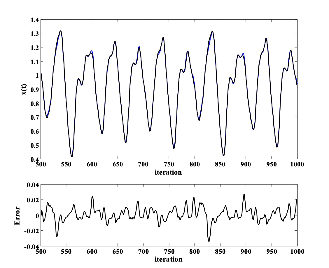
Figure 1: Top: Prediction output of ODE-DFS model (black line) and the testing points (blue line); Bottom: Residual prediction errors.

Table 1: Comparison Results of RMSE among various FPs.

Figure 2: Derivatives’ time-series $x^{\prime}(t),x^{\prime\prime}(t)$ and $x^{\prime\prime\prime}(t)$ (blue line – real series; black line – DFS series forecasting).

Table 1 reports the comparison of our fuzzy prediction method with other prediction methods, using the same data Crowder (1991). For this example, it can be seen that the performance of the presented method is superior to all the others listed on the table. Even so, our proposed method does not realise the optimisation of the partition of the input space. This methodology provides also the forecasting of the derivatives’ time-series. Fig. 2 represents the derivative time-series $x^{\prime}(t),x^{\prime\prime}(t)$ and $x^{\prime\prime\prime}(t),$ whose respective approximation MSE errors are $8.964\times 10^{-7},2.353\times 10^{-6}$ and $9.713\times 10^{-7}.$

6 Conclusions and future work

This paper presents a new methodology for prediction of complex discrete time systems or time-series. The approach is based on a DFS, combined with the ODE Taylor method. The DFS is a generalisation of the traditional FS that can incorporate relationships of the series in its linguistic fuzzy. In this way, DFS is capable of approximating regular functions, as well as the derivatives up to a given order, on compact domains. When the DFS model and its derivatives’ models are combined with the ODE Taylor method, the result is a capable algorithm to solve forecasting problems. This methodology was tested with the Mackey-Glass chaotic time-series forecasting problem. Comparative studies were carried out with other fuzzy and neural network predictors that suggest that our approach can offer comparable or even better performance. From our study, we conclude that efficiency in accurate and robust forecasting cannot rest solely on a good algorithm. For this reason, the method proposed in this work has the advantage of capturing and making explicit the derivatives of the time-series, which seems to us to be a quite desirable feature.

To continue the work, further comparison studies need to be done using other benchmark examples. Also, the performance of Taylor methods of higher order need to be investigated.

7 Acknowledgements

The authors would like to thank the reviewers for the valuable suggestions. Work financed by FCT - Fundação para a Ciência e a Tecnologia under project: (i) UIDB/04033/2020 for the first author. (ii) UIDB/00048/2020 for the second author.

References

• Cagcag Yolcu et al. (2016) Cagcag Yolcu, O., Yolcu, U., Egrioglu, E., and Aladag, C.H. (2016). High order fuzzy time series forecasting method based on an intersection operation. Applied Mathematical Modelling, 40(19), 8750–8765.
• Castillo and Melin (2020) Castillo, O. and Melin, P. (2020). Forecasting of covid-19 time series for countries in the world based on a hybrid approach combining the fractal dimension and fuzzy logic. Chaos, solitons, and fractals, 140.
• Christensen and Christensen (2004) Christensen, O. and Christensen, K. (2004). Approximation Theory, From Taylor Polynomials to Wavelests (Applied and Numerical Harmonic Analysis), 1st ed. Birkhäuser, Boston, MA.
• Crowder (1991) Crowder, R. (1991). Predicting the Mackey–Glass time series with cascade-correlation learning. In Proceedings of the 1990 Connectionist Models Summer School, NordiCHI, 117–123. Carnegie Mellon University, Pittsburgh, PA.
• Eyoh et al. (2017) Eyoh, I., John, R., and De Maere, G. (2017). Time series forecasting with interval type-2 intuitionistic fuzzy logic systems. In 2017 IEEE International Conference on Fuzzy Systems (FUZZ-IEEE), 1–6.
• Fan and Yao (2003) Fan, J. and Yao, Q. (2003). Nonlinear Time Series: Nonparametric and Parametric Methods. Springer, Berlin, Germany.
• Hamilton (1994) Hamilton, J.D. (1994). Time Series Analysis. Princeton University Press, Princeton, New Jersey.
• Jang et al. (1997) Jang, J.S.R., Sun, C.T., and E.Mizutani (1997). Neuro-Fuzzy and Soft Computing. Prentice- Hall, Englewood Cliffs, NJ.
• Kosko (1992) Kosko, B. (1992). Fuzzy system as universal approximators. In Proc. IEEE Int. Conf. Fuzzy Syst., 1153–1162. ACM, San Diego, CA.
• Maddala (1996) Maddala, G.S. (1996). Introduction to Econometrics. Prentice-Hall, Englewood Cliffs, NJ.
• Nguyen et al. (1996) Nguyen, H.T., Kreinovich, V., and Sirisaengtaksin, O. (1996). Fuzzy control as a universal control tooly. Fuzzy Sets Syst., 80, 71–86.
• Orang et al. (2022) Orang, O., de Lima e Silva, P.C., and Guimarães, F.G. (2022). Time series forecasting using fuzzy cognitive maps: A survey.
• Pedrycz and Gomide (1998) Pedrycz, W. and Gomide, F. (1998). An Introduction to Fuzzy Sets. MIT Press, Cambridge, MA.
• Pereira et al. (2015) Pereira, C.M., de Almeida, N.N., and Velloso, M.L. (2015). Fuzzy modeling to forecast an electric load time series. Procedia Computer Science, 55, 395–404.
• Pintelon and J.Schoukens (2006) Pintelon, R. and J.Schoukens (2006). Box–jenkins identification revisited—part i: Theory. Automatica, 42(1), 63–75.
• Refenes et al. (1997) Refenes, A.P.N., Burgess, A., and Y.Bentz (1997). Neural networks in financial engineering: a study in methodology. IEEE Transactions on Neural Networks, 8(6), 1222–1267.
• Rojas et al. (2008) Rojas, I., Valenzuela, O., Rojas, F., Guillen, A., L. J. Herrera, H.P., Marquez, L., and Pasadas, M. (2008). Soft-computing techniques and arma model for time series prediction. Neurocomputing, 71(4–6), 519–537.
• Salgado (2008) Salgado, P. (2008). Rule generation for hierarchical collaborative fuzzy system. Applied Mathematical Modelling, 32(7), 1159–1178.
• Sugeno and Yasukawa (1993) Sugeno, M. and Yasukawa, T. (1993). A fuzzy-logic-based approach to qualitative modeling. IEEE Transactions on Fuzzy Systems, 1(1), 7–.
• Takens (1980) Takens, F. (1980). Detecting strange attractors in turbulence. In D.A. Rand and L.S. Young (eds.), Dynamical Systems and Turbulences, Springer Lecture Notes in Mathematics, 365–381. Springer, New York, NY.
• Tsaur et al. (2005) Tsaur, R.C., O Yang, J.C., and Wang, H.F. (2005). Fuzzy relation analysis in fuzzy time series model. Computers and Mathematics with Applications, 49(4), 539–548.
• Tsoukalas and Uhrig (1997) Tsoukalas, L.H. and Uhrig, R.E. (1997). Fuzzy and Neural Approaches in Engineering. Wiley, New York, NY.
• Wan (1994) Wan, E.A. (1994). Time series prediction by using a connectionist network with internal delay lines. In A.S. Weigend and N.A. Gershenfeld (eds.), Time Series Prediction, Forecasting the Future and Understanding the Past, 175–195. Addison-Wesley, Reading, MA.
• Wang (1997) Wang, L.X. (1997). A course in fuzzy systems and control. Prentice-Hall, New Jersey, NJ.
• Wong and Tan (1994) Wong, F. and Tan, C. (1994). Hybrid neural, genetic, and fuzzy systems. In G.J. Deboeck (ed.), Neural, Genetic, and Fuzzy Systems for Chaotic Financial Markets, 243–262. Wiley, New York, NY.
• Yager and Filev (1994) Yager, R.R. and Filev, D. (1994). Essentials of Fuzzy Modeling and Control. Wiley, New York, NY.
• Yu and Zhang (2005) Yu, L. and Zhang, Y.Q. (2005). Evolutionary fuzzy neural networks for hybrid financial prediction. IEEE Transactions on Systems, Man, and Cybernetics, Part C (Applications and Reviews), 35(2), 244–249.
• Zeng and Singh (1995) Zeng, X.J. and Singh, M.G. (1995). Approximation theory of fuzzy systems-mimo case. IEEE Trans. Fuzzy Syst., 3, 219–235.
• Zhang et al. (1998) Zhang, G., Eddy Patuwo, B., and Y. Hu, M. (1998). Forecasting with artificial neural networks:: The state of the art. International Journal of Forecasting, 14(1), 35–62.
• Zhang et al. (2020) Zhang, Y., Qu, H., Wang, W., and Zhao, J. (2020). A novel fuzzy time series forecasting model based on multiple linear regression and time series clustering. Mathematical Problems in Engineering, 1, 1–18.