Guillotine Regularization: Why removing layers is needed to improve generalization in Self-Supervised Learning
Abstract
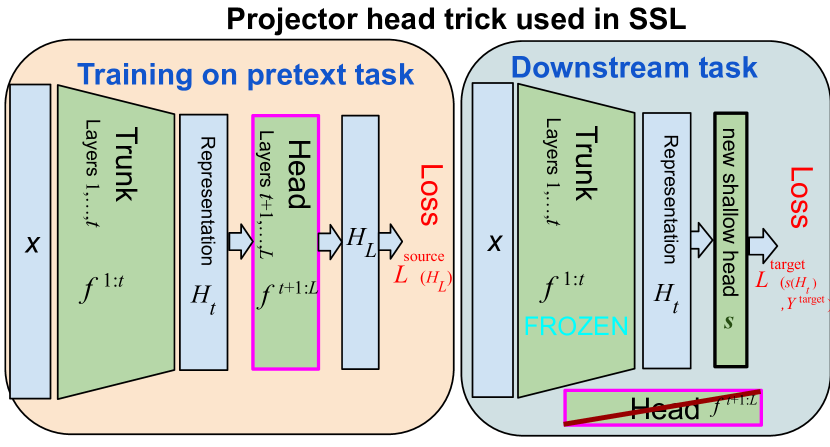
One unexpected technique that emerged in recent years consists in training a Deep Network (DN) with a Self-Supervised Learning (SSL) method, and using this network on downstream tasks but with its last few projector layers entirely removed. This trick of throwing away the projector is actually critical for SSL methods to display competitive performances on ImageNet for which more than percentage points can be gained that way. This is a little vexing, as one would hope that the network layer at which invariance is explicitly enforced by the SSL criterion during training (the last projector layer) should be the one to use for best generalization performance downstream. But it seems not to be, and this study sheds some light on why. This trick, which we name Guillotine Regularization (GR), is in fact a generically applicable method that has been used to improve generalization performance in transfer learning scenarios. In this work, we identify the underlying reasons behind its success and show that the optimal layer to use might change significantly depending on the training setup, the data or the downstream task. Lastly, we give some insights on how to reduce the need for a projector in SSL by aligning the pretext SSL task and the downstream task.
1 Introduction
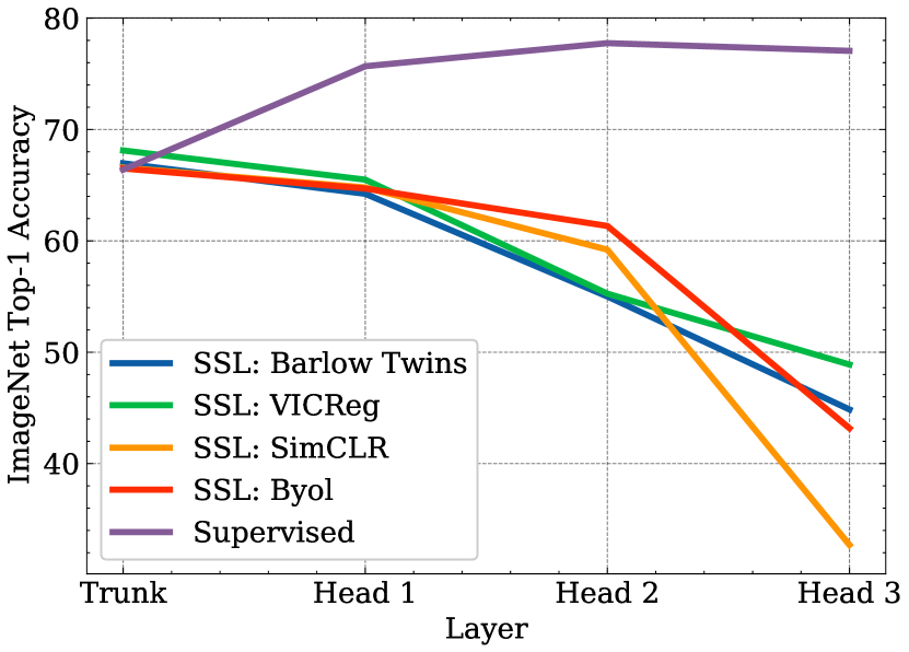
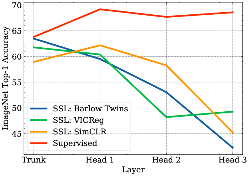
Many recent self-supervised learning (SSL) methods consist in learning invariances to specific chosen relations between samples – implemented through data-augmentations – while using a regularization strategy to avoid collapse of the representations (Chen et al., 2020a; c; Grill et al., 2020; Lee et al., 2021; Caron et al., 2020; Zbontar et al., 2021; Bardes et al., 2022; Tomasev et al., 2022; Caron et al., 2021; Chen et al., 2021; Li et al., 2022; Zhou et al., 2022a; b). Incidentally SSL learning frameworks also heavily rely on a simple trick to improve downstream task performances: removing the last few layers of the trained deep network depicted in Figure 1. From a practical viewpoint, this technique emerged naturally (Chen et al., 2020a) through the search of ever increasing SSL performances. In fact, on ImageNet (Deng et al., 2009), such technique can improve classification performances by around 30 points of percentage (Figure 1).
Although it improves performances in practice, not using the layer on which the SSL training was applied is unfortunate. It means throwing away the representation that was explicitly trained to be invariant to the chosen set of data augmentations, thus breaking the implied promise of using a more structured, controlled, invariant representation. By picking instead a representation that was produced an arbitrary number of layers above, SSL practitioners end up relying on a representation that likely contains much more information about the input (Bordes et al., 2021) than should be necessary to robustly solve downstream tasks.
Although the use of this technique emerged independently in SSL, using intermediate layers of a neural network–instead of the deepest layer where the initial training criterion was applied– has long been known to be useful in transfer learning scenarios (Yosinski et al., 2014). Features in upstream layers often appear more general and transferable to various downstream tasks than the ones at the deepest layers which are too specialized towards the initial training objective. This strongly suggests a related explanation for its success in SSL: does removing the last layers of a trained SSL model improve performances because of a misalignment between the SSL training task (source domain) and downstream task (target domain)?
In this paper, we examine that question thoroughly. We first place the SSL trick of removing the projector post-training under the umbrella of a generically applicable method that we call Guillotine Regularization. We argue that it is important to distinguish the action of removing layers during evaluation from architecture modifications because the optimal layer to use for a given downstream task is not always the backbone and could be intermediate projector’s layers. Then, we explore how changes in the training optimization, training data and downstream task impact the optimal layer in both supervised and self-supervised setting. Lastly, we demonstrate that increasing the *alignment* between the pretext and downstream task in SSL decreases the need to use a projector in SSL.

To summarize, this paper’s main contributions are the following:
-
•
Since the optimal layer to use in Self-Supervised-Learning might not always be the backbone, we suggest coining the action of removing layer as a general method called Guillotine Regularization to distinguish it from the architectural modification which is the addition of a projector.
-
•
To show through experiments that the optimal layer to cut heavily depend on the training optimization, training data and downstream task for both supervised and self-supervised models. We hope that this result will encourage the research community to run more systematic evaluations through different layers.
-
•
The need to use Guillotine Regularization in SSL depends heavily on how the positives views are defined. When these views are aligned with the downstream-task, the optimal layer to use become closer to the last layer.
2 Related work
Self-supervised learning
Many recent works on self-supervised learning (Chen et al., 2020a; c; Grill et al., 2020; Lee et al., 2021; Caron et al., 2020; Zbontar et al., 2021; Bardes et al., 2022; Tomasev et al., 2022; Caron et al., 2021; Chen et al., 2021; Li et al., 2022; Zhou et al., 2022a; b) rely on the addition of few non linear layers (MLP) – termed projection head – on top of a well established neural network – termed backbone – during training. This addition is done regardless of the neural network used as backbone, it could be a ResNet50 (He et al., 2016) or a Vision Transformer (Dosovitskiy et al., 2021). After training, the projector is usually threw away to evaluate the model using the backbone representation. Even if Chen et al. (2020b) demonstrated that the optimal layer to use might not always be the backbone when using few labelled data, most recent works introducing new SSL methods have continued to use only the backbone for evaluation. Some works also tried to understand why a projection head is needed for self-supervised learning. Appalaraju et al. (2020) argue that the nonlinear projection head acts as filter that can separate the information used for the downstream task from the information useful for the contrastive loss. In order to support this claim, they used deep image prior (Ulyanov et al., 2018) to perform features inversion to visualize the features at the backbone level and also at the projector level. They observe that features at the backbone level seem more suitable visually for a downstream classification task than the ones at the projector level. Another related work (Bordes et al., 2021) similarly tries to map back the representations to the input space, this time by using a conditional diffusion generative model. The authors present visual evidence confirming that much of the information about a given input is lost at the projector level while most of it is still present at the backbone level. Another line of work tries to train self-supervised models without the use of a projector. Jing et al. (2022) shows that by removing the projector and cutting the representation vector in two parts, such that a SSL criteria is applied on the first part of the vector while no criterion is applied on the second part, improves considerably the performances compared to applying the SSL criteria directly on the entire representation vector. This however works mostly thanks to the residual connection of the resnet. In contrast with these approaches, our work focus on identifying which components of traditional SSL training pipelines can explain why the performances when using the final layers of the network are so much worse than the ones at the backbone level. This identification will be key for designing future SSL setups in which the generalisation performance doesn’t drop drastically when using the embedding that the SSL criterion actually learns.
Transfer learning
The idea of using the intermediate layers of a neural network is very well known in the transfer learning community. Work like Deep Adaptation Network (Long et al., 2015) freeze the first layers of a neural network, fine-tune the last layers while adding a head which is specific for each target domain. The justification behind this strategy is that deep networks learn general features (Caruana, 1994; Bengio, 2012; Bengio et al., 2011), especially the ones at the first layers, that may be reused across different domain (Yosinski et al., 2014). Oquab et al. (2014) demonstrate that when limited amount of training data are available for the target tasks, using the frozen features extracted from the intermediate layers of a deep network trained on classification can help solve object and action classification tasks on other datasets. Another line of work on training with random or noisy labels also studied how the use of intermediate layers improves significantly downstream performances (Maennel et al., 2020) while Baldock et al. (2021) introduced a measure of example difficulty that leverages the number of intermediate layers that are aligned towards a given prediction. In this paper, we show that SSL trained models fall under the realm of transfer learning, in consequence we can expect that all the observations made in the transfer learning literature about the use of intermediate layers are also valid for SSL. When viewing the projector SSL trick and cutting layer for transfer as a general machine learning trick to improve generalization, it’s not surprising anymore that work as Wang et al. (2022); Sarıyıldız et al. (2023) have been able to show that adding a projector can also be highly beneficial for supervised training.
Out of distribution (OOD) generalization
Kirichenko et al. (2022) demonstrates that retraining only the last layer with a specific reweighting helps to "forget" the spurious correlations that were learned during the training. Such work emphasizes that most of the spurious correlation due to the training objective is contained in the last layers of the network. Thus, retraining them is essential to remove such spurious correlation and generalize better on downstream tasks. Similarly Rosenfeld et al. (2022) show that retraining only the last layers is most of the time as good as retraining the entire network over a subset of downstream tasks. Lastly, Evci et al. (2022) demonstrates the usefulness of using intermediate layers for OOD. Our study also confirms that Guillotine Regularization show important properties with respect to OOD generalization.
3 Guillotine Regularization: A regularization scheme to improve generalization of deep networks
In this section, we provide a definition for Guillotine Regularization. Then, through experiments, we show that the optimal layer to use changes significantly depending on different factors. Finally, we show that the performances at a given layer are not always correlated with the performances one can have at another layer.
3.1 (Re)Introducing Guillotine Regularization From First Principles
We distinguish between a source training task with its associated training set, and a target downstream task with its associated dataset111Terminology pretext-training / downstream comes from SSL, while source / target is used in transfer learning. It is the performance on the downstream task that is ultimately of interest. In the simplest of cases both tasks could be the same, with their datasets sampled i.i.d. from the same distribution. But more generally they may differ, as in SSL or transfer learning scenarios. In SSL we typically have an unsupervised training task, that uses a training set with no labels, while the downstream task can be a supervised classification task. Also note that while the bulk of training the model’s parameters happens with the training task, transferring to a different downstream task will require some additional, typically lighter, training, at least of a final layer specific for that task. In our study we will focus on the use of a representation computed by the network trained on the training task and then frozen, which gets fed to a simple linear layer that will be tuned for the downstream task. This "linear evaluation" procedure is typical in SSL and aims to evaluate the quality/usefulness of an unsupervised-trained representation. Our focus is to ensure good generalization to the downstream task. Note that training and downstream tasks may be misaligned in several different ways.
Informally, Guillotine Regularization consists in the following: for the downstream task, rather than using the last layer (layer ) representation from the network trained on the training task, instead use the representation from a few layers above (layer , with ). We thus remove a small multilayer "head" (layers to ) of the initially trained network, hence the name of the technique. We call the remaining part (layers 1 to ) the trunk222head / trunk are also known as projection head / backbone in the SSL literature.
Formally, we consider a deep network that takes an input and computes a sequence of intermediate representations through layer functions such that , starting from . The entire computation from input to last layer representation is thus a composition of layer functions333Precisely, a ”layer function” can correspond to a standard neural network layer (fully-connected, convolutional) with no residual or shortcut connections between them, or to entire blocks (as in densenet, or transformers) which may have internal shortcut connections, but none between them.:
The parameters and of trunk and head are then trained on the entire training set of examples of the training task (optionally with associated targets that we may have in transfer scenarios, but will typically be absent in SSL), to minimize the training task objective :
Then the multilayer head is discarded, we add to the trunk a (usually shallow) new head and we train its parameters , using the training set of examples for the downstream task , to minimize the downstream task objective :
3.2 An empirical analysis of situations in which cutting layers is beneficial
There are several situations that can create a misalignment between a training and a downstream task. Here we name of few:
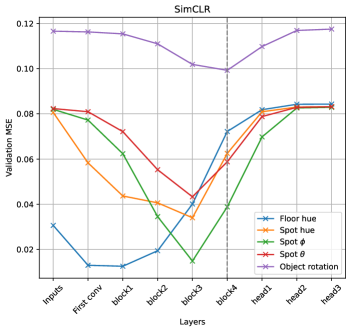
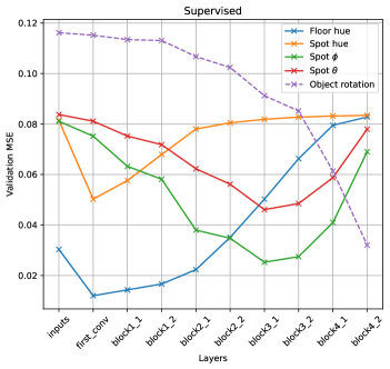
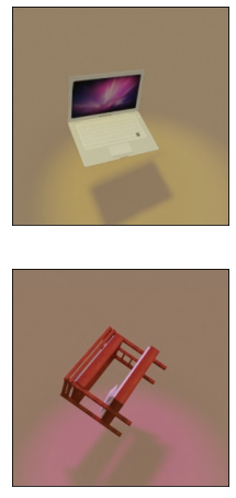
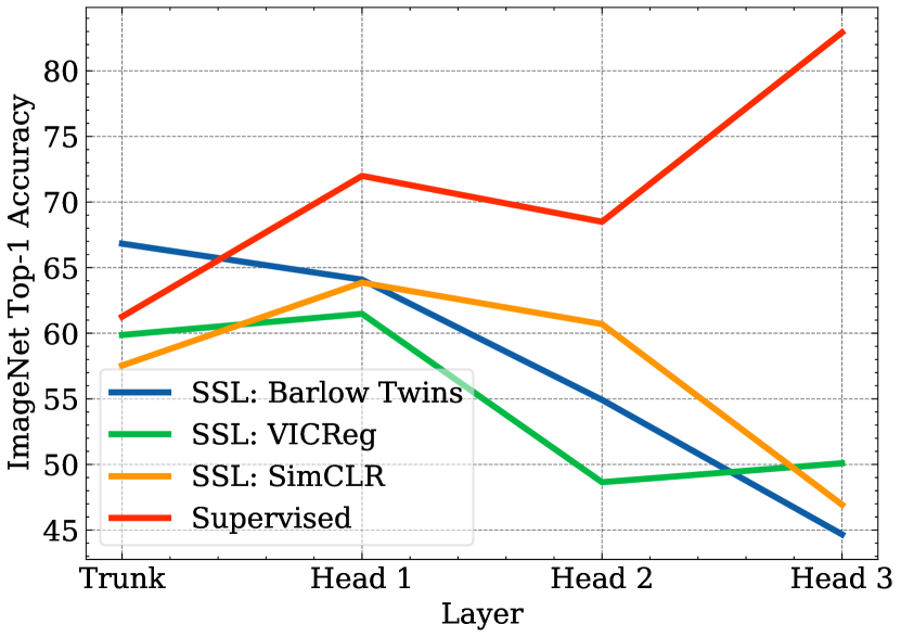
Misalignment between the training (source) and downstream (target) task while using the same input data distribution. The potential effectiveness of GR for transfer is not surprising since this technique has been used for years in the transfer learning research literature (Yosinski et al., 2014) to improve generalization across different tasks. As a simple illustration, we present Figure 2 which show how much performances on a given task can vary depending on which layer has been chosen as features extractor. In this figure, we used an artificially created object dataset in which we are able to play with different factors of variations. The dataset consists of renderings of 3D models from 3D warehouse (Trimble Inc, ). Each scene is built from a 3D object, a floor and a spot placed on top of the object to add lighting. This allows us to control every factor of variation and produce complex transformations in the scene. We vary the rotation of the object defined as a quaternion, the hue of the floor, and the spot hue as well as it position on a sphere using spherical coordinates. We provide more details on the dataset and rendering samples in the appendix. We observe in Figure 2 that when training a supervised model on the object rotation prediction task and evaluating the linear probe on the same task across different layers, the best results are obtained on the last layer. However, when using the same frozen neural network to predict other attributes like the Spot , the best performances are obtained few layers before the last one. Similarly, when training with a self-supervised objective (SimCLR), we can see that the different factors of variation are most easily retrievable before the projector. This means that representations before the projector will be more versatile as they will contain information that was removed by the pretraining task. For example if our downstream task is to predict the rotation, the representation at block4 will be optimal while if the downstream task is to predict the spot hue, the representation at the block 3 will be optimal. Such results highlight the need to use Guillotine Regularization when there is a shift in the prediction task. Moreover, the optimality of a layer depends on the downstream task.
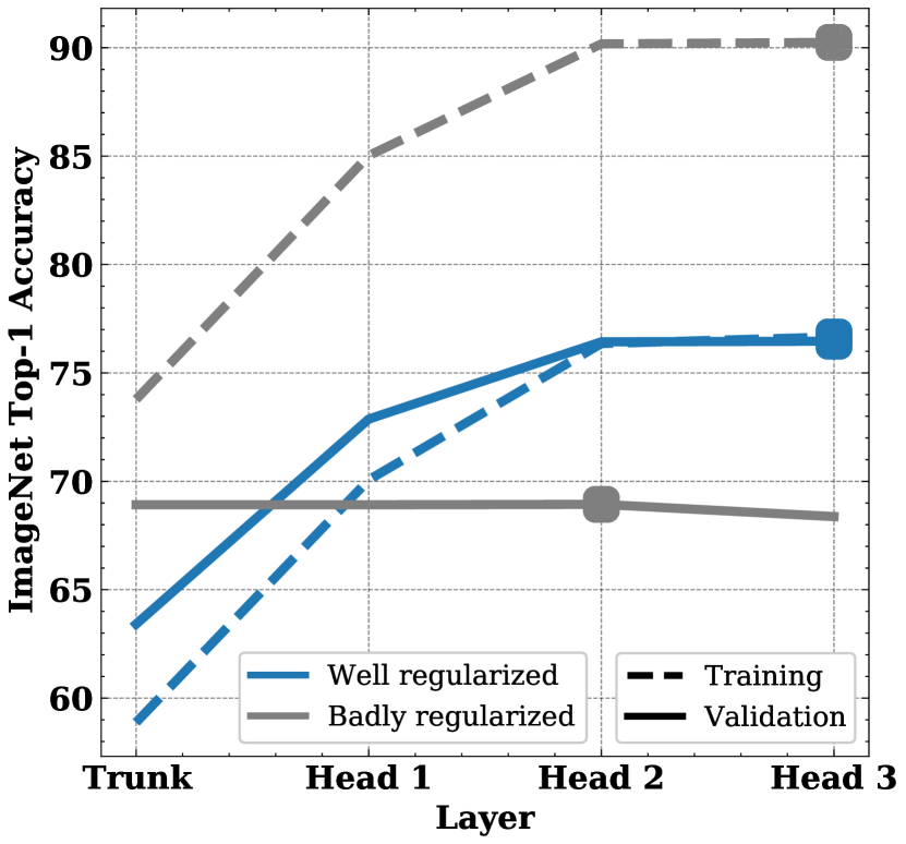
Misalignment due to badly optimized network It can be expected that the optimal layer to use to train a downstream task readout function might be different depending on how much the pretrained network is overfitting on the pretext task.
.
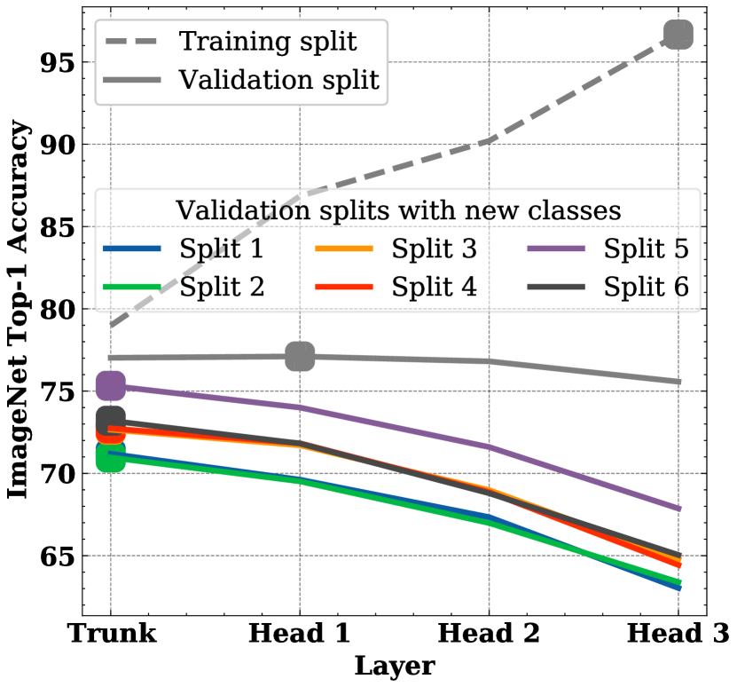
To test this hypothesis, we train a headed supervised Resnet50 on ImageNet with two different types of optimization. The first one using only AdamW with a small learning rate of without any additional regularization. The second one using SGD and the recommended hyper-parameters for a supervised training (with cycling learning rate, weight decay and momentum). In Figure 3(a), we observe that the AdamW trained network that is overfitting on the classification task has readout function performances that are very close across different layers. However, when looking at the well-regularized model with SGD which does not overfit on the task, the readout performances across layers vary significantly. In a second experiment, we study more in-depth the effect of overfitting by training the Resnet50 over only a random subset of 250 classes. Then we use the remaining 750 classes as an OOD validation set that is split randomly in other subset of 250 classes. In Figure 3(b), we clearly see that the training readout is overfitting on the training set while the readout performances across layers are similar on the corresponding in distribution validation set (which is similar to the previous experiment over the full ImageNet). Then, we train linear probes over the OOD splits and observe that the performances are radically different from the in distribution validation set. In fact, in this instance the best layer to use for every of these split is the backbone layer whereas the best layer to use for the in-distribution split is the projector layer. This result highlights that the optimal layer to discard can vary depending on the optimization techniques and downstream data distribution, even when the same training objective is used.
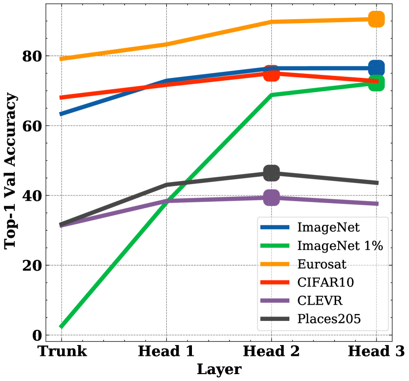
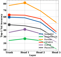
Misalignment between the training and downstream tasks while using different data distributions. When using a pretrained model to predict new classes, there is a bias in the data distribution as well as in the fine-tuning objective (with respect to the training settings). We did a first experiment in Figure 3(c) in which we train a supervised Resnet50 over ImageNet. Then, we freeze the weights of the model and train a linear probe over ImageNet (Deng et al., 2009), CIFAR10 (Krizhevsky, 2009), Place205 (Zhou et al., 2014), CLEVR (Johnson et al., 2017) and Eurosat (Helber et al., 2019) at different layers. We observe that the readout performances on ImageNet are the best at the last layer but for datasets like CLEVR or Place205 the best performances are obtained at the second projector layer. In Figure 4, we performed the same experiment but this time using SimCLR. In this instance, the best performances for ImageNet are obtained at the backbone whereas the best performances for Eurosat, CLEVR and Imagenet 1% are obtained at the first projector layer. This result challenges the common practice of discarding the entire projector in SSL since the layers to cut depend on the downstream task.
Misalignment between the training input data distribution and testing input data distribution while using the same training and downstream tasks. Another type of bias can arise when using a wrongful data distribution after training of the model.
| Head 3 | Head 2 | Head 1 | Trunk |
| 59.0 | 58.8 | 58.0 | 63.3 |
This scenario is often referred to Out Of Distribution (OOD) since the distribution of the data used by the model becomes different from the one seen during training. We took the supervised model trained on ImageNet along with the linear probe trained at different layers and evaluate the performances of these readouts on ImageNet-C (Hendrycks & Dietterich, 2019) which is a modified version of the validation set of ImageNet on which different data transformations were applied. Our experiment in Table 1 demonstrates that the performances are better after cutting two layers from the head of the network which highlight that it might be a good practice to probe intermediate representations when evaluating on OOD tasks.
3.3 The readout performances at the projector and backbone level are not always correlated
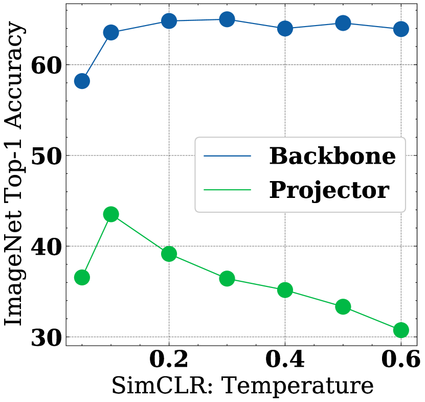


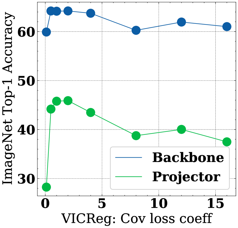
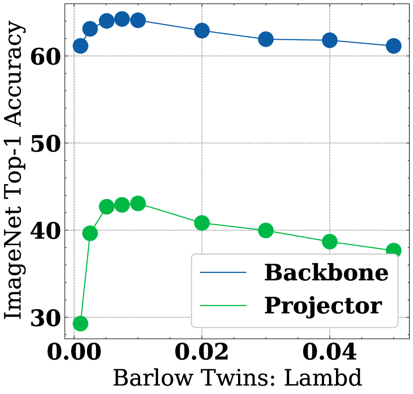
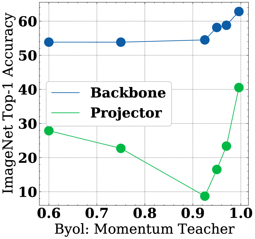
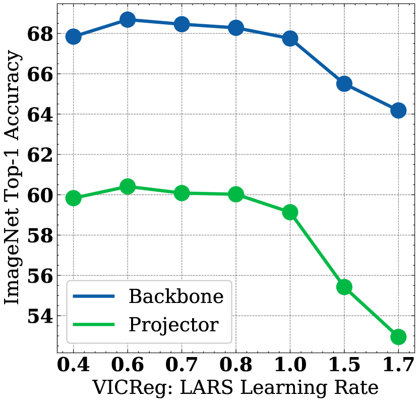
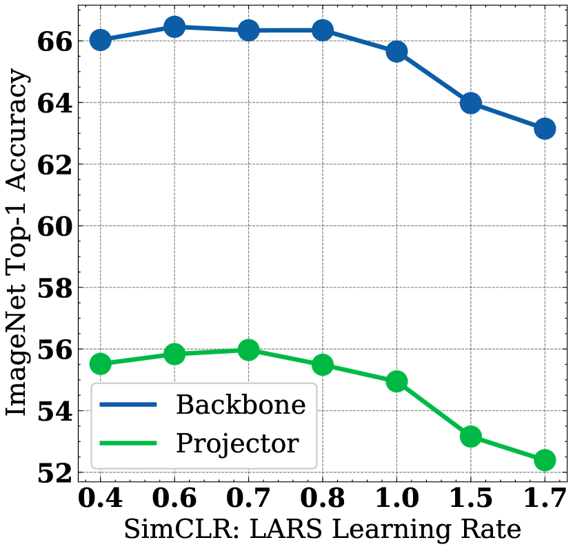
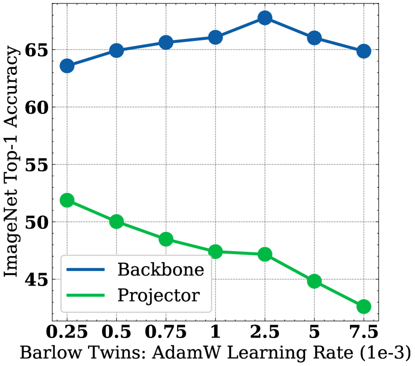
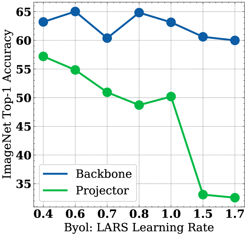
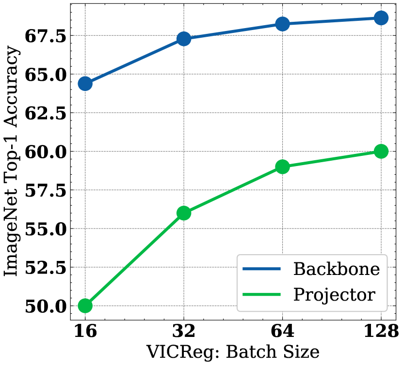
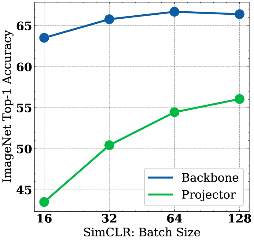
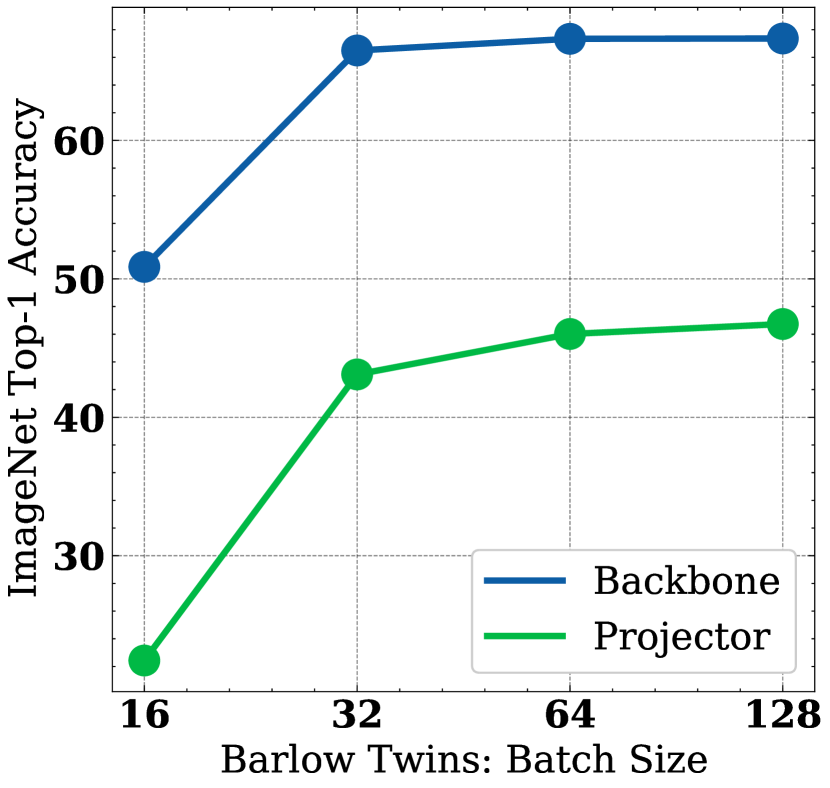
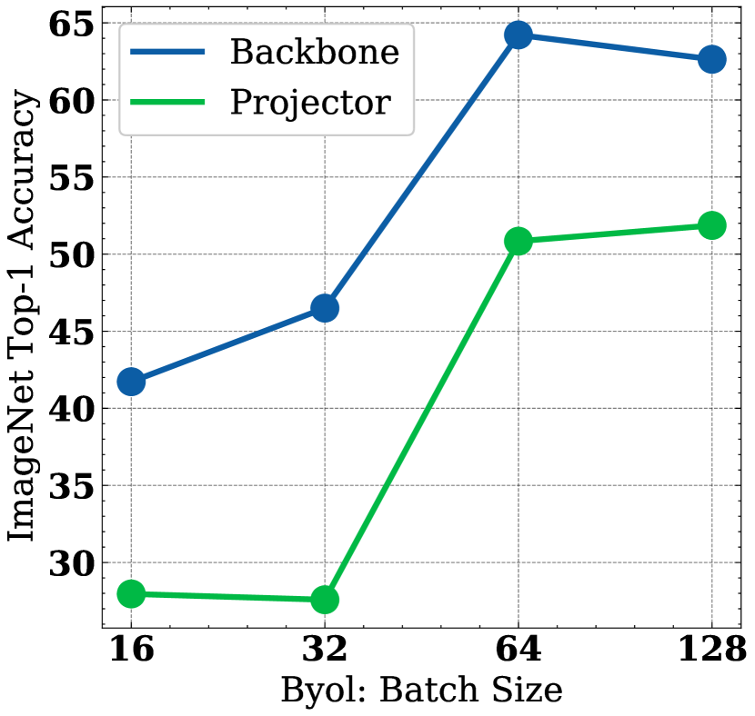
In Figure 5 we study the effect of Guillotine Regularization with respect to an hyper-parameter grid search for various SSL methods (SimCLR, Barlow Twins and Byol). When looking at the performances on ImageNet using a linear probe at the backbone level, one can observe an almost stable classification task performance for different hyper-parameters such as SimCLR temperature, Barlow Twins and Byol learning rate while the corresponding performances at the projector level change significantly. This highlights that the performances at the projector level are not always correlated with the performances at the backbone level. In consequence, knowing the performances of a linear probe at the projector level cannot give in advance insights about the performances at the backbone level.
4 Reducing the Need for a Projector in Self-Supervised Learning by increasing the alignment with the downstream task
Self-Supervised Learning is often considered a distinct learning paradigm in between supervised and unsupervised learning. In reality, the distinction is not as sharp, and much of SSL can be understood as solving a pretext-tasks akin to a supervised task(Wu et al., 2018; Khosla et al., 2020), merely with pseudo-labels obtained in another way than by human annotation. In this section, we show that different data selection process in SSL influences the alignment between the downstream and pretext task, which heavily impact the need of using a projector head in SSL.
To confirm the hypotheses that SSL methods need to use a projector because of a misalignement between the pretext and downstream task, we have to verify that reducing this misalignement, results in reducing the performance gap between the Trunk and Head representations. Ideally, we would like to get close to the supervised scenario in Figure 1 for which the optimal readout function is obtained at the last layer. To do so, we devise two experimental setups in which we replace the traditional data augmentation pipeline used in SSL, which consists of using handcrafted augmentation on each image to create a set of pairwise positive samples.
In the first setup, while using the exact same SSL criterion (SimCLR), we use as positive examples pairs of images that belong to the same class, and as negative examples images that don’t belong to the same class. Note that the SSL training criteria will push towards a collapse in the representation space of all the images belonging to the same class, while pushing further apart the different class clusters. By doing so the training SSL objective becomes perfectly aligned with the downstream classification task, despite using a SSL training criteria instead of a traditional cross entropy loss.
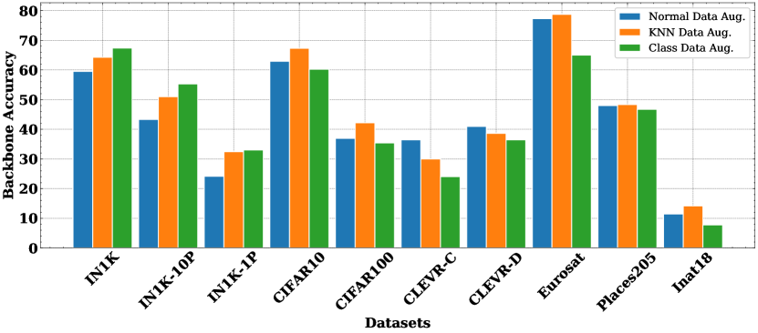
In the second setup, we use as positive pairs the closest neighbors found by a pretrained SSL model trained with the traditional SSL handcrafted data augmentation pipeline. The reasoning is that if instead of considering each image of the dataset as its own specific class, we use clusters of many images to define the positive pairs, we might be able to close the gap with respect to a supervised baseline without the need of labels.
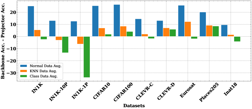
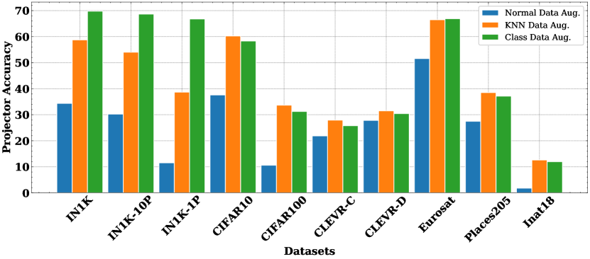
In Figure 6, we show the differences in accuracy between the backbone and the projector with respect to these two new data augmentation scenarios. The baseline, using the traditional SimCLR positive pairs based on data augmentations is in blue, the nearest neighbors setup in orange and the class based setup in green. We observe for SimCLR that using the nearest neighbors based heuristic is helping in reducing the gap between the pretext and downstream task while having a purely supervised heuristic to define the positive pair is removing the need to perform Guillotine Regularization across several downstream tasks. Hence confirming the hypothesis that the effectiveness of a projector depends of the alignment between the pretext and downstream task in self-supervised learning.
4.1 Visualizing the information across layers for different alignments
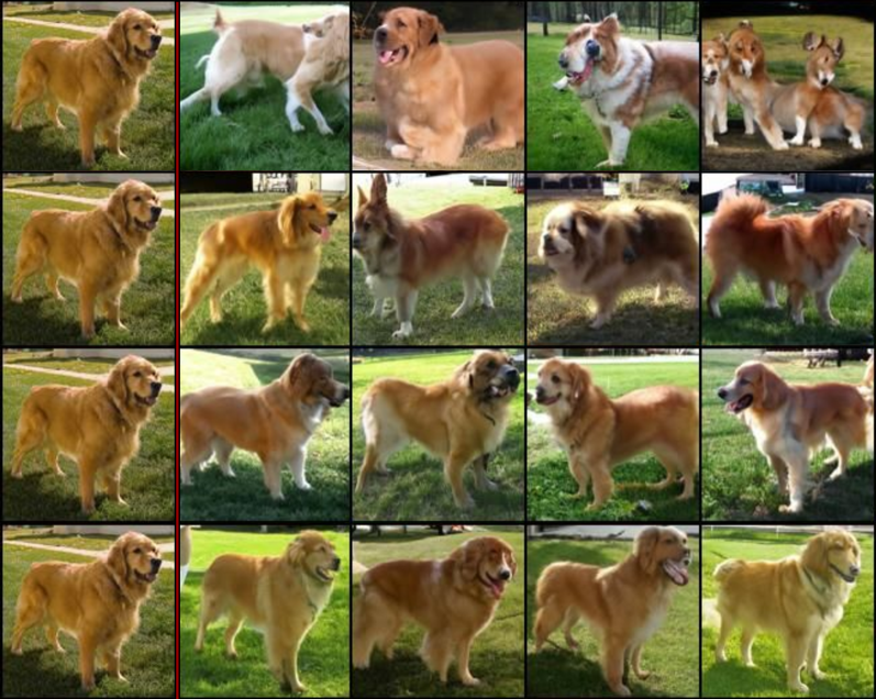
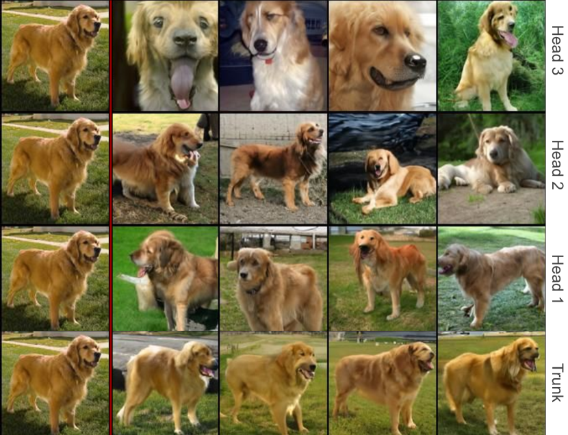
In this section, we use RCDM (Bordes et al., 2022), a conditional generative model to visualize what information is retain or not in the representation. We train RCDM on ImageNet with blurred faces(Yang et al., ), using the representation given by a SimCLR model trained on handcrafted SSL views and another which was trained on class based views. In Figure 7, we show that when looking at different decoding corresponding to different layers in the network, the information encoded vary a lot depending on the layer to use. When going deeper, RCDM is not able to reconstruct as much as information about the images than when using the backbone representation (which contain much more low level features). When looking at the generated samples that were conditioned on the representation of the model trained with supervised views, we observe that the breed of the dog stay the same across layers. However when using traditional data augmentations, the information about the specific golden retriever breed is lost in the last projector layers. This is correlated with the fact that this model get lower classification performances when using the projector.
4.2 Experimental details
We use Pytorch (Paszke et al., 2019) and FFCV-SSL (Bordes et al., 2023; Leclerc et al., 2022) as data loader. All the experiments were performed with a Resnet50 (He et al., 2016) (except if mentioned otherwise) as backbone. For each model, we use a batch of size 2048 and AdamW (Loshchilov & Hutter, 2019) as optimizer with an adaptive learning rate schedule. We run the training for 100 epochs. For each model, we add as head a small MLP of 3 layers of size 2048 (same dimension as the backbone) with ReLU (Glorot et al., 2011) as activation and batch normalization (Ioffe & Szegedy, 2015). When training different SSL methods, we always used the same set of data augmentations (with cropping, color-jitter, random grayscale, gaussian blur and solarization).
5 Conclusion
Through empirical evaluations, we demonstrated that the optimal layer to use for downstream evaluation vary depending on several factors: optimization, data and downstream task. These results highlight the need for SSL practitioners to run systematic evaluations at several layers instead of using always the backbone as reference. We also demonstrated that the use of a projector in SSL depends on the alignment between the downstream and pretext task. Despite, its usefulness, having to rely on a trick like Guillotine Regularization to increase performances reveals an important shortcoming of current self-supervised learning methods: the inability to design experimental setups and training criteria that learn structured and truly invariant representations with respect to an appropriate set of factors of variation. As future work, in order to escape from Guillotine Regularization, we should focus on finding new training criteria and data augmentations that will be more aligned with the downstream tasks of interest.
References
- Appalaraju et al. (2020) Srikar Appalaraju, Yi Zhu, Yusheng Xie, and István Fehérvári. Towards good practices in self-supervised representation learning. In NeurIPS Self-Supervision Workshop, 2020.
- Baldock et al. (2021) Robert J. N. Baldock, Hartmut Maennel, and Behnam Neyshabur. Deep learning through the lens of example difficulty. In Neural Information Processing Systems, 2021.
- Bardes et al. (2022) Adrien Bardes, Jean Ponce, and Yann LeCun. Vicreg: Variance-invariance-covariance regularization for self-supervised learning. In ICLR, 2022.
- Bengio (2012) Yoshua Bengio. Deep learning of representations for unsupervised and transfer learning. In Isabelle Guyon, Gideon Dror, Vincent Lemaire, Graham Taylor, and Daniel Silver (eds.), Proceedings of ICML Workshop on Unsupervised and Transfer Learning, volume 27 of Proceedings of Machine Learning Research, pp. 17–36, Bellevue, Washington, USA, 02 Jul 2012. PMLR. URL https://proceedings.mlr.press/v27/bengio12a.html.
- Bengio et al. (2011) Yoshua Bengio, Frédéric Bastien, Arnaud Bergeron, Nicolas Boulanger–Lewandowski, Thomas Breuel, Youssouf Chherawala, Moustapha Cisse, Myriam Côté, Dumitru Erhan, Jeremy Eustache, Xavier Glorot, Xavier Muller, Sylvain Pannetier Lebeuf, Razvan Pascanu, Salah Rifai, François Savard, and Guillaume Sicard. Deep learners benefit more from out-of-distribution examples. In Geoffrey Gordon, David Dunson, and Miroslav Dudík (eds.), Proceedings of the Fourteenth International Conference on Artificial Intelligence and Statistics, volume 15 of Proceedings of Machine Learning Research, pp. 164–172, Fort Lauderdale, FL, USA, 11–13 Apr 2011. PMLR. URL https://proceedings.mlr.press/v15/bengio11b.html.
- Bordes et al. (2021) Florian Bordes, Randall Balestriero, and Pascal Vincent. High fidelity visualization of what your self-supervised representation knows about. CoRR, abs/2112.09164, 2021. URL https://arxiv.org/abs/2112.09164.
- Bordes et al. (2022) Florian Bordes, Randall Balestriero, and Pascal Vincent. High fidelity visualization of what your self-supervised representation knows about. Transactions on Machine Learning Research, 2022. URL https://openreview.net/forum?id=urfWb7VjmL.
- Bordes et al. (2023) Florian Bordes, Randall Balestriero, and Pascal Vincent. Towards democratizing joint-embedding self-supervised learning, 2023. URL https://arxiv.org/abs/2303.01986.
- Caron et al. (2020) Mathilde Caron, Ishan Misra, Julien Mairal, Priya Goyal, Piotr Bojanowski, and Armand Joulin. Unsupervised learning of visual features by contrasting cluster assignments. In NeurIPS, 2020.
- Caron et al. (2021) Mathilde Caron, Hugo Touvron, Ishan Misra, Herve Jegou, and Julien Mairal Piotr Bojanowski Armand Joulin. Emerging properties in self-supervised vision transformers. In ICCV, 2021.
- Caruana (1994) Rich Caruana. Learning many related tasks at the same time with backpropagation. In G. Tesauro, D. Touretzky, and T. Leen (eds.), Advances in Neural Information Processing Systems, volume 7. MIT Press, 1994. URL https://proceedings.neurips.cc/paper/1994/file/0f840be9b8db4d3fbd5ba2ce59211f55-Paper.pdf.
- Chen et al. (2020a) Ting Chen, Simon Kornblith, Mohammad Norouzi, and Geoffrey E. Hinton. A simple framework for contrastive learning of visual representations. In ICML, 2020a.
- Chen et al. (2020b) Ting Chen, Simon Kornblith, Kevin Swersky, Mohammad Norouzi, and Geoffrey Hinton. Big self-supervised models are strong semi-supervised learners. In NeurIPS, 2020b.
- Chen et al. (2020c) Xinlei Chen, Haoqi Fan, Ross Girshick, and Kaiming He. Improved baselines with momentum contrastive learning. arXiv preprint arXiv:2003.04297, 2020c.
- Chen et al. (2021) Xinlei Chen, Saining Xie, and Kaiming He. An empirical study of training self-supervised vision transformers. In ICCV, 2021.
- Deng et al. (2009) Jia Deng, Wei Dong, Richard Socher, Li-Jia Li, Kai Li, and Li Fei-Fei. Imagenet: A large-scale hierarchical image database. In CVPR, 2009.
- Dosovitskiy et al. (2021) Alexey Dosovitskiy, Lucas Beyer, Alexander Kolesnikov, Dirk Weissenborn, Xiaohua Zhai, Thomas Unterthiner, Mostafa Dehghani, Matthias Minderer, Georg Heigold, Sylvain Gelly, Jakob Uszkoreit, and Neil Houlsby. An image is worth 16x16 words: Transformers for image recognition at scale. In ICLR, 2021.
- Evci et al. (2022) Utku Evci, Vincent Dumoulin, Hugo Larochelle, and Michael C Mozer. Head2Toe: Utilizing intermediate representations for better transfer learning. In Kamalika Chaudhuri, Stefanie Jegelka, Le Song, Csaba Szepesvari, Gang Niu, and Sivan Sabato (eds.), Proceedings of the 39th International Conference on Machine Learning, volume 162 of Proceedings of Machine Learning Research, pp. 6009–6033. PMLR, 17–23 Jul 2022. URL https://proceedings.mlr.press/v162/evci22a.html.
- Glorot et al. (2011) Xavier Glorot, Antoine Bordes, and Yoshua Bengio. Deep sparse rectifier neural networks. In Geoffrey Gordon, David Dunson, and Miroslav Dudík (eds.), Proceedings of the Fourteenth International Conference on Artificial Intelligence and Statistics, volume 15 of Proceedings of Machine Learning Research, pp. 315–323, Fort Lauderdale, FL, USA, 11–13 Apr 2011. PMLR. URL https://proceedings.mlr.press/v15/glorot11a.html.
- Grill et al. (2020) Jean-Bastien Grill, Florian Strub, Florent Altché, Corentin Tallec, Pierre H. Richemond, Elena Buchatskaya, Carl Doersch, Bernardo Avila Pires, Zhaohan Daniel Guo, Mohammad Gheshlaghi Azar, Bilal Piot, Koray Kavukcuoglu, Rémi Munos, and Michal Valko. Bootstrap your own latent: A new approach to self-supervised learning. In NeurIPS, 2020.
- He et al. (2016) Kaiming He, Xiangyu Zhang, Shaoqing Ren, and Jian Sun. Deep residual learning for image recognition. In CVPR, 2016.
- Helber et al. (2019) Patrick Helber, Benjamin Bischke, Andreas Dengel, and Damian Borth. Eurosat: A novel dataset and deep learning benchmark for land use and land cover classification. IEEE Journal of Selected Topics in Applied Earth Observations and Remote Sensing, 12(7):2217–2226, 2019. doi: 10.1109/JSTARS.2019.2918242.
- Hendrycks & Dietterich (2019) Dan Hendrycks and Thomas Dietterich. Benchmarking neural network robustness to common corruptions and perturbations. Proceedings of the International Conference on Learning Representations, 2019.
- Ioffe & Szegedy (2015) Sergey Ioffe and Christian Szegedy. Batch normalization: Accelerating deep network training by reducing internal covariate shift. In Francis Bach and David Blei (eds.), Proceedings of the 32nd International Conference on Machine Learning, volume 37 of Proceedings of Machine Learning Research, pp. 448–456, Lille, France, 07–09 Jul 2015. PMLR. URL https://proceedings.mlr.press/v37/ioffe15.html.
- Jing et al. (2022) Li Jing, Pascal Vincent, Yann LeCun, and Yuandong Tian. Understanding dimensional collapse in contrastive self-supervised learning. In ICLR, 2022.
- Johnson et al. (2017) Justin Johnson, Bharath Hariharan, Laurens van der Maaten, Li Fei-Fei, C Lawrence Zitnick, and Ross Girshick. Clevr: A diagnostic dataset for compositional language and elementary visual reasoning. In CVPR, 2017.
- Khosla et al. (2020) Prannay Khosla, Piotr Teterwak, Chen Wang, Aaron Sarna, Yonglong Tian, Phillip Isola, Aaron Maschinot, Ce Liu, and Dilip Krishnan. Supervised contrastive learning. In H. Larochelle, M. Ranzato, R. Hadsell, M.F. Balcan, and H. Lin (eds.), Advances in Neural Information Processing Systems, volume 33, pp. 18661–18673. Curran Associates, Inc., 2020. URL https://proceedings.neurips.cc/paper/2020/file/d89a66c7c80a29b1bdbab0f2a1a94af8-Paper.pdf.
- Kirichenko et al. (2022) Polina Kirichenko, Pavel Izmailov, and Andrew Gordon Wilson. Last layer re-training is sufficient for robustness to spurious correlations, 2022. URL https://arxiv.org/abs/2204.02937.
- Krizhevsky (2009) Alex Krizhevsky. Learning multiple layers of features from tiny images. pp. 32–33, 2009. URL https://www.cs.toronto.edu/~kriz/learning-features-2009-TR.pdf.
- Leclerc et al. (2022) Guillaume Leclerc, Andrew Ilyas, Logan Engstrom, Sung Min Park, Hadi Salman, and Aleksander Madry. ffcv. https://github.com/libffcv/ffcv/, 2022. commit xxxxxxx.
- Lee et al. (2021) Kuang-Huei Lee, Anurag Arnab, Sergio Guadarrama, John Canny, and Ian Fischer. Compressive visual representations. In NeurIPS, 2021.
- Li et al. (2022) Chunyuan Li, Jianwei Yang, Pengchuan Zhang, Mei Gao, Bin Xiao, Xiyang Dai, Lu Yuan, and Jianfeng Gao. Efficient self-supervised vision transformers for representation learning. In ICLR, 2022.
- Long et al. (2015) Mingsheng Long, Yue Cao, Jianmin Wang, and Michael I. Jordan. Learning transferable features with deep adaptation networks. In Proceedings of the 32nd International Conference on International Conference on Machine Learning - Volume 37, ICML’15, pp. 97–105. JMLR.org, 2015.
- Loshchilov & Hutter (2019) Ilya Loshchilov and Frank Hutter. Decoupled weight decay regularization. In 7th International Conference on Learning Representations, ICLR 2019, New Orleans, LA, USA, May 6-9, 2019. OpenReview.net, 2019. URL https://openreview.net/forum?id=Bkg6RiCqY7.
- Maennel et al. (2020) Hartmut Maennel, Ibrahim Alabdulmohsin, Ilya Tolstikhin, Robert J. N. Baldock, Olivier Bousquet, Sylvain Gelly, and Daniel Keysers. What do neural networks learn when trained with random labels? In Proceedings of the 34th International Conference on Neural Information Processing Systems, NIPS’20, Red Hook, NY, USA, 2020. Curran Associates Inc. ISBN 9781713829546.
- Oquab et al. (2014) Maxime Oquab, Leon Bottou, Ivan Laptev, and Josef Sivic. Learning and transferring mid-level image representations using convolutional neural networks. In Proceedings of the IEEE conference on computer vision and pattern recognition, pp. 1717–1724, 2014.
- Paszke et al. (2019) Adam Paszke, Sam Gross, Francisco Massa, Adam Lerer, James Bradbury, Gregory Chanan, Trevor Killeen, Zeming Lin, Natalia Gimelshein, Luca Antiga, Alban Desmaison, Andreas Kopf, Edward Yang, Zachary DeVito, Martin Raison, Alykhan Tejani, Sasank Chilamkurthy, Benoit Steiner, Lu Fang, Junjie Bai, and Soumith Chintala. Pytorch: An imperative style, high-performance deep learning library. In H. Wallach, H. Larochelle, A. Beygelzimer, F. d'Alché-Buc, E. Fox, and R. Garnett (eds.), Advances in Neural Information Processing Systems 32, pp. 8024–8035. Curran Associates, Inc., 2019. URL http://papers.neurips.cc/paper/9015-pytorch-an-imperative-style-high-performance-deep-learning-library.pdf.
- Rosenfeld et al. (2022) Elan Rosenfeld, Pradeep Ravikumar, and Andrej Risteski. Domain-adjusted regression or: Erm may already learn features sufficient for out-of-distribution generalization, 2022. URL https://arxiv.org/abs/2202.06856.
- Sarıyıldız et al. (2023) Mert Bülent Sarıyıldız, Yannis Kalantidis, Karteek Alahari, and Diane Larlus. No reason for no supervision: Improved generalization in supervised models. In The Eleventh International Conference on Learning Representations, 2023. URL https://openreview.net/forum?id=3Y5Uhf5KgGK.
- Tomasev et al. (2022) Nenad Tomasev, Ioana Bica, Brian McWilliams, Lars Buesing, Razvan Pascanu, Charles Blundell, and Jovana Mitrovic. Pushing the limits of self-supervised resnets: Can we outperform supervised learning without labels on imagenet? arXiv preprint arXiv:2201.05119, 2022.
- (41) Trimble Inc. 3d warehouse. https://3dwarehouse.sketchup.com/. Accessed: 2022-03-07.
- Ulyanov et al. (2018) Dmitry Ulyanov, Andrea Vedaldi, and Victor Lempitsky. Deep image prior. In CVPR, 2018.
- Wang et al. (2022) Yizhou Wang, Shixiang Tang, Feng Zhu, Lei Bai, Rui Zhao, Donglian Qi, and Wanli Ouyang. Revisiting the transferability of supervised pretraining: an MLP perspective. In IEEE/CVF Conference on Computer Vision and Pattern Recognition, CVPR 2022, New Orleans, LA, USA, June 18-24, 2022, pp. 9173–9183. IEEE, 2022. doi: 10.1109/CVPR52688.2022.00897. URL https://doi.org/10.1109/CVPR52688.2022.00897.
- Wu et al. (2018) Zhirong Wu, Yuanjun Xiong, X Yu Stella, and Dahua Lin. Unsupervised feature learning via non-parametric instance discrimination. In Proceedings of the IEEE Conference on Computer Vision and Pattern Recognition, 2018.
- (45) Kaiyu Yang, Jacqueline Yau, Li Fei-Fei, Jia Deng, and Olga Russakovsky. A study of face obfuscation in imagenet. In International Conference on Machine Learning (ICML).
- Yosinski et al. (2014) Jason Yosinski, Jeff Clune, Yoshua Bengio, and Hod Lipson. How transferable are features in deep neural networks? In Z. Ghahramani, M. Welling, C. Cortes, N. Lawrence, and K.Q. Weinberger (eds.), Advances in Neural Information Processing Systems, volume 27. Curran Associates, Inc., 2014. URL https://proceedings.neurips.cc/paper/2014/file/375c71349b295fbe2dcdca9206f20a06-Paper.pdf.
- Zbontar et al. (2021) Jure Zbontar, Li Jing, Ishan Misra, Yann LeCun, and Stéphane Deny. Barlow twins: Self-supervised learning via redundancy reduction. arXiv preprint arxiv:2103.03230, 2021.
- Zhou et al. (2014) Bolei Zhou, Agata Lapedriza, Jianxiong Xiao, Antonio Torralba, and Aude Oliva. Learning deep features for scene recognition using places database. In Z. Ghahramani, M. Welling, C. Cortes, N. Lawrence, and K.Q. Weinberger (eds.), Advances in Neural Information Processing Systems, volume 27. Curran Associates, Inc., 2014. URL https://proceedings.neurips.cc/paper/2014/file/3fe94a002317b5f9259f82690aeea4cd-Paper.pdf.
- Zhou et al. (2022a) Jinghao Zhou, Chen Wei, Huiyu Wang, Wei Shen, Cihang Xie, Alan Yuille, and Tao Kong. ibot: Image bert pre-training with online tokenizer. In ICLR, 2022a.
- Zhou et al. (2022b) Pan Zhou, Yichen Zhou, Chenyang Si, Weihao Yu, Teck Khim Ng, and Shuicheng Yan. Mugs: A multi-granular self-supervised learning framework. 2022b.
Appendix A Datasets
In this work, we use ImageNet (Deng et al., 2009) (Term of license on https://www.image-net.org/download.php) for our experiments. We also used a synthetic 3D dataset that will be described in the next subsection.
A.1 3D models dataset
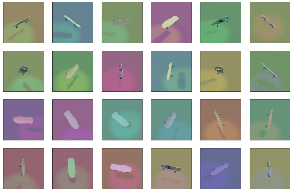
We will now discuss the dataset used for figure 2. As previously mentioned, this dataset consists of 3D models from 3D Warehouse (Trimble Inc, ), freely available under a General Model License, and rendered with Blender’s Python API. We alter the scene by uniformly varying the latent variables described in table 2.
| Latent variable | Min. value | Max. value |
|---|---|---|
| Object yaw | ||
| Object pitch | ||
| Object roll | ||
| Floor hue | ||
| Spot | ||
| Spot | ||
| Spot hue |
The variety in the scenes that can be generated is illustrated in figure 8. We can see that each latent variables can significantly impact the scene, giving a significant variety in the rendered images.
Appendix B Reproducibility
Our work does not introduce a novel algorithm nor a significant modification over already existing algorithm. Thus, to reproduce our results, one can simply use the public github repository of the following models: SimCLR, Barlow Twins, VicReg or the PyTorch Imagenet example (for supervised learning) with the following twist: adding a linear probe at each layer of the projector (and backbone) when evaluating the model. However, since many of these models can have different hyper-parameters, or data-augmentations, especially for the SSL models, we recommend to use a single code base with a given optimizer, a given set of data augmentations so that comparisons between models are fair and focus on the effect of Guillotine Regularization. In this paper, except if mentioned otherwise, we use as Head, a MLP with 3 layers of dimensions 2048 each (which match the number of dimensions at the trunk of a Resnet50) along with batch normalizaton and ReLU activations.
Appendix C Additional experimental results
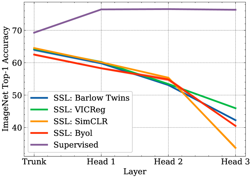
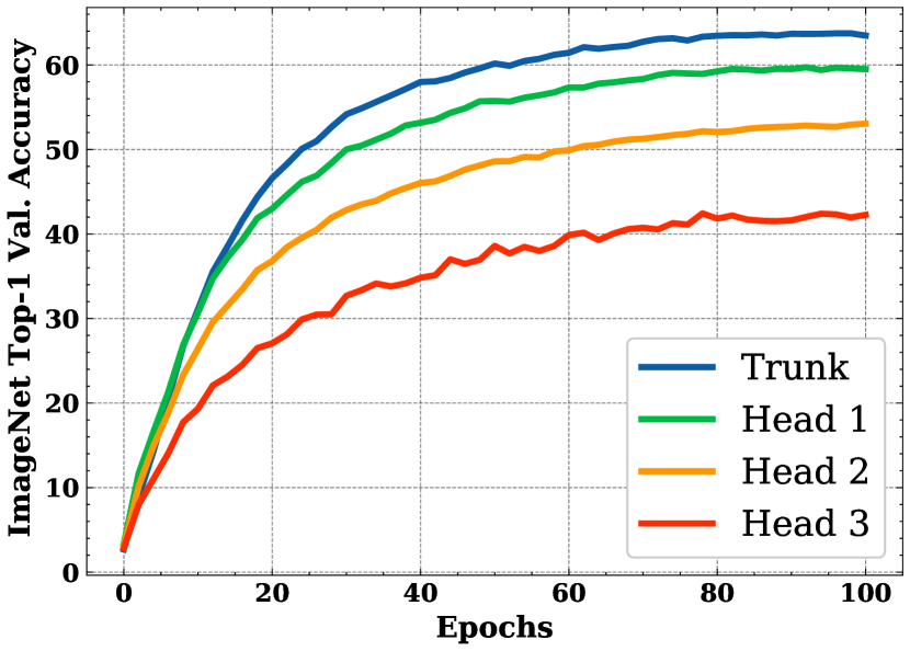
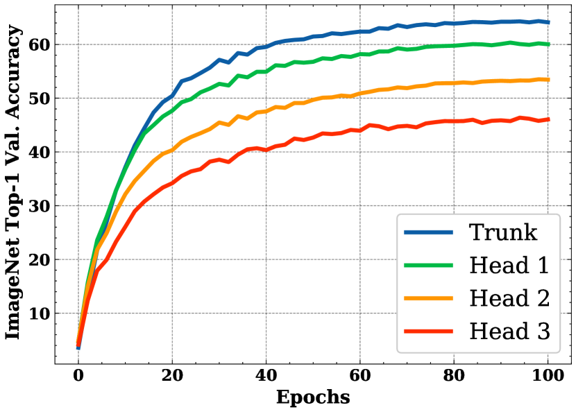
In this section, we present additional experimental results. The first one in Figure 9 is an extended version of Figure 1 with additional results on the training set. Figure 10 is a similar setup to the one in Figure 9 where we compared the performances at different layers for SSL methods and a supervised one except that we use a VIT-B instead of a Resnet50. We observe an important gap on the classification performances reached with a linear probe on different layers with the VIT-B when using SSL methods.
In Figure 11, we show how the performances at different layers change during training by using an online linear probing. At the beginning of the training the gap of performances between layers is low, however it increases significantly after 10 epochs.
In Figure 12 we show the accuracy computed with linear probes trained using projector and backbone representations. This figure is similar to Figure 6 except that we present the absolute accuracy value instead of the difference in accuracy with respect to the backbone.

Appendix D Limitations
In this work we focused mostly on analyzing the use of Guillotine Regularization in the context of Self-Supervised Learning. However, this kind of regularization might be useful for a variety of other types of training methods which we don’t investigate in this paper. We also mostly focus on generalization for classification tasks, but other tasks could also been worth exploring.