An Informational Approach to Exoplanet Characterization

Abstract

The atmospheres of exoplanets harbor critical information about their habitability. However, extracting and interpreting that information requires both high-quality spectroscopic data and a comparative analysis to characterize the findings. Looking forward to data availability, we propose a novel, assumption-free approach adapting the Jensen-Shannon divergence ($\mathcal{D}_{\rm{JS}}$) information measure to identify Earth-like planets through their transmission spectra. We apply this method to simulated Earth-like and Jupiter-like planets, including high-interest observed exoplanets such as Trappist-1e and GJ 667 Cc, and demonstrate that $\mathcal{D}_{\rm{JS}}$ can discriminate between different planet types. We argue that this method can be used to identify habitable and even inhabited planets as more precise transit spectroscopy data becomes available in the coming years.

1 Introduction

The search for other life in the universe is a question of central interest for science, with profound repercussions for culture and society. In recent decades, combined technological advances have allowed ground-based and space-borne missions like NASA’s Kepler space telescope (Lissauer et al., 2014) to rapidly expand the search for exoplanets, with over 5000 detections confirmed at the time of writing. With such a large pool of potential habitats to examine, the search for life has turned to planet characterization. Effective investigation of exoplanets with the potential to support life is thus of utmost importance. However, current investigations are limited by both the quality of observations of exoplanets and the unsettled debate of what planets qualify as “habitable” (Seager, 2014, 2013; Schwieterman et al., 2018). Upcoming missions such as the James Webb Space Telescope (JWST) (Gardner et al., 2006), Atmospheric Remote-sensing Infrared Exoplanet Large-survey (ARIEL) (Tinetti et al., 2018), Earth-2.0 (Ye et al., 2022), and the European Extremely Large Telescope (E-ELT) (Ramsay et al., 2020) promise to address the former problem, accelerating the need for a solution to the latter. This paper aims to address this concern.

Spectral analysis of exoplanetary atmospheres provides the most promising avenue for precise characterization of exoplanets. Direct detection of these atmospheres is difficult for smaller planets due to overwhelming glare from the host star (Birkby, 2018). However, transit spectropscopy provides an efficient method for characterizing terrestrial exoplanets. This method determines the spectrum of an exoplanet atmosphere by subtracting the host star spectrum from the spectrum of the star-planet system when the planet and its absorbing atmosphere are transiting the star. In 2002, Charbonneau et al. used transit spectroscopy to identify the presence of sodium in the atmosphere of HD 209458b, one of the pioneering works exploring exoplanet atmospheric composition (Charbonneau et al., 2002). Since then, exoplanet detections have led to a wealth of discoveries about the diversity of exoplanets (for examples see Diamond-Lowe et al. (2020), Kreidberg et al. (2014), Sing et al. (2016), and Benneke et al. (2019)), despite the narrow range of wavelengths covered by the Hubble Space Telescope (HST) and the Spitzer Telescope spectrographs. The available data provides insufficient information to fully characterize an exoplanet from its atmospheric spectrum. The upcoming telescope missions will capture a more complete high-resolution spectrum, increasing both the quality and quantity of spectral data.

Of particular interest are signs of life or habitability imprinted on these spectra. Lederberg (1965) and Lovelock (1965) first suggested that the presence of life would allow a planetary atmosphere to sustain out-of-equilibrium conditions. Some of these so-called biosignatures will be detectable with upcoming telescope missions (Thompson et al., 2022; Tinetti et al., 2021; Udry et al., 2014). Signs of planet habitability - such as the presence of water or carbon chemistry - would be visible in the atmospheric spectrum (Schwieterman et al., 2018). However, open questions concerning biosignatures present challenges to discriminate between exoplanets and the details of their atmospheric spectra. Among them, we list the habitability of the inner radius of the habitable zone, whether life is viable with a liquid solvent other than water or a molecular base other than carbon, the possibility of life in subsurface oceans, and the differences between life-driven or geophysical-driven out-of-equilibrium atmospheric chemistry (Schwieterman et al., 2018; Seager, 2014; Kaltenegger, 2017). Given these and other unknowns, we will assume here that the biosignatures we can currently analyse with confidence are those that closely mimic what we expect from ”life as we know it.” One of the strengths of our information-theory approach is its flexibility to be adapted as our understanding of life elsewhere evolves.

In this paper, we propose an information-theory based method designed to be be applied to transit spectroscopy. The method is designed to identify Earth-like planets in a conjecture-free manner. By quantifying the information content contained in the exoplanetary spectrum, we are able to identify spectra similar to that of Earth’s. We illustrate this method by comparing simulated exoplanets to a simulated Earth spectrum. We show that our information measure efficiently differentiates between Earth-like and Jupiter-like planets. We also demonstrate that how our method is sensitive to variations in physical parameters. Section 2 describes the information theory metric we employ to differentiate planets. Section 3 describes the simulations used to obtain data for this analysis. Section 4 shows how our method is affected by varying the physical parameters for a sample Jupiter-like planet. This demonstrates the ability of our method to differentiate between planet types and to identify changes in planetary features. Section 5 shows results for a series of simulations of real hot Jupiter and super-Earth exoplanets. We compare these exoplanets with simulated spectra of Earth, Jupiter, and a hot Jupiter clone to show how our method is able to discriminate between types of planets with realistic, diverse variations in planetary features. Section 6 summarizes our results and expands on how the method may be used to identify biosignatures associated with inhabited planets.

2 Information Measure

We quantify the dissimilarity between two planetary spectra as the difference between the information contents contained in the two spectra. We begin transforming the spectra into modal fractions, probability distributions introduced by Gleiser & Stamatopoulos (2012a) that give the relative weight of each wave mode. Since transit spectra are discrete and already in Fourier space, the modal fraction $p_{\nu}$ at a particular wave number, $\nu$, is simply

$$p_{\nu}=\frac{D_{\nu}}{\sum_{\nu}D_{\nu}},$$ (1)

for $D_{\nu}$ the transit depth of the spectrum at a particular wave number. The information content of each spectrum can then be quantified through its Shannon entropy, $H$, given by

$$H=\sum_{\nu}p_{\nu}log(p_{\nu}),$$ (2)

for $p_{\nu}$ the modal fraction at wave number $\nu$ (Shannon, 1948). The information required to discriminate between two modal fractions $p$ and $q$ is then given by the Kullback-Leibler Divergence (Kullback & Leibler, 1951),

$$\mathcal{D}_{KL}(p||q)=\sum_{\nu}p_{\nu}log(\frac{p_{\nu}}{q_{\nu}}).$$ (3)

However, this information measure is not symmetric about exchange of spectra - the information loss measured by $\mathcal{D}_{\rm{KL}}(p||q)$ is not the same as that measured by $\mathcal{D}_{\rm{KL}}(q||p)$. To ameliorate this, a symmetrized information criteria, Jensen-Shannon Divergence, was developed by Lin (1991). This creates a true measure of the divergence in information content between two modal fractions. The Jensen-Shannon Divergence, $\mathcal{D}_{\rm{JS}}(p||q)$, of two probability distributions is given by

$$\mathcal{D}_{JS}(p||q)=\frac{1}{2}\mathcal{D}_{\rm{KL}}(p||r)+\frac{1}{2}\mathcal{D}_{\rm{KL}}(q||r),$$ (4)

where $r=\frac{1}{2}(p+q)$.

In contrast to previous methods of exoplanet characterization, $\mathcal{D}_{\rm{JS}}$ requires no prior knowledge to interpret the spectrum. This is critical - biosignatures or signs of habitability may resemble Earth’s atmosphere in ways we cannot predict a priori. Relying on our incomplete understanding of the diversity of scenarios that may host life could cause us to miss inhabited planets.

We note that $\mathcal{D}_{\rm{JS}}$ alone is not able to isolate biosignatures as it measures the difference in information content of the full spectrum rather than individual absorption lines. (We can think of it as a global quantity obtained from a given spectrum, like the area of a function obtained from its integral.) Identification of biosignatures requires some form of input knowledge (e.g., specific compounds related to biotic activity), while $\mathcal{D}_{\rm{JS}}$ requires none. In an accompanying paper we will show how the $\mathcal{D}_{\rm{JS}}$-density per wave number can be used to isolate specifc biosignatures in planetary spectra with limited input knowledge (cf. Eq. 14 in (Gleiser & Stamatopoulos, 2012b)). Together, these two uses of $\mathcal{D}_{\rm{JS}}$ allow for both the identification of a planetary type (this paper) and for a detailed characterization of an exoplanet’s atmospheric composition. The global $\mathcal{D}_{\rm{JS}}$ may be used to search for exoplanets with the potential to host life, while the $\mathcal{D}_{\rm{JS}}$ density may identify which of those exoplanets may actually be inhabited.

3 Data

We demonstrate that $\mathcal{D}_{\rm{JS}}$ can be used to differentiate different types of exoplanets using simulations from the radiative transfer code Exo-Transmit (Kempton et al., 2017). The simulations are governed by seven parameters - equilibrium temperature used for a temperature-pressure profile, atmospheric equation of state, planetary surface gravity, planetary radius, stellar radius, and two parameters controlling the effect of haze in the atmosphere - cloud top pressure and a parameter controlling the strength of Rayleigh scattering. For all of our simulations, we chose to set a fixed value for the Rayleigh scattering parameter while allowing the code to calculate the cloud top pressure. We used literature values of each of the parameters to simulate an Earth spectrum and a Jupiter spectrum. We created a series of Jupiter clones with each individual parameter varied in isolation to demonstrate their effects on $\mathcal{D}_{\rm{JS}}$, shown in Section 4. We also simulated realistic hot Jupiters and super-Earths to demonstrate the ability of $\mathcal{D}_{\rm{JS}}$ to differentiate between planet types. For each exoplanet class, we create ten planet simulations - six from observed exoplanets using parameter values from literature, and four artificial planets designed to explore the parameter space. The parameters used to create these exoplanets are shown in Table 3. For comparison with the exoplanets, we simulate a Jupiter spectrum, an Earth spectrum, and the spectrum of a Jupiter clone with the temperature raised to 1200K. These results are shown in Section 5.

Table 1: The parameters used to generate realistic exoplanet simulations. The hot Jupiter simulations are shown in the top half of the table while the super-Earths are shown in the bottom half. The two planetary classes are separated by a horizontal line.

Name	Equilibrium Temperature
	Equation of State
	Surface Gravity
	Planet Radius
	Stellar Radius
	Rayleigh Scattering
	(Augmentation factor)
Jupitera	300	1X	24.79	6.99$\times$107	6.96$\times$108	10
HAT-P-1bb	1300	5X with graphite rainout	7.5	9.44$\times$107	8.17$\times$108	10
HAT-P-12bc	1000	1X	5.6	6.86$\times$107	4.87$\times$108	200
HD 189733bd	1200	1X	21.4	8.15$\times$107	5.60$\times$108	500
HD 209458be	1500	0.1X	9.4	9.72$\times$107	8.35$\times$108	10
WASP-6bf	1200	1X	8.7	8.72$\times$107	6.05$\times$108	1000
WASP-39bg	1100	1X	4.1	9.08$\times$107	6.23$\times$108	1
Hot Jupiter simulation 1	1400	5X with graphite rainout	12.8	8.45$\times$107	5.02$\times$108	1000
Hot Jupiter simulation 2	700	1X	20.1	6.27$\times$107	8.95$\times$108	100
Hot Jupiter simulation 3	1000	1X, 0.2 C-to-O ratio	8.8	9.23$\times$107	6.48$\times$108	10
Hot Jupiter simulation 4	1300	1X , 0.8 C-to-0 ratio	17.2	6.90$\times$107	9.23$\times$108	1
Earthh	300	1X	9.8	6.37$\times$106	6.96$\times$108	1
Proxima bi	300	1X	10.9	6.82$\times$106	9.82$\times$107	1
Trappist-1ej	300	1X	7.2	5.85$\times$106	8.15$\times$107	1
GJ 15 Abk	300	0.1X	12.4	9.88$\times$106	2.85$\times$108	10
GJ 667 Ccl	300	0.1X	15.7	9.81$\times$106	2.92$\times$108	1
CD Cet bm	500	1X	11.7	1.16$\times$107	1.18$\times$108	0
EPIC 24983012bn	1500	1X	22.6	1.24$\times$107	1.19$\times$109	1
Simulated super-Earth 1	700	1X	14.8	9.87$\times$106	8.80$\times$108	10
Simulated super-Earth 2	400	5X	10.4	6.02$\times$106	4.53$\times$108	1
Simulated super-Earth 3	300	1X	8.4	7.12$\times$106	9.25$\times$108	1000
Simulated super-Earth 4	1000	10X	12.8	8.54$\times$106	1.02$\times$109	1

Note. — ^a Sources: Montañes-Rodriguez et al. (2015); Sato & Hansen (1979)  ^bSource: Liu et al. (2014)  ^cSource: Hartman et al. (2009)  ^dSource :Boyajian et al. (2015)  ^eSource: del Burgo & Allende Prieto (2016)  ^fSource: Gillon et al. (2009)  ^gSource: Faedi et al. (2011)  ^hSource: Kempton et al. (2017)  ⁱ Sources:Lin & Kaltenegger (2020); Barnes et al. (2016)  ^jSources: Lin & Kaltenegger (2020); Delrez et al. (2018)  ^kSource: Pinamonti et al. (2018)  ^lSource: Anglada-Escudé et al. (2013) ^mSource: Bauer et al. (2020)  ⁿSource: Hidalgo et al. (2020)

4 Results 1: Spectra from Changing Physical Parameters

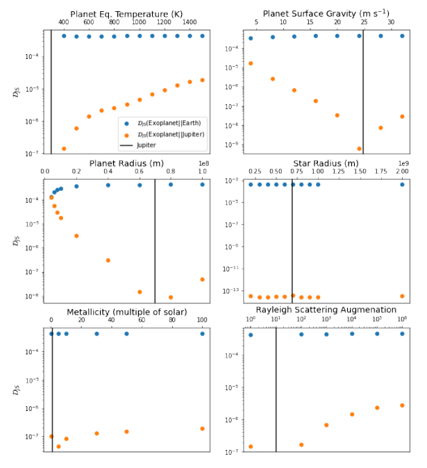
Figure 1: $\mathcal{D}_{\rm{JS}}$ of a simulated, Jupiter-like exoplanet compared to Earth (blue dots) and to Jupiter (orange dots). Each plot represents the variation of one parameter. The vertical black line indicates the Jupiter value of the parameter.

Fig. 1 shows how varying the input parameters in isolation affects the $\mathcal{D}_{\rm{JS}}$ relative to Earth and Jupiter. This figure illustrates two main results. The first is that $\mathcal{D}_{\rm{JS}}$ is sensitive to variations in planetary features. Variations in the planetary parameters away from their Jupiter values (vertical black line) incrementally increase the $\mathcal{D}_{\rm{JS}}$ relative to Jupiter, displaying the growing dissimilarity between the two planets.

Each of the plots tells a story illustrating the ability of $\mathcal{D}_{\rm{JS}}$ to pick up on underlying physics. Using the modal fraction ensures that the information content is not dependent on the continuum flux, only on the relative strength and shape of the absorption lines. For equilibrium temperature, surface gravity, planet radius, stellar radius - the top two rows of plots - varying the parameters varies the strength of the absorption lines in the modal fraction. For example, the scale height, $H$, of the planetary atmosphere is linearly dependent on the temperature, $T$, given by

$$H=\frac{k_{B}}{\mu_{m}g}T,$$ (5)

for $k_{B}$ the Boltzmann constant, $\mu_{m}$ the mean molecular mass, and $g$ the surface gravity on the planet. Increasing the scale height increases the size of the light-absorbing atmosphere. Therefore, the absorption line strength grows with temperature. As the strength of the exoplanet absorption lines diverges from the strength of the absorption lines in the Jupiter spectrum, the information contained in the two spectra also diverge. Vice versa, decreasing the temperature decreases the strength of the absorption lines. This results in a valley in the temperature plot (top left) where the lowest point in $\mathcal{D}_{\rm{JS}}$ - highest similarity between the two planets - sits nearest the Jupiter temperature (black line), while increasing incrementally as the temperature increases. Since, except for metallicity and Rayleigh scattering, changing the parameters away from the Jupiter value impacts the strength of the absorption lines, we see a valley occurring in nearly all plots. This illustrates the reliability of our approach to distinguish between different planetary types. We note that the stellar radius plot in the middle right indicates that small variations in the stellar radius make little impact compared to variations in the other parameters. This is represented by extremely low (of order $10^{-13}$) values of $\mathcal{D}_{\rm{JS}}$ relative to Jupiter for the range of parameter values we analysed.

Increasing the strength of Rayleigh scattering causes information divergence not by impacting the strength of the absorption lines, but by creating a spectral tilt in the near-IR (Des Etangs et al., 2008). This reduces $\mathcal{D}_{\rm{JS}}$ at the low wavelength absorption lines in the spectrum. Therefore, just as with the other parameters, the values of the Rayleigh scattering factor closest to Jupiter’s have the lowest $\mathcal{D}_{\rm{JS}}$. Similarly, changing the metallicity impacts the relative strength of absorption lines for different molecules. As a consequence, metallicities closest to Jupiter have the lowest $\mathcal{D}_{\rm{JS}}$, although the differences are relatively small (smaller than an order of magnitude) compared to other physical parameters.

The second key result from the parameter variation analysis is that the values of $\mathcal{D}_{\rm{JS}}$ comparing the modified Jupiters to Earth (blue dots) are consistently higher than those comparing to Jupiter. This indicates that our method is able to distinguish Earth-like and Jupiter-like planets for a wide range of parameters. The only exception occurs at the smallest planet radius in the middle left plot. As the planetary radius is decreased to even smaller values than the Earth radius, the $\mathcal{D}_{\rm{JS}}$ compared to Jupiter and to Earth approach each other. This does not indicate that the planet is similar to Earth. Rather, it indicates that the distance in information space between the planet and Jupiter is similar to the distance between the planet and Earth, albeit in different directions. For the planet and Earth to be similar, the $\mathcal{D}_{\rm{JS}}$ between the two would need to be small.

5 Results 2: Differentiating exoplanet types

In the previous section, we investigated the effects of changing a single physical parameter at a time to test the reliability of $\mathcal{D}_{\rm{JS}}$ as a discriminator of types of exoplanets under different conditions. Of course, the universe does not allow one physical parameter to be changed in isolation. Rather, the physical parameters controlling an exoplanet spectrum are often interdependent. Moving thus toward more concrete situations, in this Section we simulate a collection of observed super-Earths and hot Jupiters to show that $\mathcal{D}_{\rm{JS}}$ can indeed differentiate between the planet classes. We compare the two classes of planets to simulated Earth and Jupiter spectra, as well as to the spectrum of a Jupiter clone with the equilibrium temperature increased to 1200K. Our results show that $\mathcal{D}_{\rm{JS}}$ can identify which of the simulated worlds is closest to Jupiter or to Earth.

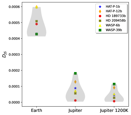
Figure 2: Violin plot showing the $\mathcal{D}_{\rm{JS}}$ distributions comparing the simulated hot Jupiters to Earth (left), to Jupiter (center), and to a Jupiter-clone with the temperature raised to 1200K (right). The width of the violin plot reads like a histogram, indicating the distribution of planets clustered around the mean $\mathcal{D}_{\rm{JS}}$ value. The $\mathcal{D}_{\rm{JS}}$ from six observed exoplanets are labeled with colored shapes; remaining points in the $\mathcal{D}_{\rm{JS}}$ distribution are from four exoplanet simulations. Physical parameters for the exoplanets are listed in Table 3.

In Fig. 2, we find that the $\mathcal{D}_{\rm{JS}}$ distribution comparing the six hot Jupiters to the two Jupiter-like planets do not overlap with the $\mathcal{D}_{\rm{JS}}$ distribution comparing them to Earth. This illustrates that $\mathcal{D}_{\rm{JS}}$ is able to distinguish between Jupiter-like and Earth-like planets. There is, however, an overlap between the two distributions comparing the hot Jupiters to Jupiter and to 1200K Jupiter. This is due to the similarity of the comparison planets. Still, the mean (bulge in the gray violin plots) of the 1200K Jupiter $\mathcal{D}_{\rm{JS}}$ distribution is the lower of the two distributions, indicating that $\mathcal{D}_{\rm{JS}}$ is able to identify the temperature similarity of the hot Jupiters and the hotter, 1200K Jupiter clone. We also show the results of specific comparisons for the six hot Jupiters, each labeled by a different colored shape. For example, planet WASP-39b (identified by a green square) is clearly a hot Jupiter, most similar to the simulated Jupiter at 1200K.

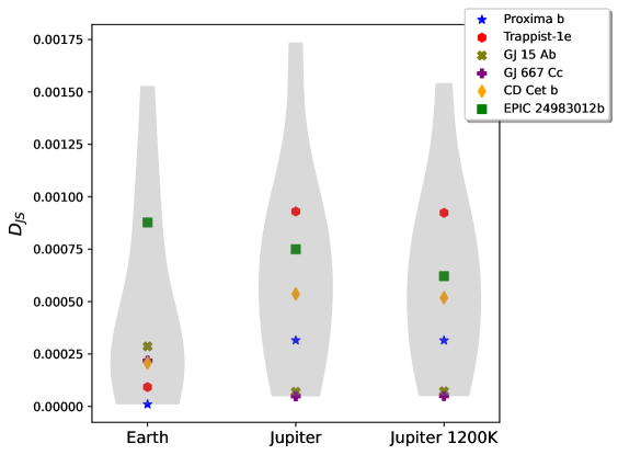
Figure 3: Violin plot showing the $\mathcal{D}_{\rm{JS}}$ distributions comparing the simulated super Earths to Earth (left), to Jupiter (center), and to a Jupiter-clone with the temperature raised to 1200K (right). The width of the violin plot reads like a histogram, indicating the distribution of planets clustered around the mean $\mathcal{D}_{\rm{JS}}$ value. The $\mathcal{D}_{\rm{JS}}$ from observed exoplanets are labeled with colored shapes; remaining points in the $\mathcal{D}_{\rm{JS}}$ distribution are from four exoplanet simulations. Physical parameters for the exoplanets are listed in Table 3.

The super-Earth $\mathcal{D}_{\rm{JS}}$ distributions in Fig. 3 show more general overlap, although different exoplanets (colored shapes) are still clearly distinguished when compared to Earth (left) and to the two Jupiters (center and right). The mean $\mathcal{D}_{\rm{JS}}$ (the bulge in each plot) comparing the super-Earths to Earth is lower than comparing them to Jupiter or to a 1200K Jupiter, although the distributions are less distinct than those comparing hot Jupiters in Fig. 2. Still, when compared to Earth (left plot), with the exception of exoplanet EPIC 24983012b, all others have $\mathcal{D}_{\rm{JS}}$ substantially lower than the hot Jupiters of Fig. 2, indicating that the method distinguishes between the two classes. In particular, we note how Proxima b (blue star) is the closest exoplanet to Earth in this sample. In contrast, EPIC 24983012b has an equilibrium temperature 1200K hotter than Earth and a surface gravity more than twice that of Earth. The high $\mathcal{D}_{\rm{JS}}$ between this exoplanet and Earth indicates that $\mathcal{D}_{\rm{JS}}$ is able to pick up on these physical differences. EPIC 24983012b may be a super Earth, but it is definitely not Earth-like. In general, super Earths have larger radii and typically higher temperatures than Earth, moving them closer to hot Jupiters. Our results are consistent with this.

6 Conclusions

Until recently, the search for other life in the universe has been obstructed by a paucity of data and the complex, unsettled landscape of factors that deem an exoplanet habitable. While JWST and other next generation missions promise to address the first problem, the latter remains. In this paper, we have presented a novel method designed to identify Earth-like planets (and any other kind of planet) that we hope will contribute to a rapid selection of exoplanets with the potential for habitability.

Stephens et al. (2020) and other works cited therein showed that $\mathcal{D}_{\rm{JS}}$ is sensitive to patterns in the data. The better the signal-to-noise ratio and the wavelength resolution of the spectrum, the more efficient the method is. In this work, we have shown that the method can pick up on information encoded in spectral absorption lines. $\mathcal{D}_{\rm{JS}}$ gives a global value for a given spectrum, obtained by summing over all available normalized wavelengths. A wavelength-specific comparison between two spectra is also possible, using the $\mathcal{D}_{\rm{JS}}$-density to zero in on certain chemicals associated with biotic activity, as we will show in a forthcoming work.

The generality of the information-based approach means that it can be used to identify specific exoplanet types, and that it can be rapidly automated by feeding different spectra for comparison. Of course, when searching for biosignatures, the focus is on comparisons between exoplanetary spectra and Earth’s. One of the strengths of this approach is its independence from prior assumptions of what may make an atmosphere Earth-like. Sandford et al. (2021) adopted a similar strategy, demonstrating that patterns in the information of planetary systems can reveal the mass and radius of a missing planet without input physics. Similarly, we contend that the information content of exoplanet atmospheres as encoded in its modal fraction and $\mathcal{D}_{\rm{JS}}$ can help identify exoplanets with potential habitability without the need for prior knowledge of a planet’s physical properties. Indeed, with a large enough database, the information encoded in the spectrum will help elucidate some of these properties (assuming, of course, that the spectrum has sufficient resolution.)

In this paper, we have demonstrated the efficacy of this method using simulated exoplanet data. We first showed that $\mathcal{D}_{\rm{JS}}$ is sensitive to a wide variety of planetary parameters. This indicates that our information measure can be used to identify planetary features. This analysis also showed that $\mathcal{D}_{\rm{JS}}$ is able to differentiate between Earth-like and Jupiter-like planets with reasonable variation in planetary features. To further validate this ability, we used simulations of observed exoplanets - including high-interest exoplanets such as habitable zone planets Trappist-1e and GJ 667 Cc - to show that our method is able to distinguish planet types with realistic data. In both of these illustrations, $\mathcal{D}_{\rm{JS}}$ was able to identify Earth-like and Jupiter-like planets, even without a priori knowledge of what spectral features differentiate the two planet types. This is important, as our limited understanding of the complex scenarios with the potential to host life could cause us to miss habitable planets.

While the $\mathcal{D}_{\rm{JS}}$ distributions comparing super-Earths to Earth, Jupiter, and a warm Jupiter clone showed overlap, we argue that most of the observed super-Earths lie at the low end of the the $\mathcal{D}_{\rm{JS}}$ distribution when compared to Earth but are more spread out when compared to Jupiter and 1200K Jupiter. The overlap in $\mathcal{D}_{\rm{JS}}$ can be greatly reduced by removing the four fabricated super-Earth simulations. The exception - the one observed exoplanet with a high $\mathcal{D}_{\rm{JS}}$ relative to Earth - was EPIC 24983012b, a very large, hot planet. These physical parameters bring the spectrum of the exoplanet closer to a Jupiter or hot Jupiter-like planet than to Earth. The ability of $\mathcal{D}_{\rm{JS}}$ to identify these physical differences in fact underscores our method - EPIC 24983012b is not Earth-like.

Present observations of exoplanetary spectra are limited, using narrow bandpass filters, often with low resolution. As a result, the information content of these spectra is very low. In future work, we hope to use spectra with simulated noise to test the dependence of our method on the signal-to-noise ratio of next generation telescope data. This can be done for JWST using the JWST simulator JexoSim-2.0 (Sarkar & Madhusudhan, 2021), testing the efficacy of the $\mathcal{D}_{\rm{JS}}$ method on JWST data. Ultimately, however, we propose that this method may be used on upcoming high-resolution spectral data from JWST as well as ARIEL, E-ELT, and Earth-2.0. Similar approaches using the information entropic content of a spectrum or a field have been shown to be effective to a wide variety of astrophysical, cosmological, and high-energy physics scenarios: Thakur et al. (2020); Bernardini & da Rocha (2019); Gleiser & Stamatopoulos (2012c, b); Gleiser & Sowinski (2013, 2018); Bernardini et al. (2017); Stephens et al. (2020); Braga & da Rocha (2017) is an incomplete list. To the best of our knowledge, this is the first application of the configurational entropy method to astrobiology.

In closing, as we mentioned above, this method may be extended to determine the information content of individual absorption lines. A companion paper currently in preparation extends the methodology using $\mathcal{D}_{\rm{JS}}$-density to determine the similarity in information between two exoplanets at a particular wavelength. For example, $\mathcal{D}_{\rm{JS}}$ density can be used to compare a particular biosignature signal between an exoplanet spectrum and an Earth spectrum. Used together, $\mathcal{D}_{\rm{JS}}$ and $\mathcal{D}_{\rm{JS}}$-density present a set of information-theory tools for identifying life-supporting exoplanets with minimal prior knowledge.

References

- Anglada-Escudé et al. (2013) Anglada-Escudé, G., Tuomi, M., Gerlach, E., et al. 2013, Astronomy and Astrophysics, 556, A126, doi: 10.1051/0004-6361/201321331
- Barnes et al. (2016) Barnes, R., Deitrick, R., Luger, R., et al. 2016, The Habitability of Proxima Centauri b I: Evolutionary Scenarios, Tech. rep. https://ui.adsabs.harvard.edu/abs/2016arXiv160806919B
- Bauer et al. (2020) Bauer, F. F., Zechmeister, M., Kaminski, A., et al. 2020, Astronomy & Astrophysics, Volume 640, id.A50, pp., 640, A50, doi: 10.1051/0004-6361/202038031
- Benneke et al. (2019) Benneke, B., Wong, I., Piaulet, C., et al. 2019, The Astrophysical Journal Letters, 887, L14, doi: 10.3847/2041-8213/ab59dc
- Bernardini et al. (2017) Bernardini, A. E., Braga, N. R. F., & da Rocha, R. 2017, Physics Letters B, 765, 81, doi: https://doi.org/10.1016/j.physletb.2016.12.007
- Bernardini & da Rocha (2019) Bernardini, A. E., & da Rocha, R. 2019, Physics Letters, Section B: Nuclear, Elementary Particle and High-Energy Physics, 796, 107, doi: https://doi.org/10.1016/j.physletb.2019.07.028
- Birkby (2018) Birkby, J. 2018, Spectroscopic direct detection of exoplanets, ed. H. Deeg & J. Belmonte (Springer), 1485–1508, doi: 10.1007/978-3-319-55333-7_16
- Boyajian et al. (2015) Boyajian, T., von Braun, K., Feiden, G. A., et al. 2015, Monthly Notices of the Royal Astronomical Society, 447, 846, doi: 10.1093/mnras/stu2502
- Braga & da Rocha (2017) Braga, N. R. F., & da Rocha, R. 2017, Physics Letters, Section B: Nuclear, Elementary Particle and High-Energy Physics, 767, 386, doi: https://doi.org/10.1016/j.physletb.2017.02.031
- Charbonneau et al. (2002) Charbonneau, D., Brown, T. M., Noyes, R. W., & Gilliland, R. L. 2002, The Astrophysical Journal, 568, 377, doi: 10.1086/338770
- del Burgo & Allende Prieto (2016) del Burgo, C., & Allende Prieto, C. 2016, Monthly Notices of the Royal Astronomical Society, 463, 1400, doi: 10.1093/mnras/stw2005
- Delrez et al. (2018) Delrez, L., Gillon, M., Triaud, A. H. M. J., et al. 2018, Monthly Notices of the Royal Astronomical Society, 475, 3577, doi: 10.1093/mnras/sty051
- Des Etangs et al. (2008) Des Etangs, A. L., Pont, F., Vidal-Madjar, A., & Sing, D. 2008, Astronomy & Astrophysics, 481, L83, doi: https://doi.org/10.1051/0004-6361:200809388
- Diamond-Lowe et al. (2020) Diamond-Lowe, H., Charbonneau, D., Malik, M., Kempton, E. M. R., & Beletsky, Y. 2020, AJ, 160, 188, doi: 10.3847/1538-3881/abaf4f
- Faedi et al. (2011) Faedi, F., Barros, S. C. C., Anderson, D. R., et al. 2011, Astronomy & Astrophysics, 531, A40, doi: 10.1051/0004-6361/201116671
- Gardner et al. (2006) Gardner, J. P., Mather, J. C., Clampin, M., et al. 2006, Space Science Reviews, 123, 485, doi: https://doi.org/10.1007/s11214-006-8315-7
- Gillon et al. (2009) Gillon, M., Anderson, D. R., Triaud, A. H. M. J., et al. 2009, Astronomy and Astrophysics, 501, 785, doi: 10.1051/0004-6361/200911749
- Gleiser & Sowinski (2013) Gleiser, M., & Sowinski, D. 2013, Physics Letters B, 727, 272, doi: https://doi.org/10.1016/j.physletb.2013.10.005
- Gleiser & Sowinski (2018) —. 2018, Phys. Rev. D, 98, 056026, doi: 10.1103/PhysRevD.98.056026
- Gleiser & Stamatopoulos (2012a) Gleiser, M., & Stamatopoulos, N. 2012a, Physics Letters B, 713, 304, doi: https://doi.org/10.1016/j.physletb.2012.05.064
- Gleiser & Stamatopoulos (2012b) —. 2012b, Physical Review D, 86, doi: 10.1103/physrevd.86.045004
- Gleiser & Stamatopoulos (2012c) —. 2012c, Physical Review D, 86, 045004, doi: 10.1103/PhysRevD.86.045004
- Hartman et al. (2009) Hartman, J. D., Bakos, G. A., Torres, G., et al. 2009, The Astrophysical Journal, 706, 785, doi: 10.1088/0004-637X/706/1/785
- Hidalgo et al. (2020) Hidalgo, D., Pallé, E., Alonso, R., et al. 2020, Astronomy and Astrophysics, 636, A89, doi: 10.1051/0004-6361/201937080
- Kaltenegger (2017) Kaltenegger, L. 2017, Annual Review of Astronomy and Astrophysics, 55, 433, doi: https://doi.org/10.1089/ast.2017.1729
- Kempton et al. (2017) Kempton, E. M.-R., Lupu, R., Owusu-Asare, A., Slough, P., & Cale, B. 2017, Publications of the Astronomical Society of the Pacific, 129, 044402, doi: 10.1088/1538-3873/aa61ef
- Kreidberg et al. (2014) Kreidberg, L., Bean, J. L., Désert, J.-M., et al. 2014, The Astrophysical Journal Letters, 793, L27, doi: https://doi.org/10.1088/2041-8205/793/2/L27
- Kullback & Leibler (1951) Kullback, S., & Leibler, R. A. 1951, The Annals of Mathematical Statistics, 22, 79. https://www.jstor.org/stable/2236703
- Lederberg (1965) Lederberg, J. 1965, Nature, 207, 9, doi: https://doi.org/10.1038/207009a0
- Lin (1991) Lin, J. 1991, IEEE Transactions on Information theory, 37, 145, doi: https://doi.org/10.1109/18.61115
- Lin & Kaltenegger (2020) Lin, Z., & Kaltenegger, L. 2020, Monthly Notices of the Royal Astronomical Society, 491, 2845, doi: 10.1093/mnras/stz3213
- Lissauer et al. (2014) Lissauer, J. J., Dawson, R. I., & Tremaine, S. 2014, Nature, 513, 336, doi: 10.1038/nature13781
- Liu et al. (2014) Liu, F., Asplund, M., Ramirez, I., Yong, D., & Melendez, J. 2014, Monthly Notices of the Royal Astronomical Society: Letters, 442, L51, doi: https://doi.org/10.1093/mnrasl/slu055
- Lovelock (1965) Lovelock, J. E. 1965, Nature, 207, 568, doi: https://doi.org/10.1038/207568a0
- Montañes-Rodriguez et al. (2015) Montañes-Rodriguez, P., Gonzalez-Merino, B., Palle, E., Lopez-Puertas, M., & Garcia-Melendo, E. 2015, The Astrophysical Journal, 801, L8, doi: 10.1088/2041-8205/801/1/L8
- Pinamonti et al. (2018) Pinamonti, M., Damasso, M., Marzari, F., et al. 2018, Astronomy & Astrophysics, 617, A104, doi: 10.1051/0004-6361/201732535
- Ramsay et al. (2020) Ramsay, S., Amico, P., Bezawada, N., et al. 2020, in Advances in Optical Astronomical Instrumentation 2019, Vol. 11203, International Society for Optics and Photonics, 1120303, doi: https://doi.org/10.1117/12.2541400
- Sandford et al. (2021) Sandford, E., Kipping, D., & Collins, M. 2021, Monthly Notices of the Royal Astronomical Society, 505, 2224
- Sarkar & Madhusudhan (2021) Sarkar, S., & Madhusudhan, N. 2021, Monthly Notices of the Royal Astronomical Society, 508, 433, doi: 10.1093/mnras/stab2472
- Sato & Hansen (1979) Sato, M., & Hansen, J. E. 1979, Journal of the Atmospheric Sciences, 36, 1133, doi: 10.1175/1520-0469(1979)036<1133:JACACS>2.0.CO;2
- Schwieterman et al. (2018) Schwieterman, E. W., Kiang, N. Y., Parenteau, M. N., et al. 2018, Astrobiology, 18, 663, doi: https://doi.org/10.1089/ast.2017.1729
- Seager (2013) Seager, S. 2013, Science, 340, 577, doi: https://doi.org/10.1126/science.1232226
- Seager (2014) —. 2014, Proceedings of the National Academy of Sciences, 111, 12634, doi: https://doi.org/10.1073/pnas.1304213111
- Shannon (1948) Shannon, C. E. 1948, Bell System Technical Journal, 27, 623, doi: 10.1002/j.1538-7305.1948.tb00917.x
- Sing et al. (2016) Sing, D. K., Fortney, J. J., Nikolov, N., et al. 2016, Nature, 529, 59, doi: 10.1038/nature16068
- Stephens et al. (2020) Stephens, M., Vannah, S., & Gleiser, M. 2020, Physical Review D, 102, 123514, doi: https://doi.org/10.1103/PhysRevD.102.123514
- Thakur et al. (2020) Thakur, P., Gleiser, M., Kumar, A., & Gupta, R. 2020, Physics Letters A, 384, 126461, doi: https://doi.org/10.1016/j.physleta.2020.126461
- Thompson et al. (2022) Thompson, M. A., Krissansen-Totton, J., Wogan, N., Telus, M., & Fortney, J. J. 2022, Proceedings of the National Academy of Sciences, 119, e2117933119, doi: https://doi.org/10.1073/pnas.2117933119
- Tinetti et al. (2018) Tinetti, G., Drossart, P., Eccleston, P., et al. 2018, Experimental Astronomy, 46, 135, doi: https://doi.org/10.1007/s10686-018-9598-x
- Tinetti et al. (2021) Tinetti, G., Eccleston, P., Haswell, C., et al. 2021, doi: https://doi.org/10.48550/arXiv.2104.04824
- Udry et al. (2014) Udry, S., Lovis, C., Bouchy, F., et al. 2014, arXiv preprint arXiv:1412.1048, doi: https://doi.org/10.17863/CAM.8917
- Ye et al. (2022) Ye, Y., et al. 2022, Nature, 604, 415, doi: https://doi.org/10.1038/d41586-022-01025-2