Multiple change point detection in tensors

Abstract

This paper proposes a criterion for detecting change structures in tensor data. To accommodate tensor structure with structural mode that is not suitable to be equally treated and summarized in a distance to measure the difference between any two adjacent tensors, we define a mode-based signal-screening Frobenius distance for the moving sums of slices of tensor data to handle both dense and sparse model structures of the tensors. As a general distance, it can also deal with the case without structural mode. Based on the distance, we then construct signal statistics using the ratios with adaptive-to-change ridge functions. The number of changes and their locations can then be consistently estimated in certain senses, and the confidence intervals of the locations of change points are constructed. The results hold when the size of the tensor and the number of change points diverge at certain rates, respectively. Numerical studies are conducted to examine the finite sample performances of the proposed method. We also analyze two real data examples for illustration.

Keywords: Adaptive-to-change ridge; Change structure of tensor; Ridge ratio criteria; Signal-screening Frobenius distance; Mode-based signal-screening Frobenius distance

1 Introduction

One of the challenges in the age of big data is heterogeneity. The complexity of the data generation mechanism cannot be fully captured by classical statistical models aimed at studying independent and identically distributed data. Significantly when the data are collected over time, the generation mechanism may change over time, leading to possible structural changes. A commonly adopted assumption is that data structure may only change at times while remaining stationary between two adjacent change points.

This paper focuses on tensor data. Different definitions of structural changes adapt to the nature of applications. For example, Mahyari et al. (2017) identified significant network structure changes with all subjects over time by using the Grassmann distance between the low-rank approximations of two tensors at adjacent times. Their method assumes the normality on the data distribution. Al-Sharoa et al. (2017) constructed two tensors through adjacent matrices and used a Frobenius norm-based normalized cost function to identify change points. Zhan et al. (2021) performed HSI-MSI fusion to obtain high-resolution spectral and spatial images, calculated the differences between the fusion images at two different time points, and used the classification method. Based on the Frobenius distance, the generalized tensor regression method divides the differences into several small tensors. Though empirical successes have been reported, formal theoretical guarantees of the above methods still need to be improved.

For dynamic network data or order-two tensors, Wang et al. (2021) and Zhao et al. (2019) respectively defined the CUSUM-based and MOSUM-based Frobenius distances and chose respective thresholds to identify local maximizers associated with locations of the change points. Both methods need to deal with consistently estimating the sparsity level and choosing thresholds to handle the unknown magnitudes of changes. Specifically, to identify all possible local maximizers associated with the locations of the change points, the thresholds in the MOSUM-based methods proposed by Zhao et al. (2019) and Wang et al. (2021) are related to the unknown minimum magnitude of the changes. Thus, they gave two recommendations for determining the threshold in practice.

We note that in the literature, the Frobenius norm has been popularly used to measure the distance between adjacent data. This distance over all elements of a tensor, including vector and matrix, can successfully summarize the information on changes. On the other hand, various research works have also pointed out that some mode of tensor may represent specific structural information and should be treated separately. The examples include the sensor mode in the seismic Data set of earthquake forecasting (Xie et al. (2019), Chen et al. (2022)), the subject mode in the FMRI data set (Dai et al. (2019)), the sub-region mode in the Brain cancer incidence data set about New Mexico (Kulldorff (2012)), and the spatial grid mode in the data set of the 50-year high-resolution monthly gridded precipitation over Spain (Herrera et al. (2012)). The research interests focus on the significant structural changes with all sensors, subjects/individuals, sub-regions and spatial grids over time respectively. It is thus inappropriate to treat these structural modes equally as other modes in the tensors, as to be summarized in the existing Frobenius distance. To fully leverage the information on the structural mode, our idea in this paper is to first define a new Frobenius-type distance for multiple sub-tensors along the mode, and then take the minimum over all the defined Frobenius distances as the final criterion to detect the heterogeneity of tensors. To achieve this goal, we propose a mode-based signal-screening Frobenius distance over the sub-tensors in this paper. When tensors have no structural mode or there is no need of separately handling structural modes, this general distance can be naturally defined over all elements. Our contributions can be summarized as follows.

First, to adapt dense and sparse model structures automatically, Wang et al. (2021), for the dynamic networks, introduced a notion of sparsity level, but how to consistently estimate this level remains unsolved. We, in this paper, define a novel mode-based signal-screening Frobenius distance between two adjacent tensors in a sequence of the moving sums (MOSUM) as the measure for changes. Fixing the structural mode, the new distance is the averaged Frobenius distance over the remaining signal elements after ruling out those non-signal elements of ‘small’ values of MOSUM (see, e.g., Cho and Fryzlewicz (2015)). The resulting distance becomes a vector. We write it as the MSF-distance in short. This distance can be guarded against being spuriously large, which may cause overestimation when the number of elements is large (see, e.g., Cho and Fryzlewicz (2015)), or spuriously small, which may cause underestimation if the average over its number of elements is considered. As a generic methodology, it can be applied to tensors of order-one (vector), order-two (matrix), and higher-order. Without signal screening in the distance, the distance is then defined over all elements of tensors.

Second, most existing MOSUM-based or CUSUM-based methods rely on the fact that the changes arrive at the maxima and their estimation consistency can be derived when the threshold is properly determined. As the magnitudes of the changes are usually unknown and the threshold depends on the distribution of statistic, its determination is a concern. To circumvent this concern, we define a sequence of ratios between any two adjacent MSF-distances with an adaptive-to-change ridge function. As the resulting sequence is a vector each component having the minima of zero arrived at $z_{k}-2\alpha_{n}+1$, the maxima of infinity arrived at $z_{k}-\alpha_{n}$. Here $z_{k}$’s are the locations of the changes, and $\alpha_{n}$ is the window size of the moving sums. We then define a signal statistic as the minimum of all the components in the vector sequence. The choice of thresholding values can be much more flexible (in theory, any value between 0 and 1 when we search for the minima). The computation can be fast as all change points can be detected simultaneously. The plot of the sequence shows the periodic pattern and can also assist the detection. The estimation consistency for the locations and the number of change points can be derived. Further, we apply a similar idea as in Chen et al. (2021) to construct the confidence intervals of the locations of change points and give more discussion on its construction in Section 3.

Third, in the ratios, we use the adaptive-to-change ridge function to enhance the detection capacity of the criterion compared with a constant ridge as in Zhao et al. (2021) for detecting univariate mean changes. The original purpose of using diminishing ridge is to make the undefined $0/0$ ratios be $1$ such that the detection becomes easy. The adaptive-to-signal ridge function can then go to infinity in the segments without involving change points. Thus, the values of the signal statistic (the empirical version of the sequence mentioned above) can tend to one at a much faster rate than that with a constant ridge so that the curve oscillation at the sample level can be alleviated and false changes could be reduced in practice.

Fourth, in the case with no structural mode and the distance is then naturally defined over all elements of the tensor, the theoretical properties of the criterion will be different. We then separately investigate the distances and the corresponding statistics in two scenarios so that we have two signal statistics.

Fifth, the asymptotic studies on the signal statistic are of theoretical interest. Particularly, when the number of elements in the tensor is not very large, the independent error terms are not required identically distributed, and the second moments are not necessarily identical. These conditions are mild. Although the statistics are empirical versions of their corresponding functions at the population level, inconsistency in some non-negligible segments occurs. Thus, we will give a detailed analysis to identify these segments and study the asymptotic behaviors of the signal statistics in these segments. We will also put an algorithm in Supplementary Materials, which is to prevent the detected change points from falling into these segments so that the estimated number and locations of changes are still consistent. Furthermore, the consistency can be established when the required spacing between any two adjacent change points is shorter than in Zhao et al. (2021) that also used ridge ratios to construct a criterion for mean change detection. We also make some comparison with other methods in the literature for the minimum signal strength and estimation accuracy to see the pros and cons of our method.

The rest of the paper is organized as follows. Section 2 introduces the problem and notion of change point detection in tensors and suggests a criterion to detect change points. As the motivation of the method, we first consider the distance over all elements. Section 3 presents the consistency of the estimated number of changes and the estimated locations in a certain sense. Section 4 includes simulation studies, including the cases with tensors of order-one and higher-order. We find that our method can have better performance in the detection when the number of tensor elements gets larger. This dimensionality blessing phenomenon, particularly in dense cases, might suggest that the dimensionality might not seriously affect the new methods. Section 5 includes the illustrative analyses for two real data examples. Section 6 discusses the merits and limitations of the new method. All other technical proofs and some of numerical studies are included in Supplementary Materials.

2 Methodology Development

2.1 Preliminary

Let $\mathcal{X}_{i}\in\mathbb{R}^{p_{1}\times\cdots\times p_{\kappa}},i=1,2,\cdots,n$ be independent order-$\kappa$ tensors satisfying the model as follows

$$\mathcal{X}_{i} =E(\mathcal{X}_{i})+\mathcal{E}_{i},i=1,2,\cdots,n,$$ (1)

where $\mathcal{E}_{i}$’s are independent error terms with zero mean. Notice that we do not require $\mathcal{E}_{i}$ to be identically distributed or from some specific distributions. Here, the order $\kappa$ is the number of dimensions, and each dimension is called a mode. The element $(i_{1},i_{2},\cdots i_{\kappa})$ of tensor $\mathcal{X}_{i}$ is denoted by $\mathcal{X}_{i,i_{1}i_{2}\cdots i_{\kappa}}$. If we fix the mode-$l$ index of the tensor to be $i_{l}$, then the other $(\kappa-1)$-dimensional sections of a tensor are called the $i_{l}$-th mode-$l$ slice. Thus, a $\kappa$th-order tensor is a $\kappa$-dimensional array with $\kappa$ modes(see more details in Bi et al. (2021), Kolda and Bader (2009) and Venetsanopoulos (2013)).

Assume that there are $K$ change points; that is, $1=z_{0}<z_{1}<\cdots z_{k}<\cdots<z_{K}<z_{K+1}=n$, which divide the original sequence into $K+1$ segments so that

$$E(\mathcal{X}_{i})=\mathcal{M}^{(k)},i=z_{k-1}+1,\cdots,z_{k}.$$

Write $\alpha_{n}^{\star}=\min_{1\leq k\leq K+1}|z_{k}-z_{k-1}|$ as the minimum distance between any two change points. From (1), we can see that the classical change point detection for means (order-one tensor) and covariance matrices (order-two tensor) could be regarded as special cases.

As mentioned in the introduction, our idea is to define a sequence of distances along the structural mode, which eventually form the proposed signal a statistic. But to motivate our method well, we first consider the simple case with no structural mode. Therefore, all modes can be treated equally to define the distance over all elements of the tensor in subsection 2.2 below. The mode-based distance in the general case will be described in subsection 2.3.

2.2 Signal screening distance and a signal statistic

To construct this distance and a signal statistic, we have the following steps.

The moving sums(MOSUM). Define the MOSUM of the tensor sequence as follows:

$$\mathcal{D}(i)=\frac{1}{\alpha_{n}}\left(\sum_{j=i}^{i+\alpha_{n}-1}E(\mathcal{X}_{j})-\sum_{j=i+\alpha_{n}}^{i+2\alpha_{n}-1}E(\mathcal{X}_{j})\right).$$ (2)

As commented before, we define the following signal-screening metric with a threshold $l_{n}(s)\to 0$ as $n\to\infty$:

$$\left|\left|\mathcal{A}\right|\right|_{s}^{2}=\frac{\sum_{i_{1}=1}^{p_{1}}\sum_{i_{2}=2}^{p_{2}}\cdots\sum_{i_{\kappa}=1}^{p_{\kappa}}a_{i_{1}i_{2}\cdots i_{\kappa}}^{2}I(a_{i_{1}i_{2}\cdots i_{\kappa}}^{2}>l_{n}(s))}{\sum_{i_{1}=1}^{p_{1}}\sum_{i_{2}=2}^{p_{2}}\cdots\sum_{i_{\kappa}=1}^{p_{\kappa}}I(a_{i_{1}i_{2}\cdots i_{\kappa}}^{2}>l_{n}(s))+1/n},$$ (3)

where $a_{i_{1}i_{2}\cdots i_{\kappa}}$ denotes $(i_{1},i_{2},\cdots,i_{\kappa})$ element of the $\kappa$-order tensor $\mathcal{A}$ and the value $1/n$ in the denominator is to avoid the undefined $0/0$ ratio. Actually the denominator is to approximate the sparsity of a tensor. When $l_{n}(s)=0$, write $||\mathcal{A}||_{s}^{2}$ as $||\mathcal{A}||_{0s}^{2}$.

In this special case, we call $\|{\cal D}(i)\|_{0s}^{2}$ as the signal screening distance (SF-distance). Some elementary calculations yield the following properties of $||\mathcal{D}(i)||_{0s}^{2}$: for each $1\leq k\leq K$

$$||\mathcal{D}(i)||_{0s}^{2}=\left\{\begin{array}[]{lll}0&&z_{k-1}\leq i<z_{k}-2\alpha_{n}\\ \frac{\sum_{l=1}^{\kappa}\sum_{i_{l}=1}^{p_{l}}\mathcal{D}_{i_{1}i_{2}\cdots i_{\kappa}}^{2}(i)}{\sum_{l=1}^{\kappa}\sum_{i_{l}=1}^{p_{l}}I\left(\mathcal{D}_{i_{1}i_{2}\cdots i_{\kappa}}^{2}(i)>0\right)+1/n}\nearrow&&z_{k}-2\alpha_{n}\leq i<z_{k}-\alpha_{n}\\ ||\mathcal{M}^{(k+1)}-\mathcal{M}^{(k)}||_{0s}^{2}&&i=z_{k}-\alpha_{n}\\ \frac{\sum_{l=1}^{\kappa}\sum_{i_{l}=1}^{p_{l}}\mathcal{D}_{i_{1}i_{2}\cdots i_{\kappa}}^{2}(i)}{\sum_{l=1}^{\kappa}\sum_{i_{l}=1}^{p_{l}}I\left(\mathcal{D}_{i_{1}i_{2}\cdots i_{\kappa}}^{2}(i)>0\right)+1/n}\searrow&&z_{k}-\alpha_{n}<i<z_{k},\\ \end{array}\right.$$

where $\searrow$ and $\nearrow$ are strictly increasing and decreasing, respectively. When there is no change point, $||\mathcal{D}(i)||_{0s}^{2}=0$. When a change comes up, the values of $||\mathcal{D}(i)||_{0s}^{2}$ fluctuate with a length of $2\alpha_{n}$, monotonically increases from $z_{k}-2\alpha_{n}$ to $z_{k}-\alpha_{n}$, taking the maximum at the point $z_{k}-\alpha_{n}$ and then monotonically decreases from $z_{k}-\alpha_{n}$ to $z_{k}$.

Ridge-ratio function. According to the properties of $||\mathcal{D}(i)||_{0s}^{2}$ and $||\mathcal{D}(i+\alpha_{n})||_{0s}^{2}$, we define the ridge ratio statistic at the population level as follows:

$$T(i)=\frac{||\mathcal{D}(i)||_{0s}^{2}+c_{n}^{\star}(i)}{||\mathcal{D}(i+\alpha_{n})||_{0s}^{2}+c_{n}^{\star}(i)},$$ (4)

where the ridge function $c_{n}^{\star}(i)$ to be selected later is to avoid the undefined $0/0$ of $T(i)$ such that $T(i)$ is close to $1$ in the segments where the moving sums in both $||\mathcal{D}(i)||_{0s}^{2}$ and $||\mathcal{D}(i+\alpha_{n})||_{0s}^{2}$ involve no locations of change points. When we use an adaptive-to-change ridge function $c_{n}^{\star}(\cdot)$, Figure 1 presents the curves of $||\mathcal{D}(\cdot)||_{0s}^{2}$ and $T(\cdot)$ for a toy example, showing two very interesting patterns. From the curve of $||\mathcal{D}(\cdot)||_{0s}^{2}$, we can see that each spike uniquely corresponds to a change point. As discussed in Zhao et al. (2019) although $||\mathcal{D}(\cdot)||_{0s}^{2}$ can indicate the locations and number of changes, the unknown magnitudes of the maxima of $||\mathcal{D}(\cdot)||_{0s}^{2}$ brings up the issue of determining a proper threshold. In contrast, the curve of $T(\cdot)$ with local minima of zero and local maxima of infinity can help determine the threshold. Further, different curve patterns of $T(i)$ may occur when the spacings between two adjacent change points are larger than $3\alpha_{n}$, $2\alpha_{n}+f$ or $2\alpha_{n}$, where $f\in(0,\alpha_{n})$. Figure 1 gives the basic idea. More details will be presented in the next section, and the detailed calculation can be found in Supplementary Materials. Briefly speaking, when the spacing is longer than $3\alpha_{n}$, $T(i)$ monotonically decreases on the left-hand side of $z_{k}-2\alpha_{n}+1$, drops to 0 at $z_{k}-2\alpha_{n}+1$, and increases up to infinity. In the last two scenarios, $T(i)$ monotonically decreases to a local minimum first and then suddenly jumps up to one in the interval with length $f+1,0\leq f<\alpha_{n}$, and immediately drops down to another local minimum and follows an up to infinity. All the local minimizers $z_{k}^{\prime}s-2\alpha_{n}+1$ at the right-hand sides of the discontinuous locations in all such intervals correspond to the change points. As the local minima are zero, the threshold for change point detection can be easily determined.

Figure 1: The solid line is for $||\mathcal{D}(i)||_{0s}^{2}$ and the dotted line for $T(i)$.

The adaptive-to-change ridge function. Here, we give the formula of the ridge function for a $\nu>1/2$ and any positive constant $s_{1}$,

$$c_{n}^{\star}(i)=\frac{s_{1}\epsilon_{n}(\log n)^{\nu}}{I(i\in\mathcal{S}^{\star})+\frac{1}{n}}$$ (5)

where $\mathcal{S}^{\star}=\left\{i:\sum_{l=1}^{\kappa}\sum_{i_{l}=1}^{p_{l}}I([\mathcal{D}_{i_{1}i_{2}\cdots i_{\kappa}}(i))]^{2}>0)>0\right\}$ and $\epsilon_{n}=\frac{(\log n)^{\frac{1}{2}+\epsilon}}{\sqrt{\alpha_{n}}}$ that is the uniform rate of $|\mathcal{D}_{n,i_{1},\cdots,i_{\kappa}}(i)-\mathcal{D}_{i_{1},\cdots,i_{\kappa}}(i)|$ over all $\{i_{1},\cdots,i_{\kappa}\}$. The results will be presented in Section 3. First, in the segments involving no locations of changes, the denominator is very small ($1/n$ at the population level); in other words, the ridge tends to infinity such that $T(i)$ tends to one at a fast rate. Second, in the segments involving the locations of changes, $c_{n}^{\star}(i)$ goes to zero with the numerator going to zero and the denominator being larger than $1$. Further, $\mathcal{D}(i+\alpha_{n})$ around the location $z_{k}-2\alpha_{n}$ can be large and $\mathcal{D}(i)$ around $z_{k}-2\alpha_{n}$ can still be small. These lead to small $T(i)$’s around $z_{k}-2\alpha_{n}+1$ such that we can efficiently identify the locations of the changes. We can also use large $T(i)$’s around $z_{k}-\alpha_{n}$ to identify the locations of the change points. But this is similar to using small $1/T(i)$’s. Thus, in this paper, we do not discuss its use.

From Figure 1, we can see that $K$ change points correspond to $K$ disjoint intervals. Thus, we can determine $K$ disjoint intervals by using a thresholding value for $T(\cdot)$. Let $(\tilde{m}_{k}(\tau),\tilde{M}_{k}(\tau))$ denote the intervals where $\tilde{m}_{k}(\tau)$ and $\tilde{M}_{k}(\tau)$ satisfy the following conditions: for a thresholding value $\tau\in(0,1)$, $T(\tilde{M}_{k}(\tau))<\tau\text{ and }T(\tilde{M}_{k}(\tau)+1)\geq\tau,$ and $\tilde{m}_{k}(\tau)=\tilde{M}_{k}(\tau)-\frac{2\sqrt{\tau}}{\sqrt{\tau}+1}\alpha_{n}.$

Use the sample versions of $\mathcal{D}(i)$ and $T(i)$ to define the corresponding signal statistic. Let $\mathcal{D}_{n}(i)=\frac{1}{\alpha_{n}}\left(\sum_{j=i}^{i+\alpha_{n}-1}\mathcal{X}_{j}-\sum_{j=i+\alpha_{n}}^{i+2\alpha_{n}-1}\mathcal{X}_{j}\right)$ and the SF distance-based signal statistic is defined as $T_{n}(i)=\left(||\mathcal{D}_{n}(i)||_{s}^{2}+c_{n}(i)\right)/\left(||\mathcal{D}_{n}(i+\alpha_{n})||_{s}^{2}+c_{n}(i)\right),$ where $c_{n}(i)$ is an estimator of $c_{n}^{\star}(i)$: for a $\nu>1/2$ and any positive constant $s_{1}$,

$$c_{n}(i)=\frac{s_{1}\epsilon_{n}(\log n)^{\nu}}{I(i\in\mathcal{S})+\frac{1}{n}},$$ (6)

and $\mathcal{S}=\left\{i:\sum_{l=1}^{\kappa}\sum_{i_{l}=1}^{p_{l}}I\left(\mathcal{D}_{n,i_{1}i_{2}\cdots i_{\kappa}}^{2}(i)>l_{n}(s)\right)>0\right\}$ is a replacement of $\mathcal{S}^{\star}$ in $c_{n}^{\star}(\cdot)$ where $l_{n}(s)=s\epsilon_{n}(\log n)^{1/2}$, and $s$ and $s_{1}$ are two tuning parameters. Specifically, the thresholding value $0$ in $c_{n}^{\star}(i)$ is replaced by $l_{n}(s)$ such that the set ${\mathcal{S}}^{\star}$ is replaced by $\mathcal{S}$ and $\mathcal{D}(i)$ by $\mathcal{D}_{n}(i)$. Note that the results in Section 3 hold for any $\nu>1/2$, but we recommend $\nu=0.55$, which yields satisfactory performance in all the numerical experiments in Section 4.

Interestingly, as showed in Supplementary Materials, $||\mathcal{D}_{n}(i)||_{s}^{2}$, and $c_{n}(i)$ cannot respectively converge to $||\mathcal{D}(i)||_{0s}^{2}$ and $c_{n}^{\star}(i)$ uniformly over all $i$, which further implies that the sample version $T_{n}(i)$ cannot converge to $T(i)$ uniformly over all $i$. Theorem 3.3 in Section 3 gives the details. Because of the different curve pattern of $T_{n}(\cdot)$ from that of $T(\cdot)$, we will suggest an algorithm to choose the intervals $(m_{k}(\tau),M_{k}(\tau))$ each containing only one local minimizer converging to those of $T(\cdot)$ in a certain sense. The inconsistency occurs in the intervals where $||\mathcal{D}(i)||_{0s}^{2}$ and $||\mathcal{D}(i+\alpha_{n})||_{0s}^{2}$ take small positive values. To help understand this intuitively, we give a toy example in Figure 2. Theorem 3.3 in Section 3 further elaborates when the consistency of $T_{n}(\cdot)$ holds and when it does not, as well as how $T_{n}(\cdot)$ behaves when the consistency does not hold.

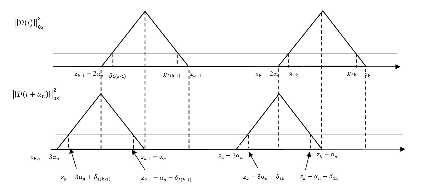
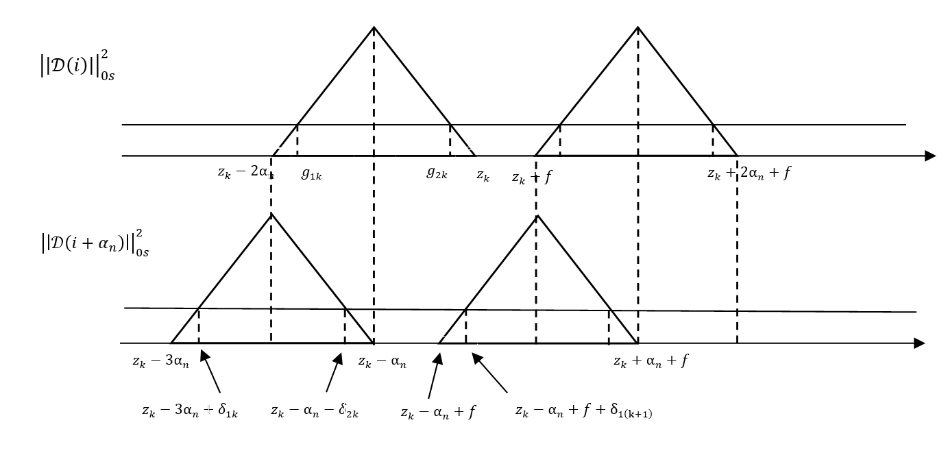
Figure 2: The upper plot is for the case where the distance between two true change points is not less than $3\alpha_{n}$, and the lower plot is about the case where the distance between two true change points is equal to $2\alpha_{n}+f,f\in[0,\alpha_{n})$.

Choosing the intervals.     Motivated by Theorem 3.3 in Section 3, we can, at the sample level, determine the disjoint intervals $(m_{k}(\tau),M_{k}(\tau))$ for $k=1,\cdots,\hat{K}$ that are the estimated intervals of $(\tilde{m}_{k}(\tau),\tilde{M}_{k}(\tau))$’s as follows. First, for a pre-determined threshold $0<\tau<1$, define $M_{k}(\tau)$ by

$$T_{n}(M_{k}(\tau))<\tau,\quad T_{n}(M_{k}(\tau)+1)\geq\tau$$ (7)

and let $m_{k}(\tau)=M_{k}(\tau)-\frac{2\sqrt{\tau}}{\sqrt{\tau}+1}\alpha_{n}$. In this paper, we recommend $\tau=0.8.$ As stated in Theorem 3.3, there might be some $M_{l}(\tau)$’s that correspond to false change points due to the inconsistency of $T_{n}(\cdot)$ in some sets in which we cannot determine the behavior of $T_{n}(\cdot)$. We call them the uncertain sets. Then we rule out those spurious $M_{l}(\tau)$’s when two conditions satisfy: $M_{l+1}(\tau)-M_{l}(\tau)\leq 3\alpha_{n}/2$, and $T_{n}(M_{l}(\tau)-\alpha_{n}/2)\geq 1$, where $l\in\{l:T_{n}(M_{l})\leq\tau\text{ and }T_{n}(M_{l}+1)>\tau\}$. This is because Theorem 3.3 offers two facts: 1). any $M_{l}(\tau)$ corresponding to a false change point has the distance to its nearest $M_{l+1}(\tau)$ corresponding to a true change point should be smaller than $(3-c)\alpha_{n}/2$, and the distance to $M_{l-1}(\tau)$ should be longer than $(3+c)\alpha_{n}/2$ for a small $c>0$; 2). $T_{n}(M_{l}(\tau)-\alpha_{n}/2)\to\infty$.

Identifying the locations of change points.     We can then search for local minimizers in the intervals $(m_{k}(\tau),M_{k}(\tau))$’s with the remaining $M_{k}(\tau)$’s, and use the minimizers plus $2\alpha_{n}-1$ as the estimators $\hat{z}_{k}$’s of $z_{k}$’s. From Figure 1, we can see when the length $f$ is not big (shorter than $\alpha_{n}/2$ in theory), there might exist two or more local minima in one interval (at the population level, there would be exactly two local minima). The distance between one of them plus $2\alpha_{n}-1$ and $z_{k}$ might not be $o(\alpha_{n})$. In other words, if this local minimizer is selected, the estimation consistency is destroyed. To avoid this problem, we set, for $1\leq k\leq\hat{K}$, $r_{k}:=\max\{\arg\min_{i\in(m_{k}(\tau),M_{k}(\tau))}T_{n}(i)\}$ and the estimated location is defined as $\hat{z}_{k}=r_{k}+2\alpha_{n}-1$.

2.3 The mode-based SF distance and a signal statistic

From the above discussion, we can define the mode-based signal screening distance and the corresponding signal statistic. Without loss of generality, we fix the last mode of the tensor to define the slice-wise MOSUM and the corresponding distance. Define, for $1\leq l\leq p_{\kappa}$,

$$\mathcal{D}_{l}(i)= \frac{1}{\alpha_{n}}\left(\sum_{j=i}^{i+\alpha_{n}-1}E(\mathcal{X}_{j,l})-\sum_{j=i+\alpha_{n}}^{i+2\alpha_{n}-1}E(\mathcal{X}_{j,l})\right),$$

where for $1\leq l\leq p_{\kappa}$, $\mathcal{X}_{j,l}\in R^{p_{1}\times p_{2}\times\cdots\times p_{\kappa-1}}$ are the $l$-th slices of the tensor after fixing the $\kappa$-th mode. The corresponding sample versions of $\mathcal{D}_{l}(i)$ and $T_{l}(i)$ are

$$\mathcal{D}_{nl}(i)=\frac{1}{\alpha_{n}}\left(\sum_{j=i}^{i+\alpha_{n}-1}\mathcal{X}_{j,l}-\sum_{j=i+\alpha_{n}}^{i+2\alpha_{n}-1}\mathcal{X}_{j,l}\right)\text{ and }T_{nl}(i)=\frac{||\mathcal{D}_{nl}(i)||_{s}^{2}+c_{nl}(i)}{||\mathcal{D}_{nl}(i+\alpha_{n})||_{s}^{2}+c_{nl}(i)}.$$

Define $T^{v}(i)=\min_{1\leq l\leq p_{\kappa}}T_{l}(i).$ This sequence can identify structural changes at the population level. The final signal statistic based on mode-based SF-distance is defined as $T_{n}^{v}(i)=\min_{1\leq l\leq p_{\kappa}}T_{nl}(i)$. For each $l$, the definition of $c_{nl}(i)$ is similar to $c_{n}(i)$ in (6) with $\mathcal{S}$ being replaced by, for each $1\leq l\leq p_{\kappa}$, $\mathcal{S}_{l}=\left\{i:\sum_{t=1}^{\kappa-1}\sum_{i_{t}=1}^{p_{t}}I\left(\mathcal{D}_{nl,i_{1}i_{2}\cdots i_{\kappa}-1}^{2}(i)>l_{n}(s)\right)>0\right\}.$ Theorem 3.6 in Section 3 offers the estimation consistency of the locations and number of the change points.

Figure 3: the curves of $||\mathcal{D}_{1}(\cdot)||_{0s}^{2}$ and $T^{v}(\cdot)$. The dashed line is for $||\mathcal{D}_{1}(\cdot)||_{0s}^{2}$ and the dot line for $T^{v}(\cdot)$. The upper plot presents the curve when all elements of the vector have changes at the same locations; the lower plot is for the curves when there is at least an element of the vector having changes at different locations.

Write $T^{v}(\cdot)$ and $||\mathcal{D}_{l}(\cdot)||_{0s}^{2}$ as the corresponding functions at the population level. From the two plots of Figure 3 compared with Figure 1, we can see that the curve of $T^{v}(i)$ is different from that of $T(\cdot)$. The top plot shows that if the change points occur in all slices, the curve of $T^{v}(\cdot)$ has the same patten as that of $T(\cdot)$; otherwise, they are different as shown in the bottom plot.

Similarly, to those with $T_{n}(\cdot)$, we also choose the relevant intervals to identify the locations of the local minima.

Choosing the intervals.     By the results of Theorem 3.5 in Section 3, we similarly determine the disjoint intervals $(m_{k}^{v}(\tau),M_{k}^{v}(\tau))$ for $k=1,\cdots,\hat{K}$ as follows. First, for a pre-determined threshold $0<\tau<1$, define $M_{k}^{v}(\tau)$ by

$$T_{n}^{v}(M_{k}^{v}(\tau))<\tau,\quad T_{n}^{v}(M_{k}^{v}(\tau)+1)\geq\tau$$ (8)

and let $m_{k}^{v}(\tau)=M_{k}^{v}(\tau)-\frac{2\sqrt{\tau}}{\sqrt{\tau}+1}\alpha_{n}$. As $T_{n}^{v}(\cdot)$ is the minimum of $T_{nl}(\cdot)$, the values tend to be small at the sample level. We then, in this paper, recommend $\tau=0.4.$ As stated in Theorem 3.5 in the next section, the inconsistency of $T_{n}^{v}(\cdot)$ occurs in the uncertain sets in which we cannot determine what behavior of $T_{n}^{v}(\cdot)$ is. Then, there might also exist some $M_{g}$’s that correspond to false change points. We rule out those $M_{g}$’s when $M_{g+1}(\tau)-M_{g}(\tau)\leq 3\alpha_{n}/2$, where $g\in\{g:T_{n}^{v}(M_{g})<\tau\text{ and }T_{n}^{v}(M_{g}+1)\geq\tau\}$. This is a different algorithm from that with $T_{n}(\cdot)$. It is because Theorem 3.5 offers the fact: any $M_{g}(\tau)$ corresponding to a possible false change point has the distance to its nearest $M_{g+1}(\tau)$ corresponding to a true change point should be smaller than $(3-c)\alpha_{n}/2$, and the distance to $M_{g-1}(\tau)$ should be longer than $(3+c)\alpha_{n}/2$ for a small $c>0$. But we no longer have the property that $T_{n}^{v}(M_{g}(\tau)-\alpha_{n}/2)\to\infty$. See it intuitively from Figure 3.

Identifying the locations of change points.   This step can be similar to that with $T_{n}(\cdot)$ by identifying the local minimizer $r_{k}:=\max\{\arg\min_{i\in(m_{k}^{v}(\tau),M_{k}^{v}(\tau))}T_{n}^{v}(i)\}$ for $1\leq k\leq\hat{K}$ and the estimated location is defined as $\hat{z}_{k}=r_{k}+2\alpha_{n}-1$.

3 The asymptotic properties

This section gives the asymptotic properties of the proposed signal statistics, the estimated locations $\hat{z}_{k}$, and the estimated number $\hat{K}$ of change points. As $T_{n}^{v}(\cdot)$ has different asymptotic behaviors from $T_{n}(\cdot)$, we then also give the results about $T_{n}(\cdot)$ first.

3.1 The asymptotic properties of the SF-distance-based statistic

Introduce some notations to be used in the following theorems. Denote ${\rm{Var}}({\rm{vec}}(\mathcal{E}))=\colon\boldsymbol{\Sigma}=\left(\sigma_{j_{1}j_{2}}\right),1\leq j_{1},j_{2}\leq p$, $p=\prod_{l=1}^{\kappa}p_{l}$ and $p_{-\kappa}=\prod_{l=1}^{\kappa-1}p_{l}$, where ${\rm{vec}}(\cdot)$ represents the vectorization of a tensor. Let $\boldsymbol{\eta}=\boldsymbol{\Sigma^{-\frac{1}{2}}}{\rm{vec}}(\mathcal{E})$, $\boldsymbol{\eta}^{(l)}=\boldsymbol{\Sigma^{-\frac{1}{2}}}{\rm{vec}}(\mathcal{E}_{l})$, $a_{n}=\frac{(logn)^{1+2\epsilon}}{(\log n)^{\rho_{1}}\alpha_{n}\left(\log np\right)}$, and $b_{n}=\frac{(a_{n}\alpha_{n}-2C^{\prime})^{2}}{(\log n)^{\rho_{2}}\log[(K+1)pn](K+1)^{2}}$ for three positive constants $\epsilon$, $\rho_{1}$ and $\rho_{2}$.

Proposition 3.1.

Assume that $\mathcal{X}_{i}-E(\mathcal{X}_{i})$ are independent random tensors.

• Under Condition 1 in Supplementary Materials, when $\frac{n^{2}p}{\alpha_{n}^{4}b_{n}^{2}}\to 0$, we have the following result for the SF-distance-based MOSUM:

  $$\max_{i}\max_{i_{1},i_{2},\cdots,i_{\kappa}}\left|\mathcal{D}_{n,i_{1}i_{2}\cdots i_{\kappa}}(i)-\mathcal{D}_{i_{1}i_{2}\cdots i_{\kappa}}(i)\right|=O_{p}\left(\frac{(\log n)^{\frac{1}{2}+\epsilon}}{\sqrt{\alpha_{n}}}\right).$$ (9)

• Assume that the last mode’s indexes of $\mathcal{X}_{i}$ are independent and the elements $\eta_{ij}$ of $\boldsymbol{\eta}_{i}$ for $i=1,2,\cdots,n;j=1,2,\cdots,p$ are independent and identically distributed. Suppose that Conditions 2 and 3 in Supplementary Materials hold and $\frac{\alpha_{n}^{5}\log\left(np\right)}{n^{4}}=o(1)$. If $\left[E|\eta_{11}|^{q}\right]^{1/q}<\infty\text{ and }\frac{(\log(np))^{3q/2}np}{\alpha_{n}^{q/2}}=o(1)$ hold for some $q\geq 4$, or $E(\exp^{a_{0}\eta_{11}})<\infty\text{ and }\frac{(\log(np))^{\max\{7,2(1+\beta)/\beta\}}}{\alpha_{n}}=o(1)$ for some $a_{0}>0$ hold, then we have the following result for the SF-distance-based MOSUM:

  $$\max_{i}\max_{i_{1},i_{2},\cdots,i_{\kappa}}\left|\mathcal{D}_{n,i_{1}i_{2}\cdots i_{\kappa}}(i)-\mathcal{D}_{i_{1}i_{2}\cdots i_{\kappa}}(i)\right|=O_{p}\left(\frac{\left(\log\left(np\right)\right)^{1/2+\epsilon}}{\sqrt{\alpha_{n}}}\right).$$ (10)

For notational simplicity, denote $\epsilon_{n}=\frac{(\log n)^{\frac{1}{2}+\epsilon}}{\sqrt{\alpha_{n}}}$ in Part (i) and $\epsilon_{n}=\frac{\left(\log\left(np\right)\right)^{1/2+\epsilon}}{\sqrt{\alpha_{n}}}$ in Part (ii).

Remark 1.

(Allowed dimension) This proposition shows the critical differences between Parts (i) and (ii). Particularly, under additional conditions on $\eta_{ij}$, such as the IID condition as well as other conditions on its moment and tail probability (see, e.g., Theorem 1 in Chen et al. (2021)), we can see from Part (ii) that the divergence rate of $p$ can be fast. While when these conditions are relaxed as in Part (i), we still have the estimation consistency of $\mathcal{D}(i)$ with a slower divergence rate of $p$.

In Part (i), the formulas of $a_{n}$ and $b_{n}$ give that

$$\frac{n^{2}p}{\alpha_{n}^{4}b_{n}^{2}}=\frac{n^{2}p(\log n)^{4\rho_{1}+2\rho_{2}}\left[\log\left(np\right)\right]^{4}\left\{\log[(K+1)np]\right\}^{2}(K+1)^{4}}{\alpha_{n}^{4}\left[(\log n)^{1+2\epsilon}-2C^{\prime}(\log n)^{\rho_{1}}\log\left(np\right)\right]^{4}}\to 0.$$

Take $\epsilon=\frac{\rho_{1}}{2}+\frac{\rho_{2}}{4}+1$, then $\frac{n^{2}p\left\{\log[(K+1)n]\right\}^{2}\left[\log(np)\right]^{4}(K+1)^{4}}{\alpha_{n}^{4}[\log n]^{6}}\to 0$. When the number of change points is fixed and $\alpha_{n}=n^{\frac{1}{2}+\nu}$ with $\nu\in(0,\frac{1}{2})$, we can see that $p$ can be close to the order $n^{4\nu}$ and can be close to $n^{2}$ at most. More importantly, we do not require that $\mathcal{X}_{i}-E(\mathcal{X}_{i})$ should be identically distributed or specify that the data come from some specific distribution.

In Part (ii), under the finite moment conditions, $p$ can be at a polynomial order of $n$, depending on $q$. The larger $q$ allows the larger dimension $p$. Under the exponential tail condition, $p$ can be exponential in $n$.

Define $\mathcal{G}=\left\{i:\exists i_{1},i_{2},\cdots,i_{\kappa},\mathcal{D}_{i_{1}i_{2}\cdots i_{\kappa}}^{2}(i)>0\text{ and }\mathcal{D}_{n,i_{1}i_{2}\cdots i_{\kappa}}^{2}(i)\leq l_{n}(s)\right\},$ and $(\mathcal{G}+\alpha_{n})=\{i:i-\alpha_{n}\in\mathcal{G}\}$. Further, let $g_{1k}=\arg\min_{j\in\mathcal{G},j+1\notin\mathcal{G}}|j-(z_{k}-2\alpha_{n})|$ and $g_{2k}=\arg\min_{j\in\mathcal{G},j-1\notin\mathcal{G}}|j-z_{k}|$ for $k=1,2,\cdots,K$.

Proposition 3.2.

Under the conditions in Proposition 3.1, we have

• $\max_{i\in\mathcal{G}^{c}}\big{|}||\mathcal{D}_{n}(i)||_{s}^{2}-||\mathcal{D}(i)||_{0s}^{2}\big{|}=O_{p}(\epsilon_{n})$.

• Let $\delta_{1k}=g_{1k}-(z_{k}-2\alpha_{n})$ and $\delta_{2k}=z_{k}-g_{2k}$. If Condition 6 holds, then $\max_{1\leq k\leq K}\delta_{1k}=o_{p}(\alpha_{n})$ and $\max_{1\leq k\leq K}\delta_{2k}=o_{p}(\alpha_{n})$.

• Let $\mathcal{M}_{n}=\{i:T_{n}(i)\leq M_{n}(i)\}$, where $M_{n}=o\left(\frac{c_{n}(i)}{\epsilon_{n}}\right)$. If Condition 2 holds, $\max_{i\in\mathcal{G}^{c}\cap(\mathcal{G}+\alpha_{n})^{c}\cap\mathcal{M}_{n}}\left|T_{n}(i)-T(i)\right|=o_{p}(1)$.

The above results are the basis for obtaining the consistency of the estimated locations and number of change points when the signal statistic $T_{n}(\cdot)$ is used. There may exist some intervals with length $o(\alpha_{n})$ such that $||\mathcal{D}_{n}(i)||_{s}^{2}$ does not converge to $||\mathcal{D}(i)||_{0s}^{2}$, and similarly for $T_{n}(\cdot)$.

We will, in the following theorem, give some detailed analysis of the inconsistency and some more asymptotic behaviors of $T_{n}(\cdot)$ in the set $\mathcal{G}\cup(\mathcal{G}+\alpha_{n}).$ The proof is included in Supplementary Materials. Importantly, we will show that this set is sufficiently small and does not influence the choice of $M_{k}(\tau)$ and the consistency of $\hat{z}_{k}$.

Note that the inconsistencies of $\mathcal{D}_{n}(\cdot)$, $\mathcal{D}_{n}(\cdot+\alpha_{n})$ and $c_{n}(\cdot)$ in the set $\mathcal{G}\cup(\mathcal{G}+\alpha_{n})$ could cause the inconsistency of $T_{n}(\cdot)$. From the analysis to the set $\mathcal{G}^{c}$ in the Part (i) of Proposition 3.2, we can know that $\mathcal{G}^{c}\subset\{i:c_{n}(i)=c_{n}^{\star}(i)\}$ with a probability going to one. In other words, $\{i:c_{n}(i)\not=c_{n}^{\star}(i)\}\subset\mathcal{G}$ with a probability going to one.

Divide $\mathcal{G}$ into two sets $\mathcal{L}=\mathcal{S}^{\star}\cap\mathcal{S}^{c}$ and $\mathcal{G}\backslash\mathcal{L}$ where $\mathcal{L}$ can be written as

$$\left\{i:\exists i_{1}^{0},i_{2}^{0},\cdots,i_{\kappa}^{0},\mathcal{D}_{i_{1}^{0}i_{2}^{0}\cdots i_{\kappa}^{0}}^{2}(i)>0\text{ and }\forall i_{1},i_{2},\cdots,i_{\kappa},\mathcal{D}_{n,i_{1}i_{2}\cdots i_{\kappa}}^{2}(i)\leq l_{n}(s)\right\}.$$ (11)

Note that $c_{n}(i)=s_{1}n(\log(n))^{\nu}\epsilon_{n}\to\infty,$ for $i\in\mathcal{L}$ defined in (11), and $c_{n}(i)=\frac{s_{1}(\log(n))^{\nu}\epsilon_{n}}{I(i\in\mathcal{S})+\frac{1}{n}}\to 0,$ for $i\in\mathcal{G}\backslash\mathcal{L}$. Further, the set $\mathcal{L}$ also consists of $2K$ disjoint intervals, each containing in the corresponding interval in $\mathcal{G}$. Write $l_{1k}=\arg\min_{j\in\mathcal{L},j+1\notin\mathcal{L}}|j-(z_{k}-2\alpha_{n})|$ and $l_{2k}=\arg\min_{j\in\mathcal{L},j-1\notin\mathcal{L}}|j-z_{k}|$ for $k=1,2,\cdots,K$. Define $l_{1k}-(z_{k}-2\alpha_{n})=\colon\Delta_{1k}$ and $z_{k}-l_{2k}=\colon\Delta_{2k}$. Since $\mathcal{L}\subset\mathcal{G}$, we have $\Delta_{1k}\leq\delta_{1k}$ and $\Delta_{2k}\leq\delta_{2k}$.

Theorem 3.3.

Under the conditions in Proposition 3.2, Conditions 7 and 8 in Supplementary Materials, we have the following results hold with a probability going to $1$.

Case 1. When the distance between two adjacent change points is not less than $3\alpha_{n}$,

• $\min_{k}\min_{i\in(z_{k}-3\alpha_{n},z_{k}-3\alpha_{n}+\delta_{1k}]}T_{n}(i)\to 1$;

• $\min_{k}\min_{i\in(z_{k}-2\alpha_{n},l_{1k}]}T_{n}(i)\to 1$ and $\max_{k}\max_{i\in(l_{1k},g_{1k}]}T_{n}(i)\to 0$;

• $\lim\inf_{n}\min_{k}\min_{i\in[z_{k}-\alpha_{n}-\delta_{2k},z_{k}-\alpha_{n})}T_{n}(i)\geq 1$;

• $\liminf_{n}\min_{k}\min_{i\in[g_{2k},z_{k})}T_{n}(i)\geq 1.$

Case 2.When the distance between two adjacent change points is equal to $2\alpha_{n}+f,f\in[0,\alpha_{n})$,

• $\min_{k}\min_{i\in(z_{k}-2\alpha_{n},l_{1k}]}T_{n}(i)\to 1$ and $\max_{k}\max_{i\in(l_{1k},g_{1k}]}T_{n}(i)\to 0;$

• $\lim\inf_{n}\min_{k}\min_{i\in[z_{k}-\alpha_{n}-\delta_{2k},z_{k}-\alpha_{n})}T_{n}(i)\to 1;$

• $\lim\inf_{n}\min_{k}\min_{i\in(z_{k}-\alpha_{n}+f,z_{k}-\alpha_{n}+f+\delta_{1(k+1)}]\backslash[g_{2k},z_{k})}T_{n}(i)\geq 1;$

• Recall the definition of $M_{k}(\tau)$ in Subsection 2.2. Define $c_{n}=\frac{(\log n)^{\nu}\epsilon_{n}}{1+\frac{1}{n}}$.

  • For $f\in\left[0,\alpha_{n}-\delta_{2k}-\frac{\alpha_{n}\sqrt{A_{2}}}{\min_{k}\min_{\mathcal{H}_{k}}\gamma_{i_{1}i_{2}\cdots i_{\kappa}}^{k}}\right]$, $\max_{k}\max_{i\in[g_{2k},l_{2k})}T_{n}(i)\to 0,$ where $A_{2}=\left[\left(1-\frac{\sqrt{\tilde{l}_{n}(s)}}{\min_{k}\min_{\mathcal{H}_{k}}\gamma_{i_{1}i_{2}\cdots i_{\kappa}}^{k}}\right)\min_{k}\min_{\mathcal{H}_{k}}\gamma_{i_{1}i_{2}\cdots i_{\kappa}}^{k}\right]^{2}.$

  • For $f\in\left[\alpha_{n}-\Delta_{2k}-\frac{\alpha_{n}\sqrt{c_{n}}}{(\log n)^{\frac{1}{8}}\min_{k}\min_{\mathcal{H}_{k}}\gamma_{i_{1}i_{2}\cdots i_{\kappa}}^{k}},\alpha_{n}\right)$, $\lim\inf_{n}\min_{k}\min_{i\in[g_{2k},l_{2k})}T_{n}(i)\geq 1;$

  • For $f\in\left(\alpha_{n}-\delta_{2k}-\frac{\alpha_{n}\sqrt{A_{2}}}{\min_{k}\min_{\mathcal{H}_{k}}\gamma_{i_{1}i_{2}\cdots i_{\kappa}}^{k}},\alpha_{n}-\Delta_{2k}-\frac{\alpha_{n}\sqrt{c_{n}}}{(\log n)^{\frac{1}{8}}\min_{k}\min_{\mathcal{H}_{k}}\gamma_{i_{1}i_{2}\cdots i_{\kappa}}^{k}}\right)$, the set $[g_{2k},l_{2k})$ is an uncertain set in the sense that the convergence is unclear. But, $\lim\inf_{n}\min_{k}\min_{i\in[g_{2k},l_{2k})}T_{n}(i-\frac{\alpha_{n}}{2})\to\infty$ and
    $\lim\sup_{n}\max_{k}\max_{i\in[z_{k}+f,z_{k}+f+\frac{\alpha_{n}}{2}]}T_{n}(i-\frac{\alpha_{n}}{2})\leq 1.$ Further, there is a small value $c>0$ such that

    $$\max_{k}\max_{i\in[g_{2k},l_{2k})}\left|\tilde{M}_{k+1}(\tau)-i\right|<\frac{(3-c)\alpha_{n}}{2}\text{ and }\min_{k}\min_{i\in[g_{2k},l_{2k})}\left|i-\tilde{M}_{k}(\tau)\right|>\frac{(3+c)\alpha_{n}}{2}.$$

  • $\min_{k}\min_{i\in[l_{2k},z_{k})}T_{n}(i)\to 1.$

Remark 2.

The analysis of the results in this theorem is rather tedious. To help understand the results intuitively, we give a toy example to present the set $\mathcal{G}$ in which $\|\mathcal{D}_{n}(i)\|_{s}^{2}$ may not converge to $\|\mathcal{D}(i)\|_{0s}^{2}$, and the set $(\mathcal{G}+\alpha_{n})$. The plots in Figure 2 respectively show the curves in the cases where the distance between two adjacent true change points is not less than $3\alpha_{n}$ and equal to $2\alpha_{n}+f,f\in[0,\alpha_{n})$. We can obviously see that for each $k$, there are four disjoint intervals in $\mathcal{G}$ and $(\mathcal{G}+\alpha_{n})$ discussed in the theorem such that $T_{n}(\cdot)$ may not converge to $T(\cdot)$. When the distance between two adjacent change points is shorter than $3\alpha_{n}$, Part 4 in Case 2 shows that the behavior of $T_{n}(\cdot)$ in some small intervals is very complicated. But the above analysis will help choose the intervals, each containing only one change point in Propostion 6 in Supplementary Materials.

Define $\hat{z}_{k}=0$ if $\hat{K}<k\leq K$.

Theorem 3.4.

Under the conditions in Proposition 3.2, when Conditions 6 and 7 hold in Supplementary Materials, $\alpha_{n}^{\star}\geq 2\alpha_{n}$ and $\frac{n}{K\alpha_{n}^{\star}}\to\infty$, we have $Pr(\hat{K}=K)\to 1,$ and the estimators $\{\hat{z}_{1},\hat{z}_{2},\cdots,\hat{z}_{\hat{K}}\}$ have $\Pr\left\{\max_{1\leq k\leq K}\left|\frac{\hat{z}_{k}-z_{k}}{\alpha_{n}}\right|<\epsilon\right\}\to 1$ for every $\epsilon>0.$

Remark 3.

Theorem 3.4 shows the estimation accuracy of the change point location is of order $o_{p}(\alpha_{n})$ with $\alpha_{n}\gg n^{\frac{1}{2}}p^{\frac{1}{4}}$ in the non-i.i.d. error case (see Proposition 3.1 (i)) or $o_{p}(\alpha_{n})$ with $\frac{\alpha_{n}^{5}\log(np)}{n^{4}}\to 0$ in the i.i.d. error case (see, Proposition 3.1 (ii)). In Supplementary Material, Condition 7 states the minimum signal strength in this paper.

Some comparison with existing results in the literature is in order. Wang et al. (2021) focused on dynamic networks with binary elements, which can be regarded as an order-two tensor. In the i.i.d. error cases its estimation accuracy can achieve the order $o(\alpha_{n}^{\star})$ that is the minimum length between two change points. The constraint $\alpha_{n}^{\star}\geq 2\alpha_{n}$ we require is not assumed in their results, but some other conditions are required. For example, as they commented in their paper (see, Wang et al. (2021), page 210), the denseness in their result requires that more than $O(\sqrt{p})$ elements must change in the same location of any change point. Our method does not need this condition. Further, how to estimate the sparsity is still an unsolved problem in their method. Wang and Samworth (2018) can achieve the accuracy order $o(\sqrt{n})$ that is better than our accuracy order of $o(\alpha_{n})$ in the current paper; but mainly under sparse models and normality.

3.2 The asymptotic properties of the MSF-distance-based statistic

We now analyse $T_{n}^{v}(\cdot)$. Define

$$\mathcal{G}_{l}=\left\{i:\exists i_{1},i_{2},\cdots,i_{\kappa-1},\mathcal{D}_{l,i_{1}i_{2}\cdots i_{\kappa-1}}^{2}(i)>0\text{ and }\mathcal{D}_{nl,i_{1}i_{2}\cdots i_{\kappa-1}}^{2}(i)\leq l_{n}(s)\right\}.$$

Proposition 3.2 also shows the uniform consistency of $\|\mathcal{D}_{nl}(i)\|_{s}^{2}$ to $\|\mathcal{D}_{l}(i)\|_{0s}^{2}$ over the set $\mathcal{G}_{l}^{c}$, while may not be for $i\in\mathcal{G}_{l}$. Thus, according to Proposition 3.3, $T_{nl}(i)$ maintains the uniform consistency over $\mathcal{G}_{l}^{c}\cap(\mathcal{G}_{l}+\alpha_{n})^{c}\cap\mathcal{M}_{nl}$, where $(\mathcal{G}_{l}+\alpha_{n})=\{i:i-\alpha_{n}\in\mathcal{G}_{l}\}$, $\mathcal{M}_{nl}=\{i:T_{n}(i)\leq M_{nl}(i)\}$ and $M_{nl}(i)=o\left(\frac{c_{nl}(i)}{\epsilon_{n}}\right)$.

Recall the definitions of $\mathcal{S}_{l}$ in Subsection 2.4. For notational convenience, write $\mathcal{L}_{l}$ as $\mathcal{S}_{l}^{c}\cap\{i:||\mathcal{D}_{l}(i)||_{0s}^{2}>0\}=\colon\mathcal{S}_{l}^{c}\cap\mathcal{S}_{l}^{\star}$. Similar to the analysis for the signal statistic SFD before Theorem 3.3, the existence of $\mathcal{L}_{l}$ also influences the uniform consistency of $T_{nl}(i)$. As $\mathcal{L}_{l}\subseteq\mathcal{G}_{l}$ that is proved previously, we now use some similar arguments that have been used for each $T_{n}(i)$ to obtain the uniform consistency of $T_{n}^{v}(\cdot)$ over $\mathcal{G}^{vc}\cap(\mathcal{G}^{v}+\alpha_{n})^{c}\cap\mathcal{M}_{n}^{v}$, where $\mathcal{G}^{v}=\cup_{l=1}^{p_{\kappa}}\mathcal{G}_{l}$, $(\mathcal{G}^{v}+\alpha_{n})=\{i:i-\alpha_{n}\in\mathcal{G}^{v}\}$ and $\mathcal{M}_{n}^{v}=\cap_{l=1}^{p_{\kappa}}\mathcal{M}_{nl}$.

Parallel to Theorem 3.3, Theorem 3.5 below shows that $T_{n}^{v}(\cdot)$ has the uniform consistency over $\mathcal{G}^{vc}\cap(\mathcal{G}^{v}+\alpha_{n})^{c}\cap\mathcal{M}_{n}^{v}$, and is inconsistent when $i\in\mathcal{G}^{v}\cup(\mathcal{G}^{v}+\alpha_{n})\cap\mathcal{M}_{n}^{vc}$, but keeps similar properties of $T_{n}(i),i\in\mathcal{G}\cup(\mathcal{G}+\alpha_{n})$ except for Part 4(iii) in Case 2 of Theorem 3.3. Again, the inconsistency of $T_{n}^{v}(i)$ does not influence choosing the disjoint intervals, each containing only one change point, as stated in Proposition 8 in Supplementary Materials.

Now we give some notations that will be used in the following results. Similar to the definitions of $g_{1k}$ and $g_{2k}$ before Proposition 3.2, we define $g_{l,1k}=\arg\min_{j\in\mathcal{G}_{l},j+1\notin\mathcal{G}_{l}}|j-(z_{k}-2\alpha_{n})|$ and $g_{l,2k}=\arg\min_{j\in\mathcal{G}_{l},j-1\notin\mathcal{G}_{l}}|j-z_{k}|$ for $k=1,2,\cdots,K$. Then $\max_{1\leq l\leq p_{\kappa}}g_{l,1k}=\colon g_{1k}^{v}$ and $\min_{1\leq l\leq p_{\kappa}}g_{l,2k}=\colon g_{2k}^{v}$ are the right- and left-hand ending point of $\mathcal{G}^{v}$ respectively. The lengths of $2K$ disjoint intervals in $\mathcal{G}^{v}$ are defined as $g_{1k}^{v}-(z_{k}-2\alpha_{n})=\colon\delta_{1k}^{v}$ and $z_{k}-g_{2k}^{v}=\colon\delta_{2k}^{v},k=1,2,\cdots,K$.

From the proof of Part (ii) in Proposition 3.2 presented in Supplementary Materials, we know that for any $l$, $g_{l,1k}-(z_{k}-2\alpha_{n})=o(\alpha_{n})$ and $z_{k}-g_{l,2k}=o(\alpha_{n})$. Notice that the bound $\sqrt{\tilde{l}_{n}(s)}\alpha_{n}/\min\min_{\mathcal{H}_{k}}\gamma_{i_{1}i_{2}\cdots i_{\kappa}}^{k}$ is free from $l$. Thus, we have $\delta_{1k}^{v}=o(\alpha_{n})$ and $\delta_{2k}^{v}=o(\alpha_{n})$. For $k=1,2,\cdots,K$, write $l_{1k}^{v}=\min_{1\leq l\leq p_{\kappa}}\left\{\arg\min_{j\in\mathcal{L}_{l},j+1\notin\mathcal{L}_{l}}|j-(z_{k}-2\alpha_{n})|\right\}\text{ and }l_{2k}^{v}=\max_{1\leq l\leq p_{\kappa}}\left\{\arg\min_{j\in\mathcal{L}_{l},j-1\notin\mathcal{L}_{l}}|j-z_{k}|\right\}.$ Define $l_{1k}^{v}-(z_{k}-2\alpha_{n})=\colon\Delta_{1k}^{v}$ and $z_{k}-l_{2k}^{v}=\colon\Delta_{2k}^{v}$. Due to $\mathcal{L}_{l}\subseteq\mathcal{G}_{l}$, we have $\Delta_{1k}^{v}\leq\delta_{1k}^{v}$ and $\Delta_{2k}^{v}\leq\delta_{2k}^{v}$.

Similar to the definition of $M_{k}(\tau)$ and $m_{k}(\tau)$, let $M_{k}^{v}(\tau)$ and $m_{k}^{v}(\tau)$ be defined by $T_{n}(M_{k}^{v}(\tau))<\tau$, $T_{n}(M_{k}^{v}(\tau)+1)\geq\tau,\tau\in(0,1)$ and $m_{k}^{v}(\tau)=M_{k}^{v}(\tau)-\frac{2\sqrt{\tau}}{\sqrt{\tau}+1}\alpha_{n}$. $(m_{kl}(\tau),M_{kl}(\tau))$ and $(\tilde{m}_{kl}^{v}(\tau),\tilde{M}_{kl}^{v}(\tau))$ are defined by $T_{n}^{v}(M_{kl}^{v}(\tau))<\tau,T_{n}^{v}(M_{kl}^{v}(\tau)+1)\geq\tau,$ $T^{v}(\tilde{M}_{kl})<\tau,T^{v}(\tilde{M}_{kl}^{v}(\tau)+1)\geq\tau$, and $m_{kl}^{v}(\tau)=M_{kl}^{v}(\tau)-\frac{2\sqrt{\tau}}{\sqrt{\tau}+1}\alpha_{n}$.

Theorem 3.5.

Under the conditions in Proposition 3.2, we have the following results with a probability going to one.

$\bullet$ Additionally, assume Condition 8 in Supplementary Material holds.

Case 1. When the distance between two adjacent change points is not less than $3\alpha_{n}$, for any $k=1,2,\cdots,K$, the union of all the four sets in following Parts 1-4 for all $k=1,2,\cdots,K$ are equal to $\mathcal{G}^{v}\cup(\mathcal{G}+\alpha_{n})^{v}$.

• $\min_{k}\min_{i\in(z_{k}-3\alpha_{n},z_{k}-3\alpha_{n}+\delta_{1k}^{v}]}T_{n}^{v}(i)\to 1$.

• $\min_{k}\min_{i\in(z_{k}-2\alpha_{n},l_{1k}^{v}]}T_{n}^{v}(i)\to 1$ and $\max_{k}\max_{i\in(l_{1k}^{v},g_{1k}^{v}]}T_{n}^{v}(i)\to 0;$

• $\lim\inf_{n}\min_{k}\min_{i\in[z_{k}-\alpha_{n}-\delta_{2k}^{v},z_{k}-\alpha_{n})}T_{n}^{v}(i)\geq 1;$

• $\lim\inf_{n}\min_{k}\min_{i\in[g_{2k}^{v},z_{k})}T_{n}^{v}(i)\geq 1.$

Case 2. When the distance between two adjacent change points is equal to $2\alpha_{n}+f,f\in[0,\alpha_{n})$, the union of all the four sets in following Parts 1-4 for all $k=1,2,\cdots,K$ are equal to $\mathcal{G}^{v}\cup(\mathcal{G}+\alpha_{n})^{v}$.

• $\min_{k}\min_{i\in(z_{k}-2\alpha_{n},l_{1k}^{v}]}T_{n}^{v}(i)\to 1$ and $\max_{k}\max_{i\in(l_{1k}^{v},g_{1k}^{v}]}T_{n}^{v}(i)\to 0;$

• $\lim\inf_{n}\min_{i\in[z_{k}-\alpha_{n}-\delta_{2k}^{v},z_{k}-\alpha_{n})}T_{n}^{v}(i)\geq 1;$

• $\lim\inf_{n}\min_{i\in(z_{k}-\alpha_{n}+f,z_{k}-\alpha_{n}+f+\delta_{1(k+1)}^{v})\backslash[g_{2k}^{v},z_{k})}T_{n}^{v}(i)\geq 1;$

• Recall the definition of $M_{k}^{v}(\tau)$ before this theorem.

  • For $f\in\left[0,\alpha_{n}-\delta_{2k}^{v}-\frac{\alpha_{n}\sqrt{A_{2}}}{\min_{k}\min_{\mathcal{H}_{k}}\gamma_{i_{1}i_{2}\cdots i_{\kappa}}^{k}}\right]$, $\max_{k}\max_{i\in[g_{2k}^{v},l_{2k}^{v})}T_{n}^{v}(i)\to 0;$

  • For $f\in\left[\alpha_{n}-\Delta_{2k}^{v}-\frac{\alpha_{n}\sqrt{c_{n}}}{(\log n)^{\frac{1}{8}}\min_{k}\min_{\mathcal{H}_{k}}\gamma_{i_{1}i_{2}\cdots i_{\kappa}}^{k}},\alpha_{n}\right)$, $\lim\inf_{n}\min_{k}\min_{i\in[g_{2k}^{v},l_{2k}^{v})}T_{n}^{v}(i)\geq 1;$

  • For $f\in\left(\alpha_{n}-\delta_{2k}^{v}-\frac{\alpha_{n}\sqrt{A_{2}}}{\min_{k}\min_{\mathcal{H}_{k}}\gamma_{i_{1}i_{2}\cdots i_{\kappa}}^{k}},\alpha_{n}-\Delta_{2k}^{v}-\frac{\alpha_{n}\sqrt{c_{n}}}{(\log n)^{\frac{1}{8}}\min_{k}\min_{\mathcal{H}_{k}}\gamma_{i_{1}i_{2}\cdots i_{\kappa}}^{k}}\right),$

    $$\max_{k}\max_{i\in[g_{2k},l_{2k})}\left|\tilde{M}_{k+1}^{v}(\tau)-i\right|<\frac{(3-c)\alpha_{n}}{2}\text{ and }\min_{k}\min_{i\in[g_{2k},l_{2k})}\left|i-\tilde{M}_{k}^{v}(\tau)\right|>\frac{(3+c)\alpha_{n}}{2}.$$

  • $\min_{k}\min_{i\in[l_{2k}^{v},z_{k})}T_{n}^{v}(i)\to 1.$

$\bullet$ Furthermore, $\max_{i\in\mathcal{G}^{vc}\cap(\mathcal{G}^{v}+\alpha_{n})^{c}\cap\mathcal{M}_{n}^{v}}\left|T_{n}^{v}(i)-T^{v}(i)\right|=o(1)$.

Because of the similar construction of all elements $T_{nl}(\cdot)$ of $T_{n}^{v}(\cdot)$, the consistency and inconsistency in different sets can be similarly investigated as the above for $T_{n}(\cdot)$. The estimation consistency of the locations and number of change points can still retain. We then do not give the results about $T_{nl}(\cdot)$ while directly stating the asymptotic results about the estimated locations and number of change points when the signal statistic $T_{n}^{v}(\cdot)$ is used.

Theorem 3.6.

Under the conditions in Proposition 3.2, when Conditions 6 and 7 in Supplementary Materials hold, $2\alpha_{n}\leq\alpha_{n}^{\star}$, and $\frac{n}{K\alpha_{n}^{\star}}\to\infty$, the results in Theorem 3.4 hold true with respect to $T_{n}^{v}(\cdot)$.

3.3 A discussion on confidence interval construction

The analysis for confidence interval construction and related issues in Chen et al. (2021) can lead to similar results in our cases without structural mode, which are stated in Theorem 3.7 below. Before presenting the details, we give some notations used for the result.

Denote

$$G_{i,l}=\frac{1}{2\alpha_{n}}\boldsymbol{\Lambda}^{-1}\boldsymbol{\Sigma}^{\frac{1}{2}}\left[I(1\leq i-l\leq\alpha_{n})-I(1\leq l-i\leq\alpha_{n})\right],$$

$\boldsymbol{G}_{i,\cdot}=(G_{i,1},G_{i,2},\cdots,G_{i,n})^{\top}$ and the jump size $\mathcal{M}_{\Delta}^{(k)}\colon=vec(\mathcal{M}^{(k+1)})-vec(\mathcal{M}^{(k)}),k=1,2,\cdots K.$

Define $\mathcal{S}_{k}=\left\{1\leq j\leq p:\mathcal{M}_{\Delta,j}^{(k)}\neq 0\right\}$, where $\mathcal{M}_{\Delta,j}^{(k)}$ is the $j$th coordinate of $\mathcal{M}_{\Delta}^{(k)}$. Further, define $\tilde{\gamma}_{k}=\left((\boldsymbol{\Lambda})^{-1}\mathcal{M}_{\Delta}^{(k)}\right)_{i\in\mathcal{S}_{k}},$ $\tilde{\tilde{\boldsymbol{\Sigma}}}_{k}=(\boldsymbol{\Lambda}^{-1}\boldsymbol{\Sigma}\boldsymbol{\Lambda}^{-1})_{i,j\in\mathcal{S}_{k}},$ $a_{k}=|\tilde{\gamma}_{k}|_{2}^{2}$ and $\zeta_{k}^{2}=\tilde{\gamma}_{k}^{\top}\tilde{\tilde{\boldsymbol{\Sigma}}}_{k}\tilde{\gamma}_{k}$. Note that $W(r)$ is a two-sided Brownian motion, that is, $W(r)=W_{1}(r)$ if $r>0$, and $W(r)=W_{2}(-r)$ if $r<0$, and $W_{1}$ and $W_{2}$ are two independent Brownian motions.

Theorem 3.7.

(The confidence intervals of the locations of change points) Under the conditions in Proposition 3.1 (ii), if $\min_{1\leq k\leq K}\min_{j\in\mathcal{S}_{k}}|(\boldsymbol{\Lambda}^{-1}\mathcal{M}_{\Delta}^{(k)})_{j}|\geq\omega^{+}\gg\sqrt{\frac{\log(np)}{\alpha_{n}}}+\frac{\alpha_{n}}{n}$ and for some constants $\underline{\lambda},\overline{\lambda}>0$, $\underline{\lambda}\leq\lambda_{max}(\boldsymbol{\Lambda}^{-1}\boldsymbol{\Sigma}\boldsymbol{\Lambda}^{-1})/\lambda_{min}(\boldsymbol{\Lambda}^{-1}\boldsymbol{\Sigma}\boldsymbol{\Lambda}^{-1})\leq\overline{\lambda},$ then the confidence interval of $\frac{z_{k}^{\star}}{\alpha_{n}}$ at the level $\alpha$ is $\left(\frac{\hat{z}_{k}-\lfloor\hat{q}_{z,1-\frac{\alpha}{2}}\rfloor-1}{\alpha_{n}},\frac{\tilde{z}_{k}-\lfloor\hat{q}_{z,\frac{\alpha}{2}}\rfloor+1}{\alpha_{n}}\right)$, where $q_{z,1-\frac{\alpha}{2}}$ and $q_{z,\frac{\alpha}{2}}$ are $1-\frac{\alpha}{2}$ and $\frac{\alpha}{2}$th quantiles of the distribution of $\left(\frac{\zeta_{k}}{a_{k}}\right)^{2}\arg\max_{r}\left\{-2^{-1}|r|+W(r)\right\}$ and $\hat{q}_{z,1-\frac{\alpha}{2}}$ and $\hat{q}_{z,\frac{\alpha}{2}}$ are the two estimators of the quantiles.

Remark 4.

We discuss three issues in this remark. First, we can simulate quantiles by Monte Carlo method (Chen et al. (2021)) or derive them from Stryhn (1996) so that the confidence interval can be constructed. Second, note that the above theorem is based on the conditions in Proposition 3.1 (ii). Therefore, the above method may not be feasible under the conditions in Proposition 3.1 (i) as in this case, $\eta_{ij}$ are not i.i.d. and then the limiting distributions may not be derived. This deserves further study. Third, when the mode-based distance is used to detect change points, the confidence intervals would be constructed in practice as follows. According to each change point, we can find a component $T_{nl}$ (though not unique) of $T_{n}^{v}$. Thus, we may use the similar results with respect to the $l$th slice as those in Theorem 3.7 to construct a confidence interval. The details are omitted here.

4 Simulations

To examine the performances of the proposed criterion, we conduct the simulations with several different model settings and compare our methods with existing competing methods, if any. For order-one tensor (vector), we compare with the E-Divisive method (Matteson and James (2014)), the change point detection through the Kolmogorov-Smirnov statistic(Zhang et al. (2017)), the change point detection via sparse binary segmentation(Cho and Fryzlewicz (2015)) and the Inspect method(Wang and Samworth (2018)). The following simulations abbreviate the four methods as ECP, KS, SBS, and Inspect. ECP and KS are implemented in the R package: ECP; SBS and Inspect are respectively implemented in the R packages: hdbinseg and InspectChangepoint and our method is SFD. We only consider our methods for higher-order tensors due to the lack of competitors. In all simulation experiments, $n=1800$, $K=8$ and change point locations are respectively $200,400,600,800,1000,1200,1400,1600$. Each experiment is repeated $N=200$ times to compute the averages of the estimation $\hat{K}$, mean squared error(MSE), and the distribution of $\hat{K}-K$. Also, for the accuracy of the estimated locations, we compute the percentage of “correct” estimations in the replications. Following Cho and Fryzlewicz (2015), the estimated change points lie within the distance of $\lfloor\sqrt{n}/2\rfloor$ from the true change points is considered as the “correct” estimations. We calculate the proportion of all experiments in which at least four true change points were “correctly” estimated, abbreviated as “CP”.

For the case with using the SF distance of MOSUM, we recommend that $\alpha_{n}=\lfloor\frac{2n^{3/4}}{9}\rfloor,$ $\epsilon_{n}=\frac{(\log n)^{0.55}}{\sqrt{\alpha_{n}}},$ $l_{n}(s)=s(\log n)^{1/2}\epsilon_{n}$, and $c_{n}(i)=\frac{s_{1}\epsilon_{n}(\log n)^{0.55}}{I(i\in\mathcal{S})+\frac{1}{n}},$ where $s=2.5s_{1}$ and $s_{1}=1/50$. For the case with using the MSF distance of MOSUM, we recommend $\alpha_{n}=\lfloor\frac{2n^{3/4}}{9}\rfloor,$ $\epsilon_{n}=\frac{(\log n)^{0.55}}{\sqrt{\alpha_{n}}},$ $l_{n}=s(\log n)^{1/2}\epsilon_{n}$, $c_{nl}(i)=\frac{s_{1}\epsilon_{n}n^{0.55}}{I(i\in\mathcal{S}_{l})+\frac{1}{n}}$, $s=10s_{1}$, and $s_{1}=1/50$. Two basis algorithms are listed in Supplementary Materials.

4.1 Order-one tensor

Consider the model: $\boldsymbol{x}_{i}=\boldsymbol{\mu}_{i}+\boldsymbol{\epsilon}_{i},$ where $\boldsymbol{\epsilon}_{i}$ are independent error terms with mean zero, and $p=50;100;500;1,000;2,000$. To save space, we only present the results for $p=50;100;2,000$, and the other results are presented in Supplementary Materials.

Data generating mechanism: The data are segmented into nine parts and come from two distributions whose means are $\boldsymbol{\mu}_{1}$ and $\boldsymbol{\mu}_{2}$ respectively. $\boldsymbol{\mu}^{(i)}=\boldsymbol{\mu}_{1}$ for $i=1,3,5,7,9$ and $\boldsymbol{\mu}^{(i)}=\boldsymbol{\mu}_{2}$ for $i=2,4,6,8$. For space saving, we only present the result of dense case (See, Table 1) and postpone the detailed results about sparse and mixed distribution in Supplementary Materials. For dense case, we consider following cases:

• Strong signals. $\boldsymbol{\epsilon}_{i}\sim\mathcal{\boldsymbol{N}}(\boldsymbol{0},\boldsymbol{I}_{p\times p})$. All of the components of vectors $\boldsymbol{\mu}_{1}$ and $\boldsymbol{\mu}_{2}$ are equal to $1.4$ and $1$ respectively. The magnitude of the signal is then equal to $0.4$.

• Weak signals. $\boldsymbol{\epsilon}_{i}\sim\mathcal{\boldsymbol{N}}(\boldsymbol{0},\boldsymbol{I}_{p\times p})$. The same setting as above except that all of the components of vectors $\boldsymbol{\mu}_{1}$ and $\boldsymbol{\mu}_{2}$ are equal to $1.2$ and $1$ respectively. The magnitude of the signal is $0.2$.

We also tried some other settings, such as the cases with dense (or sparse) and strong signals. Still, elements of the error terms are correlated, and the same settings as sparse and mixed distributions cases, except that all elements are independent. As the comparisons with the other methods show similar observations to those from the above simulations, we then report the detailed results in Supplementary Materials.

Our method is abbreviated as SFD. The basic information from the simulation results is the following. First, SFD performs better with increasing dimensions, regardless of whether the covariance matrix is identity or non-identity. This dimensionality blessing for SFD deserves further study. Second, for all the competitors, the performances are worse when the components of $\boldsymbol{\epsilon}_{i}$ are correlated, and thus, we consider the case with magnitudes being $1$. Third, ECP is a strong competitor, particularly when $p\leq 100$ or $500$. However, SFD computes much faster. Fourth, detection in sparse cases is more difficult than in dense instances. Fifth, SFD has, in comparison with the others, similar performance.

Table 1: Dense case: distribution of $\hat{K}-K$.

$\hat{K}-K$ Scenarios Procedures Means MSE CP $\leq-3$ $-2$ -1 0 1 2 $\geq 3$ Signal=0.4; identity covariance matrix (i)$p=50$ SFD $8.075$ $0.175$ $1$ $0$ $0$ $10$ $165$ $25$ $0$ $0$ ECP $8.080$ $0.080$ $1$ $0$ $0$ $0$ $184$ $16$ $0$ $0$ KS 5.015 10.105 0.395 136 47 14 3 0 0 0 SBS 9.800 4.73 1 0 2 4 21 51 63 59 Inspect 8.115 0.175 1 0 0 0 182 14 3 1 (ii)$p=100$ SFD $8.075$ $0.075$ $1$ $0$ $0$ $0$ $185$ $15$ $0$ $0$ ECP $8.050$ $0.060$ $1$ $0$ $0$ $0$ $191$ $8$ $1$ $0$ KS 4.985 10.155 0.395 144 40 15 1 0 0 0 SBS 9.985 5.115 1 0 0 2 15 47 71 65 Inspect 8.090 0.09 1 0 0 0 182 18 0 0 (iii)$p=2000$ SFD 8.000 0 1 0 0 0 200 0 0 0 ECP $8.045$ $0.045$ $1$ $0$ $0$ $0$ $191$ $9$ $0$ $0$ KS $4.985$ $10.285$ $0.300$ $132$ $55$ $11$ $2$ $0$ $0$ $0$ SBS $9.970$ $5.140$ $1$ $0$ $0$ $2$ $17$ $44$ $79$ $58$ Inspect $8.580$ $1.150$ $1$ $0$ $0$ $0$ $122$ $54$ $14$ $10$ Signal=0.2; identity covariance matrix (i)$p=50$ SFD $7.100$ $1.800$ $0.925$ $15$ $40$ $60$ $80$ $5$ $0$ $0$ ECP $8.075$ $0.105$ $1$ $0$ $0$ $0$ $187$ $12$ $0$ $1$ KS $4.835$ $11.355$ $0.040$ $147$ $38$ $12$ $3$ $0$ $0$ $0$ SBS $9.960$ $5.310$ $0.985$ $0$ $1$ $4$ $18$ $41$ $71$ $65$ Inspect $5.515$ $17.455$ $0.635$ $79$ $24$ $6$ $48$ $34$ $8$ $1$ (ii)$p=100$ SFD $7.950$ $0.400$ $0.975$ $0$ $0$ $35$ $150$ $5$ $10$ $0$ ECP $8.080$ 0.09 1 0 0 0 185 14 1 0 KS $4.850$ $10.970$ $0.020$ $152$ $39$ $8$ $1$ $0$ $0$ $0$ SBS $9.875$ $4.845$ $1$ $0$ $0$ $1$ $19$ $61$ $61$ $58$ Inspect $7.790$ $4.880$ $0.910$ $20$ $9$ $1$ $105$ $39$ $21$ $5$ (iii)$p=2000$ SFD $7.875$ $0.125$ $1$ $0$ $0$ $25$ $175$ $0$ $0$ $0$ ECP $8.065$ $0.075$ $1$ $0$ $0$ $0$ $188$ $11$ $1$ $0$ KS $4.760$ $11.590$ $0.035$ $158$ $29$ $13$ $0$ $0$ $0$ $0$ SBS $10.140$ $5.740$ $1$ $0$ $0$ $0$ $13$ $41$ $72$ $74$ Inspect $9.020$ $3.210$ $1$ $0$ $0$ $0$ $99$ $51$ $24$ $26$

4.2 Higher order tensor

As the literature lacks change point detection methods for general order-two and -three tensors, we only report the simulation results of the two proposed criteria in this paper. Consider the tensor model as

$$\boldsymbol{{X}_{i}}=\boldsymbol{\Sigma_{i}}+\boldsymbol{E_{i}},i=1,2,\cdots,n.$$ (12)

When $\boldsymbol{E}_{i}$ is a random matrix whose elements $E_{i,jk}$ are with means zero, the model is order-two. Consider $p_{2}=kp_{1}$ for $k=1,16.$ Similar observations are made on the simulations with order-three tensors, which are then put in Supplementary Materials.

Data generating mechanism: The data are segmented into nine parts coming from two distributions whose means are $\boldsymbol{\Sigma_{1}}$ and $\boldsymbol{\Sigma_{2}}$ respectively. $\boldsymbol{\Sigma^{(i)}}=\boldsymbol{\Sigma_{1}}$ for $i=1,3,5,7,9$ and $\boldsymbol{\Sigma^{(i)}}=\boldsymbol{\Sigma_{2}}$ for $i=2,4,6,8$.

In the simulations, each row of $\boldsymbol{E_{i}}$ follows $\mathcal{N}(0,\boldsymbol{\tilde{\Sigma})}$ and rows are independent of each other. When $p_{2}=p_{1}$, all elements in $\boldsymbol{\Sigma_{1}}$ and $\boldsymbol{\Sigma_{2}}$ are equal to $1.4$ and $1$, respectively. Here $p_{1}=10,30,50$. The magnitude of the signal is $0.4$. When $p_{2}=16p_{1}$, For $\boldsymbol{\Sigma_{1}}=(\sigma_{ij})$, $\sigma_{ij}=0.8^{|i-j|}$ if $j\leq i$; otherwise, $\sigma_{ij}=1$. All elements in $\boldsymbol{\Sigma_{2}}$ are equal to $1$. Here $p_{1}=10,12$. For space-saving, the cases with all independent elements and order-three tensors are shown in Supplementary Materials.

Table 2: Order-two tensor(row correlation): The distribution of $\hat{K}-K$.

$\hat{K}-K$ Scenario Procedure Mean MSE CP $\leq-3$ $-2$ -1 0 1 2 $\geq 3$ Symmetric cases: $p_{1}=p_{2}$ $p_{1}=10$ MSFD $3.205$ $24.805$ $0.230$ $188$ $9$ $3$ $0$ $0$ $0$ $0$ SFD $8$ $0.430$ $1$ $0$ $3$ $32$ $129$ $34$ $2$ $0$ $p_{1}=30$ MSFD $8.020$ $0.380$ $1$ $0$ $3$ $26$ $136$ $34$ $1$ $0$ SFD $8.005$ $0.005$ $1$ $0$ $0$ $0$ $199$ $1$ $0$ $0$ $p_{1}=50$ MSFD $8.295$ $0.515$ $1$ $0$ $0$ $7$ $140$ $42$ $9$ $2$ SFD $8$ $0$ $1$ $0$ $0$ $0$ $200$ $0$ $0$ $0$ Asymmetric cases: $p_{2}=16p_{1}$ $p_{1}=10$ MSFD $7.365$ $1.825$ $0.765$ $10$ $34$ $67$ $57$ $25$ $6$ $1$ SFD $5.595$ $7.485$ $0.920$ $81$ $69$ $41$ $9$ $0$ $0$ $0$ $p_{1}=12$ MSFD $7.960$ $0.900$ $0.925$ $0$ $14$ $39$ $100$ $36$ $10$ $1$ SFD $7.010$ $1.930$ $0.995$ $15$ $33$ $82$ $70$ $0$ $0$ $0$

The results reported in Table 2 suggest that the symmetric case favors the SFD-based criterion, whereas the asymmetric case with a much large mode favors the mode-based SFD method. This is also the case when the elements of error matrices are independent. See Supplementary Materials.

5 Application

This section gives three real data examples concerned with order-two and order three tensors. We also put the analysis for the order-three tensor data set of video to Supplementary Materials.

5.1 Enron email dynamic network

The CALO project contains data from about $150$ users and their email exchanges. The processed data were used in Priebe et al. (2005), based on $184$ unique addresses over 189 weeks from 1998 to 2002. The data are available in https://www.cis.jhu.edu/~parky/Enron/. We extract the information about the time for sending and receiving emails from each address during the $189$ weeks. We aim to check whether the mail exchange patterns change during this period, reflecting changes in the relationship among these addresses. Each address is regarded as one subject, called the node in networks. The dynamic networks’ adjacency matrix $\boldsymbol{A}_{i},i=1,2,\cdots,188$ reflects the links between any two subjects. If there is an email exchange between subjects $i$ and $j$, the $(i,j)$ element of $\boldsymbol{A}_{i}$ is $1$; otherwise, it is zero.

As this tensor is order-two with $p_{1}=p_{2}$, we first use the SFD-based statistic to detect change points. Three change points are identified at the locations $39$, $94$, and $141$. Thus, the email exchange patterns may change around the July 1999, August 2000 and July 2001. As the sample size is relatively small compared with the size of the tensor, we also use the MSFD-based statistic that identifies the locations $54$, $111$, and $149$, which correspond to November 1999, December 2000 and September 2001.

Priebe et al. (2005) made anomaly detection and identified three weeks $58$th, $94$th and $146$th weeks through their scan statistics with order $0$ and order $1$. These are similar to ours. Galasyn (2002) recorded Enron Chronology and stated the following facts: Enron purchased 5.1 percent of the long-distance gas pipeline company in July 1999 ($54$th week), sham energy deal occured in December 1999 ($58$th week), large-scale insider selling was underway in August 2000 ($94$th week), Enron bought back subsidiary’s publicly held stock in December 2000 ($111$th week), Enron’s stock closed at $46.66$ in July 2001 ($141$th week), Enron CEO made a resignation announcement in September 2001 ($146$th week) and it was announced that Enron restructured itself in September 2001 ($149$th week). Thus, our detection could reflect those changes that happened in Enron.

5.2 Seismic Data

This dataset is retrieved from http://service.ncedc.org/fdsnws/dataselect/1/. It has been analyzed in Xie et al. (2019) and Chen et al. (2022). This dataset contains ground motion sensor measurables recorded from 39 sensors explained that it is important for fusion center to declare an alarm whenever a change point occurs in any sensor. Chen et al. (2022) removed the linear trend and temporal dependence of the data and the processed data are included in R Package ocd. The processed data set contains 14998 observations corresponding to a time from 2.00-2.16am on December 23, 2004 and each observation is a 39-dimensional vector. We have also known a fact that there is an earthquake measured at duration magnitude 1.47Md hit near Atascadero, California at 02:09:54.01. The structural mode consists of 39 sensors, and then we apply MSFD to obtain four change points at $364.352,606.08,637.056$ and $818.176$ corresponding to the time points $02:06:04.352,02:10:06.08,02:10:37.056$ and $02:13:38.176$, respectively. Figure 4 presents the curve of $T_{n}^{v}(\cdot)$.

Figure 4: The plot presents the curve of $T_{n}^{v}(\cdot)$ in seismic data

6 Conclusion

When a structural mode needs to be separately treated, we in this paper propose a general mode-based signal-screening Frobenius distance (MSFD) of MOSUM. so that we can handle dense and sparse scenarios. When all modes can be equally treated, this distance is reduced to be a signal-screening Frobenius distance (SFD) of MOSUM. The defined criterion is based on ratios of MSFD’s with adaptive-to-signal ridge functions to enhance the detection capacity. The method has several advantages: estimation consistency, robustness against distribution and sparsity structure, computational simplicity, and visualization. Its limitations are mainly in two aspects. We require that the distance between any two changes cannot be too small and the performances of the criterion are relatively sensitive to the choices of $s_{1}$ in the ridge and $s$ in the threshold in the distance. These deserve further study.

SUPPLEMENTARY MATERIAL

Supplemenraty of Multiple change point detection of tensor Conditions, proofs of theoretical results and some additional numerical studies . (.pdf file)

References

- Al-Sharoa et al. (2017) Al-Sharoa, E., M. Al-Khassaweneh, and S. Aviyente (2017). A tensor based framework for community detection in dynamic networks. In 2017 IEEE international conference on acoustics, speech and signal processing (ICASSP), pp. 2312–2316. IEEE.
- Bi et al. (2021) Bi, X., X. Tang, Y. Yuan, Y. Zhang, and A. Qu (2021). Tensors in statistics. Annual review of statistics and its application, 345–368.
- Chen et al. (2021) Chen, L., W. Wang, and W. B. Wu (2021). Inference of breakpoints in high-dimensional time series. Journal of the American Statistical Association, 1–13.
- Chen et al. (2022) Chen, Y., T. Wang, R. J. Samworth, et al. (2022). High-dimensional, multiscale online changepoint detection. Journal of the Royal Statistical Society Series B 84, 234–266.
- Cho and Fryzlewicz (2015) Cho, H. and P. Fryzlewicz (2015). Multiple-change-point detection for high dimensional time series via sparsified binary segmentation. Journal of the Royal Statistical Society: Series B (Statistical Methodology) 77, 475–507.
- Dai et al. (2019) Dai, M., Z. Zhang, and A. Srivastava (2019). Discovering common change-point patterns in functional connectivity across subjects. Medical image analysis 58, 101532.
- Galasyn (2002) Galasyn, J. (2002). ’enron chronology’. https://desdemonadespair.net/2010/09/bushenron-chronology.html.
- Herrera et al. (2012) Herrera, S., J. M. Gutiérrez, R. Ancell, M. Pons, M. Frías, and J. Fernández (2012). Development and analysis of a 50-year high-resolution daily gridded precipitation dataset over spain (spain02). International Journal of Climatology 32, 74–85.
- Kolda and Bader (2009) Kolda, T. G. and B. W. Bader (2009). Tensor decompositions and applications. SIAM review 51, 455–500.
- Kulldorff (2012) Kulldorff, M. (2012). Brain cancer incidence in new mexico. http://www.satscan.org/datasets/nmbrain/index.html.
- Mahyari et al. (2017) Mahyari, A. G., D. M. Zoltowski, E. M. Bernat, and S. Aviyente (2017). A tensor decomposition-based approach for detecting dynamic network states from eeg. IEEE Transactions on Biomedical Engineering 64, 225–237.
- Matteson and James (2014) Matteson, D. S. and N. A. James (2014). A nonparametric approach for multiple change point analysis of multivariate data. Journal of the American Statistical Association 109, 334–345.
- Priebe et al. (2005) Priebe, C. E., J. M. Conroy, D. J. Marchette, and Y. Park (2005). Scan statistics on enron graphs. Computational & Mathematical Organization Theory 11, 229–247.
- Stryhn (1996) Stryhn, H. (1996). The location of the maximum of asymmetric two-sided brownian motion with triangular drift. Statistics & Probability Letters 29, 279–284.
- Venetsanopoulos (2013) Venetsanopoulos, A. (2013). -fundamentals of multilinear subspace learning. In Multilinear Subspace Learning, pp. 78–99. Chapman and Hall/CRC.
- Wang et al. (2021) Wang, D., Y. Yu, and A. Rinaldo (2021). Optimal change point detection and localization in sparse dynamic networks. The Annals of Statistics 49, 203–232.
- Wang and Samworth (2018) Wang, T. and R. J. Samworth (2018). High dimensional change point estimation via sparse projection. Journal of the Royal Statistical Society: Series B (Statistical Methodology) 80, 57–83.
- Xie et al. (2019) Xie, L., Y. Xie, and G. V. Moustakides (2019). Asynchronous multi-sensor change-point detection for seismic tremors. In 2019 IEEE International Symposium on Information Theory (ISIT), pp. 787–791. IEEE.
- Zhan et al. (2021) Zhan, T., Y. Sun, Y. Tang, Y. Xu, and Z. Wu (2021). Tensor regression and image fusion-based change detection using hyperspectral and multispectral images. IEEE Journal of Selected Topics in Applied Earth Observations and Remote Sensing 14, 9794–9802.
- Zhang et al. (2017) Zhang, W., N. A. James, and D. S. Matteson (2017). Pruning and nonparametric multiple change point detection. In 2017 IEEE international conference on data mining workshops (ICDMW), pp. 288–295. IEEE.
- Zhao et al. (2021) Zhao, W., X. Zhu, and L. Zhu (2021). Detecting multiple change points: the pulse criterion. Statistica Sinica Accepted.
- Zhao et al. (2019) Zhao, Z., L. Chen, and L. Lin (2019). Change-point detection in dynamic networks via graphon estimation. arXiv preprint arXiv:1908.01823.