A New Order Parameter for the Higgs Transition in
$SU(2)$-Higgs Theory

Abstract

We investigate the Higgs transition within the four dimensional $SU(2)-$ gauge-Higgs model in search for an order parameter as a function of the Higgs field hopping parameter, $\kappa$, using Lattice technique. We measure the Higgs condensate after applying Landau Gauge Fixing and study the corresponding susceptibility, magnetization and fourth order Binder cumulant using four different spatial volumes with $N_{\tau}\!=\!2$. The computation is carried out with gauge coupling, $\beta_{g}\!=\!8$, for a range of scalar self-coupling, $\lambda\!=\!\{0.00010,0.00350\}$, with emphasis near the critical end-point. Finite size scaling analysis of the gauge fixed condensate and its cumulants agree with the standard $3$d Ising values $\nu=0.62997$, $\beta/\nu=0.518$, $\gamma/\nu=1.964$ at $\lambda=0.00150$. These results are in agreement with previous studies suggesting $3$d Ising universality class. The numerical results also indicate that, at the transition point, the gauge fixed condensate vanishes in the infinite volume limit.

I Introduction

The understanding of the phase structure of $SU(2)-$Higgs theory has crucial cosmological and experimental consequences Kuzmin:1985mm ; Matveev:1988pj ; Rubakov:1996vz ; Fodor:1998if . Over the years, several non-perturbative lattice studies have been devoted in this regard Damgaard:1986qe ; Evertz:1986af ; Bunk:1992xt ; Farakos:1994xh ; Kajantie:1995kf ; Rummukainen:1998as ; Bunk:1992kf ; Bunk:1994xs ; Kajantie:1996mn ; Gurtler:1997hr ; Gurtler:1997ki ; Buchmuller:1994qy ; Karsch:1996aw ; Karsch:1996yh ; Fodor:1994dm ; Fodor:1994sj ; Csikor:1995jj ; Aoki:1996cu ; Aoki:1999fi ; Bonati:2009pf ; DOnofrio:2014rug ; DOnofrio:2015gop ; DOnofrio:2012yxq ; Laine:2012jy ; Gould:2022ran (For reviews, please see Kajantie:1994mt ; Jansen:1995yg ; Rummukainen:1996sx ). These studies find that the nature of Higgs transition varies with Higgs quartic coupling ($\lambda$). With increase in $\lambda$, the strength of this transition weakens and eventually becomes a crossover for large $\lambda$. The $1$st order transition and crossover regions are separated by a $2$nd order critical end-point at $\lambda_{c}$ Aoki:1999fi . There are similar examples in QCD, spin-models, condensed matter systems etc. where lines/surfaces of second order transition that separate $1$st order and crossover regions in the phase diagram Pisarski:1983ms ; Karsch:2000xv ; Alonso:1993tv . Many attempts have been made to study the universality class of such critical end-points in different theories Pisarski:1983ms ; Alonso:1993tv ; Rummukainen:1998as ; Karsch:2000xv . These end-points are expected to belong to the universality class of the Ising model Alonso:1993tv ; Rummukainen:1998as ; Janke:1996qb ; Karsch:2000xv ; Wilding:1994zkq ; Wilding:1994ud ; Wilding:1996 ; Rehr:1973zz . In the electroweak theory, the critical end-point in dimensionally reduced $SU(2)-$Higgs theory is studied in three dimensions Rummukainen:1998as . The analysis of the critical behavior is done by identifying energy and magnetization like observables Alonso:1993tv . The distribution of these observables, higher cumulants and the extracted critical exponents, clearly show that the end-point is in the $3$d Ising universality class.

In ref. Rummukainen:1998as , a linear combinations of various gauge invariant observables plays the role of magnetization. Another orthogonal linear combination plays the role of energy like observable. These linear combinations change with the bare parameters of the theory. Though gauge invariant observables can be used to study nature of transitions, it is desirable to have an order parameter for the Higgs transition. In the absence of gauge symmetry, the Higgs condensate (volume average of the Higgs field) plays the role of an order parameter. On other hand, gauge symmetry renders the condensate unphysical. However, it can be made well behaved by a suitable choice of a gauge. It is expected that the choice of a gauge will not affect physical quantities such as critical exponents. Note that the necessity of a suitable order parameter exists in other gauge theories, such as in high density QCD to describe the normal to color superconducting transition.

In the present work, we propose that the Higgs condensate in the Landau gauge, denoted by $\Phi^{g}$, as an order parameter for the Higgs transition in $SU(2)-$Higgs theory. In $3+1$ dimensions, $\Phi^{g}$ and its cumulants are computed using Monte Carlo simulation of the partition function by varying the Higgs hoping parameter ($\kappa$) and the quartic coupling. It is observed that the partition function average of $\Phi^{g}$ behaves similar to that of magnetization in spin models. For small $\lambda$, the Higgs transition is of $1$st order, and $\Phi^{g}$ is found to vary discontinuously across the transition point. With the increase in $\lambda$, the Higgs transition weakens which is also seen in $\Phi^{g}$ behavior. The jump in $\Phi^{g}$ across the transition point decreases with $\lambda$. At a critical point $\lambda_{c}$, $\Phi^{g}$ varies continuously while its various cumulants show singular behavior. The observed scaling behavior is consistent with $3$d Ising universality class and deviates from the universality class of the $3$d $O(4)$ spin models Kanaya:1994qe ; Toussaint:1996qr . The Finite Size Scaling (FSS) of $\Phi^{g}$ suggests that it vanishes at the critical point in the infinite volume limit. It also vanishes in the high temperature or Higgs symmetric phase at least for $\lambda<\lambda_{c}$. We would like to mention here that $\Phi^{g}$, as an order parameter, reasonably reproduces the previous results. A linear combination along the lines of previous studies may further fine tune the results.

The draft is organized as follows. In Sec. II, we provide the lattice definition of the $SU(2)$-Higgs theory. In Sec. III, we discuss the numerical procedures for our work. This includes the Landau Gauge Fixing in Lattice. In Sec. V, we analyze our data using FSS, while we present the magnetization study at various $\lambda$’s in Sec. VI. Finally, we present the discussion and conclusion of our study in Sec. VII.

II Lattice Formalism

The continuum action of $SU(2)$ gauge-Higgs theory is discretized in Lattice as,

$$\displaystyle S = \sum_{x}\left[\sum_{\mu>\nu}\frac{\beta}{2}\,\mbox{Tr}\,U_{x,\mu\nu}+\sum_{\mu}\kappa\,\mbox{Tr}\,\left(\phi^{\dagger}_{x}\,U_{x,\mu}\,\phi_{x+{\hat{\mu}}}\right)-\frac{1}{2}\,\mbox{Tr}\left(\phi^{\dagger}_{x}\phi_{x}\right)-\lambda\left(\frac{1}{2}\,\mbox{Tr}\left(\phi^{\dagger}_{x}\phi_{x}\right)-1\right)^{2}\right]\,,$$

where $U_{x,\mu}\in SU(2)$ is a link variable, and $U_{x,\mu\nu}$ is a product of four link variables which form a plaquette, and $\phi_{x}$ is $2\otimes 2$ matrix in isospin space describing the Higgs scalar field. The bare parameters $\beta_{g}\equiv 4/g^{2}$ is the gauge coupling, $\lambda$ is the scalar quartic coupling, and $\kappa$ is the scalar hopping parameter which is related to the bare mass square by the relation, $\mu^{2}_{0}=(1-2\lambda)\,\kappa^{-1}-8$.

In order to search for an order parameter, we apply Landau gauge fixing, $\partial_{\mu}\,A_{\mu}\!=\!0$, and construct the condensate, $\Phi^{g}$. We then study the behavior of the magnetization, susceptibility and fourth order Binder cumulant of $\Phi^{g}$ (defined below) at various values of $\kappa$ and $\lambda$ while $\beta_{g}\!=\!8$ is kept fixed.

Magnetization $$: \hskip 14.22636pt\Phi^{g}\,\equiv\,\langle\tilde{\Phi}^{g}\rangle\,=\,\left\langle\frac{1}{N_{s}^{3}N_{t}}\sqrt{\sum_{i=1}^{4}\left(\displaystyle\sum_{x}\phi^{g}_{i,x}\right)^{2}}\right\rangle,$$ (2)

$$\mbox{Susceptibility,}\,\,\chi^{c}\hskip 14.22636pt : \hskip 14.22636ptV\,\left(\langle{\tilde{\Phi}^{g}}{}^{2}\rangle-\langle\tilde{\Phi}^{g}\rangle^{2}\right),$$ (3)

$$\mbox{Total Susceptibility,}\,\,\chi\hskip 14.22636pt : \hskip 14.22636ptV\,\langle{\tilde{\Phi}^{g}}{}^{2}\rangle,$$ (4)

$$\mbox{Binder Cumulant,}\,\,B_{4}\hskip 14.22636pt : \hskip 14.22636pt1-\frac{\langle{\tilde{\Phi}^{g}}{}^{4}\rangle}{3\,\langle{\tilde{\Phi}^{g}}{}^{2}\rangle^{2}}.$$ (5)

where $\langle\cdots\rangle$ stands for gauge average, and $V=N_{s}^{3}$ is the spatial volume of the lattice. We use the superscript, $c$, in Eq. (3) to specify it as the Connected Susceptibility.

We devote a significant part of our study near the end-point for $1$st order transition, namely at $\lambda=0.00116,0.00132$ and $0.00150$. Note that the first value of $\lambda$ is found to be the critical end-point in Ref. Aoki:1999fi . The two higher $\lambda$ values lie around $\sim+2\sigma$ of the first one. The reason to include these higher values of $\lambda$ is discussed in the Sec. V.1. We list the run parameters in Table 1.

III Numerical Procedure and Parameters

For Monte Carlo simulations, we use the pure gauge part of the publicly available MILC code milc and modify it to accommodate the Higgs fields. To update the gauge fields, we first use the standard heat bath algorithm Creutz:1980zw ; Cabibbo:1982zn , and then update Higgs fields using pseudo heat bath algorithm Bunk:1994xs . We then again update the gauge fields using $4$ overrelaxation steps Whitmer:1984he after which Higgs fields are updated again using pseudo heat bath algorithm. To reduce auto-correlation between successive configurations, we carry out $50$ cycles of this updating procedure between two subsequent measurements. We test our codes to reproduce histogram profiles similar to Ref. Aoki:1996cu . For our simulations, we use four spatial volumes, $N_{s}\!=\!20,24,32,40$ while the temporal lattice extent is kept at $N_{\tau}=2$ Aoki:1999fi .

To implement Landau gauge fixing, we maximize the following quantity

$$H = \displaystyle\sum_{x}\sum^{4}_{\mu=1}\mbox{Re}\,\left[\mbox{Tr}\,U_{x,\mu}\right]\,.$$ (6)

In order to maximize $H$, we separately apply two different methods as described in Aoki:2003ip . One of the methods is the standard $SU(2)$ subgroup method, and the other one is Overrelaxed Steepest Descent method. This was done to check whether both the methods arrive at the same global maxima. In addition, we use single, double and quadruple precisions in our simulations so that we are able to set our convergence conditions accordingly. We find that both the methods for maximization of $H$ as well as the different precisions produce similar results. Eventually, as described in Aoki:2003ip , we combine both $SU(2)$ subgroup and Overrelaxed Steepest Descent methods to speed up gauge fixing. First, we apply $SU(2)$ subgroup method to bring the configuration close to the maximum, and then apply Overrelaxed Steepest Descent method for the final convergence. We set our overrelaxation parameter, $\omega=1.98$, and we use double precision for all our simulations. For convergence of $SU(2)$ subgroup method, we measure

$$h \sim \frac{H}{N^{3}_{s}\,N_{\tau}},$$ (7)

We set the convergence condition at the $i$th iteration as,

$$\left|h_{i}-h_{i-1}\right| < 10^{-12}\,.$$ (8)

For the Steepest Descent method, we measure

$$\Delta = \displaystyle\frac{1}{N^{3}_{s}\,N_{\tau}}\sum_{x}\frac{1}{2}\sum^{4}_{\mu=1}\frac{1}{4}\,\mbox{Tr}\,\left[\Delta_{x,\mu}\Delta^{\dagger}_{x,\mu}\right],$$ (9)

where

$$\Delta_{x,\mu} = U_{x-\hat{\mu},\mu}-U_{x,\mu}-\mbox{h.c.}-\mbox{trace}\,.$$ (10)

We set the convergence condition for $\Delta_{j}$ at the $j$th iteration as,

$$\left|\Delta_{j}\right| < 10^{-15}.$$ (11)

Simulations are performed for a wide range of $\kappa$ and $\lambda$ values. We focus our studies at $\lambda\!=0.00116,0.00132$ and $0.00150$. For each of them, we generate $2.5$ million trajectories out of which gauge fixing is performed on every $50$-th trajectory at each $\kappa$. This gives us a total $50\,000$ gauge-fixed configurations for each $\kappa$. The parameters are listed in Table 1. For each of other values of $\lambda$, we generate $500\,000$ trajectories instead out of which every $50$-th trajectory is selected for gauge fixing giving $10\,000$ gauge-fixed configurations for each $\kappa$. The reduced statistics is due to the limitations in computational resources. The parameters are listed in Table 2. All the error analyses in this study are carried out using Jackknife method with bin size determined such a way that the total number of bins is $100$.

Table 1: Simulation parameters near $\lambda_{c}$.

$\beta_{g}$	$\lambda$	$N_{s}$	$N_{\tau}$	$\kappa$	Confs.	Trajectories
						between
						consecutive
						confs.
8.0	0.00116	20, 24, 32, 40	2	{0.129390, 0.129550}	50 000	50
	0.00132	20, 24, 32, 40	2	{0.129420, 0.129820}	50 000	50
	0.00150	20, 24, 32, 40	2	{0.129500, 0.130000}	50 000	50

IV $M$-like and $E$-like observables

The $SU(2)-$Higgs theory is similar to the case of the liquid-gas system, i.e none of the gauge invariant observables can be directly identified with the $M$-like and $E$-like observables. In the previous studies of the critical endpoint, observables such as $S_{K}=\displaystyle\sum_{x,\mu}\mbox{Tr}\left(\phi^{\dagger}_{x}\,U_{x,\mu}\,\phi_{x+{\hat{\mu}}}\right)$, $S_{\phi}=\displaystyle\sum_{x}\left(\frac{1}{2}\,\mbox{Tr}\ \left(\phi^{\dagger}_{x}\phi_{x}\right)-1\right)^{2}$ etc. have been used to define the $M$-like and $E$-like observables. It has been pointed out that $S_{K}$, $S_{\phi}$ etc. are not necessarily orthogonal in the vicinity of the critical point, i.e. $\langle\Delta S_{K}\Delta S_{\phi}\rangle\neq 0$ where $\Delta S_{K}=S_{K}-\langle S_{K}\rangle$ and $\Delta S_{\phi}=S_{\phi}-\langle S_{\phi}\rangle$ Rummukainen:1998as ; Alonso:1993tv ; Karsch:2000xv ; Wilding:1994zkq ; Wilding:1994ud ; Wilding:1996 . However, linear and orthogonal combinations of them have been found to behave as $M$-like and $E$-like observables. In the present work, we include the Landau gauge fixed Higgs condensate, $\Phi^{g}$, along with other gauge invariant observables to define $M$-like and $E$-like observables. The studies of correlations between $\Phi^{g}$ and other gauge invariant observables seem to suggest that $\langle\Delta\Phi^{g}\Delta S_{K}\rangle\approx 0$ and $\langle\Delta\Phi^{g}\Delta S_{\phi}\rangle\approx 0$, are satisfied within the uncertainties.

We compute the correlation relations, $\langle\Delta\Phi^{g}\Delta S_{K}\rangle$ and $\langle\Delta\Phi^{g}\Delta S_{\phi}\rangle$, over the whole range of respective $\kappa$ values at $\lambda=0.00116$ and $0.00150$. They are plotted in Figs. 1 and 2, respectively. We clearly see that there is no correlation between the $\Phi^{g}$ and other observables. We also observe that the sizes of uncertainties decrease as the volume increases. This suggests that $\Phi^{g}$ is a $M$-like observable.

We also study the behaviour of the $\Phi^{g}$ distributions vs. $S_{K}$ as well as $S_{\phi}$ distributions. In Fig. 3, we plot $\Phi^{g}$ vs. $S_{K}$ and $S_{\phi}$ for $\lambda=0.00116$ and $\kappa=0.129465$. In Fig. 4, the same quantities are plotted for $\lambda=0.001500$ and $\kappa=0.129765$. From these figures, we see that these distributions behave similarly to those of energy vs. magnetization distributions of the $3$d Ising Model. Note that $\Phi^{g}$ has four components. The individual components have no physical significance, as there are no Goldstone modes in this case. The magnitude of $\Phi^{g}$ is physical and as a consequence, we can only reproduce the part of the Ising model figure for which $M>0$. In Figs. 3 and 4, we observe that the distributions are not linear, unlike the distribution of $S_{k}$ vs. $S_{\phi}$. In this situation, no unique linear combination is possible.

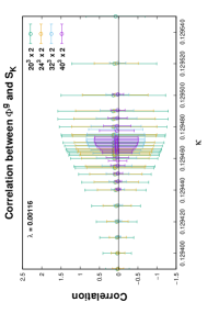
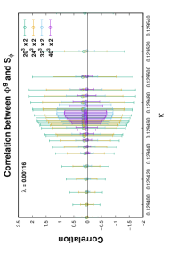
Figure 1: Correlations between (a) $\Phi^{g}$ and $S_{K}$ (b) $\Phi^{g}$ and $S_{\phi}$ at $\lambda=0.00116$.

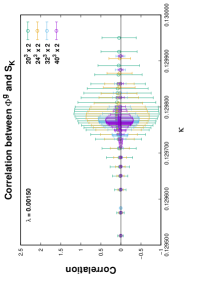
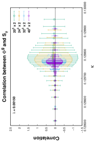
Figure 2: Correlations between (a) $\Phi^{g}$ and $S_{K}$ (b) $\Phi^{g}$ and $S_{\phi}$ at $\lambda=0.00150$.

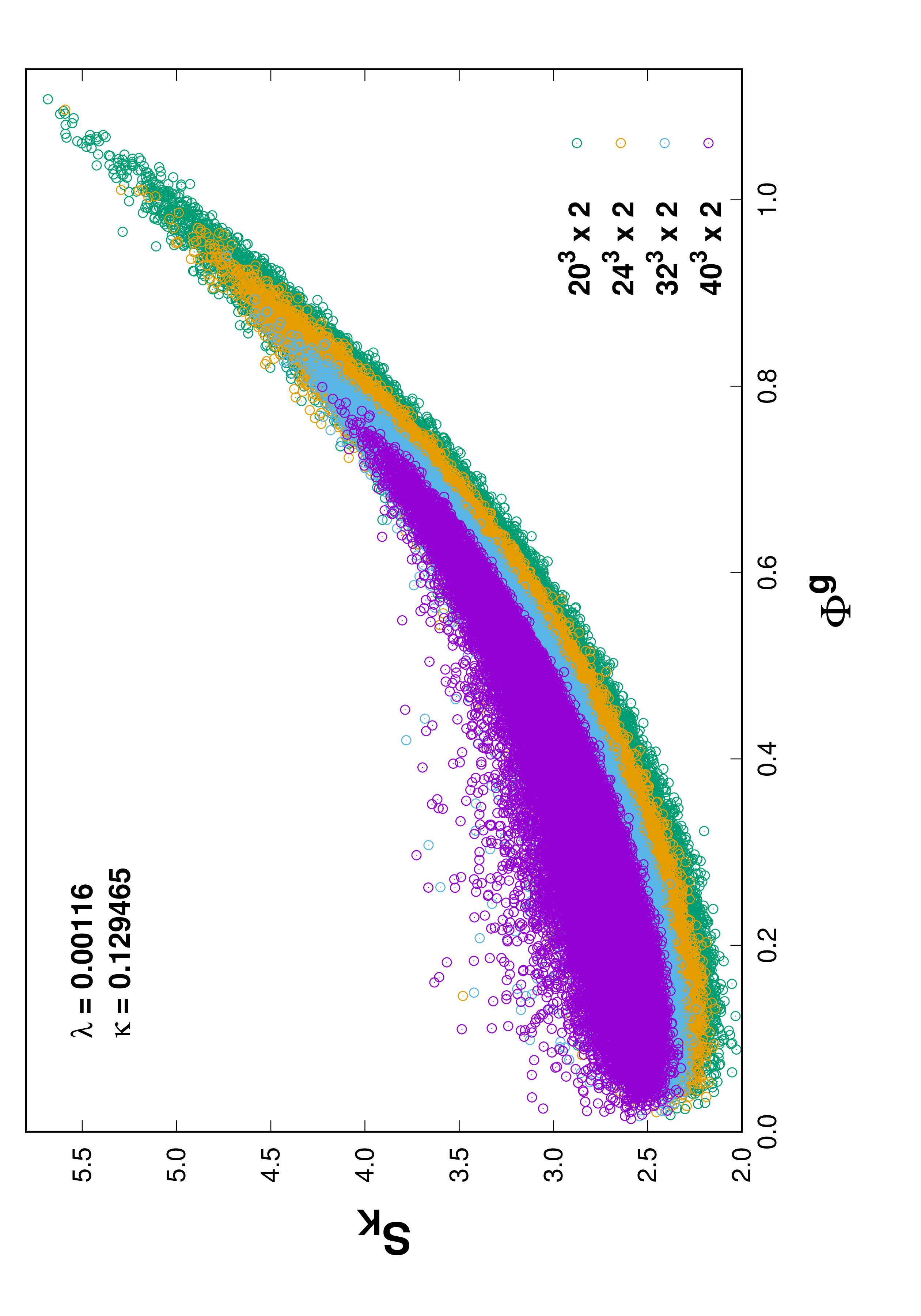
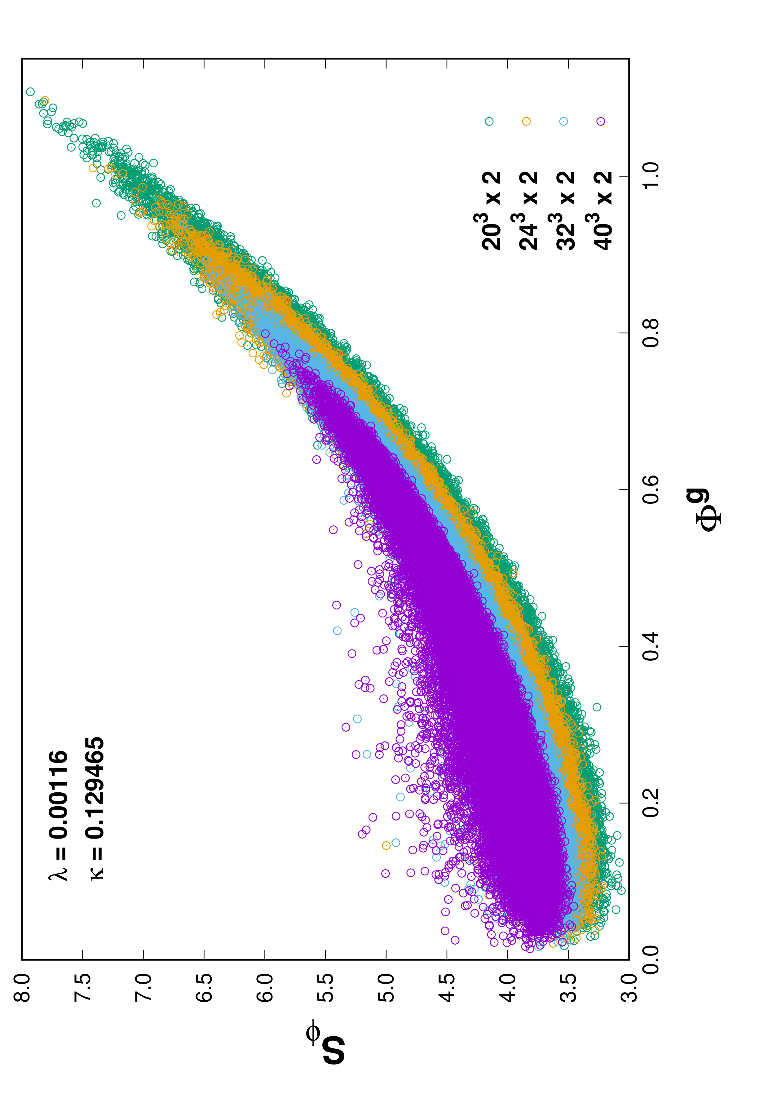
Figure 3: $\Phi^{g}$ vs. (a) $S_{K}$ and (b) $S_{\phi}$ at $\lambda=0.001160$ and $\kappa=0.129465$.

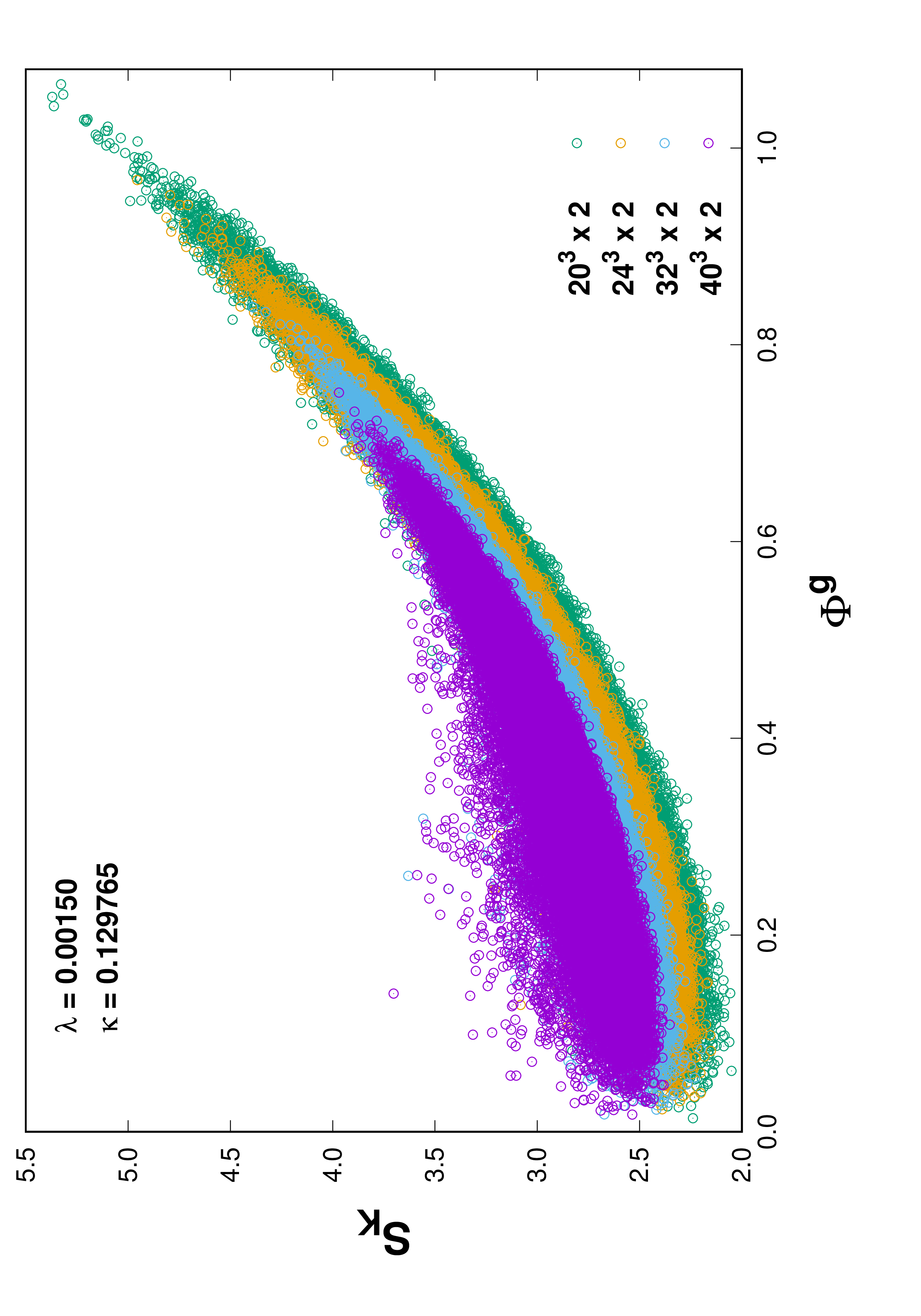
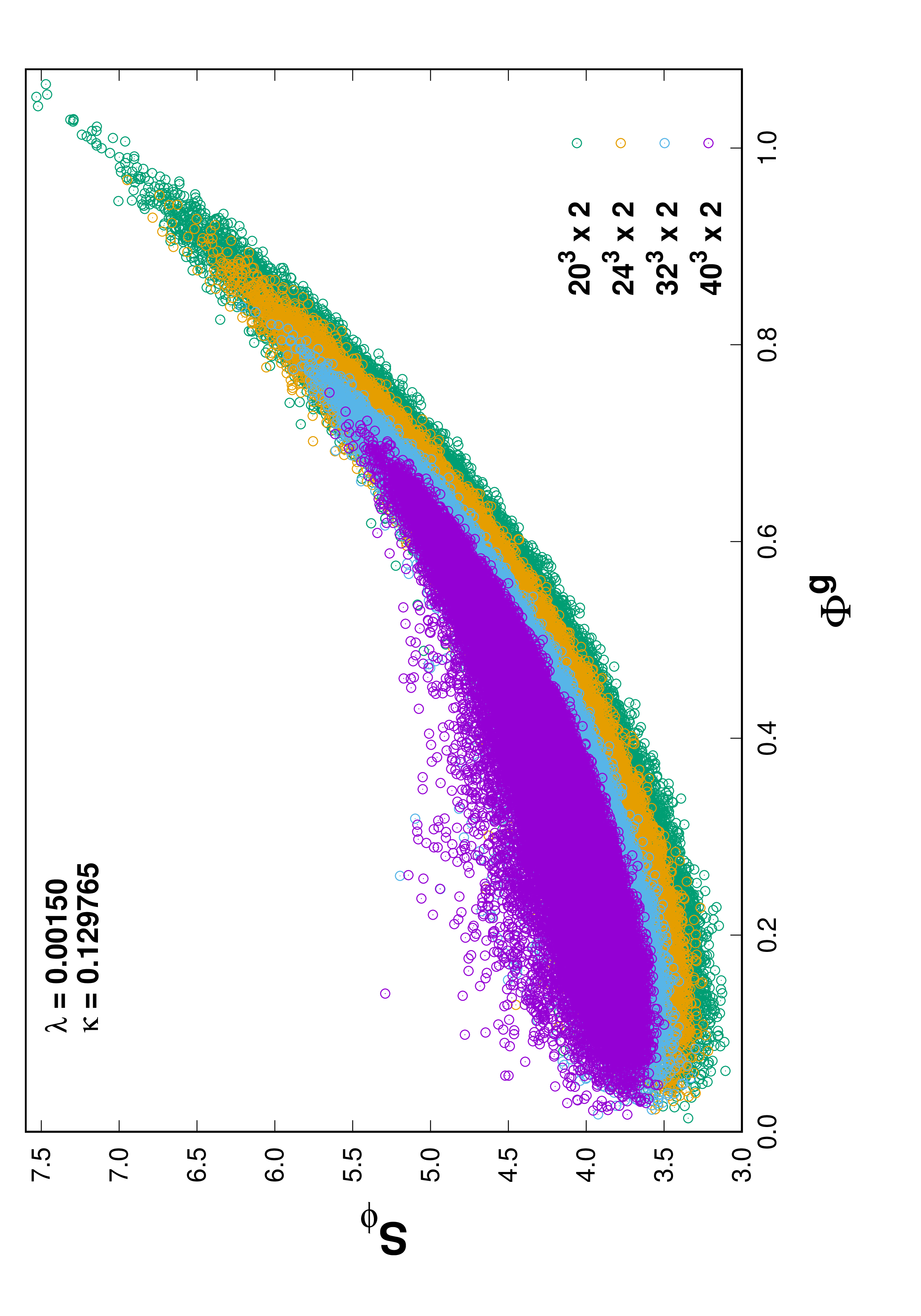
Figure 4: $\Phi^{g}$ vs. (a) $S_{K}$ and (b) $S_{\phi}$ at $\lambda=0.001500$ and $\kappa=0.129765$.

V Finite Size Scaling Analysis

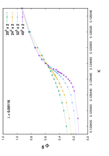
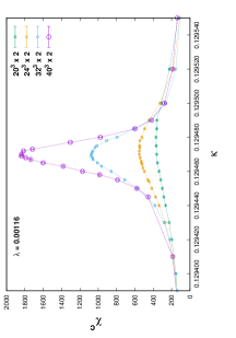
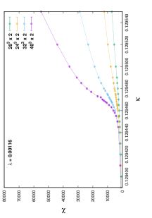
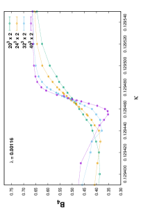
Figure 5: (a) Magnetization (b) Connected susceptibility (c) Total susceptibility, and (d) Binder cumulant as functions of $\kappa$ at $\lambda=0.00116$. The dotted lines are not fitted and are for eye guides only.

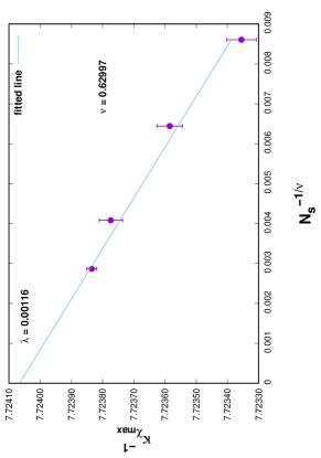
Figure 6: The values of ${\kappa_{\chi}}_{\mbox{\scriptsize max}}$ as a function of $N_{s}^{-1/\nu}$ at $\lambda=0.00116$ for $N_{s}=20,24,32$ and $40$. We set $\nu=0.629971$. The intersection of the fitted straight line provides the value of $\kappa_{c}$.

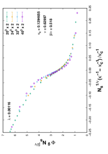
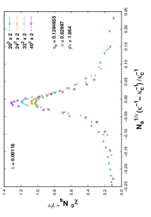
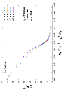
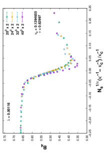
Figure 7: Scaled (a) Magnetization (b) Connected susceptibility (c) Total susceptibility, and (d) Binder cumulant as functions of $\kappa$ at $\lambda=0.00116$.

V.1 $\lambda=0.00116$

In Fig. 5, we plot magnetization, susceptibility, total susceptibility and Binder cumulant for $\lambda=0.00116$. We see that $\kappa$ acts like an “inverse temperature” Wurtz:2009gf for all the four quantities, and there are indications that these four quantities behave similar to that of Ising Model. However, it is necessary to study further by scaling all the four quantities with the standard Ising exponents and see whether the scaled quantities follow the FSS behavior.

In order to carry out the scaling procedure, the corresponding critical value of $\kappa$ needs to be evaluated. To find $\kappa_{c}$, we first estimate the value of $\chi^{c}_{\mbox{\scriptsize max}}$ for each volume and obtain the corresponding ${\kappa_{\chi}}_{\mbox{\scriptsize max}}$. The standard procedure to find $\chi^{c}_{\mbox{\scriptsize max}}$ is the Rewieghting method. It can be seen from Fig. 5 that we have a reasonable amount of data near the peak point for every volume. Thus, we instead use the Cubic Spline Interpolation method to generate a few hundred points close to ${\kappa_{\chi}}_{\mbox{\scriptsize max}}$ for every Jackknife sample. From these sets of interpolated points, we find the values of $\chi^{c}_{\mbox{\scriptsize max}}$ and the corresponding ${\kappa_{\chi}}_{\mbox{\scriptsize max}}$ for each volume. The value of $\kappa_{c}$ is then obtained by using the following FSS relation given by,

$${\kappa_{\chi}}_{\mbox{\scriptsize max}}^{-1} = \kappa_{c}^{-1}+a\,N_{s}^{-1/\nu}.$$ (12)

By using the standard value of $\nu=0.629971$ for $\!3$d Ising Model, we get the value of $\kappa_{c}$ from the linear fit of ${\kappa_{\chi}}_{\mbox{\scriptsize max}}$ as a function of $N_{s}^{-1/\nu}$ as (See Fig. 6),

$$\kappa_{c} = 0.1294655(5).$$ (13)

Using the value of $\kappa_{c}$ from Eq. (13), and the standard $\!3$d Ising values of $\gamma=1.237075$ and $\beta=0.326419$, the quantities are scaled. They are plotted in Fig. 7.

It can be clearly seen from Fig. 7 that quantities do not properly obey the scaling behavior. The differences are more visible in the cases of susceptibility and Binder cumulant. Further, no improvement in the scaling is seen by changing the universality class. We thus extend our study to other $\lambda$ values for which scaling can be seen. We considered two other values of $\lambda$, namely $\lambda=0.00132$ and $0.00150$, which are around $\sim 1\sigma$ and $\sim 2\sigma$ from $\lambda=0.00116$, respectively.

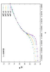
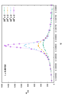
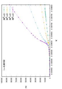
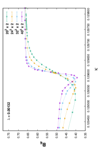
Figure 8: (a) Magnetization (b) Connected susceptibility (c) Total susceptibility, and (d) Binder cumulant as functions of $\kappa$ at $\lambda=0.00132$. The dotted lines are for eye guides only.

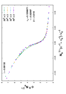
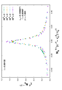
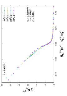
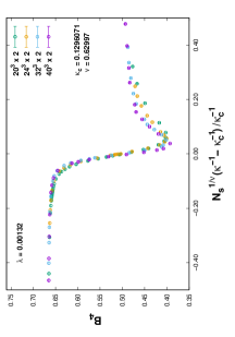
Figure 9: Scaled (a) Magnetization (b) Connected susceptibility (c) Total susceptibility, and (d) Binder cumulant as functions of $\kappa$ at $\lambda=0.00132$.

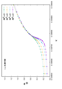
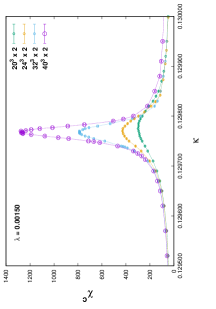
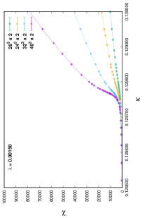
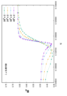
Figure 10: (a) Magnetization (b) Connected susceptibility (c) Total susceptibility, and (d) Binder cumulant as functions of $\kappa$ at $\lambda=0.00150$. The dotted lines are for eye guides only.

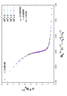
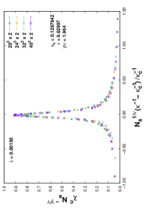
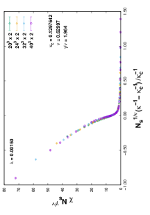
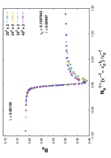
Figure 11: Scaled (a) Magnetization (b) Connected susceptibility (c) Total susceptibility, and (d) Binder cumulant as functions of $\kappa$ at $\lambda=0.00150$.

V.2 $\lambda=0.00132$ and $0.00150$

We compute magnetization, susceptibility, total susceptibility and Binder cumulant for $\lambda=0.00132$ and $0.00150$. They are plotted in Figs. 8 and 10, respectively. We again see Ising like behavior of these quantities. Note that the value of $\kappa_{c}$ changes with the value of $\lambda$. We follow the same procedure as described in Sec. V.1 to determine $\kappa_{c}$ for $\lambda=0.00132$ and $0.00150$. Thus, we get,

$$\kappa_{c} = 0.1296071(8)\,\,\,\,\,\mbox{for $\lambda=0.00132$},$$ (14)

$$\kappa_{c} = 0.1297642(7)\,\,\,\,\,\mbox{for $\lambda=0.00150$}.$$ (15)

Using these values of $k_{c}$ and the standard values of the exponents for $\!3$d Ising Model, we scale the quantities as in Sec. V.1. They are plotted in Figs. 9 and 11, respectively. By comparing Figs. 7, 9 and 11, we see scaling for $\lambda=0.00150$. This is an indication that $\Phi^{g}$ is a good order parameter. Also this suggests that the critical end-point is close to $\lambda=0.00150$.

VI Magnetization at various other $\lambda$’s

Table 2: Run parameters for other $\lambda$’s.

$\beta_{g}$	$\lambda$	$N_{s}$	$N_{\tau}$	$\kappa$	Confs.	Trajectories
						between
						consecutive
						confs.
8.0	0.00010	20, 24, 32, 40	2	{0.127800, 0.128890}	10 000	50
	0.00050	20, 24, 32, 40	2	{0.127800, 0.129200}	10 000	50
	0.00080	20, 24, 32, 40	2	{0.129000, 0.129400}	10 000	50
	0.00095	20, 24, 32, 40	2	{0.129000, 0.129400}	10 000	50
	0.00100	20, 24, 32, 40	2	{0.129120, 0.129500}	10 000	50
	0.00170	20, 24, 32, 40	2	{0.129690, 0.130300}	10 000	50
	0.00220	20, 24, 32, 40	2	{0.129450, 0.130600}	10 000	50
	0.00270	20, 24, 32, 40	2	{0.130000, 0.131340}	10 000	50
	0.00310	20, 24, 32, 40	2	{0.129500, 0.135000}	10 000	50
	0.00350	20, 24, 32, 40	2	{0.127500, 0.137000}	10 000	50

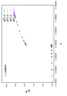
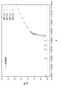
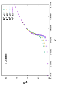
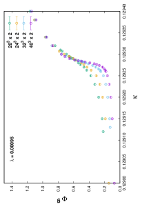
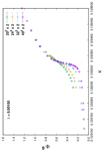
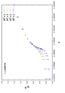
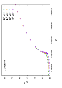
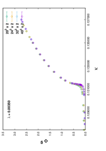
Figure 12: Magnetization at various values of $\lambda$. (a) $\lambda=0.00010$, (b) $\lambda=0.00050$, (c) $\lambda=0.00080$, (d) $\lambda=0.00095$, (e) $\lambda=0.00100$, (f) $\lambda=0.00170$, (g) $\lambda=0.00310$, and (h) $\lambda=0.00350$.

We further investigate whether $\Phi^{g}$ displays the behavior of a conventional order parameter as a function of $\lambda$. We study the magnetization for various $\lambda$ values between $\{0.0001,0.0035\}$. The simulation parameters for this study are listed in Table 2. As mentioned in Sec. III, the number of configurations is restricted to $10\,000$ only for each combination of $\lambda$ and $\kappa$.

From Figs. 12 and 12 at $\lambda=0.00010$ and $0.00050$, respectively, we clearly see that $\Phi^{g}$ displays a $1$st order transition as a function of $\kappa$. Finally, we see from Figs. 12 and 12 that the volume dependence nearly disappears at the values of $\lambda=0.00310$ and $0.00350$, respectively, indicating a cross-over.

We also evaluate ${\kappa_{\chi}}_{\mbox{\scriptsize max}}$’s from the maximum value of susceptibility for $N_{s}=40$ for $\lambda=\{0.0008,0.0035\}$. They are plotted in Fig. 13.

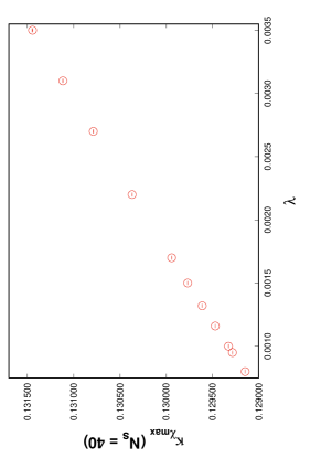
Figure 13: The behavior of ${\kappa_{\chi}}_{\mbox{\scriptsize max}}$ for $N_{s}=40$ as a function of $\lambda$.

VII Discussion and Conclusion

In this work, we study the behavior of the volume average of the Landau gauge-fixed $\Phi^{g}$ and related quantities in $SU(2)-$Higgs theory. The aim of our study is to see if $\Phi^{g}$ behaves like an order parameter for the Higgs transition. We consider $\beta_{g}=8$ as in Aoki:1999fi , and study $\Phi^{g}$ at various values of $\lambda$, from $\lambda=0.00010$ to $\lambda=0.0035$. Our results show that, $\Phi^{g}$ for different $\lambda$ accurately identifies the transitions points ($\kappa_{c}$’s). Across first order transition, $\Phi^{g}$ varies discontinuously, as expected from an order parameter. This is clearly seen at $\lambda=0.00010$ and$\lambda=0.00050$ in agreement with previous study Aoki:1999fi . From $\lambda=0.0008$ onward, we see weakening of transition, with the jump in $\Phi^{g}$ decreasing with $\lambda$. At much higher values of $\lambda$, such as $\lambda=0.00310$ and $\lambda=0.00350$, we see a gradual disappearance of volume dependence signifying a possible crossover. It is interesting to note that a different lattice study Wurtz:2013ova at zero temperature performed at $\beta_{g}=8,\lambda=0.0033,\kappa=0.131$ with a lattice size of $24^{3}\times 48$ has found the physical Higgs mass to be $123(1)$ GeV which is closer to the experimental value.

A significant part our numerical simulations are devoted to study behavior of $\Phi^{g}$ near the end-point. The magnetization, susceptibility, total susceptibility and binder cumulant etc. of $\Phi^{g}$ as functions of $\kappa$ give an impression of an order parameter like behavior at $\lambda_{c}$. The scaling of these quantities for $\nu=0.62997$, $\beta/\nu=0.518$ and $\gamma/\nu=1.964$, shows that the end-point belongs to the $3$d Ising universality class. From the scaling of the Binder cumulant from Fig. 11, we find its value at $(\lambda_{c},\kappa_{c})$ to be consistent with the standard $3$d Ising value of $\sim 0.47$ Ferrenberg:1991 ; Hasenbusch:1998gh .

We mention here that the FSS of $\Phi^{g}$ and its various cumulants suggests that the $\!3$d Ising like behavior seen close to $\lambda=0.00150$ which is within $2\sigma$ of the end-point found in Aoki:1999fi . The FSS of $\Phi^{g}$ seen in Fig. 11 suggests that exactly at the critical point $(\lambda_{c},\kappa_{c})$ $\Phi^{g}$ vanishes. Also the numerical results suggest that for $\lambda<0$ in the Higgs symmetric phase and at $\kappa_{c}$, $\Phi^{g}$ vanishes in the infinite volume limit. This is in contrast to behavior of magnetization in $3$-state Potts model, where the magnetization vanishes in the symmetric phase only in the absence of external field. In the presence of external field, in the symmetric phase at transition point, magnetization increases with external field. This behavior of magnetization $vs$ external field can be be obtained by adding a simple explicit breaking term to Ginzburg-Landau type of mean field free energy. Such an effective description of $\Phi^{g}$ require non-trivial term(s) such that $\Phi^{g}$ is zero in the Higgs symmetric phase at least for $\lambda<\lambda_{c}$.

REFERENCES

References

- (1) V. A. Kuzmin, V. A. Rubakov and M. E. Shaposhnikov, Phys. Lett. B 155, 36 (1985) doi:10.1016/0370-2693(85)91028-7
- (2) V. A. Matveev, V. A. Rubakov, A. N. Tavkhelidze and M. E. Shaposhnikov, Sov. Phys. Usp. 31, 916-939 (1988) doi:10.1070/PU1988v031n10ABEH005633
- (3) V. A. Rubakov and M. E. Shaposhnikov, Usp. Fiz. Nauk 166, 493-537 (1996) doi:10.1070/PU1996v039n05ABEH000145 [arXiv:hep-ph/9603208 [hep-ph]].
- (4) Z. Fodor, KEK-TH-558.
- (5) P. H. Damgaard and U. M. Heller, Nucl. Phys. B 294, 253 (1987) doi:10.1016/0550-3213(87)90582-7
- (6) H. G. Evertz, J. Jersak and K. Kanaya, Nucl. Phys. B 285, 229-252 (1987) doi:10.1016/0550-3213(87)90336-1.
- (7) K. Farakos, K. Kajantie, K. Rummukainen and M. E. Shaposhnikov, Nucl. Phys. B 442, 317-363 (1995) doi:10.1016/0550-3213(95)80129-4 [arXiv:hep-lat/9412091 [hep-lat]].
- (8) K. Kajantie, M. Laine, K. Rummukainen and M. E. Shaposhnikov, Nucl. Phys. B 466, 189-258 (1996) doi:10.1016/0550-3213(96)00052-1 [arXiv:hep-lat/9510020 [hep-lat]].
- (9) K. Rummukainen, M. Tsypin, K. Kajantie, M. Laine and M. E. Shaposhnikov, Nucl. Phys. B 532, 283-314 (1998) doi:10.1016/S0550-3213(98)00494-5 [arXiv:hep-lat/9805013 [hep-lat]].
- (10) M. Gurtler, E. M. Ilgenfritz and A. Schiller, Phys. Rev. D 56, 3888-3895 (1997) doi:10.1103/PhysRevD.56.3888 [arXiv:hep-lat/9704013 [hep-lat]].
- (11) B. Bunk, E. M. Ilgenfritz, J. Kripfganz and A. Schiller, Phys. Lett. B 284, 371-376 (1992) doi:10.1016/0370-2693(92)90447-C
- (12) B. Bunk, E. M. Ilgenfritz, J. Kripfganz and A. Schiller, Nucl. Phys. B 403, 453-474 (1993) doi:10.1016/0550-3213(93)90043-O
- (13) B. Bunk, Nucl. Phys. Proc. Suppl. 42, 566 (1995). doi:10.1016/0920-5632(95)00313-X.
- (14) M. Gurtler, E. M. Ilgenfritz, A. Schiller and C. Strecha, Nucl. Phys. B Proc. Suppl. 63, 563-565 (1998) doi:10.1016/S0920-5632(97)00834-7 [arXiv:hep-lat/9709020 [hep-lat]].
- (15) W. Buchmuller and O. Philipsen, Nucl. Phys. B 443, 47-69 (1995) doi:10.1016/0550-3213(95)00124-B [arXiv:hep-ph/9411334 [hep-ph]].
- (16) K. Kajantie, M. Laine, K. Rummukainen and M. E. Shaposhnikov, Phys. Rev. Lett. 77, 2887-2890 (1996) doi:10.1103/PhysRevLett.77.2887 [arXiv:hep-ph/9605288 [hep-ph]].
- (17) Z. Fodor, J. Hein, K. Jansen, A. Jaster, I. Montvay and F. Csikor, Phys. Lett. B 334, 405-411 (1994) doi:10.1016/0370-2693(94)90706-4 [arXiv:hep-lat/9405021 [hep-lat]].
- (18) Z. Fodor, J. Hein, K. Jansen, A. Jaster and I. Montvay, Nucl. Phys. B 439, 147-186 (1995) doi:10.1016/0550-3213(95)00038-T [arXiv:hep-lat/9409017 [hep-lat]].
- (19) F. Csikor, Z. Fodor, J. Hein and J. Heitger, Phys. Lett. B 357, 156-162 (1995) doi:10.1016/0370-2693(95)00886-P [arXiv:hep-lat/9506029 [hep-lat]].
- (20) F. Karsch, T. Neuhaus, A. Patkos and J. Rank, Nucl. Phys. B 474, 217-234 (1996) doi:10.1016/0550-3213(96)00224-6 [arXiv:hep-lat/9603004 [hep-lat]].
- (21) F. Karsch, T. Neuhaus, A. Patkos and J. Rank, Nucl. Phys. B Proc. Suppl. 53, 623-625 (1997) doi:10.1016/S0920-5632(96)00736-0 [arXiv:hep-lat/9608087 [hep-lat]].
- (22) Y. Aoki, Phys. Rev. D 56, 3860 (1997). doi:10.1103/PhysRevD.56.3860 [hep-lat/9612023].
- (23) Y. Aoki, F. Csikor, Z. Fodor and A. Ukawa, Phys. Rev. D 60, 013001 (1999). doi:10.1103/PhysRevD.60.013001 [hep-lat/9901021].
- (24) C. Bonati, G. Cossu, M. D’Elia and A. Di Giacomo, Nucl. Phys. B 828, 390-403 (2010) doi:10.1016/j.nuclphysb.2009.12.003 [arXiv:0911.1721 [hep-lat]].
- (25) M. D’Onofrio, K. Rummukainen and A. Tranberg, Phys. Rev. Lett. 113, no.14, 141602 (2014) doi:10.1103/PhysRevLett.113.141602 [arXiv:1404.3565 [hep-ph]].
- (26) M. D’Onofrio and K. Rummukainen, Phys. Rev. D 93, no.2, 025003 (2016) doi:10.1103/PhysRevD.93.025003 [arXiv:1508.07161 [hep-ph]].
- (27) M. D’Onofrio, K. Rummukainen and A. Tranberg, PoS LATTICE2012, 055 (2012) doi:10.22323/1.164.0055 [arXiv:1212.3206 [hep-ph]].
- (28) M. Laine, G. Nardini and K. Rummukainen, JCAP 01, 011 (2013) doi:10.1088/1475-7516/2013/01/011 [arXiv:1211.7344 [hep-ph]].
- (29) O. Gould, S. Güyer and K. Rummukainen, [arXiv:2205.07238 [hep-lat]].
- (30) K. Kajantie, Nucl. Phys. B Proc. Suppl. 42, 103-112 (1995) doi:10.1016/0920-5632(95)00192-C [arXiv:hep-lat/9412072 [hep-lat]].
- (31) K. Jansen, Nucl. Phys. B Proc. Suppl. 47, 196-211 (1996) doi:10.1016/0920-5632(96)00045-X [arXiv:hep-lat/9509018 [hep-lat]].
- (32) K. Rummukainen, Nucl. Phys. B Proc. Suppl. 53, 30-42 (1997) doi:10.1016/S0920-5632(96)00597-X [arXiv:hep-lat/9608079 [hep-lat]].
- (33) R. D. Pisarski and F. Wilczek, Phys. Rev. D 29, 338-341 (1984) doi:10.1103/PhysRevD.29.338.
- (34) F. Karsch and S. Stickan, Phys. Lett. B 488, 319-325 (2000) doi:10.1016/S0370-2693(00)00902-3 [arXiv:hep-lat/0007019 [hep-lat]].
- (35) J. L. Alonso, V. Azcoiti, I. Campos, J. C. Ciria, A. Cruz, D. Iniguez, F. Lesmes, C. Piedrafita, A. Rivero and A. Tarancon, et al. Nucl. Phys. B 405, 574-592 (1993) doi:10.1016/0550-3213(93)90560-C [arXiv:hep-lat/9210014 [hep-lat]].
- (36) W. Janke and R. Villanova, Nucl. Phys. B 489, 679-696 (1997) doi:10.1016/S0550-3213(96)00710-9 [arXiv:hep-lat/9612008 [hep-lat]].
- (37) N. B. Wilding, Phys. Rev. E 52, 602-611 (1995) doi:10.1103/PhysRevE.52.602 [arXiv:cond-mat/9503145 [cond-mat]].
- (38) N. B. Wilding and M. Mueller, J. Chem. Phys. 102, 2562 (1995) doi:10.1063/1.468686 [arXiv:cond-mat/9410077 [cond-mat]].
- (39) Nigel B Wilding 1997 J. Phys.: Condens. Matter 9 585.
- (40) J. J. Rehr and N. D. Mermin, Phys. Rev. A 8, 472-480 (1973) doi:10.1103/PhysRevA.8.472.
- (41) K. Kanaya and S. Kaya, Phys. Rev. D 51, 2404-2410 (1995) doi:10.1103/PhysRevD.51.2404 [arXiv:hep-lat/9409001 [hep-lat]].
- (42) D. Toussaint, Phys. Rev. D 55, 362-366 (1997) doi:10.1103/PhysRevD.55.362 [arXiv:hep-lat/9607084 [hep-lat]].
- (43) http://www.physics.utah.edu/~detar/milc/.
- (44) M. Creutz, Phys. Rev. D 21, 2308 (1980). doi:10.1103/PhysRevD.21.2308.
- (45) N. Cabibbo and E. Marinari, Phys. Lett. B 119, 387 (1982). doi:10.1016/0370-2693(82)90696-7.
- (46) C. Whitmer, Phys. Rev. D 29, 306 (1984). doi:10.1103/PhysRevD.29.306.
- (47) S. Aoki et al. [CP-PACS Collaboration], Phys. Rev. D 70, 034503 (2004). doi:10.1103/PhysRevD.70.034503 [hep-lat/0312011].
- (48) M. Wurtz, R. Lewis and T. G. Steele, Phys. Rev. D 79, 074501 (2009) doi:10.1103/PhysRevD.79.074501 [arXiv:0902.1167 [hep-lat]].
- (49) M. Wurtz and R. Lewis, Phys. Rev. D 88, 054510 (2013) doi:10.1103/PhysRevD.88.054510 [arXiv:1307.1492 [hep-lat]].
- (50) Alan M. Ferrenberg and D. P. Landau, Phys. Rev. B 44, 5081, 1991.
- (51) M. Hasenbusch, K. Pinn and S. Vinti, Phys. Rev. B 59, 11471-11483 (1999) doi:10.1103/PhysRevB.59.11471 [arXiv:hep-lat/9806012 [hep-lat]].