Single-shot Kramers–Kronig complex orbital angular momentum spectrum retrieval

Orbital angular momentum (OAM) spectrum diagnosis is a fundamental building block for diverse OAM-based systems. Among others, the simple on-axis interferometric measurement can retrieve the amplitude and phase information of complex OAM spectra in a few shots. Yet, its single-shot retrieval remains illusive, due to the signal-signal beat interference inherent in the measurement. Here, we introduce the concept of Kramers-Kronig (KK) receiver in coherent communications to the OAM domain, enabling rigorous, single-shot OAM spectrum measurement. We explain in detail the working principle and the requirement of the KK method, and then apply the technique to precisely measure various characteristic OAM states. In addition, we discuss the effects of the carrier-to-signal power ratio and the number of sampling points essential for rigorous retrieval, and evaluate the performance on a large set of random OAM spectra and high-dimensional spaces. Single-shot KK interferometry shows enormous potential for characterizing complex OAM states in real-time.

Introduction

Structured light waves with spiral phase fronts carry orbital angular momentum (OAM). Such helical optical beams, either naturally emitted from laser cavities [1] or externally sculpted [2], have recently attracted significant attention and have been widely used in communication, sensing, imaging, as well as classical and quantum information processing [3, 4, 5, 6, 7]. For many of these applications, the ability to diagnose an arbitrary OAM state is essential, so that its complex structure can be unveiled and decomposed into orthogonal OAM basis. Various methods have been explored for the task. Perhaps the most straightforward approach is using vortex phase plates together with a mode filter to obtain the power of each OAM order sequentially [2, 8]. The number of measurements required by this approach however scales fast with the measurement space. Techniques based on the far-field diffraction patterns through certain types of apertures [9] or gratings [10, 11], generally only identify pure OAM orders rather than superimposed states. In that sense, mode sorters are efficient in separating the superposition of OAM modes by mapping different OAM orders into different spatial positions. They have been implemented based on cascaded Mach-Zehnder interferometers with Dove prisms [12], log-polar transformation [13, 14] and its improvement by means of beam-copying [15], or spiral transformation [16] that increase the mode separation. Moreover, multi-plane light conversion is also employed for sorting OAM modes with enhanced functionalities [17, 18, 19]. Yet, mode sorters generally lose the relative phase information among OAM modes, which may be required in many scenarios to unambiguously reconstruct the complex OAM states. For this purpose the interference measurement techniques are appealing for the full OAM field retrieval [20, 21, 22, 23, 24].

Typical OAM interference measurements are performed by recording the interferograms of a complex signal field and a reference OAM mode (or Gaussian beam) with a camera [21, 22, 23]. Since the camera records the light intensity, the complex signal field cannot be directly retrieved from the intensity-only measurement. The measured interferogram intensity, however, consists of not only the desired interference between the signal and reference beams, but also the self-beating of both of them. While the power of the reference is constant across the azimuthal angle, the existence of the signal-signal beat interference (SSBI) complicates the signal retrieval process. Multiple interferograms are thus required to remove the SSBI, by adjusting the power [21, 22] and/or phase [23] of the reference light. Single-shot interferometric measurement has been demonstrated in the context of partially coherent fields, but only for symmetric OAM spectra, while two shots are still needed for generalized spectral shapes [24]. Although the SSBI contribution may be omitted when the reference beam is sufficiently strong [21], rigorous, single-shot retrieval remains elusive for conventional on-axis interferometry.

Notably, the interference measurement of the complex OAM spectrum resembles the detection of complex modulated signals in coherent optical communications, where the reference beam is the counterpart of the local oscillator. Phase-diverse coherent receiver is generally used to retrieve both the amplitude and phase of the modulated signal [25]. In recent years, considerable efforts have been made to reduce the receiver complexity in coherent communication systems, ideally by using only one single-ended photodetector [26, 27, 28, 29, 30, 31]. The Kramers-Kronig (KK) receiver is an effective solution for direct detection of complex-valued signals [28, 29, 30, 31]. In this case, the receiver works in a heterodyne scheme, and requires the frequency of the local oscillator being outside of the signal’s spectrum. When the interfered waveform satisfies the minimum-phase condition [31], the signal can be rigorously reconstructed from the intensity measurement via the famous KK relation. This greatly simplifies the receiver architecture into the straightforward direct detection. In addition, similar KK-based full-field retrieval has also been applied for holographic imaging exploring the space-time duality [32].

In this work, by drawing a close analogy between the time-frequency and azimuth-OAM domains, we extend the KK retrieval concept into the OAM space, for the first time to our knowledge. Such an approach enables the readout of both the amplitude and phase relation of an arbitrary OAM state in a single-shot manner, without increasing the system complexity. We describe in detail the retrieval procedure, which is experimentally validated in a high-dimensional OAM space. In particular, we demonstrate the diagnosis of a number of characteristic OAM states [33, 34, 35, 36], including fractional OAM modes [37] that slightly violates the KK retrieval criteria. The typical parameters essential for a KK receiver [31], i.e., the carrier-to-signal power ratio (CSPR) and the number of sampling points, are discussed in the context of OAM fields. Furthermore, we compare the performances of the proposed KK approach and the conventional Fourier approach for a large set of arbitrary OAM states, where the superiority of the KK approach is clearly shown. The single-shot nature of the KK method may find useful applications for characterizing OAM-based systems in real-time.

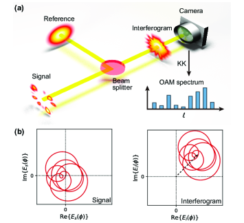
Figure 1: Conceptual setup and the requirement for the Kramers-Kronig (KK) retrieval. (a) The signal field with a complex orbital angular momentum (OAM) spectrum is co-axially combined with a reference Gaussian beam. The intensity of their interferogram is recorded with a camera and is used for the spectrum retrieval. (b) The azimuthal trajectories of the signal (left) and the interferogram (right) in the complex plane. In order to meet the minimum phase condition, the trajectory must not encircle the origin. With the addition of a sufficiently large reference field (denoted by the dashed arrow), the interferogram satisfies the requirement and thus the KK method can rigorously reconstruct the complex signal OAM spectrum.

Results

.1 Principle of operation

A complex OAM field can be described by the controlled superposition in discrete OAM mode basis [33]:

$$E_{s}(\phi)=\sum_{l=l_{0}+1}^{l_{0}+N}a_{l}e^{il\phi+i\theta_{l}},$$ (1)

where $\phi$ is the azimuthal angle, $a_{l}$ and $\theta_{l}$ are the amplitude and phase of the $l$-th OAM mode, respectively. Here we consider the modal decomposition of the OAM field in the interval of $[l_{0}+1,l_{0}+N]$, spanning over a $N$-dimensional space. Without loss of generality we assume $l_{0}=0$ hereafter, as we can always use a phase mask with helical phase $e^{-il_{0}\phi}$ to shift the OAM spectrum entirely above the $0$-th order. In this study the OAM fields are constructed based on perfect vortex modes [38] with identical radial distributions (see Supplementary Note 1), such that we are only interested in field extraction in the azimuthal angle. As shown in Fig. 1(a), the complex signal field is interfered with a reference beam with plane wave front $E_{r}(\phi)=Ae^{i\theta_{r}}$, where $A$ is the amplitude of the reference mode, and $\theta_{r}$ is the relative phase between the reference and signal fields. Similar to the single-sideband modulation for a KK receiver in communications [28], no guard band is needed in between the reference and the signal OAM spectra. Then the interferogram is imaged with a camera and its intensity in the azimuthal angle is proportional to:

$$|E_{i}(\phi)|^{2} =|E_{s}(\phi)+E_{r}(\phi)|^{2}$$ (2)

$$=A^{2}+|E_{s}(\phi)|^{2}+2A\operatorname{Re}\{E_{s}(\phi)e^{-i\theta_{r}}\}$$

$$=A^{2}+|\sum_{l=1}^{N}a_{l}e^{il\phi+i\theta_{l}}|^{2}+2A\sum_{l=1}^{N}a_{l}\cos(l\phi+\theta_{l}-\theta_{r}).$$

The third term in the last equality of Eq. (2) contains all the Fourier coefficients $a_{l}e^{i\theta_{l}}$ required to reconstruct the signal field, apart from scaling and a constant phase shift, while the second term corresponds to the SSBI.

In order to extract the phase information from a single intensity measurement, the amplitude and phase of the interferogram $E_{i}(\phi)$ must be uniquely linked. A way to look at this is using the Z-extension as formulated in Ref. [31]. By replacing the $e^{i\phi}$ in $E_{i}(\phi)$ with a variable $Z$, the interferogram becomes a polynomial function:

$$\mathcal{Z}_{E_{i}}(Z)=Ae^{i\theta_{r}}+\sum_{l=1}^{N}a_{l}e^{i\theta_{l}}Z^{l}=\frac{Ae^{i\theta_{r}}}{\prod_{l=1}^{N}{(-z_{l})}}\prod_{l=1}^{N}{(Z-z_{l})},$$ (3)

where $z_{l}$ ($l=1,2,...,N$) are the roots of $\mathcal{Z}_{E_{i}}(Z)=0$, when $a_{N}\neq 0$. The second equality of Eq. (3) shows that $\mathcal{Z}_{E_{i}}(Z)$ can be equivalently described by its zeros. Since the interferogram is under square-law detection, the zeros of $|E_{i}(\phi)|^{2}$ are found using properties of Z-extension [31]:

$$\mathcal{Z}_{|E_{i}|^{2}}(Z)=\frac{|A|^{2}}{Z^{N}\prod_{l=1}^{N}{(-z_{l})}}\prod_{l=1}^{N}{(Z-z_{l})(Z-\frac{1}{z_{l}^{*}})},$$ (4)

where ^∗ represents the complex conjugate. The zeros of $\mathcal{Z}_{|E_{i}|^{2}}(Z)$ are in $N$ pairs, comprised of the zeros of $\mathcal{Z}_{E_{i}}(Z)$ and the inverse of their complex conjugates. It is noted that replacing the zeros of $\mathcal{Z}_{E_{i}}(Z)$ with their inverse conjugates would not modify the function $\mathcal{Z}_{|E_{i}|^{2}}(Z)$. This implies multiple different interferograms are mapped to the same intensity profile and thus causing ambiguity for the retrieval. If the interferogram is constructed such that all its zeros are outside or on the unit circle, also known as the minimum phase waveform [31], one-to-one mapping between $\mathcal{Z}_{E_{i}}(Z)$ and $\mathcal{Z}_{|E_{i}|^{2}}(Z)$ is established. Evidently, a necessary and sufficient condition to be of a minimum phase waveform is that its trajectory does not encircle the origin of the complex plane [39]. This is visualized in Fig. 1(b). The left panel illustrates the azimuthal trajectory of a general OAM signal field $E_{s}(\phi)$, which does not meet the minimum phase requirement. With a sufficiently large reference field $Ae^{i\theta_{r}}$ (indicated by the dashed arrow), the azimuthal trajectory can be translated to match the minimum phase condition, as shown in the right panel of Fig. 1(b). Consequently, the amplitude and phase of the interferogram $E_{i}(\phi)$ is uniquely related. It is worth mentioning that, for a given signal OAM field, the required reference intensity for the minimum phase condition varies with the relative angle $\theta_{r}$. Nevertheless, since no prior knowledge of the signal field is known, the reference amplitude needs to be greater than the signal’s peak amplitude in the azimuthal angle, i.e., $A>|E_{s}(\phi)|$ for $\phi\in[0,2\pi)$, thereby not encircling the origin. With this we can calculate the minimum CSPR required for rigorous retrieval, which is set by the peak to average power ratio of the signal field.

Once the minimum phase condition is reached, for an interference field $E_{i}(\phi)=|E_{i}(\phi)|e^{i\arg(E_{i}(\phi))}$ ($\arg$ denotes the argument), the logarithm of its amplitude $\log(|E_{i}(\phi)|)$ and phase $\arg(E_{i}(\phi))$ is related by the Hilbert transform [31]:

$$\arg(E_{i}(\phi))=\frac{1}{2\pi}p.v.\int_{0}^{2\pi}\cot{\bigg{(}\frac{\phi-\phi^{\prime}}{2}\bigg{)}}\log(|E_{i}(\phi^{\prime})|)\,d\phi^{\prime},$$ (5)

where $p.v.$ is the principal value. Note that due to the periodic nature of the azimuthal space, the kernel here in the Hilbert transform is in the cotangent form rather than the inverse, and the integration is over one circle [40]. From Eq. (5) we can reconstruct the full-field of the interferogram $E_{i}(\phi)$, and thus also the signal full-field $E_{s}(\phi)$ by removing the constant reference term. Based on the Fourier relation, this equivalently gives the amplitude and phase of the OAM spectrum of $E_{s}(\phi)$.

.2 Experimental KK retrieval procedure

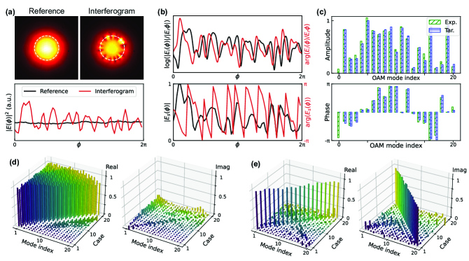
Figure 2: Experimental single-shot KK retrieval. (a)-(c) Retrieval process of an arbitrary OAM spectrum. (a) The intensity images of the reference (top left) and the interferogram (top right) are captured by a camera. By sampling along the dashed circles in the images, their azimuthal distributions are extracted (bottom). (b) The interferogram is then normalized and digitally upsampled, whose phase is extracted from the Hilbert transform of the logarithm of its amplitude (top). From the full-field of the interferogram, the amplitude and phase of the signal is obtained and downsampled to the original sampling points (bottom). (c) Taking the Fourier transform of the signal field derives the normalized amplitude (top) and relative phase relation (bottom) of the OAM spectrum. An accuracy of $97.6\%$ is achieved by comparing the retrieved and the target OAM spectra. (d)-(e) Measured $2$D bar charts of the OAM states for (d) the superpositions of mode indices from $1$ to $n$ ($n=1,2,...,20$) with equal amplitudes and in-phase relations; (e) the superpositions of mode indices $n$ and $21-n$ ($n=1,2,...,20$) with equal amplitudes and a $\pi/2$ phase shift. The average retrieval accuracy in (d) and (e) are $98.9\%$ and $96.0\%$, respectively.

In the experiment, the complex signal OAM fields are synthesized using computer generated holograms and an optical 4-f system [41]. They consist in arbitrary superpositions of ring-shaped OAM modes with topological charges spanning from $1$ to $20$. The OAM fields under test are then co-axially combined with a reference Gaussian beam, and their interferograms are recorded with a camera. The detailed experimental setup is described in the Supplementary Note 1. To satisfy the minimum phase condition, we tune the reference light power slightly above the power threshold set by the minimum required CSPR. Thanks to the signal preparation method we used [41], the experimental and minimum required CSPR difference is kept constant ($\sim 1\leavevmode\nobreak\ {\rm dB}$) for different measurement instances (see Supplementary Note 2). In the following, we demonstrate the KK retrieval procedure on a random complex OAM spectrum as an example. The top panel of Fig. 2(a) shows the measured camera images of the reference and the interference beams. Their azimuthal intensity distributions are extracted by sampling around the interfered regions (indicated by the dashed circles), and unwrapped as shown in the bottom panel of Fig. 2(a). It can be seen that the measured reference $|E_{r}(\phi)|^{2}$ shows small intensity fluctuations in the azimuth direction. Such a reference intensity pattern is unchanged while characterizing different signal OAM fields, so only their interferogram $|E_{i}(\phi)|^{2}$ needs to be measured each time, suggesting that the retrieval process is a single-shot.

Similar to the KK full-field retrieval in space and time [28, 32], digital upsampling may also be required in our case, if the number of physical sampling points is not sufficiently large to cover the spectrum expended by the logarithmic operation [31]. The effect of upsampling is discussed in Supplementary Note 3. Throughout the paper we take $71$ azimuthal sampling points in the experiment, and then we digitally upsample the normalized interferogram $|E_{i}(\phi)|^{2}/|E_{r}(\phi)|^{2}$ by $11$-times for the subsequent processing. The top panel of the Fig. 2(b) shows the logarithm of the upsampled interferogram $\log(|E_{i}(\phi)|/|E_{r}(\phi)|)$ as well as its Hilbert transform $\arg(E_{i}(\phi)/E_{r}(\phi))$. Instead of taking the convolution as defined in Eq. (5), the actual implementation of the Hilbert transform is realized in the spectral domain using the fast Fourier transform and the sign function [28]. The full-field of the interferogram $E_{i}(\phi)/E_{r}(\phi)$ is thus derived, from which the full signal field can be easily calculated by $E_{s}(\phi)\approx|E_{r}(\phi)|(E_{i}(\phi)/E_{r}(\phi)-1)$. Here we omit the negligible phase non-uniformity of the experimental reference beam. The retrieved signal field is then downsampled, whose normalized amplitude $|E_{s}(\phi)|$ and phase $\arg(E_{s}(\phi))$ are plotted in the bottom panel of Fig. 2(b). Finally, the complex signal OAM spectrum is retrieved by taking the Fourier transform of $E_{s}(\phi)$. Figure 2(c) illustrates the retrieved amplitude (top) and phase (bottom) profile of the OAM spectrum and are compared to the ground truth. It can be seen that they are in excellent agreement. To quantitatively assess the performance of the KK retrieval, we introduce the following metric based on the overlap integral of the target and the retrieved OAM spectra:

$$\eta=\frac{|\sum_{-\infty}^{\infty}a_{l}a_{l}^{\prime}e^{i\theta_{l}-i\theta_{l}^{\prime}}|^{2}}{(\sum_{-\infty}^{\infty}|a_{l}|^{2})(\sum_{-\infty}^{\infty}|a_{l}^{\prime}|^{2})},$$ (6)

where $a_{l}^{\prime}$ and $\theta_{l}^{\prime}$ are the amplitude and phase of the $l$-th order OAM mode of the retrieved OAM spectrum, respectively. In Fig. 2(c), the retrieval accuracy $\eta$ is found to be $97.6\%$.

To further test the validity of the proposed method, we apply the KK retrieval to diagnose a series of OAM spectra shown in Figs. 2(d) and 2(e). The first scenario is the rectangular OAM spectra $E_{s}(\phi)=\sum_{l=1}^{n}e^{il\phi}$ of different widths ($n=1,2,...,20$), where the constituent OAM modes are of equal amplitudes and in-phase relations. Figure 2(d) shows the real and imaginary parts of the measured OAM spectra for these cases in a complex $2$D bar chart. As expected, the retrieved OAM spectra are approximately of rectangular shapes, and are mainly populated in the real part of the bar chart due to their in-phase features. An average accuracy of $98.9\%$ is achieved for these measurements. For the second scenario, the OAM spectra are structured by $E_{s}(\phi)=e^{in\phi}+ie^{i(21-n)\phi}$, where $n=1,2,...,20$. In this case, the bar chart should be diagonal in its real part while anti-diagonal in its imaginary part. This is clearly observed in the measurements shown in Fig. 2(e), with an average retrieval accuracy reaching $96.0\%$.

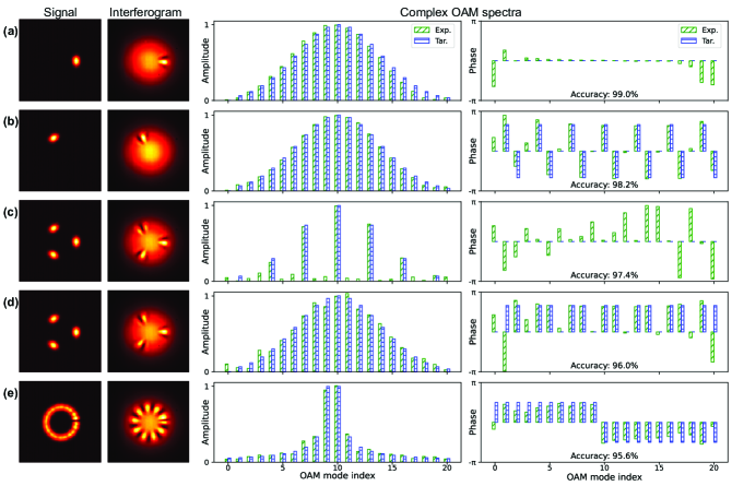
Figure 3: Measurements of complex OAM spectra. Left: the measured intensity images of the signal and the interferogram; Right: the normalized amplitude and relative phase of the target and experimentally retrieved OAM spectrum. (a)-(d) Gaussian-shaped OAM spectra centered at $10$-th order with versatile OAM mode spacings and relative phase relations. (a) In-phase OAM spectrum with a mode spacing of $1$. (b) Linear-phase OAM spectrum with a phase slope of $2\pi/3$ and a mode spacing of $1$. (c) In-phase OAM spectrum with a mode spacing of $3$. (d) OAM spectrum with periodic Talbot phase $[0,2\pi/3,2\pi/3]$ and a mode spacing of $1$. (e) Fractional OAM mode with a topological charge of $9.5$. The retrieval accuracy is also indicated for each case.

.3 Measurement of characteristic OAM states

The single-shot KK full-field retrieval allows for the simple characterization of complex OAM states. In the following, we study various characteristic OAM spectra displayed in Fig. 3. Figure 3(a) demonstrates the measurement of a signal field with a Gaussian-shaped, in-phase OAM spectrum centered at $10$-th order, i.e., $E_{s}(\phi)=\sum_{l=1}^{20}e^{-\frac{(l-10)^{2}}{30}}e^{il\phi}$, which corresponds to a bright petal horizontally aligned in the azimuthal angle [33]. From only a single interferogram we can reconstruct the signal’s OAM spectrum well matching the ground truth. Note that all the measured images of the signal beams in Fig. 3 are displayed only for the illustration purpose, and are not used for their OAM spectra retrieval. Figure 3(b) shows the condition for the same petal field as in Fig. 3(a) except being rotated by $2\pi/3$ counterclockwise. A linear phase ramp is thus imparted to the OAM spectrum due to the rotation, with a phase slope of $2\pi/3$. This feature is well captured by the KK approach in a single-shot fashion, simplifying the previously used schemes like the sequential weak and strong measurements [34] or the phase-shifting holograms [42].

In addition, it is known that increasing the mode spacing in the OAM spectrum will lead to the multiplication of petals in the azimuthal angle [33]. This is shown in Fig. 3(c), where a $3$-petal field under test is constructed from in-phase OAM modes with an order spacing of $3$ and the same envelope as in Figs. 3(a) and 3(b). The interferogram could accurately retrieve its equidistant OAM structure as well as its in-phase relation. Notice that the large phase error in Fig. 3(c) is only associated with void OAM modes or at small modal amplitudes. Furthermore, we investigate the complex OAM spectrum of the petal field in Fig. 3(c) being subjected to phase modulation. Specifically, when the $3$ petals are modulated with the Talbot phase sequence of $[0,-2\pi/3,-2\pi/3]$, the initial OAM spectrum is self-imaged to create new OAM modes, meanwhile preserving its overall envelope [36]. The measurement results are shown in Fig. 3(d). Although the signal intensity patterns in Figs. 3(c) and 3(d) are identical, the phenomenon of the OAM spectral self-imaging is clearly observed from the KK retrieval. More interestingly, the approach also provides a direct phase measurement of all the OAM modes. It can be seen that the relative phases of OAM self-images again follow the Talbot relation of $[0,2\pi/3,2\pi/3]$, apart from a constant phase (subtracted thus not shown in Fig. 3(d) for better representability). Notably, such a phase structure of Talbot self-images has only been recently determined in space [43] and time [44], while here we measure it for the first time in the OAM basis.

We also use the KK method to characterize the complex spectra of fractional OAM modes. A fractional OAM order can be viewed as the weighted superposition of integer OAM modes [45]. In Fig. 3(e), we show the measurement of the fractional OAM field with a topological charge of $9.5$, i.e., $E_{s}(\phi)=e^{i9.5\phi}$. The field intrinsically exhibits around $1\%$ power leakage to the negative OAM orders, thus not rigorously satisfying the single-sideband requirement. Nevertheless, since the leakage is small, the KK retrieval still works effectively with the accuracy of $95.6\%$. We can see that the fractional OAM field in Fig. 3(e) is mainly composed of the $9$-th and $10$-th OAM modes, together with the other OAM orders slowly decaying when moving away from the center modes. Moreover, we are able to identify the phase relation of its constituent OAM modes, which is rarely explored for the fractional OAM states. It is found that the orders at left and right parts of the fractional OAM spectrum are approximately out-of-phase. The phase deviation between the measured and theoretical fractional OAM spectra may come in part from the finite sampling in the azimuthal angle.

.4 Effect of CSPR levels

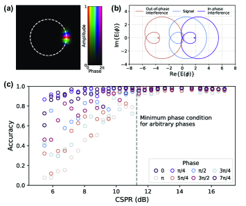
Figure 4: KK retrieval at different carrier-to-signal power ratio (CSPR) levels. (a) The complex amplitude field of the signal used for the study [same as the signal field in Fig. 3(a)]. (b) The azimuthal trajectories of the signal field and interferograms with in-phase and out-of-phase addition of the reference field. The trajectories of interferograms are exactly at the limit of the minimum phase condition, which correspond to the minimum required CSPRs of $5.1\leavevmode\nobreak\ {\rm dB}$ (in-phase) and $11.3\leavevmode\nobreak\ {\rm dB}$ (out-of-phase), respectively. (c) The accuracy of the KK retrieval at different CSPR levels and varying phases between the signal and reference fields. Below the CSPR threshold for arbitrary phases ($11.3\leavevmode\nobreak\ {\rm dB}$, indicated by the dashed line), the retrieval performance varies with the phase; while above, the retrieval accuracy is approximately close to the unity for all the phases.

Figure 4 shows the KK retrieval performance at different CSPR levels. As an example, the same OAM state in Fig. 3(a) is used as the signal field for the study, whose complex amplitude field is displayed in Fig. 4(a). From this we can plot in Fig. 4(b) the trajectory of its azimuthal distribution in the complex plane. As mentioned previously, to guarantee the rigorous KK retrieval, the trajectory of the signal field after interfering with the reference light must not encircle the origin of the complex plane. The minimum required reference intensity for such a criterion is highly dependant on the relative angle between the reference and the signal fields. In Fig. 4(b), the minimum required CSPR varies in a range between $5.1\leavevmode\nobreak\ {\rm dB}$ and $11.3\leavevmode\nobreak\ {\rm dB}$, where the lower and upper bounds correspond to the reference field being added in-phase ($\theta_{r}=0$) and out-of-phase ($\theta_{r}=\pi$) with the signal field, respectively. The minimum required CSPR value valid for all these relative angles is thus set by the upper bound, i.e., $11.3\leavevmode\nobreak\ {\rm dB}$.

Figure 4(c) presents the experimental results for the retrieval accuracy at different CSPR levels and various relative phases between the signal and reference fields. In the experiment, the control of the CSPR and their relative phase are realized via the computer generated holograms. The phases shown in Fig. 4(c) are varied in steps of $\pi/4$. We emphasize here that they do not correspond to the actual $\theta_{r}$, but are offset from a constant unknown phase due to experimental constraints. In Fig. 4(c), when the experimental CSPR is well below the $11.3\leavevmode\nobreak\ {\rm dB}$ threshold (marked by the dashed line), the retrieval performance changes significantly with the phase, although for some angles the retrieval accuracy are acceptable. Once the CSPR exceeds the threshold, decent retrieval is achieved for arbitrary relative phases between the reference and signal fields. The experimental results in Fig. 4(c) are in accordance with the theoretical analysis carried out above.

.5 Performance evaluation

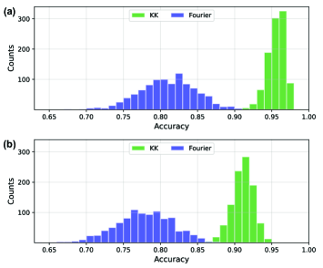
Figure 5: Performance evaluation of the KK retrieval on random OAM spectra. (a)-(b) Histograms of the retrieval accuracy of the KK method and the conventional Fourier method, measured on $1000$ OAM spectra with random complex mode coefficients. (a) For an OAM measurement range from $1$ to $20$, the average and standard deviation of the KK retrieval accuracy are $95.6\%$ and $1.2\%$, respectively. (b) For an OAM measurement range from $1$ to 30, the average and standard deviation of the KK retrieval accuracy are $91.1\%$ and $1.4\%$, respectively. The KK method shows superiority over the Fourier method in both cases.

In this part, we evaluate the performance of the KK retrieval on a large set of OAM spectra generated with random complex mode coefficients. As in the previous measurements, the difference between the experimental and minimum required CSPRs is automatically maintained around $1\leavevmode\nobreak\ {\rm dB}$, which is experimentally confirmed in Supplementary Note 2 for $100$ random OAM spectra. Figure 5(a) shows the histogram of the KK retrieval accuracy for $1000$ spectrum samples on the same dimensional space as before. An average retrieval accuracy of $95.6\%$ is obtained with a standard deviation of $1.2\%$. The performance of the KK retrieval is also compared with the conventional Fourier method, computed by the Fourier transform disregarding the SSBI in Eq. (2). A clear advantage of using the KK method can be seen in Fig. 5(a). Next, we further push the measurement dimensionality up to $30$-th OAM order, while keeping the azimuthal sampling points and the digital upsampling unchanged. Figure 5(b) shows the corresponding experimental results. The average KK retrieval accuracy in this case still reaches $91.1\%$ with a standard deviation of $1.4\%$, outperforming the conventional Fourier method by a large margin. Although the performance of the Fourier method may be improved by increasing the reference power, keeping relatively low CSPR values is favored to avoid large DC components in detection and thus maximally utilize the dynamic range of the camera.

Discussion

The experimental setup used in this work is a conventional on-axis interferometer equivalent to the configurations in Refs. [21, 22, 23]. However, contrary to all the past demonstrations that require a few shots to diagnose a complex OAM spectrum, our method provides single-shot retrieval mediated by the famous KK relation. This greatly accelerate the measurement as it bypasses the need to adjust the amplitude and/or phase of the reference when characterizing each superimposed state [21, 22, 23]. In our system, the speed of the measurement is defined by the frame rate of the camera. Since in this study we are dealing with only the azimuthal field distribution, the detection can be seamlessly connected to the rotational Doppler effect [46]. In this scenario, the camera is replaced by a fast photodetector with a spinning phase mask performing the azimuth-to-time mapping [21].

To sum up this work, we propose and experimentally demonstrate a high-dimensional OAM analyzer that can measure complex OAM states in one single shot. The idea is inspired by the KK receiver in optical communications, while here we introduce the same concept to the OAM spectrum analysis. As demonstrated here, this enables the simple characterization of a wide variety of complex OAM spectra, and can be extended to the measurements of multiple concentric OAM states as well as, in principle, the superposition of Laguerre-Gaussian modes. The proposed single-shot KK interferometry can be readily employed for state measurements in OAM-based information processing, sensing, and communication systems. This work also implies the general duality between azimuth-OAM and time-frequency, suggesting that their processing techniques may be borrowed interchangeably.

Funding: National Key Research and Development Program of China (2018YFB1801803, 2019YFA0706302); Basic and Applied Basic Research Foundation of Guangdong Province (2021B1515020093, 2021B1515120057); Local Innovative and Research Teams Project of Guangdong Pearl River Talents Program (2017BT01X121); Swiss National Science Foundation (P2ELP2$\_$199825).

Data Availability Statement: The data and code that support the plots within this paper and other findings of this study are available from the corresponding authors upon reasonable request.

References

- Naidoo et al. [2016] D. Naidoo, F. S. Roux, A. Dudley, I. Litvin, B. Piccirillo, L. Marrucci, and A. Forbes, Nature Photonics 10, 327 (2016).
- Forbes et al. [2016] A. Forbes, A. Dudley, and M. McLaren, Advances in Optics and Photonics 8, 200 (2016).
- Willner et al. [2015] A. E. Willner, H. Huang, Y. Yan, Y. Ren, N. Ahmed, G. Xie, C. Bao, L. Li, Y. Cao, Z. Zhao, et al., Advances in Optics and Photonics 7, 66 (2015).
- Rubinsztein-Dunlop et al. [2016] H. Rubinsztein-Dunlop, A. Forbes, M. V. Berry, M. R. Dennis, D. L. Andrews, M. Mansuripur, C. Denz, C. Alpmann, P. Banzer, T. Bauer, et al., Journal of Optics 19, 013001 (2016).
- Padgett [2017] M. J. Padgett, Optics Express 25, 11265 (2017).
- Erhard et al. [2018] M. Erhard, R. Fickler, M. Krenn, and A. Zeilinger, Light: Science & Applications 7, 17146 (2018).
- Shen et al. [2019] Y. Shen, X. Wang, Z. Xie, C. Min, X. Fu, Q. Liu, M. Gong, and X. Yuan, Light: Science & Applications 8, 1 (2019).
- Schulze et al. [2013] C. Schulze, A. Dudley, D. Flamm, M. Duparre, and A. Forbes, New Journal of Physics 15, 073025 (2013).
- Hickmann et al. [2010] J. Hickmann, E. Fonseca, W. Soares, and S. Chávez-Cerda, Physical Review Letters 105, 053904 (2010).
- Dai et al. [2015] K. Dai, C. Gao, L. Zhong, Q. Na, and Q. Wang, Optics Letters 40, 562 (2015).
- Zheng and Wang [2017] S. Zheng and J. Wang, Scientific Reports 7, 1 (2017).
- Leach et al. [2002] J. Leach, M. J. Padgett, S. M. Barnett, S. Franke-Arnold, and J. Courtial, Physical Review Letters 88, 257901 (2002).
- Berkhout et al. [2010] G. C. Berkhout, M. P. Lavery, J. Courtial, M. W. Beijersbergen, and M. J. Padgett, Physical Review Letters 105, 153601 (2010).
- Lavery et al. [2012] M. P. Lavery, D. J. Robertson, G. C. Berkhout, G. D. Love, M. J. Padgett, and J. Courtial, Optics Express 20, 2110 (2012).
- Mirhosseini et al. [2013] M. Mirhosseini, M. Malik, Z. Shi, and R. W. Boyd, Nature Communications 4, 1 (2013).
- Wen et al. [2018] Y. Wen, I. Chremmos, Y. Chen, J. Zhu, Y. Zhang, and S. Yu, Physical Review Letters 120, 193904 (2018).
- Labroille et al. [2014] G. Labroille, B. Denolle, P. Jian, P. Genevaux, N. Treps, and J.-F. Morizur, Optics Express 22, 15599 (2014).
- Fontaine et al. [2019] N. K. Fontaine, R. Ryf, H. Chen, D. T. Neilson, K. Kim, and J. Carpenter, Nature Communications 10, 1 (2019).
- Zhang et al. [2020] Y. Zhang, H. Wen, A. Fardoost, S. Fan, N. K. Fontaine, H. Chen, P. L. Likamwa, and G. Li, arXiv preprint arXiv:2010.04859 (2020).
- Huang et al. [2013] H. Huang, Y. Ren, Y. Yan, N. Ahmed, Y. Yue, A. Bozovich, B. I. Erkmen, K. Birnbaum, S. Dolinar, M. Tur, et al., Optics Letters 38, 2348 (2013).
- Zhou et al. [2017] H.-L. Zhou, D.-Z. Fu, J.-J. Dong, P. Zhang, D.-X. Chen, X.-L. Cai, F.-L. Li, and X.-L. Zhang, Light: Science & Applications 6, e16251 (2017).
- D’Errico et al. [2017] A. D’Errico, R. D’Amelio, B. Piccirillo, F. Cardano, and L. Marrucci, Optica 4, 1350 (2017).
- Fu et al. [2020] S. Fu, Y. Zhai, J. Zhang, X. Liu, R. Song, H. Zhou, and C. Gao, PhotoniX 1, 1 (2020).
- Kulkarni et al. [2017] G. Kulkarni, R. Sahu, O. S. Magaña-Loaiza, R. W. Boyd, and A. K. Jha, Nature Communications 8, 1 (2017).
- Ip et al. [2008] E. Ip, A. P. T. Lau, D. J. Barros, and J. M. Kahn, Optics Express 16, 753 (2008).
- Peng et al. [2009] W.-R. Peng, X. Wu, K.-M. Feng, V. R. Arbab, B. Shamee, J.-Y. Yang, L. C. Christen, A. E. Willner, and S. Chi, Optics Express 17, 9099 (2009).
- Randel et al. [2015] S. Randel, D. Pilori, S. Chandrasekhar, G. Raybon, and P. Winzer, in 2015 European Conference on Optical Communication (ECOC) (IEEE, 2015) pp. 1–3.
- Mecozzi et al. [2016] A. Mecozzi, C. Antonelli, and M. Shtaif, Optica 3, 1220 (2016).
- Li et al. [2017] Z. Li, M. S. Erkılınç, K. Shi, E. Sillekens, L. Galdino, B. C. Thomsen, P. Bayvel, and R. I. Killey, Journal of Lightwave Technology 35, 1887 (2017).
- Bo and Kim [2018] T. Bo and H. Kim, Optics Express 26, 13810 (2018).
- Mecozzi et al. [2019] A. Mecozzi, C. Antonelli, and M. Shtaif, Advances in Optics and Photonics 11, 480 (2019).
- Baek et al. [2019] Y. Baek, K. Lee, S. Shin, and Y. Park, Optica 6, 45 (2019).
- Xie et al. [2017a] G. Xie, C. Liu, L. Li, Y. Ren, Z. Zhao, Y. Yan, N. Ahmed, Z. Wang, A. J. Willner, C. Bao, et al., Optics Letters 42, 991 (2017a).
- Malik et al. [2014] M. Malik, M. Mirhosseini, M. P. Lavery, J. Leach, M. J. Padgett, and R. W. Boyd, Nature Communications 5, 1 (2014).
- Hu et al. [2018] J. Hu, C.-S. Brès, and C.-B. Huang, Optics Letters 43, 4033 (2018).
- Lin et al. [2021] Z. Lin, J. Hu, Y. Chen, S. Yu, and C.-S. Brès, APL Photonics 6, 111302 (2021).
- Götte et al. [2008] J. B. Götte, K. O’Holleran, D. Preece, F. Flossmann, S. Franke-Arnold, S. M. Barnett, and M. J. Padgett, Optics Express 16, 993 (2008).
- Vaity and Rusch [2015] P. Vaity and L. Rusch, Optics Letters 40, 597 (2015).
- Mecozzi [2016] A. Mecozzi, arXiv preprint arXiv:1606.04861 (2016).
- Cizek [1970] V. Cizek, IEEE Transactions on Audio and Electroacoustics 18, 340 (1970).
- Arrizón et al. [2007] V. Arrizón, U. Ruiz, R. Carrada, and L. A. González, JOSA A 24, 3500 (2007).
- Xie et al. [2017b] G. Xie, H. Song, Z. Zhao, G. Milione, Y. Ren, C. Liu, R. Zhang, C. Bao, L. Li, Z. Wang, et al., Optics Letters 42, 4482 (2017b).
- De Chatellus et al. [2015] H. G. De Chatellus, E. Lacot, O. Hugon, O. Jacquin, N. Khebbache, and J. Azaña, JOSA A 32, 1132 (2015).
- Clement et al. [2020] J. Clement, H. G. de Chatellus, and C. R. Fernández-Pousa, Optics Express 28, 12977 (2020).
- Zhang et al. [2022] H. Zhang, J. Zeng, X. Lu, Z. Wang, C. Zhao, and Y. Cai, Nanophotonics 11, 241 (2022).
- Courtial et al. [1998] J. Courtial, K. Dholakia, D. Robertson, L. Allen, and M. Padgett, Physical Review Letters 80, 3217 (1998).