Enhanced Deep Animation Video Interpolation

Abstract

Existing learning-based frame interpolation algorithms extract consecutive frames from high-speed natural videos to train the model. Compared to natural videos, cartoon videos are usually in a low frame rate. Besides, the motion between consecutive cartoon frames is typically nonlinear, which breaks the linear motion assumption of interpolation algorithms. Thus, it is unsuitable for generating a training set directly from cartoon videos. For better adapting frame interpolation algorithms from nature video to animation video, we present AutoFI, a simple and effective method to automatically render training data for deep animation video interpolation. AutoFI takes a layered architecture to render synthetic data, which ensures the assumption of linear motion. Experimental results show that AutoFI performs favorably in training both DAIN and ANIN. However, most frame interpolation algorithms will still fail in error-prone areas, such as fast motion or large occlusion. Besides AutoFI, we also propose a plug-and-play sketch-based post-processing module, named SktFI, to refine the final results using user-provided sketches manually. With AutoFI and SktFI, the interpolated animation frames show high perceptual quality.

Index Terms—  animation frame interpolation, nonlinear motion, dataset, neural network

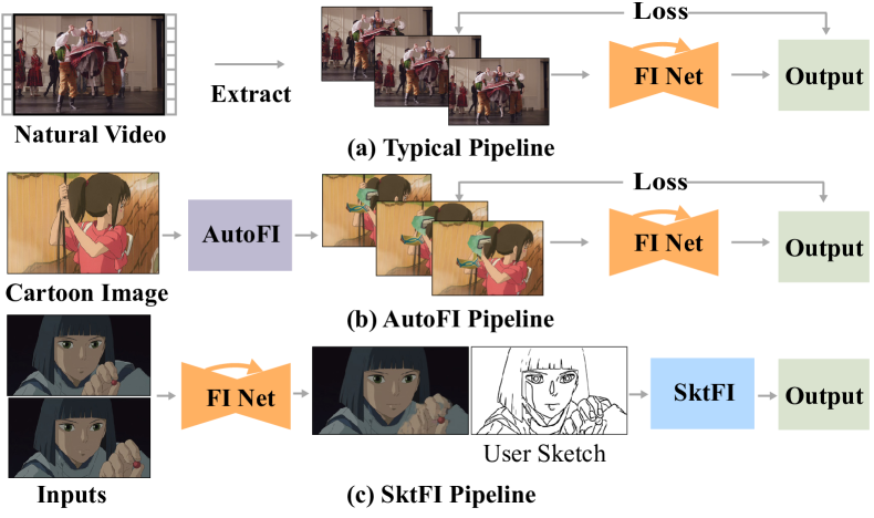
Fig. 1: Pipelines for video frame interpolation. A typical pipeline in (a) extracts three consecutive frames from a natural video. The first and the third frames are inputs for the interpolation network, and the middle one is used as the ground-truth frame. AutoFI in (b) uses a single background cartoon image and masked layers to synthesize triplet frames with linear motions. SktFI in (c) utilizes user-provided sketch to rectify error-prone areas in frame interpolation algorithms.

1 Introduction

Learning-based frame interpolation algorithms boot numerous applications, such as slow motion generation [1], neural view rendering [2], frame rate up-conversion [3, 4, 5, 6]. Datasets are the critical driving force for training a frame interpolation algorithm. Most state-of-the-art frame interpolation algorithms use extracted consecutive frames from high-speed natural videos for training, such as dataset Vimeo90K [7], Adobe240 [8]. Compared to natural videos, cartoon videos usually have low frame rates. In the animation industry, drawing an in-between frame cost complex and enormous labor. Producers usually replicate one frame two or three times to save cost. Besides, unlike nature videos, the motion between consecutive cartoon frames is typically nonlinear, which breaks the linear motion assumption for frame interpolation [3, 1]. Thus, it is unsuitable to directly generate a training set from cartoon videos to adapt frame interpolation algorithms from nature video to animation video.

ANIN [9] is the most related work that considers animation video frame interpolation using a deep neural network. ANIN proposes Segment-Guided Matching to address the cartoon frame alignment problem. Their training set is manually selected from cartoon frames that appear to move linearly. However, manual selection severely limits the scalability of training and can not avoid the non-linearity, which misleads the frame synthesis network, resulting in blurry interpolated frames, as shown in Figure 7.

In this paper, we first present AutoFI (see Figure 1(b)), a simple and effective method to Automatically render training data for deep animation video Frame Interpolation. AutoFI takes a layered architecture to render three consecutive cartoon frames using a single background image and masked layers. AutoFI ensures the basic assumption of linear motion, the interpolation network trained using AutoFI (e.g., DAIN [3] and ANIN [9]) presents clear and high-quality content. However, most frame interpolation algorithms will still fail at error-prone areas, such as fast motion or large occlusion. Besides AutoFI, we also propose a plug-and-play Sketch-based Frame Interpolation module, named SktFI (see Figure 1(c)), to manually refine the final results using user-provided sketches. With AutoFI and SktFI, the interpolated animation frames show high perceptual quality. In this paper, we have the following contributions: 1) we first present AutoFI, an effective method for arbitrary rendering training data for animation in-between; 2) we introduce SktFI, a practical post-processing module to rectify error-prone areas in frame interpolation; 3) Numerical and visual results demonstrate the effectiveness of our method.

2 Methodology

2.1 AutoFI Pipeline

Given two animation frames $\mathbf{I}_{1}$ and $\mathbf{I}_{3}$, the goal of frame interpolation is to synthesize an intermediate frame $\hat{\mathbf{I}}_{2}$. The training set for learning-based frame interpolation algorithms typically contains three frames $\mathbf{I}_{1}$, $\mathbf{I}_{2}$ and $\mathbf{I}_{3}$. $\mathbf{I}_{1}$ and $\mathbf{I}_{3}$ are used as input and $\mathbf{I}_{2}$ is used as the ground-truth frame for supervised learning. AutoFI aims to enhance the perceptual quality of interpolated frames by generating a training set on animation videos to reduce domain bias and then training frame interpolation. AutoFI takes a layered approach [10, 11, 12] to synthesize consecutive frames $\mathbf{I}_{1}$, $\mathbf{I}_{2}$ and $\mathbf{I}_{3}$ by using one background frame and several masked layered contents.

Here, we introduce the AutoFI pipeline, as shown in Figure 2. We first construct an image dataset $\mathcal{S}$ by independently extracting images from an animation video, such as Spirited Away. Notice that the image dataset $\mathcal{S}$ does not need consecutive video frames. For the background layer (i.e., the first layer with $k=1$), we randomly select one image $\mathbf{I}_{1}^{k=1}$ from $\mathcal{S}$, as shown in Figure 2. For upper layers with $k\in[2,K]$, we also randomly select one image from the image dataset $\mathcal{S}$, defined as $\mathbf{I}_{1}^{k}$, where $k\in[2,K]$. Besides, we generate binary mask $\mathbf{M}_{1}^{k}$ for upper layers. The mask is generated using random polygons, as shown in Figure 3.

For each layer, we also generate random per-pixel motion field (i.e., optical flow) between consecutive frames using homography transformation, defined by $\mathbf{F}_{1\rightarrow 2}^{k}$ and $\mathbf{F}_{1\rightarrow 3}^{k}$. Notice that under the linear motion assumption, we set:

$$\mathbf{F}_{1\rightarrow 3}^{k}=2\cdot\mathbf{F}_{1\rightarrow 2}^{k}.$$ (1)

The optical flows are used to warp $\mathbf{I}_{1}^{k}$ to the time index $n$:

$$\mathbf{I}_{n}^{k} =\mathcal{W}(\mathbf{I}_{1}^{k},\mathbf{F}_{1\rightarrow n}^{k}),\quad\quad k\in[1,K],n\in\{2,3\},$$ (2)

$$\mathbf{M}_{n}^{k} =\mathcal{W}(\mathbf{M}_{1}^{k},\mathbf{F}_{1\rightarrow n}^{k}),\quad k\in[1,K],n\in\{2,3\},$$ (3)

where $\mathcal{W}(\cdot)$ is the forward-warping function, which we adopt SoftmaxSplat[2] with the average splatting mode.

We then conduct an iterative layered approach to construct the final frame by iterating from $k=1$ to $k=K$:

$$\mathbf{I}_{n} :=(\mathbf{1}-\mathbf{M}_{n}^{k})\cdot\mathbf{I}_{n}+\mathbf{M}_{n}^{k}\cdot\mathbf{I}_{n}^{k},k\in[1,K],n\in[1,3],$$ (4)

where the initial values for the background layer (i.e., $k=1$) are set $\mathbf{I}_{1}=\mathbf{0}$ and $\mathbf{M}_{n}^{1}=\mathbf{1}$. Notice that we could also obtain ground-truth optical flows by:

$$\mathbf{F}_{1\rightarrow n} :=(\mathbf{1}-\mathbf{M}_{n}^{k})\cdot\mathbf{F}_{1\rightarrow n}+\mathbf{M}_{n}^{k}\cdot\mathbf{F}_{1\rightarrow n}^{k},$$ (5)

where $k\in[1,K],n\in[2,3]$. However, this paper does not utilize the flows for training frame interpolation models. The ground-truth flows could facilitate related optical flow estimation algorithms for future research [13, 14].

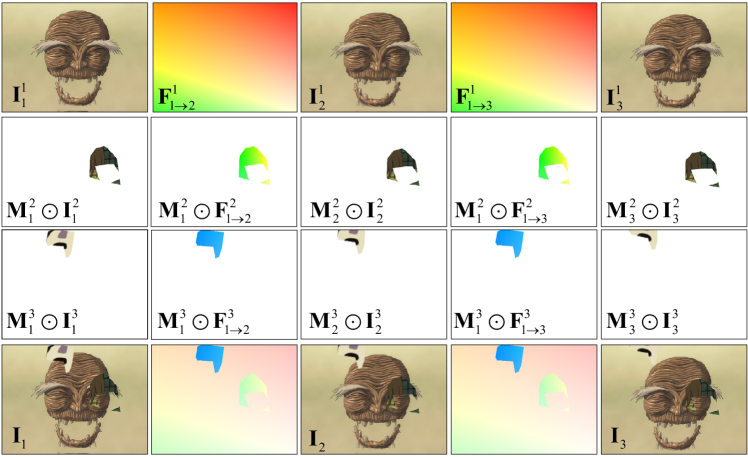
Fig. 2: AutoFI pipeline. Using $K=2$ as an example.

Layer Mask.

We generate random convex polygons [12] as binary masks for the upper layers with $k\in[2,K]$ to simulation object movements. The synthesized polygons have a random number of sides, and we randomly make the hole by nesting a small polygon into it, as shown in Figure 3. Similar to the previous work[12], we apply a Gaussian Blur filter on both the layer masks and masked objects. The standard deviation $\delta$ of Gaussian blur is calculated by evaluating the average flow magnitude over the mask:

$$\delta=\text{log}\big{(}\frac{\text{sum}(||\mathbf{M}_{n}^{k}\cdot\mathbf{F}_{1\rightarrow n}^{k}||)}{\text{sum}(||\mathbf{M}_{n}^{k}||)\cdot\alpha}\big{)},$$ (6)

where scaling factor $\alpha$ is set as $0.1$ empirically.

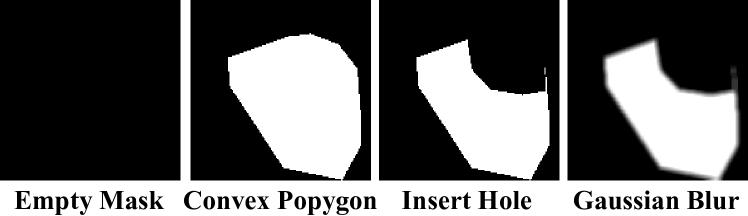
Fig. 3: Illustration of layer masks with random polygons.

Motion Field.

We use random homography transformation to synthesize optical flows (see Equation (1)), which combines several types of motion, including scale, rotation, translation, and perspective motion. We first generate a random homography matrix, denoted by $\mathbf{H}$. We then compute the transformed pixel location by:

$$\mathbf{y}(p)=\mathbf{H}\cdot\mathbf{x}(p),$$ (7)

where $\mathbf{x}(p)$ is the pixel location of pixel $p$ and $\mathbf{y}(p)$ refers to the transformed location. We compute the motion vector by:

$$\mathbf{f}_{x\rightarrow y}(p)=\mathbf{y}(p)-\mathbf{x}(p).$$ (8)

The optical flow field $\mathbf{F}_{1\rightarrow n}$ is a set collecting all pixels $p$, defined by $\mathbf{F}_{1\rightarrow n}=\{\mathbf{f}_{1\rightarrow n}(p)~{}|~{}\forall p\}$. Notice that here we drop superscript $k$ for $\mathbf{F}_{1\rightarrow n}^{k}$ for brevity.

2.2 SktFI Pipeline

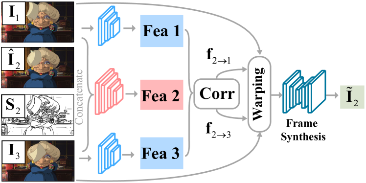
Fig. 4: Framework of the proposed SktFI network.

SktFI aims to refine the initial interpolated image $\mathbf{\hat{I}}_{2}$ using a user-provided sketch $\mathbf{S}_{2}$ as a reference, as shown in Figure 4. The sketch $\mathbf{S}_{2}$ could be generated from the initial interpolated frame using sketch simplification algorithms [15], then the user refines the error-prone synthesized areas.

We first extract features from input $\mathbf{I}_{1}$ and $\mathbf{I}_{3}$ using feature extractor, denoted by $\{\mathbf{Fea}_{1},\mathbf{Fea}_{3}\}$. We the use another extend extractor to extract feature $\mathbf{Fea}_{2}$ from concatenated frames $\{\mathbf{I}_{1},\mathbf{\hat{I}}_{2},\mathbf{S}_{2},\mathbf{I}_{3}\}$. Then the extracted frames are forward into correlation module from [13] to synthesize bidirectional optical flows, denoted by $\mathbf{f}_{2\rightarrow 1}$ and $\mathbf{f}_{2\rightarrow 3}$. Finally, we backward warping $\{\mathbf{I}_{1},\mathbf{\hat{I}}_{2},\mathbf{S}_{2},\mathbf{I}_{3}\}$ guided by estimated flows $\mathbf{f}_{2\rightarrow 1}$ and $\mathbf{f}_{2\rightarrow 3}$ into the intermediate time index, and the a frame synthesis module takes all the warped frames as input to synthesize the refined image $\mathbf{\tilde{I}}_{2}$. The supplementary material provides network details of feature extractors and the frame synthesis module.

3 Experiments

3.1 Dataset

The training data for AutoFI is generated using an animation film (see Section 2.1), called Spirited Away. We synthesize 40K triples with resolution $512\times 384$. The training data for SktFI requires user-provided sketches as inputs. We use the triplet frames from the training set of ATD-12K [9] and use sketch generation pipeline from [16] to synthesize the middle frame sketch. The test set is sampled from ATD-12K. ATD-12K test set includes several files, and we select the frames that contain Spirited Away as our testing data, which contains 313 triples with resolution $960\times 540$. We use PSNR and SSIM as well as LPIPS [17] for quantitative comparisons.

3.2 Loss Function

We aim to enhance frame interpolation networks DAIN [3] (trained on natural video set Vimeo90K [7]) and ANIN [9] (trained on manually collected animation dataset ATD-12K [9]). As shown in Figure 1(b), we utilize the training set generated based on AutoFI to train DAIN and ANIN using $\mathbf{I}_{1},\mathbf{I}_{3}$ as input. We denote the synthesized frame by $\hat{\mathbf{I}}_{2}$. In the AutoFI pipeline, we use pixel reconstruction loss $\mathcal{L}_{C}$ from [3] to train frame interpolation networks. Except for $\mathcal{L}_{C}$, we also adopt perceptual loss $\mathcal{L}_{F}$ from [2] to retain more details in complex cases. For example, the model that we fine-tune ANIN [9] using AutoFI with $\mathcal{L}_{F}$ is denoted by AutoFI -anin -$\mathcal{L}_{F}$. Notice that AutoFI -anin denotes the model using $\mathcal{L}_{C}$, unless otherwise specified. In the SktFI pipeline, we use pixel reconstruction loss $\mathcal{L}_{C}$ to train the refinement network. When training the SktFI module, we fix the weights of the pre-stage frame interpolation module.

-$\mathcal{L}_{C}$
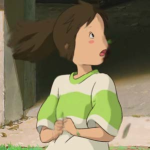
-$\mathcal{L}_{F}$

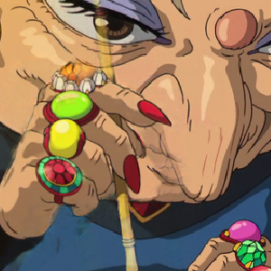
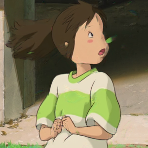
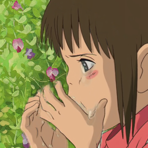
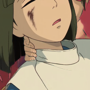
Fig. 5: Analysis of loss functions on AutoFI -anin.

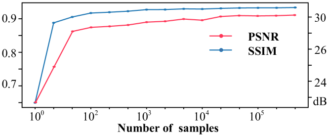
Fig. 6: Performance versus training samples of AutoFI dataset (left, SSIM; right, PSNR).

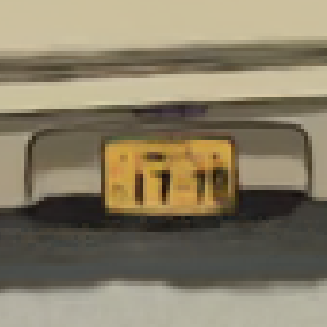
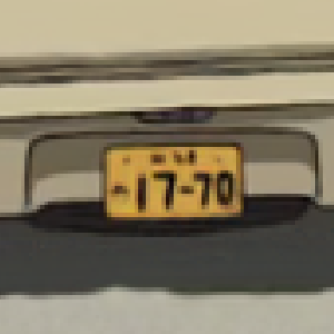
Inputs	GT	BMBC [18]	AdaCoF [19]	DAIN [3]	AutoFI -dain	ANIN [9]	AutoFI -anin

Fig. 7: Visual comparisons of AutoFI. The AutoFI synthesizes sharper and higher-quality interpolated frames.

Table 1: Quantitative comparisons.

Method	PSNR $\uparrow$	SSIM $\uparrow$	LPIPS $\downarrow$
BMBC [18]	27.77	0.9146	0.1025
SepConv [20]	26.87	0.9044	0.1263
AdaCoF [19]	28.29	0.9118	0.1036
DAIN [3]	29.56	0.9272	0.0655
ANIN [9]	29.28	0.9275	0.1036
AutoFI -anin -$\mathcal{L}_{C}$ -w/o b	29.92	0.9314	0.0651
AutoFI -dain -$\mathcal{L}_{C}$	29.61	0.9278	0.0613
AutoFI -anin -$\mathcal{L}_{F}$	29.65	0.9272	0.0611
AutoFI -anin -$\mathcal{L}_{C}$	30.10	0.9334	0.0646
SktFI -none	31.64	0.9421	0.0584
SktFI -dain	31.90	0.9470	0.0506
SktFI -anin	32.22	0.9502	0.0486

3.3 Ablation Experiments

We conduct ablation experiments to evaluate the effectiveness of the proposed method.

Number of Training Steps.

As shown in Figure 6, running more iterations to train AutoFI -anin, such as $10^{4}$, results in moderate gains. When iterations come to $10^{5}$, the model is almost converged.

Loss Function.

The model with perceptual loss (AutoFI -anin -$\mathcal{L}_{F}$) achieve lower PSNR (0.45dB), but better LPIPS index than the model without using $\mathcal{L}_{F}$ (AutoFI -anin -$\mathcal{L}_{C}$), as shown in Table 1. The visual results in Figure 5 show that the perceptual loss can help the model retain more details in difficult areas, resulting in sharper and higher quality frames.

Gaussian Blur on AutoFI.

As shown in Table 1, Gaussian blur on AutoFI brings about $0.18$dB PSNR gain (AutoFI -anin -$\mathcal{L}_{C}$ versus AutoFI -anin -$\mathcal{L}_{C}$ -w/o b ).

Initial Frame on SktFI.

We compare the SktFI module without using initial interpolated frame (denoted by SktFI -none), using initial interpolated frame from AutoFI -dain (denoted by SktFI -dain) and using interpolated frame from AutoFI -anin (denoted by SktFI -anin). As shown in Table 1, SktFI -anin performs favorably against other methods, which means a better initial interpolated frame improve subsequent refinement performance.

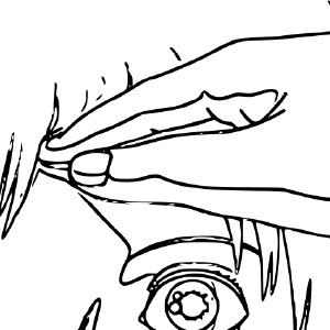
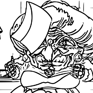
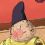
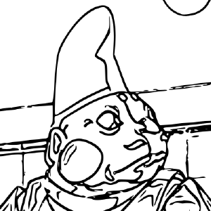
Inputs	GT	AutoFI -anin	SktFI -anin	Sketch

Fig. 8: Visual comparisons of SktFI. SktFI uses the sketch to refine the shape of the intermediate interpolated frame and restore more details.

3.4 Comparisons with State-of-the-arts

We compare the performance of AutoFI and SktFI with state-of-the-art frame interpolation baselines, including BMBC [18], SepConv [20], AdaCoF [19], DAIN [3], ANIN [9].

Numerical Comparisons.

As shown in Table 1, the AutoFI -anin -$\mathcal{L}_{C}$ outperforms all compared baselines, which obtains 0.82dB PSNR against ANIN [9]. Besides, the AutoFI -anin -$\mathcal{L}_{C}$ achieves 0.49dB PSNR gain against AutoFI -dain -$\mathcal{L}_{C}$. The numerical results demonstrate the effectiveness of AutoFI. For the aspect of SktFI, as shown in Table 1, the Skt -anin has best interpolation performance, which obtains about 2dB PSNR gain against AutoFI -anin -$\mathcal{L}_{C}$. The main reason for the high performance of SktFI is that the sketch is drawn from the ground-truth intermediate frame of the test set with nonlinear motion. In contrast, frame interpolation algorithms are under the linear motion assumption. Thus the sketch rectifies the linear interpolated frame to a nonlinear version, which fits the non-linearity of the test set.

Visual Comparisons.

We show visual comparisons of AutoFI in Figure 7. The AutoFI synthesizes sharper and higher-quality interpolated frames. AutoFI ensures the basic assumption of linear motion of frame interpolation algorithms. While the non-linearity of the traditional training set, such as ATD-12K [9] misleads the frame interpolation network, resulting in blurry results. We show visual comparisons of SktFI in Figure 8. The user-provided sketch in SktFI provides the cues of intermediate contours, helping to refine the shape of the intermediate interpolated frame and restore more details.

4 Conclusion

This paper presents AutoFI, an effective method to render training data for deep animation video interpolation. AutoFI takes a layered architecture to render synthetic data, which ensures the assumption of linear motion. Besides AutoFI, we also propose a plug-and-play sketch-based post-processing module, named SktFI, to refine the final results using user-provided sketches manually. AutoFI and SktFI help to improve the animation production pipeline. Numerical and visual results demonstrate that the interpolated animation frames show high-performance and high-perceptual-quality.

References

- [1] Huaizu Jiang, Deqing Sun, Varun Jampani, Ming-Hsuan Yang, Erik Learned-Miller, and Jan Kautz, “Super slomo: High quality estimation of multiple intermediate frames for video interpolation,” in Proceedings of the IEEE Conference on Computer Vision and Pattern Recognition, 2018, pp. 9000–9008.
- [2] Simon Niklaus and Feng Liu, “Softmax splatting for video frame interpolation,” in Proceedings of the IEEE/CVF Conference on Computer Vision and Pattern Recognition, 2020, pp. 5437–5446.
- [3] Wenbo Bao, Wei-Sheng Lai, Chao Ma, Xiaoyun Zhang, Zhiyong Gao, and Ming-Hsuan Yang, “Depth-aware video frame interpolation,” in Proceedings of the IEEE/CVF Conference on Computer Vision and Pattern Recognition, 2019, pp. 3703–3712.
- [4] Wang Shen, Wenbo Bao, Guangtao Zhai, Li Chen, Xiongkuo Min, and Zhiyong Gao, “Blurry video frame interpolation,” in Proceedings of the IEEE/CVF Conference on Computer Vision and Pattern Recognition, 2020, pp. 5114–5123.
- [5] Wang Shen, Wenbo Bao, Guangtao Zhai, Li Chen, Xiongkuo Min, and Zhiyong Gao, “Video frame interpolation and enhancement via pyramid recurrent framework,” IEEE Transactions on Image Processing, vol. 30, pp. 277–292, 2020.
- [6] Wang Shen, Ming Cheng, Guo Lu, Guangtao Zhai, Li Chen, M Salman Asif, and Zhiyong Gao, “Spatial temporal video enhancement using alternating exposures,” IEEE Transactions on Circuits and Systems for Video Technology, 2021.
- [7] Tianfan Xue, Baian Chen, Jiajun Wu, Donglai Wei, and William T Freeman, “Video enhancement with task-oriented flow,” International Journal of Computer Vision, vol. 127, no. 8, pp. 1106–1125, 2019.
- [8] Shuochen Su, Mauricio Delbracio, Jue Wang, Guillermo Sapiro, Wolfgang Heidrich, and Oliver Wang, “Deep video deblurring for hand-held cameras,” in Proceedings of the IEEE Conference on Computer Vision and Pattern Recognition, 2017, pp. 1279–1288.
- [9] Li Siyao, Shiyu Zhao, Weijiang Yu, Wenxiu Sun, Dimitris Metaxas, Chen Change Loy, and Ziwei Liu, “Deep animation video interpolation in the wild,” in Proceedings of the IEEE/CVF Conference on Computer Vision and Pattern Recognition, 2021, pp. 6587–6595.
- [10] John YA Wang and Edward H Adelson, “Representing moving images with layers,” IEEE transactions on image processing, vol. 3, no. 5, pp. 625–638, 1994.
- [11] Deqing Sun, Erik Sudderth, and Michael Black, “Layered image motion with explicit occlusions, temporal consistency, and depth ordering,” Advances in Neural Information Processing Systems, vol. 23, pp. 2226–2234, 2010.
- [12] Deqing Sun, Daniel Vlasic, Charles Herrmann, Varun Jampani, Michael Krainin, Huiwen Chang, Ramin Zabih, William T Freeman, and Ce Liu, “Autoflow: Learning a better training set for optical flow,” in Proceedings of the IEEE/CVF Conference on Computer Vision and Pattern Recognition, 2021, pp. 10093–10102.
- [13] Deqing Sun, Xiaodong Yang, Ming-Yu Liu, and Jan Kautz, “Pwc-net: Cnns for optical flow using pyramid, warping, and cost volume,” in Proceedings of the IEEE conference on computer vision and pattern recognition, 2018, pp. 8934–8943.
- [14] Zachary Teed and Jia Deng, “Raft: Recurrent all-pairs field transforms for optical flow,” in European conference on computer vision. Springer, 2020, pp. 402–419.
- [15] Edgar Simo-Serra, Satoshi Iizuka, and Hiroshi Ishikawa, “Mastering sketching: Adversarial augmentation for structured prediction,” ACM TOG, vol. 37, no. 1, pp. 1–13, 2018.
- [16] Tiziano Portenier, Qiyang Hu, Attila Szabo, Siavash Arjomand Bigdeli, Paolo Favaro, and Matthias Zwicker, “Faceshop: Deep sketch-based face image editing,” ACM Transactions on Graphics, vol. 37, pp. 99, 2018.
- [17] Richard Zhang, Phillip Isola, Alexei A Efros, Eli Shechtman, and Oliver Wang, “The unreasonable effectiveness of deep features as a perceptual metric,” in Proceedings of the IEEE conference on computer vision and pattern recognition, 2018, pp. 586–595.
- [18] Junheum Park, Keunsoo Ko, Chul Lee, and Chang-Su Kim, “Bmbc: Bilateral motion estimation with bilateral cost volume for video interpolation,” in Computer Vision–ECCV 2020: 16th European Conference, Glasgow, UK, August 23–28, 2020, Proceedings, Part XIV 16. Springer, 2020, pp. 109–125.
- [19] Hyeongmin Lee, Taeoh Kim, Tae-young Chung, Daehyun Pak, Yuseok Ban, and Sangyoun Lee, “Adacof: Adaptive collaboration of flows for video frame interpolation,” in Proceedings of the IEEE/CVF Conference on Computer Vision and Pattern Recognition, 2020, pp. 5316–5325.
- [20] Simon Niklaus, Long Mai, and Oliver Wang, “Revisiting adaptive convolutions for video frame interpolation,” in Proceedings of the IEEE/CVF Winter Conference on Applications of Computer Vision, 2021, pp. 1099–1109.