Modeling Continuous Time Sequences with Intermittent Observations using Marked Temporal Point Processes

Abstract.

A large fraction of data generated via human activities such as online purchases, health records, spatial mobility etc. can be represented as a sequence of events over a continuous-time. Learning deep learning models over these continuous-time event sequences is a non-trivial task as it involves modeling the ever-increasing event timestamps, inter-event time gaps, event types, and the influences between different events within and across different sequences. In recent years neural enhancements to marked temporal point processes (MTPP) have emerged as a powerful framework to model the underlying generative mechanism of asynchronous events localized in continuous time. However, most existing models and inference methods in the MTPP framework consider only the complete observation scenario i.e. the event sequence being modeled is completely observed with no missing events – an ideal setting that is rarely applicable in real-world applications. A recent line of work which considers missing events while training MTPP utilizes supervised learning techniques that require additional knowledge of missing or observed label for each event in a sequence, which further restricts its practicability as in several scenarios the details of missing events is not known apriori. In this work, we provide a novel unsupervised model and inference method for learning MTPP in presence of event sequences with missing events. Specifically, we first model the generative processes of observed events and missing events using two MTPP, where the missing events are represented as latent random variables. Then, we devise an unsupervised training method that jointly learns both the MTPP by means of variational inference. Such a formulation can effectively impute the missing data among the observed events, which in turn enhances its predictive prowess, and can identify the optimal position of missing events in a sequence. Experiments with eight real-world datasets show that IMTPP outperforms the state-of-the-art MTPP frameworks for event prediction, missing data imputation, and provides stable optimization.

1. Introduction

The amount of data constantly generated via several human activities has grown exponentially with time-series becoming pervasive across all such activities ranging from finance, social, online purchases, and many more (Shieh and Keogh, 2008; Rakthanmanon et al., 2012; Mueen and Keogh, 2016). Learning the dynamics of these sequences is a non-trivial task with the current neural models as it requires perpetual modeling of continuous-time and inter-event relationships (Du et al., 2016; Zhang et al., 2020; Kumar et al., 2019). In the recent years, marked temporal point processes (MTPP) (Valera et al., 2014; Rizoiu et al., 2017; Wang et al., 2017; Daley and Vere-Jones, 2007) have shown an outstanding potential to characterize asynchronous events localized in continuous time that appear in a wide range of applications in healthcare (Lorch et al., 2018; Rizoiu et al., 2018; Gupta et al., 2022), traffic (Du et al., 2016; Guo et al., 2018), web and social networks (Valera et al., 2014; Du et al., 2015; Tabibian et al., 2019; Kumar et al., 2019; De et al., 2016; Du et al., 2016; Farajtabar et al., 2017; Jing and Smola, 2017; Likhyani et al., 2020), finance (Bacry et al., 2015), activity sequences (Gupta and Bedathur, 2022b; Mehrasa et al., 2019) and many more.

A temporal point process represents an event using two quantities: (i) the time of its occurrence and (ii) the associated mark, where the latter indicates the category of the event and therefore bears different meanings for different applications. For example, in a social network setting, the marks may indicate users’ likes, topics, and opinions of the posts; in finance, they may correspond to the stock prices and the number of sales; in healthcare, they may indicate the state of the disease of an individual. In this context, most of the MTPP models (Valera et al., 2014; Wang et al., 2017; Huang et al., 2019; Du et al., 2016; Zuo et al., 2020; Zhang et al., 2020)— with a few recent exceptions (Shelton et al., 2018; Mei et al., 2019)— have considered only the settings where the training data is completely observed or, in other words, there is no missing observation at all. While working with fully observed data is ideal for understanding any dynamical system, this is not possible in many practical scenarios. We may miss observing events due to constraints such as crawling restrictions by social media platforms, privacy restrictions (certain users may disallow collection of certain types of data), budgetary factors such as data collection for exit polls, or other practical factors e.g. a patient may not be available at a certain time. This results in the poor predictive performance of MTPP models (Du et al., 2016; Zuo et al., 2020; Zhang et al., 2020) that skirt this issue.

Statistical analysis in presence of missing data has been widely researched in literature in various contexts  (Che et al., 2016; Yoon et al., 2018; Tian et al., 2018; Smieja et al., 2018). Little and Rubin (2019) offer a comprehensive survey. It provides three models that capture data missing mechanisms in the increasing order of complexity, viz., MCAR (missing completely at random), MAR (missing at random), and MNAR (missing not at random). Recently,  Shelton et al. (2018) and Mei et al. (2019) proposed novel methods to impute missing events in continuous-time sequences via MTPP from the viewpoint of the MNAR mechanism. However, they focus on imputing missing data in between a-priori available observed events, rather than predicting observed events in the face of missing events. Moreover, they deploy expensive learning and sampling mechanisms, which make them often intractable in practice, especially in the case of learning from a sequence of streaming events. For example, Shelton et al. (2018) apply an expensive MCMC sampling procedure to draw missing events between the observation pairs, which requires several simulations of the sampling procedure upon arrival of a new sample. On the other hand, Mei et al. (2019) uses bi-directional RNN which re-generates all missing events by making a completely new pass over the backward RNN, whenever one new observation arrives. As a consequence, it suffers from quadratic complexity with respect to the number of observed events. On the other hand, the proposal of Shelton et al. (2018) depends on a pre-defined influence structure among the underlying events, which is available in linear multivariate parameterized point processes. In more complex point processes with neural architectures, such a structure is not explicitly defined, which further limits their applicability in real-world settings.

1.1. Present Work

In this work, we overcome the above limitations by devising a novel modeling framework for point processes called IMTPP (Intermittently-observed Marked Temporal Point Processes) , which characterizes the dynamics of both observed and missing events as two coupled MTPP, conditioned on the history of previous events. In our setup, the generation of missing events depends both on the previously occurred missing events as well as the previously occurred observed events. Therefore, they are MNAR (missing not at random), in the context of the literature of missing data (Little and Rubin, 2019). In contrast to the prior models (Mei et al., 2019; Shelton et al., 2018), IMTPP aims to learn the dynamics of both observed and missing events, rather than simply imputing missing events in between the known observed events, which is reflected in its superior predictive power over those existing models.

Precisely, IMTPP represents the missing events as latent random variables, which together with the previously observed events, seed the generative processes of the subsequent observed and missing events. Then it deploys three generative models— MTPP for observed events, prior MTPP for missing events, and posterior MTPP for missing events, using recurrent neural networks (RNN) that capture the nonlinear influence of the past events. We also show that such a formulation can be easily extended to imputation tasks and still achieve significant performance gains over other models. IMTPP includes several technical innovations over other models, that significantly boost its training efficiency as well as its event prediction accuracy. We list them here:

1. In a notable departure from almost all existing MTPP models (Du et al., 2016; Tabibian et al., 2019; Mei et al., 2019; De et al., 2016) which rely strongly on conditional intensity functions, we use a log-normal distribution to sample arrival times of the events. As suggested by Shchur et al. (2020), such distribution allows efficient sampling as well as a more accurate prediction than the standard intensity function-based models.

2. The built-in RNNs in our model are designed to make forward computations. Therefore, they incrementally update the dynamics upon the arrival of a new observation. Consequently, unlike the prior models, it does not require to re-generate all the missing events responding to the arrival of an observation, which significantly boosts the efficiency of both learning and prediction as compared to both the previous approaches (Mei et al., 2019; Shelton et al., 2018).

Our modeling framework allows us to train IMTPP using an efficient variational inference method, that maximizes the evidence lower bound (ELBO) of the likelihood of the observed events. Such a formulation highlights the connection of our model with the variational autoencoders (VAEs) (Chung et al., 2015; Bowman et al., 2015). However, in sharp contrast to traditional VAEs, where the random noises or seeds often do not have immediate interpretations, our random variables bear concrete physical explanations i.e. they are missing events, which renders our model more explainable than an off-the-shelf VAE. In addition, to further elucidate the predictive prowess of IMTPP, we constrain its optimization procedure to identify the optimal positions of missing events in a sequence.

Finally, we perform exhaustive experiments with six diverse real-world datasets across different domains to show that IMTPP can model missing observations within a stream of observed events and enhance the predictive power of the original generative process for a full observation scenario.

1.2. Organization

The rest of this paper is organized as follows. We review the relevant related work in Section 2 and present a formal problem formulation in Section 3, followed by an overview of IMTPP— including the description of coupled MTPP based model — in Section 4. Section 5 gives a detailed development of all components in IMTPP and Section 6 contains in-depth experimental analysis, qualitative, and imputation studies over all datasets before concluding in Section 7.

2. Related Work

Our work is broadly related to the literature of (i) temporal point process, (ii) missing data models for discrete-time series, and (iii) missing data models for temporal point process.

2.1. Marked Temporal Point Process

Marked Temporal point processes are central to our work. In recent years, they emerged as a powerful tool to model asynchronous events localized in continuous time (Daley and Vere-Jones, 2007; Hawkes, 1971), which have a wide variety of applications e.g., information diffusion, disease modeling, finance, etc. Driven by these motivations, in recent years, there has been a surge of works on MTPP (Rizoiu et al., 2017; Rizoiu et al., 2018; Du et al., 2015; Farajtabar et al., 2017). They predominantly follow two approaches. The first approach which includes the Hawkes process, self-correcting process, etc. considers fixed parameterization of the temporal point process. Here, different parameterizations characterize the phenomena of interest. In particular, Hawkes process models the self-exciting event arrival process, which is often exhibited by online social networks. However, the fixed parameterization approach often constrains the expressive power of the underlying model, which is often reflected in the sub-optimal predictive performance. The second approach aims to overcome these challenges by modeling MTPP with a deep neural network (Du et al., 2016; Mei and Eisner, 2017; Xiao et al., 2017b; Huang et al., 2019). For example, Du et al. (2016) proposed recurrent marked temporal point process (RMTPP)— an RNN driven model— to encapsulate the sequence dynamics and obtain a low dimensional embedding of the event history. This led to further developments which include the Neural Hawkes process that formulates the point process with a continuous-time LSTM (Mei and Eisner, 2017) and several other neural models of MTPP e.g., (Xiao et al., 2017b; Huang et al., 2019; Omi et al., 2019). However, these approaches assume that the underlying data fed into the model is complete, i.e., with no missing entries. This assumption of an ideal setting leads to conjectured predictions if implemented in presence of missing data.

2.2. Missing Data Models for Discrete-Time Series

Our current work is also related to existing missing data models for discrete time-series, which do not necessarily consider MTPP. In principle, training sequential models in presence of missing data is essential for robust predictions across a wide range of applications e.g., traffic networks (Tian et al., 2018), modeling disease propagation (Bai et al., 2018; Ghazi et al., 2019) and wearable sensor data (Wu et al., 2018; Wu et al., 2020). Motivated by these applications, in recent years, there has been a considerable effort in designing learning tools for sequence models with missing data (Che et al., 2016; Yoon et al., 2018; Luo et al., 2018). In particular, the proposal by Che et al. (2016) compensate for a missing event by applying a time decay factor to the previous hidden state in a GRU before calculating the new hidden state. Yoon et al. (2018) capture the effect of missing data by incorporating future information using bidirectional-RNNs. While these approaches do not provide explicit generative models of missing events, few other models generate them by imputing them in between available observations. For example, Cao et al. (2018) proposed a method of imputing missing events using a bi-directional RNN (Cao et al., 2018); Luo et al. (2018) employs a generative adversarial approach for generating missing events conditioned on the observed events. Luo et al. (2019) and Li et al. (2018b) are used for imputing in time-series, however, cannot be used to sample marks of missing events and thus, cannot be extended to imputation in continuous-time event sequences. Thus, these models are complementary to our proposal as they do not work with temporal point processes.

2.3. Missing Data Models for Temporal Point Process

Very recently, there has been a growing interest in modeling MTPP in presence of missing observations. However, the design of their learning paradigms is tailored too much to operate in an offline setting. They deploy expensive learning and sampling mechanisms on an apriori-known complete sequence of observations. More specifically, Shelton et al. (2018) proposed a way of incorporating missing data by generating children events for the observed events. They rely strongly on an expensive MCMC sampling procedure to draw missing events between the observation pairs. In order to adapt such a protocol, we need to run the entire sampling routine several times whenever a new observation arrives. Such a method is extremely time-consuming and often intractable in practice. Moreover, they require an underlying multi-variate parenthood structure which is not available in a complicated neural setting. Our work is closely related to the proposal by Mei et. al. (Mei et al., 2019). It employs two RNNs, in which, the forward RNN— initialized on $t=0$—models the observation sequence and the backward RNN— initialized on $t=T$— models the missing observations. To operate a backward RNN in an online setting, we need to pass the entire sequence of observations into it, whenever a new sample arrives, which in turn makes it super expensive in practice. While re-running these methods after batch arrivals— instead of re-running after every single arrival— may appear as a compromised solution, however, that is ineffective in practice. Other approaches include the proposal by Xu et al. (2017), which proposes a training method for MTPP when the future and past events of a sequence window are censored; the work by  Rasmussen (2013), which assumes certain characteristics of missing data, and Zhuang et al. (2020) is limited to spatial modeling.

3. Problem setup

In this section, we first introduce the notations and then the setup of our problem of learning marked temporal point processes with observed and missing events over continuous time.

3.1. Preliminaries and Notations

A marked temporal point process (MTPP) is a stochastic process whose realization consists of a sequence of discrete localized in time. Formally, we characterize an MTPP using the sequence of observed events $\mathcal{S}_{k}=\{e_{i}=(x_{i},t_{i})|i\in[k],t_{i}<t_{i+1}\}$, where $t_{i}\in\mathbb{R}^{+}$ is the time of occurrence and $x_{i}\in\mathcal{C}$ is a discrete mark of the $i$-th observed event that occurred at time $t_{i}$, with $\mathcal{C}$ to be the set of discrete marks. Here, $\mathcal{S}_{k}$ denotes the sequence with first $k$ observed events. We denote the inter-arrival times of the observed events as, $\Delta_{t,k}=t_{k}-t_{k-1}$.

However as highlighted in Section 1, there may be instances where an event has actually taken place, but not recorded with the observed event sequence $\mathcal{S}$. To this end, we introduce the MTPP for missing events— a latent MTPP— which is characterized by a sequence of hidden events $\mathcal{M}_{r}=\{\epsilon_{j}=(y_{j},\tau_{j})|j\in[r],\tau_{j}<\tau_{j+1}\}$ where $\tau_{j}\in\mathbb{R}^{+}$ and $y_{j}\in\mathcal{C}$ are the times and the marks of the $j$-th missing events. Therefore, $\mathcal{M}_{r}$ defines the set of first $r$ missing events. Moreover, we denote the inter-arrival times of the missing events as, $\Delta_{\tau,r}=\tau_{r}-\tau_{r-1}$.

Note that $\tau_{\bullet}$, $y_{\bullet}$, $\mathcal{M}_{\bullet}$ and $\Delta_{\tau,\bullet}$ for the MTPP of missing events share similar meanings with $t_{\bullet}$, $x_{\bullet}$, $\mathcal{S}_{\bullet}$ and $\Delta_{t,\bullet}$ respectively for the MTPP of observed events. For an intelligible description of our model, we further define two critical notations $\underline{k}$ and $\overline{k}$ as follows:

(1) $$\underline{k} =\mathop{\mathrm{argmin}}_{r}\{\tau_{r}\,|\,t_{k}<\tau_{r}<t_{k+1}\}$$

(2) $$\ \overline{k} =\mathop{\mathrm{argmax}}_{r}\{\tau_{r}\,|\,t_{k}<\tau_{r}<t_{k+1}\}$$

Here, $\underline{k}$ and $\overline{k}$ are the indices of the first and the last missing events respectively, among those which have arrived between $k$-th and $k+1$-th observed events. Figure 2 (a) illustrates our setup.

In practice, the arrival times ($t$ and $\tau$) of both observed and missing events are continuous random variables, whereas the marks ($x$ and $y$) are discrete random variables. Therefore, following the state-of-the-art MTPP models (Du et al., 2016; Mei and Eisner, 2017), we model a density function to draw the event timings and a probability mass function to draw marks, which in turn induce a net density function characterizing the generative process.

3.2. Our Distinctive Goal

Our goal in this paper is to design an MTPP model which can generate the subsequent observed ($e_{k+1}$) and missing events ($\epsilon_{r+1}$) in a recursive manner, conditioned on the history of all events $\mathcal{S}_{k}\cup\mathcal{M}_{r}$ that have occurred thus far.

Given the input sequence of observations $\mathcal{S}_{K}$ consisting of first $K$ observed events $\{e_{1},e_{2},...,e_{K}\}$, we first train our generative model and then recursively predict the next observed event $e_{K+1}$. Though IMTPP can also predict the missing events but we evaluate the predictive performance only on observed events since the missing events are not available in practice. We also evaluate the imputation performance of our model by predicting synthetically deleted events.

Note that, this setting is in contrast to the proposal of (Mei et al., 2019) that aims to impute the missing events based on the entire observation sequence $\mathcal{S}_{K}$ using a bi-directional RNN. Specifically, whenever one new observation arrives, it re-generates all missing events by making a completely new pass over the backward RNN. As a consequence, such an imputation method not only suffers from the quadratic complexity with respect to the number of observed events it also has limited practicability as in a streaming or an online setting the future events are also not available beyond the current timestamp. Furthermore, their approach is tailored towards imputing missing events based on the complete observations and not well suited to predict observed events in the face of missing observations. In contrast, our proposal is designed to generate subsequent observed and missing events in between previously observed events. Therefore, it does not require to re-generate all missing events whenever a new observation arrives, which allows it to enjoy a linear complexity with respect to the number of observed events and can be easily extended to online settings.

4. Components of IMTPP

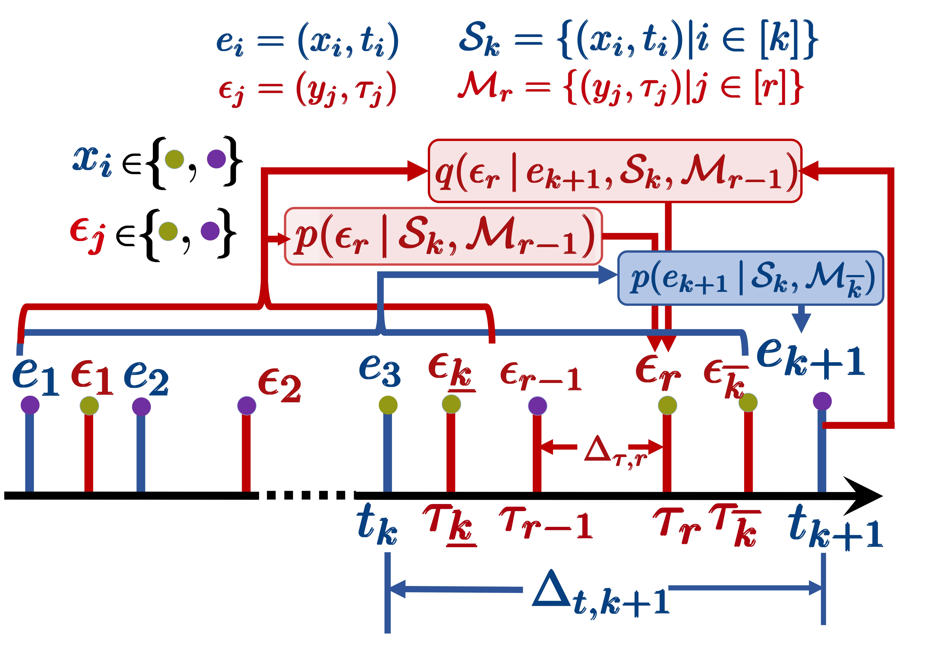
Figure 1. Overall neural architecture of IMTPP. The figure illustrates the notations, the observed, and missing point processes in IMTPP. The components concerning observed events and missing events are marked with blue and red respectively. The figure also illustrates the generation process for events $e_{k+1}$ and $\epsilon_{r}$.

At the very outset, IMTPP, our proposed generative model, connects two stochastic processes— one for the observed events, which samples the observed and the other for the missing events— based on the history of previously generated missing and observed events. Note, that the sequence of training events that are given as input to IMTPP consists of only the observed events. We model the missing event sequence through latent random variables, which, along with the previously observed events, drive a unified generative model for the complete (observed and missing) event sequence. The overall neural architecture of IMTPP, including the different processes for observed and missing events is given in Figure 1.

More specifically, given a stream of observed events $\mathcal{S}_{K}=\{e_{1}=(x_{1},t_{1}),e_{2}=(x_{2},t_{2}),\ldots,e_{K}=(x_{K},t_{K})\}$, if we use the maximum likelihood principle to train IMTPP, then we should maximize the marginal log-likelihood of the observed stream of events, i.e., $\log p(\mathcal{S}_{K})$. However, computation of $\log p(\mathcal{S}_{K})$ demands marginalization with respect to the set of latent missing events $\mathcal{M}_{\overline{K-1}}$, which is typically intractable. Therefore, we resort to maximizing a variational lower bound or evidence lower bound (ELBO) of the log-likelihood of the observed stream of events $\mathcal{S}_{K}$. Mathematically, we note that:

$$p(\mathcal{S}_{K})=\prod_{k=0}^{K-1}\int_{\mathcal{M}_{\overline{k}}}p(e_{k+1}\,|\,\mathcal{S}_{k},\mathcal{M}_{\overline{k}})\,p(\mathcal{M}_{\overline{k}})\,d\omega(\mathcal{M}_{\overline{k}})$$

(3) $$=\mathbb{E}_{q(\mathcal{M}_{\overline{K-1}}\,|\,\mathcal{S}_{K})}\prod_{k=0}^{K-1}\frac{p(e_{k+1}\,|\,\mathcal{S}_{k},\mathcal{M}_{\overline{k}})\displaystyle\prod_{r=\underline{k}}^{\overline{k}}p(\epsilon_{r}\,|\,\mathcal{S}_{k},\mathcal{M}_{r-1})}{\displaystyle\prod_{r=\underline{k}}^{\overline{k}}q(\epsilon_{r}\,|\,e_{k+1},\mathcal{S}_{k},\mathcal{M}_{r-1})}$$

where, $\omega(\mathcal{M})$ is the measure of the set $\mathcal{M}$, $q$ is an approximate posterior distribution which aims to interpolate missing events $\epsilon_{r}$ within the interval $(t_{k},t_{k+1})$, based on the knowledge of the next observed event $e_{k}$, along with all previous events $\mathcal{S}_{k}\cup\mathcal{M}_{r-1}$, and $\underline{k}$, $\overline{k}$. Recall that $\underline{k}$ $(\overline{k})$ is the index $r$ of the first (last) missing event $\epsilon_{r}$ among those which have arrived between $k$-th and $k+1$-th observed events, i.e., $\underline{k}=\mathop{\mathrm{argmin}}_{r}\{\tau_{r}\,|\,t_{k}<\tau_{r}<t_{k+1}\}$ and $\overline{k}=\mathop{\mathrm{argmax}}_{r}\{\tau_{r}\,|\,t_{k}<\tau_{r}<t_{k+1}\}$. Next, by applying Jensen inequality over the likelihood function, $\log p(\mathcal{S}_{K})$ is at-least:

(4) $$\mathbb{E}_{q(\mathcal{M}_{\overline{K-1}\,|\,\mathcal{S}_{K}})}\sum_{k=0}^{K-1}\log p(e_{k+1}\,|\,\mathcal{S}_{k},\mathcal{M}_{\overline{k}})-\sum_{k=0}^{K-1}\sum_{r=\underline{k}}^{\overline{k}}\text{KL}\bigg{[}q(\epsilon_{r}\,|\,e_{k+1},\mathcal{S}_{k},\mathcal{M}_{r-1})||p(\epsilon_{r}\,|\,\mathcal{S}_{k},\mathcal{M}_{r-1})\bigg{]},$$

While the above inequality holds for any distribution $q$, the quality of this lower bound depends on the expressivity of $q$, which we would model using a deep recurrent neural network. Moreover, the above lower bound suggests that our model consists of the following components.

1. MTPP for observed events. The distribution $p(e_{k+1}\,|\,\mathcal{S}_{k},\mathcal{M}_{\overline{k}})$ models the MTPP for observed events, which generates the $(k+1)$-th event, $e_{k+1}$, based on the history of all $k$ observed events $\mathcal{S}_{k}$ and all missing events $\mathcal{M}_{\overline{k}}$ generated so far.

2. Prior MTPP for missing events. The distribution $p(\epsilon_{r}\,|\,\mathcal{S}_{k},\mathcal{M}_{{r-1}})$ is the prior model of the MTPP for missing events. It generates the $r$-th missing event $\epsilon_{r}$ after the observed event $e_{k}$, based on the prior information— the history with all $k$ observed events $\mathcal{S}_{k}$ and all missing events $\mathcal{M}_{{r-1}}$ generated so far.

3. Posterior MTPP for missing events. Given the set of observed events $\mathcal{S}_{k+1}=\{e_{1},e_{2},\ldots,e_{k+1}\}$, the distribution $q(\epsilon_{r}\,|\,e_{k+1},\mathcal{S}_{k},\mathcal{M}_{{r-1}})$ generates the $r$-th missing event $\epsilon_{r}$, after the knowledge of the subsequent observed event $e_{k+1}$ is taken into account, along with information about all previously observed events $\mathcal{S}_{k}$ and all missing events $\mathcal{M}_{{r-1}}$ generated so far.

5. Architecture of IMTPP

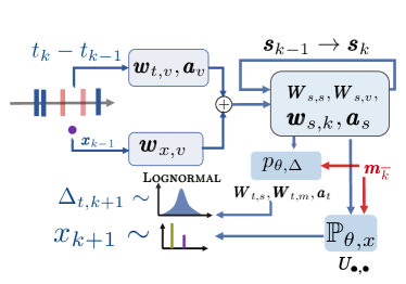
(a) MTPP for observations $p_{\theta}$

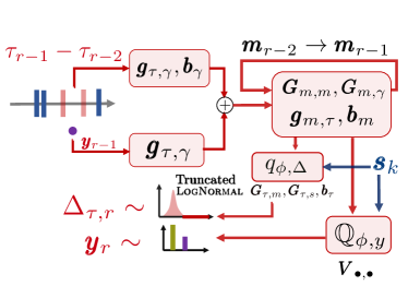
(b) Posterior MTPP for missing events $q_{\phi}$

Figure 2. Architecture of different processes in IMTPP. Panel (a) shows the neural architecture of the MTPP of observations $p_{\theta}$. Panel (b) shows the neural architecture of the posterior MTPP of missing events $q_{\phi}$. Note that, the information of $e_{k+1}$ here is used to truncate the log-normal distribution for missing data generation, whereas the log-normal distribution for observed is non-truncated.

We first present a high-level overview of deep neural network parameterization of different components of IMTPP model and then describe component-wise architecture in detail. Finally, we briefly present the salient features of our proposal.

5.1. High-level Overview

We parameterize different components of IMTPP, introduced in the previous section using deep neural networks. More specifically, we approximate the MTPP for observed events, $p(e_{k+1}\,|\,\mathcal{S}_{k},\mathcal{M}_{\overline{k}})$ using $p_{\theta}$ and the posterior MTPP for missing events $q(\epsilon_{r}\,|\,e_{k+1},\mathcal{S}_{k},\mathcal{M}_{{r-1}})$ using $q_{\phi}$, both implemented as neural networks with parameters $\theta$ and $\phi$ respectively. We set the prior MTPP for missing events $p(\epsilon_{r}\,|\,\mathcal{S}_{k},\mathcal{M}_{{r-1}})$ as a known distribution $p_{{\text{prior}}}$ using the history of all the events it is conditioned on. In this context, we design two recurrent neural networks (RNNs) which embed the history of observed events $\mathcal{S}$ into the hidden vectors $\bm{s}$ and the missing events $\mathcal{M}$ into the hidden vector $\bm{m}$, similar to several state-of-the art MTPP models (Du et al., 2016; Mei and Eisner, 2017; Mei et al., 2019). In particular, the embeddings $\bm{s}_{k}$ and $\bm{m}_{r}$ encode the influence of the arrival time and the mark of the first $k$ observed events from $\mathcal{S}_{k}$ and first $r$ missing events from $\mathcal{M}_{r}$ respectively. Therefore, we can represent the model for predicting the next observed event as:

(5) $$p(e_{k+1}\,|\,\mathcal{S}_{k},\mathcal{M}_{\overline{k}})=p_{\theta}(e_{k+1}\,|\,\bm{s}_{k},\bm{m}_{\overline{k}}).$$

Following the above MTPP model for observed events, both the prior MTPP model and the posterior MTPP model for missing events offer similar conditioning with respect to $\bm{s}_{\bullet}$ and $\bm{m}_{\bullet}$. Similar to other MTPP models (Du et al., 2016; Mei and Eisner, 2017), the RNN for the observed events updates $\bm{s}_{k-1}$ to $\bm{s}_{k}$ by incorporating the effect of $e_{k}$. Similarly, the RNN for the missing events updates $\bm{m}_{r-1}$ to $\bm{m}_{r}$ by taking into account of the event $\epsilon_{r}$.

As mentioned in Section 3, each event has two components, its mark and the arrival-time, which are discrete and continuous random variables respectively. Therefore, we characterize the event distribution as a density function which is the product of the density function ($p_{\theta,\Delta},q_{\phi,\Delta},p_{{\text{prior}},\Delta}$) of the inter-arrival time and the probability distribution ($\mathbb{P}_{\theta,x},\mathbb{Q}_{\phi,y},\mathbb{P}_{{\text{prior}},y}$) of the mark, i.e.,

(6) $$p_{\theta}(e_{k+1}=(x_{k+1},t_{k+1})\,|\,\mathcal{S}_{k},\mathcal{M}_{\overline{k}})=\mathbb{P}_{\theta,x}(x_{k+1}\,|\,\Delta_{t,k+1},\bm{s}_{k},\bm{m}_{\overline{k}})\bm{\cdot}p_{\theta,\Delta}(\Delta_{t,k+1}\,|\,\bm{s}_{k},\bm{m}_{\overline{k}}),$$

(7) $$q_{\phi}(\epsilon_{r}=(y_{r},\tau_{r})\,|\,e_{k+1},\mathcal{S}_{k},\mathcal{M}_{{r-1}})=\mathbb{Q}_{\phi,y}(y_{r}\,|\,\Delta_{\tau,r},e_{k+1},\bm{s}_{k},\bm{m}_{{r-1}})\,\bm{\cdot}q_{\phi,\Delta}(\Delta_{\tau,r}\,|\,e_{k+1},\bm{s}_{k},\bm{m}_{{r-1}}),$$

(8) $$p_{{\text{prior}}}(\epsilon_{r}=(y_{r},\tau_{r})\,|\,\mathcal{S}_{k},\mathcal{M}_{{r-1}})=\mathbb{P}_{{\text{prior}},y}(y_{r}\,|\,\Delta_{\tau,r},\bm{s}_{k},\bm{m}_{{r-1}})\cdot p_{{\text{prior}},\tau}(\Delta_{\tau,r}\,|\,\bm{s}_{k},\bm{m}_{{r-1}}),$$

where, as mentioned, the inter-arrival times $\Delta_{t,k}$ and $\Delta_{\tau,r}$ are given as $\Delta_{t,k}=t_{k}-t_{k-1}$ and $\Delta_{r}=\tau_{r}-\tau_{r-1}$. Moreover, $p_{\theta,\Delta}$, $q_{\phi,\Delta}$ and $p_{{\text{prior}},\Delta}$ denote the density of the inter-arrival times for the observed events, posterior density and the prior density of the inter-arrival times of the missing events; and, $\mathbb{P}_{\theta,x}$, $\mathbb{Q}_{\phi,y}$ and $\mathbb{P}_{{\text{prior}},y}$ denote the corresponding probability mass functions of the mark distributions. Figure 2 denotes the neural architecture of the MTPP for observed events and the posterior MTPP for missing events in IMTPP. For brevity, we omitted the schematic diagram for the prior MTPP for missing events as it had a simpler architecture.

5.2. Parameterization of $p_{\theta}$

Given $k$ observed events and $r=\overline{k}$ missing events, the generative model $p_{\theta}$ samples the next event $e_{k+1}$ based on $\mathcal{S}_{k}$ and $\mathcal{M}_{r}$. To this aim, the underlying neural network takes the embedding vectors $\bm{h}$ and $\bm{s}$ as input and provides the density $p_{\theta,\Delta}$ and $\mathbb{P}_{\theta,x}$ as output, which in turn are used to draw the event $e_{k+1}$. More specifically, we realize $p_{\theta}$ in Eq. 6 using a three layer architecture.

1. Input layer. The first level is the input layer, which takes the last event as input and represents it through a suitable vector. In particular, upon arrival of $e_{k}$, it computes the corresponding vector $\bm{v}_{k}$ as:

   (9) $$\bm{v}_{k}=\bm{w}_{t,v}t_{k}+\bm{w}_{x,v}x_{k}+\bm{w}_{t,\Delta}(t_{k}-t_{k-1})+\bm{a}_{v},$$

   where $\bm{w}_{\bullet,\bullet}$ and $\bm{a}_{v}$ are trainable parameters.

2. Hidden layer The next level is the hidden layer that embeds the sequence of observations into finite dimensional vectors $\bm{s}_{\bullet}$, computed using RNN. Such a layer takes $\bm{v}_{i}$ as input and feed it into an RNN to update its hidden states in the following way.

   (10) $$\bm{s}_{k}=\tanh(\bm{W}_{s,s}\bm{s}_{k-1}+\bm{W}_{s,v}\bm{v}_{k}+(t_{k}-t_{k-1})\bm{w}_{s,k}+\bm{a}_{s}),$$

   where $\bm{W}_{s,\bullet}$ and $\bm{a}_{s}$ are trainable parameters. This hidden state $\bm{s}_{k}$ can also be considered as a sufficient statistic of $\mathcal{S}_{k}$, the sequence of the first $k$ observations.

3. Output layer The next level is the output layer which computes both $p_{\theta,\Delta}(\cdot)$ and $\mathbb{P}_{\theta,x}(\cdot)$ based on $\bm{s}_{k}$ and $\bm{m}_{\overline{k}}$. To this end, we have the density of inter-arrival times as

   (11) $$p_{\theta,\Delta}(\Delta_{t,k+1}\,|\,\bm{s}_{k},\bm{m}_{\overline{k}})=\textsc{Lognormal}\left(\mu_{e}(\bm{s}_{k},\bm{m}_{\overline{k}}),\sigma^{2}_{e}(\bm{s}_{k},\bm{m}_{\overline{k}})\right),$$

   with $[\mu_{e}(\bm{s}_{k},\bm{m}_{\overline{k}}),\sigma_{e}(\bm{s}_{k},\bm{m}_{\overline{k}})]=\bm{W}_{t,s}^{\top}\bm{s}_{k}+\bm{W}_{t,m}^{\top}\bm{m}_{\overline{k}}+\bm{a}_{t}$; and, the mark distribution as,

   (12) $$\mathbb{P}_{\theta,x}(x_{k+1}=x\,|\,\Delta_{t,k+1},\bm{s}_{k},\bm{m}_{\overline{k}})=\frac{\exp(\bm{U}_{x,s}^{\top}\bm{s}_{k}+\bm{U}_{x,m}^{\top}\bm{m}_{\overline{k}})}{\sum_{x^{\prime}\in\mathcal{C}}\exp(\bm{U}_{x^{\prime},s}^{\top}\bm{s}_{k}+\bm{U}_{x^{\prime},m}^{\top}\bm{m}_{\overline{k}})},$$

   The distributions are finally used to draw the inter-arrival time $\Delta_{t,k+1}$ and the mark $x_{k+1}$ for the event $e_{k+1}$. The sampled inter-arrival time $\Delta_{t,k+1}$ gives $t_{k+1}=t_{k}+\Delta_{t,k}$. Here, the mark distribution is independent of $\Delta_{t,k+1}$.

Finally, we note that $\theta=\{\bm{W}_{\bullet,\bullet},\bm{w}_{\bullet,\bullet},\bm{U}_{\bullet,\bullet},\bm{a}_{\bullet}\}$ are trainable parameters.

We would like to highlight that, the proposed lognormal distribution of inter-arrival times $\Delta_{t,k}$ allows an easy re-parameterization trick— $\textsc{Lognormal}(\mu_{e},\sigma_{e})=\exp(\mu_{e}+\sigma_{e}\cdot\textsc{Normal}(0,1))$—which mitigates variance of estimated parameters and facilitates fast training and accurate prediction.

5.3. Parameterization of $q_{\phi}$

At the very outset, $q_{\phi}(\bullet\,|\,e_{k},\bm{s}_{k},\bm{m}_{r-1})$ (Eq. 7) generates missing events that are likely to be omitted during the interval $(t_{k},t_{k+1})$ after the knowledge of the subsequent observed event $e_{k+1}$ is taken into account. To ensure that missing events are generated within desired interval, $(t_{k},t_{k+1})$, whenever an event is drawn with $\tau_{r}>t_{k+1}$, then $q_{\phi}(\bullet\,|\,e_{k+1},\bm{s}_{k},\bm{m}_{r-1})$ is set to zero and $\overline{k}$ is set to $r-1$. Otherwise, $\overline{k}$ is flagged as $\underline{k}$. Note that, $q_{\phi}(\bullet\,|\,\bm{s}_{k},\bm{m}_{r-1})$ generates all potential missing events in this interval. That said, it generates multiple events sequentially in one single run in contrast to the $p_{\theta}$. Similar to the generator for observed events $p_{\theta}$, it has also a three level neural architecture.

1. Input layer Given the subsequent observed event $t_{k+1}$ along with $\mathcal{S}_{k}$ and $\epsilon_{r-1}=(y_{r-1},\tau_{r-1})$ arrives with $\tau_{r-1}<t_{k+1}$ or equivalently if $r-1\neq\overline{k}$, then we first convert $\tau_{r-1}$ into a suitable representation.

   (13) $$\bm{\gamma}_{r-1}=\bm{g}_{\tau,\gamma}\tau_{r-1}+\bm{g}_{y,\gamma}y_{r-1}+\bm{g}_{\Delta,\gamma}(\tau_{r-1}-\tau_{r-2})+\bm{b}_{\gamma},$$

   where $\bm{g}_{\bullet,\bullet}$ and $\bm{b}_{\gamma}$ are trainable parameters.

2. Hidden layer Similar to the hidden layer used in the $p_{\theta}$ model, the hidden layer here too embeds the sequence of missing events into finite-dimensional vectors $\bm{m}_{\bullet}$, computed using RNN in a recurrent manner. Such a layer takes $\bm{\gamma}_{r-1}$ as input and feeds it into an RNN to update its hidden states in the following way.

   (14) $$\bm{m}_{r-1}=\tanh\left(\bm{G}_{m,m}\bm{m}_{r-2}+\bm{G}_{m,\gamma}\bm{\gamma}_{r-1}+(\tau_{r-1}-\tau_{r-2})\bm{g}_{m,\tau}+\bm{b}_{m}\right),$$

   where $\bm{G}_{\bullet,\bullet},\bm{g}_{\bullet,\bullet}$ and $\bm{b}_{m}$ are trainable parameters.

3. Output layer The next level is the output layer which computes both $q_{\phi,\Delta}(\cdot)$ and $\mathbb{Q}_{\phi,y}(\cdot)$ based on $\bm{m}_{r}$ and $\bm{s}_{k}$. To compute these quantities, it takes five signals as input: (i) the current update of the hidden state $\bm{m}_{r}$ for the RNN in the previous layer, (ii) the current update of the hidden state $\bm{s}_{k}$ that embeds the history of observed events, and (iii) the timing of the last observed event, $t_{k}$, (iv) the timing of the last missing event, $\tau_{r-1}$ and (v) the timing of the next observation, $t_{k+1}$. To this end, we have the density of inter-arrival times as

   (15) $$q_{\phi,\Delta}(\Delta_{\tau,r}\,|\,e_{k+1},\bm{s}_{k},\bm{m}_{r-1})=\textsc{Lognormal}\left(\mu_{\epsilon}(\bm{m}_{r-1},\bm{s}_{k}),\sigma^{2}_{\epsilon}(\bm{m}_{r-1},\bm{s}_{k})\right)\odot{\llbracket\tau_{r-1}+\Delta_{\tau,r}<t_{k+1}\rrbracket},$$

   with $[\mu_{\epsilon}(\bm{m}_{r-1},\bm{s}_{k}),\sigma_{\epsilon}(\bm{m}_{r-1},\bm{s}_{k})]=\bm{G}_{\tau,m}^{\top}\bm{m}_{r-1}+\bm{G}_{\tau,s}^{\top}\bm{s}_{k}+\bm{b}_{\tau}$; and, the mark distribution as,

   (16) $$\mathbb{P}_{\theta,x}(y_{r}=y\,|\,\Delta_{\tau,r},e_{k+1},\bm{s}_{k},\bm{m}_{r-1})=\frac{{\llbracket\tau_{r-1}+\Delta_{\tau,r}<t_{k+1}\rrbracket}\odot\exp(\bm{V}_{y,s}^{\top}\bm{s}_{k}+\bm{V}_{y,m}^{\top}\bm{m}_{r-1})}{\sum_{y^{\prime}\in\mathcal{C}}\exp(\bm{V}_{y^{\prime},s}^{\top}\bm{s}_{k}+\bm{V}_{y^{\prime},m}^{\top}\bm{m}_{r-1})},$$

   Hence, we have:

   $$\Delta_{\tau,r}\sim q_{\phi,\Delta}(\bullet\,|\,e_{k+1},\bm{s}_{k},\bm{m}_{r-1})$$

   $$\text{If }\Delta_{\tau,r}<t_{k+1}-\tau_{r-1}:$$

   $$\qquad\qquad\tau_{r}=\tau_{j}+\Delta\tau,$$

   $$\qquad\qquad y_{r}\sim\mathbb{P}_{\theta,x}(y_{r}=y\,|\,\Delta_{\tau,r},e_{k+1},\bm{s}_{k},\bm{m}_{r-1})$$

   $$\qquad\qquad\overline{k}=\infty\ \texttt{(Allow more missing events)}$$

   Otherwise:

   $$\qquad\qquad\overline{k}=r-1.$$

Here, note that the mark distribution depends on $\Delta_{\tau,r}$. $\phi=\{\bm{G}_{\bullet,\bullet},\bm{g}_{\bullet,\bullet},\bm{V}_{\bullet,\bullet},\bm{b}_{\bullet}\}$ are trainable parameters. The distributions in Eqs. 15 and 16 ensure that given the first $k+1$ observations, $q_{\phi}$ generates the missing events only for $(t_{k},t_{k+1})$ and not for further subsequent intervals.

5.4. Prior MTPP model $p_{{\text{prior}}}$

We model the prior density (Eq. 8) of the arrival times of the missing events as,

(17) $$p_{{\text{prior}},\Delta}(\Delta_{\tau,r}\,|\,\bm{s}_{k},\bm{m}_{r-1})=\textsc{Lognormal}\left(\mu(\bm{s}_{k},\bm{m}_{r-1}),\sigma^{2}(\bm{s}_{k},\bm{m}_{r-1})\right),$$

with $[\mu(\bm{s}_{k},\bm{m}_{r-1}),\sigma^{2}(\bm{s}_{k},\bm{m}_{r-1}]=\bm{q}_{\mu,m}^{\top}\bm{m}_{r-1}+\bm{q}_{\mu,s}^{\top}\bm{s}_{k}+\bm{c}$; and, the mark distribution of the missing events as,

(18) $$\mathbb{P}_{{\text{prior}},y}(y_{r}=y\,|\,\Delta_{\tau,r},\bm{s}_{k},\bm{m}_{r-1})=\frac{\exp(\bm{Q}_{y,s}^{\top}\bm{s}_{k}+\bm{Q}_{y,m}^{\top}\bm{m}_{r-1})}{\sum_{y^{\prime}\in\mathcal{C}}\exp(\bm{Q}_{y^{\prime},s}^{\top}\bm{s}_{k}+\bm{Q}_{y^{\prime},m}^{\top}\bm{m}_{r-1})},$$

All parameters $\bm{Q}_{\bullet,\bullet}$, $\bm{q}_{\bullet,\bullet}$ and $\bm{c}$ are scaled a-priori using a hyper-parameter $\overline{\mu}$. Thus, $\overline{\mu}$ determines the importance of the $p_{{\text{prior}}}$ in the missing event sampling procedure of IMTPP. We specify the optimal value for $\overline{\mu}$ based on the prediction performance in the validation set.

5.5. Training $\theta$ and $\phi$

Note that the trainable parameters for observed and posterior MTPPs are $\theta=\{\bm{w}_{\bullet,\bullet},\bm{W}_{\bullet,\bullet},\bm{a}_{\bullet},\bm{U}_{\bullet,\bullet}\}$ and $\phi=\{\bm{g}_{\bullet,\bullet},\bm{G}_{\bullet,\bullet},\bm{b}_{\bullet},\bm{V}_{\bullet,\bullet}\}$ respectively. Given a history $\mathcal{S}_{K}$ of observed events, we aim to learn $\theta$ and $\phi$ by maximizing ELBO, as defined in Eq. 4, i.e.

(19) $$\max_{\theta,\phi}\text{ELBO}(\theta,\phi).$$

We compute optimal parameters $\theta^{*}$ and $\phi^{*}$ that maximizes ELBO($\theta,\phi$) using stochastic gradient descent (SGD) (Rumelhart et al., 1986). More details regarding the hyper-parameter values are given in Section 6.

5.6. Optimal Position for Missing Events

To better explain the missing event modeling procedure of IMTPP while simultaneously enhancing its practicability, we present a novel application of IMTPP++, a novel variant that offers a trade-off between the number of missing events and the model scalability. In sharp contrast to the original problem setting of generating missing events between observed events, IMTPP++ is designed to impute a fixed number of events in a sequence. Specifically, given an input sequence and a user-determined parameter of the number of missing events to be imputed (denoted by $\overline{N}$), IMTPP++ determines the optimal time and mark of $\overline{N}$ events that when included with the observed MTPP achieve superior event prediction prowess. Note that these events may be missing at random positions that are not considered while training IMTPP++. IMTPP++ achieves this by constraining the missing event sampling procedure of the posterior MTPP ($q_{\phi,\Delta}(\bullet)$) to limited iterations while simultaneously maximizing the likelihood of observed MTPP. Mathematically, it optimizes the following objective:

(20) $$\max_{q_{\mathrm{imp},\Delta}}\mathbb{E}_{q_{\mathrm{imp},\Delta}}\sum_{k=0}^{K-1}\log p(e_{k+1}\,|\,\mathcal{S}_{k},\mathcal{M}_{\overline{N}}),$$

(21) $$\mathrm{where}\,\int_{0}^{T}q_{\mathrm{imp},\Delta}dt=\overline{N},$$

where $q_{\mathrm{imp},\Delta}$ and $p(e_{k+1})$ denote the constrained posterior MTPP and the observed MTPP. However, determining the optimal position of missing events is a challenging task as while imputing events the generator must consider the dynamics of future events in the sequence. Therefore, IMTPP++ includes a two-step training procedure: (i) training observed and missing MTPP using the training-set with unbounded missing events (as in Section 5.5); and then (ii) fine-tuning the parameters of the constrained posterior MTPP and observed MTPP by maximizing the objective in Eqn 20. For the latter stage, we use the optimal positions of $\overline{N}$ missing events sampled from the posterior MTPP determined by their occurrence probabilities. Later, we assume these events represent all missing events($\mathcal{M}_{\overline{N}}$), followed by a fine-tuning using Eqn 20 i.e. the likelihood of observed events.

5.7. Salient Features of IMTPP

It is worth noting the similarity of our modeling and inference framework to variational autoencoders (Chung et al., 2015; Doersch, 2016; Bowman et al., 2015), with $q_{\phi}$ and $p_{\theta}$ playing the roles of encoder and decoder respectively, while $p_{{\text{prior}}}$ plays the role of the prior distribution of latent events. However, the random seeds in our model are not simply noise as they are interpreted in autoencoders. They can be concretely interpreted in IMTPP as missing events, making our model physically interpretable.

Secondly, note that the proposal of (Mei et al., 2019) aims to impute the missing events based on the entire observation sequence $\mathcal{S}_{K}$, rather than to predict observed events in the face of missing events. For this purpose, it uses a bi-directional RNN and, whenever a new observation arrives, it re-generates all missing events by making a completely new pass over the backward RNN. As a consequence, such an imputation method suffers from the quadratic complexity with respect to the number of observed events. In contrast, our proposal is designed to generate subsequent observed and missing events rather than imputing missing events in between observed events. To that aim, we only make forward computations, and therefore, it does not require to re-generate all missing events whenever a new observation arrives, which makes it much more efficient than (Mei et al., 2019) in terms of both learning and prediction. Through our experiments, we also show the exceptionally time-effective operation of IMTPP over other missing-data models.

Finally, unlike most of the prior work  (Du et al., 2016; Zhang et al., 2020; Mei et al., 2019; Mei and Eisner, 2017; Shelton et al., 2018; Zuo et al., 2020) we model our distribution for inter-arrival times using log-normal. Such a modeling procedure has major advantages over intensity-based models – (i) scalable sampling during prediction as opposed to Ogata’s thinning/inverse sampling; and (ii) efficient training via re-parametrization. Moreover, our generative procedure for missing events requires iterative sampling in the absence of new observed events and such an unsupervised procedure can largely benefit from the prowess of intensity-free models in forecasting future events in a sequence (Deshpande et al., 2021).

While Shchur et al. (2020) also use model inter-arrival times using log-normal, they do not focus to predict observations in the face of missing events. However, it is important to reiterate (see Shchur et al. (2020) for details) that this modeling choice offers significant advantages over intensity-based models in terms of providing ease of re-parameterization trick for efficient training, allowing a closed-form expression for expected arrival times, and usability for supervised training as well.

Importance of IMTPP++. On a broader level, IMTPP++ may be similar to IMTPP, however, they vary significantly. Specifically, the main distinctions are (1) IMTPP++ offers higher practicability as it can be used for predicting future events and for imputing a fixed number of missing events; (2) IMTPP cannot achieve the latter as it involves an unconstrained procedure for generating missing events; and (3) IMTPP++ has an added feature to identify the optimal position of missing events in a sequence. Moreover, as the training procedure of IMTPP++ involves a pre-training step, the missing event generator has the knowledge of future events in a sequence. This is a sharp contrast to IMTPP which only involves forward temporal computations. To the best of our knowledge, IMTPP++ is the first-of-its-kind application of neural point process models that can be several real-world problems ranging from smooth learning curve and extending the sequence lengths.

6. Experiments

In this section, we report a comprehensive empirical evaluation of IMTPP along with its comparisons with several state-of-the-art approaches. For our experiments in this paper, we make our code public at {https://github.com/data-iitd/imtpp}. Our code uses Tensorflow v.1.13.1 and Tensorflow-Probability v0.6.0. Through these experiments, we aim to answer the following research questions.

• Can IMTPP accurately predict the dynamics of the missing events?

• What is the mark and time prediction performance of IMTPP in comparison to the state-of-the-art baselines? Where are the gains and losses?

• How does IMTPP perform in the long term forecasting and with limited data?

• How does the efficiency of IMTPP compare with the proposal of Mei et al. (2019)?

6.1. Experimental Setup

Here we present the details of all datasets, baselines, and the hyperparameter values for all models.
Datasets. For our experiments, we use eight real datasets from different domains: Amazon movies (Movies) (Ni et al., 2019), Amazon toys (Toys) (Ni et al., 2019), NYC-Taxi (Taxi), Twitter (Zhao et al., 2015), Stackoverflow (SO) (Du et al., 2016), Foursquare (Yang et al., 2019), Celebrity (Nagrani et al., 2017), and Health (Baim et al., 1986). The statistics of all datasets are summarized in Table 1 and we describe them as follows:

1. Amazon Movies (Ni et al., 2019). For this dataset we consider the reviews given to items under the category "Movies" on Amazon. For each item we consider the time of the written review as the time of event in the sequence and the rating (1 to 5) as the corresponding mark.

2. Amazon Toys (Ni et al., 2019). Similar to Amazon Movies, but here we consider the reviews given to items under the category "Toys".

3. NYC Taxi. In this dataset, each sequence corresponds to a series of time-stamped pick-up and drop-off events of a taxi in New York City, and location-IDs are considered as event marks.

4. Twitter (Zhao et al., 2015). Similar to (Mei and Eisner, 2017), we group retweeting users into three classes based on their connectivity: ordinary user (degree lower than the median), a popular user (degree lower than 95-percentile), and influencers (degree higher than 95-percentile). Each stream of retweets is treated as a sequence of events with retweet time as the event time, and user class as the mark.

5. Stack Overflow. Similar to (Du et al., 2016), we treat the badge awarded to a user on the stack overflow forum as a mark. Thus we have each user corresponding a sequence of events with times corresponding to the time of mark affiliation.

6. Foursquare. As a novel evaluation dataset, we use Foursquare (a location search and discovery app) crawls (Yang et al., 2019; Gupta and Bedathur, 2022a) to construct a collection of check-in sequences of different users from Japan. Each user has a sequence with the mark corresponding to the type of the check-in location (e.g. "Jazz Club") and the time as the timestamp of the check-in (Gupta and Bedathur, 2021).

7. Celebrity (Nagrani et al., 2017). In this dataset, we consider the series of frames extracted from youtube videos of multiple celebrities as event sequences where event-time denotes the video-time and the type is decided upon the coordinates of the frame where the celebrity is located.

8. Health (Baim et al., 1986). The dataset contains ECG records for patients suffering from heart-related problems. Since the length of the ECG record for a single patient can be up to a few millions, we sample smaller individual sequences and consider each such sequence as independent with event type as the normalized change in the signal value and the time of recording as event time.

Synthetic Dataset. In addition, we utilize a publicly available synthetic dataset (Zhang et al., 2020) generated using the open-source library tick. Specifically, it consists of a two-dimensional Hawkes process with base intensities $\mu_{1}=0.1$ and $\mu_{2}=0.2$, with triggering kernels as – power law, exponential, sum of two exponentials, and a sine kernel. Mathematically,

$$\rho_{1,1}(t)=0.2\times(0.5+t)^{-1.3},$$

$$\rho_{1,2}(t)=0.03\times\exp(-0.3t),$$

$$\rho_{2,1}(t)=0.05\times\exp(-0.2t)+0.16\times\exp(-0.8t),$$

$$\rho_{2,2}(t)=\max(0,\sin(t)/8),\quad\mathrm{where}\,0\leq t\leq 4,$$

where $\rho_{\bullet,\bullet}$, denote the respective influence kernels between the two processes.

Table 1. Statistics of all real and synthetic datasets used in our experiments.

Dataset	Movies	Toys	Taxi	Twitter	SO	Foursquare	Celebrity	Health	Synthetic
Sequences $|\mathcal{D}|$	27747	14365	11000	22000	6103	2317	10000	10000	4000
Mean Length $\mathbb{E}{|{\mathcal{S}_{T}}|}$	48.27	35.30	15.79	108.84	72.48	145.53	120.8	297.3	132.31
Event Types $\mathbb{E}{|\mathcal{C}|}$	5	5	5	3	22	10	16	5	2

Baselines. We compare IMTPP with the following state-of-the-art baselines for modeling continuous-time event sequences:

1. HP (Hawkes, 1971). A conventional Hawkes process or self-exciting multivariate point process model with an exponential kernel i.e. the past events raise the intensity of the next event of the same type.

2. SMHP (Liniger, 2009). A self-modulating Hawkes process wherein the intensity of the next event is not ever-increasing as in standard Hawkes but learned based on the past events.

3. RMTPP (Du et al., 2016). A state-of-the-art neural point process that embeds sequence history using inter-event time-differences and event marks using a recurrent neural network.

4. SAHP (Zhang et al., 2020). A self-attention-based Hawkes process that learns the embedding for the temporal dynamics using a weighted aggregation of all historical events.

5. THP (Zuo et al., 2020). Transformer Hawkes process is the state-of-the-art MTPP framework that extends the transformer model (Vaswani et al., 2017) to include time and mark influences between events to calculate the conditional intensity function for the arrival of future events in the sequence.

6. PFPP (Mei et al., 2019). A particle filtering process for MTPP that learns the sequence dynamics using a bi-directional recurrent neural network.

7. HPMD (Shelton et al., 2018). Models the sequences using a linear multivariate parameterized point processes and learns the inter-event influence using a predefined structure.

We omit the comparisons with other MTPP models (Omi et al., 2019; Shchur et al., 2020; Xiao et al., 2017a; Xiao et al., 2018; Mei and Eisner, 2017) as they have already been outperformed by these approaches. Moreover, recent research (Li et al., 2018a) has shown that the performance of other RNN based models such as Mei and Eisner (2017) is comparable to RMTPP (Du et al., 2016).

Evaluation protocol. Given a stream of $N$ observed events $\mathcal{S}_{N}$, we split them into training $\mathcal{S}_{K}$ and test set $\mathcal{S}_{N}\backslash\mathcal{S}_{K}$, where the training set (test set) consists of first 80% (last 20%) events, i.e., $K=\lceil 0.8N\rceil$. We train IMTPP and the baselines on $\mathcal{S}_{K}$ and then evaluate the trained models on the test set $\mathcal{S}_{N}\backslash\mathcal{S}_{K}$ in terms of (1) mean absolute error (MAE) of predicted times, and (2) mark prediction accuracy (MPA).

(22) $$MAE=\frac{1}{|\mathcal{S}_{N}\backslash\mathcal{S}_{K}|}\sum_{e_{i}\in\mathcal{S}_{N}\backslash\mathcal{S}_{K}}\mathbb{E}[|t_{i}-\hat{t}_{i}|],\quad MPA=\frac{1}{|\mathcal{S}_{N}\backslash\mathcal{S}_{K}|}\sum_{e_{i}\in\mathcal{S}_{N}\backslash\mathcal{S}_{K}}\mathbb{P}(x_{i}=\hat{x}_{i}),$$

Here $\hat{t_{i}}$ and $\hat{x_{i}}$ are the predicted time and mark the $i$-th event in the test set. Note that such predictions are made only on observed events in real datasets. For time prediction, given the varied temporal distribution across the datasets, we normalize event times across each dataset (Du et al., 2016). We report results and confidence intervals based on three independent runs.

6.2. Implementation Details

Parameter Settings. For our experiments, we set $\dim(\bm{v}_{\bullet})=16$, and $\dim(\gamma_{\bullet})=32$, where $\bm{v}_{\bullet}$ and $\gamma_{\bullet}$ are the output of the first layers in $p^{*}_{\theta}$ and $q^{*}_{\phi}$ respectively; the sizes of hidden states as $\dim(\bm{h}_{\bullet})=64$ and $\dim(\bm{z}_{\bullet})=128$; batch-size $B=64$. In addition we set an $l_{2}$ regularizer over the parameters with regularizing coefficient as $0.001$.

System Configuration. All our experiments were done on a server running Ubuntu 16.04. CPU: Intel(R) Xeon(R) Gold 5118 CPU @ 2.30GHz, RAM: 125GB and GPU: NVIDIA Tesla T4 16GB DDR6.

Baseline Implementation Details. For implementations regarding RMTPP we use the Python-based implementation. For Hawkes process(HP) and self-modulating Hawkes process(SMHP), we use the codes made available by Mei and Eisner (2017). Since HP and SMHP (Liniger, 2009) generate a sequence of events of a specified length from the weights learned over the training set, we generate $|N|$ sequences as per the data as $\mathcal{S}=\{s_{1},s_{2},\cdots s_{N}\}$ each with maximum sequence length. For evaluation, we consider the first $l_{i}$ set of events for each sequence $i$. For rest of the baselines, we used the implementations provided by the respective authors — PFPP, HPMD, THP and SAHP. For Markov Chains, we use the code made public by Du et al. (2016). For RMTPP, we set hidden dimension and BPTT is selected among $\{32,64\}$ and $\{20,50\}$ respectively. For THP, and SAHP, we set the number of attention heads as $2$, hidden, key-matrix, value-matrix dimensions are selected among $\{32,64\}$. If applicable, for each model we use a dropout of $0.1$. For PFPP, we set $\gamma=1$ and use a similar procedure to calculate the embedding dimension as in the THP. All other parameter values are the ones recommended by the respective authors.

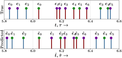
Figure 3. Qualitative Analysis of mark and time prediction performance of IMTPP over the synthetic dataset. In the top figure, we show the observed (bars in blue) as well as events hidden (bars in brown) during learning between timestamps $6.0$ and $6.4$. In the lower figure, we show the events predicted by IMTPP for the same sequence. Marks are represented using different colored (cyan and purple) circles.

6.3. Prediction of Missing Events (RQ1)

To address the research question RQ1, we first qualitatively demonstrate the ability of IMTPP in predicting missing events in sequences from the synthetic dataset. To do so, we randomly sample 10% events from each sequence and tag them to be missing. Later, we train IMTPP over the observed events and use our trained model to predict both observed and missing events. Figure 3 provides an illustrative setting of our results. It shows that IMTPP provides many accurate mark predictions. In addition, it qualitatively shows that the predicted inter-arrival times and marks closely match with the true inter-arrival times. Thus supporting the ability of IMTPP to accurately identify the marks and times of missing events as well as the total number of events missing between two timestamps. Note that we utilize synthetic deletion only for the results in Figure 3 and for other results in the paper, we use complete sequences unless mentioned specifically.

6.4. Event Prediction Performance (RQ2)

Next, we evaluate the event prediction ability of IMTPP. More specifically, we compare the performance of IMTPP with all the baselines introduced above across all six datasets. Tables 3 and 3 summarizes the results, which sketches the comparative analysis in terms of mean absolute error (MAE) on time and mark prediction accuracy (MPA), respectively. From the results we make the following observations:

1. IMTPP exhibits steady improvement over all the baselines in most of the datasets, in case of both time and mark prediction. However, for Stackoverflow and Foursquare datasets, THP outperforms all other models including IMTPP in terms of MPA.

2. RMTPP is the second-best performer in terms of MAE of time prediction almost in all datasets. In fact, in Stackoverflow (SO) dataset, it shares the lowest MAE together with IMTPP. However, there is no consistent second-best performer in terms of MPA. Notably, PFPP and IMTPP, which take into account missing events, are the second-best performers for four datasets.

3. Both PFPP (Mei et al., 2019) and HPMD (Shelton et al., 2018) fare poorly with respect to IMTPP in terms of both MAE and MPA. This is because PFPP focuses on imputing missing events based on the complete observations and, is not well suited to predict observed events in the face of missing observations. In fact, PFPP does not offer a joint training mechanism for the MTPP for observed events and the imputation model. Rather it trains an imputation model based on the observation model learned a-priori. On the other hand, HPMD only assumes a linear Hawkes process with a known influence structure. Therefore it shows poor performance with respect to IMTPP.

Table 2. Performance of all the methods in terms of mean absolute error across all datasets on the 20% test set. Numbers with bold font (boxes) indicate best (second best) performer. Results marked ^$\dagger$ are statistically significant (two-sided Fisher’s test with $p\leq 0.1$) over the best baseline.

Dataset	Mean Absolute Error (MAE)
	Movies	Toys	Taxi	Twitter	SO	Foursquare	Celebrity	Health
HP (Hawkes, 1971)	0.060	0.062	0.220	0.049	0.010	0.098	0.044	0.023
SMHP (Liniger, 2009)	0.062	0.061	0.213	0.051	0.008	0.091	0.043	0.024
RMTPP (Du et al., 2016)	0.053	0.048	0.128	0.040	0.005	0.047	0.036	0.021
SAHP (Zhang et al., 2020)	0.072	0.073	0.174	0.081	0.017	0.108	0.051	0.027
THP (Zuo et al., 2020)	0.068	0.057	0.193	0.047	0.006	0.052	0.040	0.026
PFPP (Mei et al., 2019)	0.058	0.055	0.181	0.042	0.007	0.076	0.039	0.022
HPMD (Shelton et al., 2018)	0.060	0.061	0.208	0.048	0.008	0.087	0.043	0.023
IMTPP	0.049$\dagger$	0.045$\dagger$	0.108$\dagger$	0.038$\dagger$	0.005	0.041$\dagger$	0.032$\dagger$	0.019$\dagger$

Table 3. Performance of all the methods in terms of mark prediction accuracy (MPA). Numbers with bold font (boxes) indicate best (second best) performer. Results marked ^$\dagger$ are statistically significant (two-sided Fisher’s test with $p\leq 0.1$) over the best baseline.

Dataset	Mark Prediction Accuracy (MPA)
	Movies	Toys	Taxi	Twitter	SO	Foursquare	Celebrity	Health
HP (Hawkes, 1971)	0.482	0.685	0.894	0.531	0.418	0.523	0.229	0.405
SMHP (Liniger, 2009)	0.501	0.683	0.893	0.554	0.423	0.520	0.238	0.401
RMTPP (Du et al., 2016)	0.548	0.734	0.929	0.572	0.446	0.605	0.255	0.421
SAHP (Zhang et al., 2020)	0.458	0.602	0.863	0.461	0.343	0.459	0.227	0.353
THP (Zuo et al., 2020)	0.537	0.724	0.931	0.526	0.458	0.624	0.268	0.425
PFPP (Mei et al., 2019)	0.559	0.738	0.925	0.569	0.437	0.582	0.256	0.427
HPMD (Shelton et al., 2018)	0.513	0.688	0.907	0.558	0.439	0.531	0.247	0.409
IMTPP	0.574$\dagger$	0.746$\dagger$	0.938$\dagger$	0.577	0.451	0.612	0.273	0.438$\dagger$

Qualitative Analysis. In addition, we also perform a qualitative analysis to identify if IMTPP can model the inter-event time-intervals in a sequence. Figure 4 provides some real-life event sequences taken from Movies and Toys datasets and the time-intervals predicted by IMTPP. The results qualitatively show that the predicted inter-arrival times closely match with the true inter-arrival times. Moreover, the results also show that IMTPP can event efficiently model the large spikes in inter-event time-intervals.

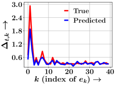
(a) Movies

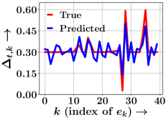
(b) Toys

Figure 4. Real life examples of true and predicted inter-arrival times $\Delta_{t,k}$ of different events $e_{k}$, against $k$ for $k\in\{k+1,\ldots,N\}$. Panels (a) and (b) show the results for Movies and Toys datasets respectively.

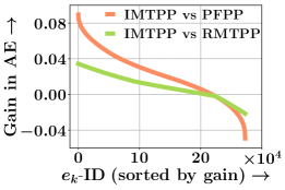
(a) Movies

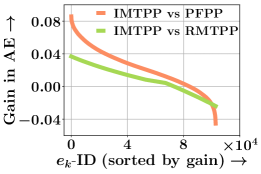
(b) Toys

Figure 5. Performance gain in terms of $\text{AE}(\text{baseline})-\text{AE}(\textsc{IMTPP})$— the gain (above x-axis) or loss (below x-axis) of the average error per event $\mathbb{E}[|t_{k}-\hat{t_{k}}|]$ of IMTPP— with respect to two competitive baselines: RMTPP and PFPP. Events in the test set are sorted by decreasing gain of IMTPP along $x$-axis. Panels (a) and (b) show the results for Movies and Toys datasets respectively.

Drill-down Analysis. Next, we provide a comparative analysis of the time prediction performance at the level of every event in the test set. To this end, for each observed event $e_{i}$ in the test set, we compute the gain (or loss) IMTPP achieves in terms of the time-prediction error per event $\mathbb{E}[|t_{k}-\hat{t_{k}}|]$, i.e., $\text{AE}(\text{baseline})-\text{AE}(\textsc{IMTPP})$ for two competitive baselines, e.g., RMTPP and PFPP for Movies and Toys datasets. Figure 5 summarizes the results, which shows that IMTPP outperforms the most competitive baseline i.e. RMTPP for more than 70% events across both Movies and Toys datasets. It also shows that the performance gain of IMTPP over PFPP is ever more significant.

Table 4. Time prediction performance of IMTPP and its variants – $\textsc{IMTPP}_{\mathcal{S}}$and $\textsc{IMTPP}_{\mathcal{R}}$in terms of MAE on the 20% test set. Numbers with bold font indicate the best performer.

Dataset	Mean Absolute Error (MAE)
	Movies	Toys	Taxi	Twitter	SO	Foursquare	Celebrity	Health
$\textsc{IMTPP}_{\mathcal{S}}$	0.054	0.047	0.115	0.042	0.005	0.044	0.034	0.021
$\textsc{IMTPP}_{\mathcal{R}}$	0.056	0.051	0.120	0.041	0.006	0.043	0.037	0.023
IMTPP	0.049	0.045	0.108	0.038	0.005	0.041	0.032	0.019

Table 5. Mark prediction performance of IMTPP and its variants in terms of MPA on the 20% test set. Numbers with bold font indicate the best performer.

Dataset	Mark Prediction Accuracy (MPA)
	Movies	Toys	Taxi	Twitter	SO	Foursquare	Celebrity	Health
$\textsc{IMTPP}_{\mathcal{S}}$	0.569	0.742	0.929	0.574	0.450	0.603	0.267	0.425
$\textsc{IMTPP}_{\mathcal{R}}$	0.563	0.724	0.927	0.568	0.449	0.598	0.261	0.433
IMTPP	0.574	0.746	0.938	0.577	0.451	0.612	0.273	0.438

6.5. Ablation Study

We also conduct an ablation study for two key contributions in IMTPP: missing event MTPP and the intensity-free modeling of time-intervals. We denote $\textsc{IMTPP}_{\mathcal{S}}$as the variants of IMTPP without the missing MTPP and $\textsc{IMTPP}_{\mathcal{R}}$as the variant without the lognormal distribution for inter-event arrival times. More specifically, for $\textsc{IMTPP}_{\mathcal{R}}$we follow (Du et al., 2016) to determine an intensity function $\lambda^{p}_{k}$ for observed events using the output of the RNN, $\bm{s}_{k}$.

(23) $$\lambda^{*}_{p}(t_{k})=\exp(\bm{w}_{\lambda,s}\bm{s}_{k}+\bm{w}_{\lambda,m}\bm{m}_{\overline{k}}+\bm{w}_{\lambda,\Delta}(t_{k}-t_{k-1})+\bm{b}_{\lambda}),$$

Later, we use the intensity function at a given timestamp to estimate the probability distribution of future events as:

(24) $$p_{\theta,t}(t_{k+1})=\lambda^{*}_{p}(t_{k})\exp\left(-\int_{t_{k}}^{t}\lambda^{*}_{p}(\tau)\,d\tau\right),$$

Similar to RQ2, we report the performance of IMTPP and its variants in terms of MAE and MPA in Tables 5 and 5 respectively. The results show that IMTPP outperforms $\textsc{IMTPP}_{\mathcal{S}}$and $\textsc{IMTPP}_{\mathcal{R}}$across all metrics. The performance gain of IMTPP over $\textsc{IMTPP}_{\mathcal{S}}$signifies the importance of including missing events for modeling event sequences. We also note that the performance gain of IMTPP over $\textsc{IMTPP}_{\mathcal{R}}$reinforces our modeling design of using an intensity-free model for MTPPs.

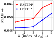
(a) Movies, MAE

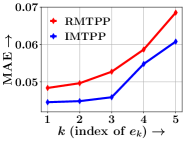
(b) Toys, MAE

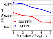
(c) Movies, MPA

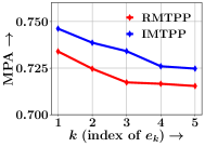
(d) Toys, MPA

Figure 6. Variation of forecasting performance of IMTPP and RMTPP in terms of MAE and MPA at predicting next $i$-th event, against $i$ for Movies and Toys dataset. Panels (a–b) show the variation of MAE while panels (c–d) show the variation of MPA. They show that as $n$ increases, the performance deteriorates for both the metrics and both datasets as the prediction task becomes more and more difficult.

6.6. Forecasting Future Events (RQ3)

To make a more challenging evaluation of IMTPP against its competitors we design a difficult event prediction task, where we predict the next $n$ events given only the current event as input. To do so, we keep sampling events using the trained model $p_{\hat{\theta}}$ and $q_{\hat{\phi}}$ till $n$-th prediction. Such an evaluation protocol effectively requires accurate inference of the missing data distribution, since, unlike during the training phase, the future observations are not fed into the missing event model. To this end, we compare the forecasting performance of IMTPP against RMTPP, the most competitive baseline. Figure 6 summarizes the results for Movies and Toys datasets, which shows that (1) the performances of all the algorithms deteriorate as $n$ increases and; (2 IMTPP achieves  5.5% improvements in MPA and significantly better 10.12% improvements in MAE than RMTPP across both datasets. The results further reinforce the ability of IMTPP to model the long-term distribution of events in a sequence.

Table 6. Mark prediction performance of Markov Chains and IMTPP across all datasets. We use MC of orders 1,2, and 3 and report results for the best performing model.

Dataset	Mark Prediction Accuracy (MPA)
	Movies	Toys	Taxi	Twitter	SO	Foursquare	Celebrity	Health
MC	0.542	0.702	0.829	0.548	0.443	0.575	0.249	0.416
IMTPP	0.574	0.746	0.938	0.577	0.451	0.612	0.273	0.438

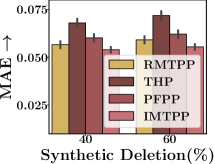
(a) Movies, MAE

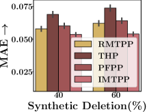
(b) Toys, MAE

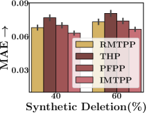
(c) Synthetic, MAE

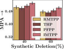
(d) Movies, MPA

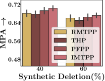
(e) Toys, MPA

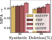
(f) Synthetic, MPA

Figure 7. Impact of missing observations on model performance for Movies, Toys and Synthetic dataset. We randomly delete 40% and 60% events from the observed sequence and then train and test IMTPP and best performing baselines on rest of the observed events. Panels (a–c) show the results for time prediction while panels (d–f) show the results for mark prediction. The performance improvement of IMTPP in such a situation is still significant as in the original setting— without any artificial data deletion.

6.7. Performance Comparison with Markov Chains

Previous research (Du et al., 2016) has shown that the mark prediction performance of neural MTPP models is comparable to Markov Chains (MCs). Therefore, in addition to the mark prediction experiments with MTPP models in Table 3, we also report the results for the comparison between IMTPP and MCs of orders $1$ to $3$ in Table 6. Note that we only report the results of the best-performing MC. The results show that the Markov models perform quite well in terms of mark prediction accuracy across all datasets. A careful investigation revealed that the datasets exhibit significant repetitive characteristics of marks in a small window. Thus for some datasets with large repetitions within a short history window, using a deep point process-based model is an overkill. On the other hand, for NYC Taxi, the mobility distribution clearly shows long-term dependencies, thus severely hampering the performance of Markov Chains. In these cases, point process-based models show better performance by being able to model the inter-event complex dependencies more efficiently.

6.8. Performance with Missing Data

To further emphasize the applicability of IMTPP in the presence of missing data, we perform event prediction on sequences with limited training data. Specifically, we synthetically delete events from a sequence i.e. we randomly (via a normal distribution) delete $40\%$ (and $60\%$) of events from the original sequence and then train and test our model on the rest $60\%$ events($40\%$). Figure 7 summarizes the results across Movies, Toys, and the Synthetic dataset. From the results, we note that with synthetic data deletion, the performance improvement of IMTPP over best-performing baselines – RMTPP, THP and PFPP– is significant event after 40% events are deleted. This is because IMTPP is trained to capture the missing events and as a result, it can exploit the underlying setting with data deletion more effectively than the other models. Though this performance gains saturate with further increase in missing data as the added noise in the datasets severely hampers the learning of both models. Interestingly, we note that RMTPP outperforms THP and PFPP even in the situations with limited data.

6.9. Scalability Analysis (RQ4)

Here we compare the runtime of IMTPP with PFPP (Mei et al., 2019) in two settings: (1) training over complete sequences, and (2) training in a streaming setting.

6.9.1. With Complete Sequences

To highlight the time-effective learning ability of IMTPP, we compare the runtimes of IMTPP and PFPP across no. of training epochs as well as the length of training sequence $|\mathcal{S}_{K}|$. Figure 8 summarizes the results, which shows that IMTPP enjoys a better latency than PFPP. In particular, we observe that the runtime of PFPP increases quadratically with respect to $|\mathcal{S}_{K}|$, whereas, the runtime of IMTPP increases linearly. The quadratic complexity of PFPP is due to the presence of a backward RNN which requires a complete pass whenever a new event arrives. The larger run-times of both models can be attributed to the massive size of Movies dataset with $1.4$ million events.

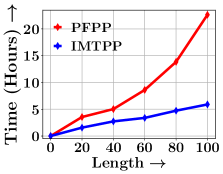
(a) Time vs $|\mathcal{S}_{K}|$

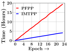
(b) Time vs # of epochs

Figure 8. Runtime performance of PFPP and IMTPP for across Movies dataset with complete sequences. Panel (a) shows time vs. length of training sequence and panel (b) shows time vs. number of epochs.

Table 7. Runtime comparison between IMTPP and PFPP in a streaming setting. Here, DNF indicates that the code did not finish within 24:00hrs.

Dataset	Runtime (Hours)
	Movies	Toys	Taxi	Twitter	SO	Foursquare	Celebrity	Health
IMTPP	<2hr	<2hr	<1hr	<2hr	<1hr	<1hr	<2hr	<2hr
PFPP (Mei et al., 2019)	DNF	DNF	DNF	DNF	DNF	DNF	DNF	DNF

6.9.2. Streaming-based Runtime

As mentioned in Section 4, our setting differs significantly from PFPP (Mei et al., 2019) as it requires the complete data distribution, missing as well as observed, upfront for operating. However, we evaluate if their model can be extended to our setting i.e. a streaming setting wherein complete sequences are not available upfront rather they arrive as we progress with time along a sequence. In a streaming setting, the model is trained as per the arrival of events, and the only way for PFPP to be extended in this setting is to update the parameters at each arrival. This repetitive training is expensive and can withdraw the practicability of the model. To further assert our proposition, we evaluate the runtime of their model across the different datasets and compare with IMTPP. We report the results for training across only a few epochs (10) in a streaming setting in Table 7. We note that across all datasets PFPP fails to scale as expected. This delay in training could be attributed to the two-phase training of their model; (1) particle filtering, where they learn the underlying complete data distribution, and (2) particle smoothing, in which they filter out the inadequate events generated during particle filtering. Secondly, since PFPP requires complete data during training, an online setting would require repetitive parameter optimization on the arrival of each event. Thus, their model cannot be extended to such a scenario while maintaining its practicality. Thus, IMTPP is the singular practical approach for learning MTPPs in an online setting with intermittent observational data.

6.10. Imputation Performance

Here, we evaluate the ability of IMTPP and PFPP to impute missing events in a sequence. Specifically, we evaluate the ability of both models to generate the missing events that were not present during training. Thus, for Movies and Toys datasets where we synthetically remove all the ratings between the first month and the third month for all the entities in both datasets. We evaluate across the imputed events for test sequences. One important thing to note is that IMTPP only takes into account the history, but PFPP uses both, history and future events. We report the results across the Movies and Toys datasets in Figure 9. To summarize, our results show that even with limited historical information, IMTPP outperforms PFPP in time-prediction whereas both models perform competitively for mark prediction of missing events.

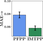
(a) Movies, MAE

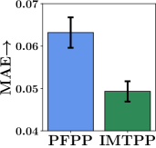
(b) Toys, MAE

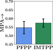
(c) Movies, MPA

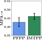
(d) Toys, MPA

Figure 9. Missing event imputation performance of IMTPP and PFPP for Movies and Toys datasets. Panels (a–b) show the results for time prediction while panels (c–d) show the results for mark prediction.

(a) Movies, MAE

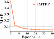
(b) Toys, MAE

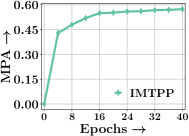
(c) Movies, MPA

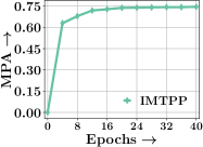
(d) Toys, MPA

Figure 10. Epoch-wise event prediction performance of IMTPP for Movies and Toys datasets. Panels (a–b) show the results for time prediction while panels (c–d) show the results for mark prediction. The results show that IMTPP exhibits a stable optimization procedure. The MAE before the first training epoch is clipped to $0.5$.

6.11. Convergence Analysis

Here, we highlight the stable convergence of the optimization procedure of IMTPP event after modeling the dynamics of observed as well as missing events. Therefore, we plot the epoch-wise best event prediction performance of IMTPP in terms of MAE and MPA in Figure 10. The results show that despite the coupled MTPP model and its variational inference-based learning, IMTPP exhibits stable optimization procedure. We also note that mark prediction performance shows better convergence and outperforms other models only in a few training iterations. However, the time prediction ability of IMTPP requires longer training to achieve state-of-the-art performance.

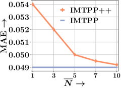
(a) Movies

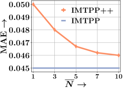
(b) Toys

Figure 11. Predicting observed events using IMTPP++ across different values of $\overline{N}$. The results show that as we increase $\overline{N}$, the performance gap between IMTPP++ and IMTPP is decreased.

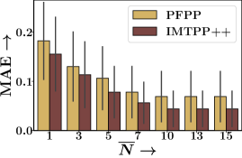
(a) Movies

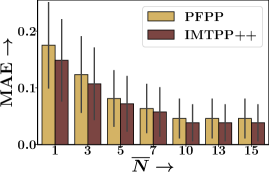
(b) Toys

Figure 12. Compared the imputation performance of IMTPP++ and PFPP across different numbers of missing events. Note that this setting differs from Figure 9, as here the events are missing at random positions.

6.12. Performance of IMTPP++

In this section, we evaluate the performance of IMTPP++ across two settings – (1) predicting future observed events, and (2) imputing missing events.

6.12.1. Observed Event Prediction

Here we evaluate the ability of IMTPP++ to predict the observed events in a sequence. Specifically, we report the time prediction performance of IMTPP++ across a different number of permitted missing events ($\overline{N}$) and compare them with IMTPP i.e. with an unbounded number of missing events. Figure 11 summarizes our results which show that as we increase $\overline{N}$, the time prediction performance for IMTPP++ increases and it narrows the performance gap with IMTPP. However, IMTPP still performs better than IMTPP++. From the results, we conclude that IMTPP++ acts as a trade-off between the number of missing events and the prediction quality. This is a significant improvement over IMTPP as sampling missing events can be an expensive procedure. Moreover, as IMTPP++ involves a fine-tuning over pre-trained IMTPP, it has an added advantage of fine-tuning at amounts of missing events. From our experiments, we found that fine-tuning IMTPP++ took less than 15 minutes across all values of $\overline{N}$. We also note that with small $\overline{N}$, IMTPP is comparable to RMTPP i.e. the best performer for time prediction.

6.12.2. Imputing Missing Events

Our main contribution via IMTPP++ is to predict the missing events located randomly in a sequence. We evaluate this by performing an additional experiment using synthetic deletion. Specifically, we randomly sample $\overline{N}$ events from each sequence and tag them to be missing. Later, we evaluate the ability of IMTPP++ and PFPP in imputing these missing events. Figure 12 summarizes the results and we note that IMTPP++ easily outperforms PFPP across all values of $\overline{N}$. Moreover, we note that as we increase $\overline{N}$, the imputation performance becomes better. Naturally, it can be attributed to relatively lesser variance in position of missing events with large $\overline{N}$. We reiterate that all confidence intervals are calculated using three independent runs.

6.13. Performance Variation with $p_{\text{prior}}$

Here, we train our model with different values of the prior scaling factor ($\bar{\mu}$) and then probe the variation of predictive performance. We highlight that $\bar{\mu}$ differs from the mean of the log-normal flow of prior MTPP, though they share similar notations. To get a deeper insight into the contribution of the prior MTPP and the dataset dynamics, we also experiment with different training set sizes as in Section 6.8. For this evaluation, we consider the Movies dataset across 40% and 60% training data and plot the MPA and MAE against $\bar{\mu}$. Figure 13 summarizes the results and we note that there exist two particular trends corresponding to MAE and MPA across different $\bar{\mu}$. For MAE, as $\bar{\mu}$ increases its first decreases and then increases, whereas, for MPA, it first increases and then decreases. Both the trends indicate the presence of an optimal value of $\bar{\mu}$. This tendency of IMTPP is consistent across different subsets of training data as well. Moreover, we also note that the optimal value for $\bar{\mu}$ also changes as per the size of the training set.

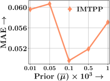
(a) Movies

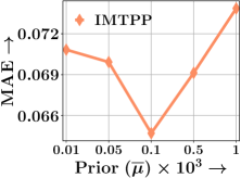
(b) Movies (60%)

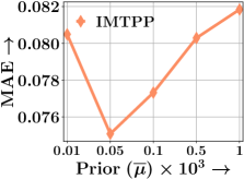
(c) Movies (40%)

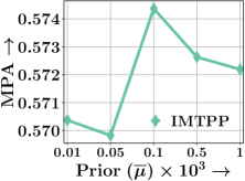
(d) Movies

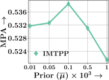
(e) Movies (60%)

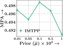
(f) Movies (40%)

Figure 13. Variation of forecasting performance of IMTPP against $\bar{\mu}$, the prior rate of missing events, for Movies dataset. Panels (a–c) show the variation of MAE while panels (d–f) show the variation of MPA. As $\bar{\mu}$ increases MAE first decreases and then increases, indicating the presence of an optimal $\bar{\mu}$ across training data sizes. The results for MPA against $\bar{\mu}$ also show the presence of an optimal $\bar{\mu}$ across training data sizes.

7. Conclusion

Modeling continuous-time events with irregular observations is a non-trivial task that requires learning the distribution of both – observed and missing events. Standard MTPP models ignore this aspect and assume that the underlying data is complete with no missing events – an ideal assumption that is not practicable in many settings. In order to solve these shortcomings, in this paper, we provide a method for incorporating missing events for training marked temporal point processes, that simultaneously samples missing as well as observed events across continuous time. The proposed model IMTPP uses a coupled MTPP approach with its parameters optimized via variational inference. Experiments on several real datasets from diverse application domains show that our proposal outperforms other state-of-the-art approaches for predicting the dynamics of observed events. We also evaluate the ability of IMTPP to impute synthetically deleted missing events within observed events. In this setting as well, IMTPP outperforms other alternatives along with better scalability and guaranteed convergence. Since including missing data, improves over standard learning procedures, this observation opens avenues for further research that includes modeling or sampling missing data. However, one unaddressed aspect of the missing data problem is partially missing events i.e. events with either the time or mark as missing. In addition, the constrained optimization procedure in IMTPP++ can be improved by using Lagrangian multipliers. This would prevent the two-step procedure mentioned in Section 5.6 while simultaneously facilitating faster convergence. Therefore, we plan to extend our model for modeling partially missing events and using the enhanced learning procedure for IMTPP++ as future works of this paper.

References

- (1)
- Bacry et al. (2015) Emmanuel Bacry, Iacopo Mastromatteo, and Jean-François Muzy. 2015. Hawkes processes in finance. arXiv preprint arXiv:1502.04592 (2015).
- Bai et al. (2018) Tian Bai, Shanshan Zhang, Brian L. Egleston, and Slobodan Vucetic. 2018. Interpretable Representation Learning for Healthcare via Capturing Disease Progression through Time. In KDD.
- Baim et al. (1986) Donald S. Baim, Wilson S. Colucci, E. Scott Monrad, Harton S. Smith, Richard F. Wright, Alyce Lanoue, Diane F. Gauthier, Bernard J. Ransil, William Grossman, and Eugene Braunwald. 1986. Survival of patients with severe congestive heart failure treated with oral milrinone. Journal of the American College of Cardiology 7, 3 (1986), 661–670.
- Bowman et al. (2015) Samuel R Bowman, Luke Vilnis, Oriol Vinyals, Andrew M Dai, Rafal Jozefowicz, and Samy Bengio. 2015. Generating sentences from a continuous space. arXiv preprint arXiv:1511.06349 (2015).
- Cao et al. (2018) Wei Cao, Dong Wang, Jian Li, Hao Zhou, Lei Li, and Yitan Li. 2018. BRITS: Bidirectional Recurrent Imputation for Time Series. In NeurIPS.
- Che et al. (2016) Zhengping Che, Sanjay Purushotham, Kyunghyun Cho, David Sontag, and Yan Liu. 2016. Recurrent Neural Networks for Multivariate Time Series with Missing Values. arXiv preprint arXiv:1606.01865 (2016).
- Chung et al. (2015) Junyoung Chung, Kyle Kastner, Laurent Dinh, Kratarth Goel, Aaron C Courville, and Yoshua Bengio. 2015. A recurrent latent variable model for sequential data. In NeurIPS.
- Daley and Vere-Jones (2007) Daryl J Daley and David Vere-Jones. 2007. An introduction to the theory of point processes: volume II: general theory and structure. Springer Science & Business Media.
- De et al. (2016) Abir De, Isabel Valera, Niloy Ganguly, Sourangshu Bhattacharya, and Manuel Gomez-Rodriguez. 2016. Learning and Forecasting Opinion Dynamics in Social Networks. In NeurIPS.
- Deshpande et al. (2021) Prathamesh Deshpande, Kamlesh Marathe, Abir De, and Sunita Sarawagi. 2021. Long Horizon Forecasting With Temporal Point Processes. In WSDM.
- Doersch (2016) Carl Doersch. 2016. Tutorial on variational autoencoders. arXiv preprint arXiv:1606.05908 (2016).
- Du et al. (2016) Nan Du, Hanjun Dai, Rakshit Trivedi, Utkarsh Upadhyay, Manuel Gomez-Rodriguez, and Le Song. 2016. Recurrent marked temporal point processes: Embedding event history to vector. In KDD.
- Du et al. (2015) Nan Du, Mehrdad Farajtabar, Amr Ahmed, Alexander J Smola, and Le Song. 2015. Dirichlet-hawkes processes with applications to clustering continuous-time document streams. In KDD.
- Farajtabar et al. (2017) Mehrdad Farajtabar, Jiachen Yang, Xiaojing Ye, Huan Xu, Rakshit Trivedi, Elias Khalil, Shuang Li, Le Song, and Hongyuan Zha. 2017. Fake news mitigation via point process based intervention. In ICML.
- Ghazi et al. (2019) Mostafa Mehdipour Ghazi, Mads Nielsen, Akshay Pai, M Jorge Cardoso, Marc Modat, Sébastien Ourselin, and Lauge Sørensen. 2019. Training recurrent neural networks robust to incomplete data: application to Alzheimer’s disease progression modeling. Medical image analysis 53 (2019), 39–46.
- Guo et al. (2018) Ruocheng Guo, Jundong Li, and Huan Liu. 2018. INITIATOR: Noise-contrastive Estimation for Marked Temporal Point Process. In IJCAI.
- Gupta and Bedathur (2021) Vinayak Gupta and Srikanta Bedathur. 2021. Region Invariant Normalizing Flows for Mobility Transfer. In CIKM.
- Gupta and Bedathur (2022a) Vinayak Gupta and Srikanta Bedathur. 2022a. Doing More with Less: Overcoming Data Scarcity for POI Recommendation via Cross-Region Transfer. arXiv preprint arXiv:2201.06095 (2022).
- Gupta and Bedathur (2022b) Vinayak Gupta and Srikanta Bedathur. 2022b. ProActive: Self-Attentive Temporal Point Process Flows for Activity Sequences. arXiv preprint arXiv:2206.05291 (2022).
- Gupta et al. (2021) Vinayak Gupta, Srikanta Bedathur, Sourangshu Bhattacharya, and Abir De. 2021. Learning Temporal Point Processes with Intermittent Observations. In AISTATS.
- Gupta et al. (2022) Vinayak Gupta, Srikanta Bedathur, and Abir De. 2022. Learning Temporal Point Processes for Efficient Retrieval of Continuous Time Event Sequences. In AAAI.
- Hawkes (1971) Alan G Hawkes. 1971. Spectra of some self-exciting and mutually exciting point processes. Biometrika 58, 1 (1971), 83–90.
- Huang et al. (2019) Hengguang Huang, Hao Wang, and Brian Mak. 2019. Recurrent poisson process unit for speech recognition. In AAAI.
- Jing and Smola (2017) How Jing and Alexander J Smola. 2017. Neural survival recommender. In WSDM.
- Kumar et al. (2019) Srijan Kumar, Xikun Zhang, and Jure Leskovec. 2019. Predicting dynamic embedding trajectory in temporal interaction networks. In KDD.
- Li et al. (2018a) Shuang Li, Shuai Xiao, Shixiang Zhu, Nan Du, Yao Xie, and Le Song. 2018a. Learning Temporal Point Processes via Reinforcement Learning. In NeurIPS.
- Li et al. (2018b) Youru Li, Zhenfeng Zhu, Deqiang Kong, Hua Han, and Yao Zhao. 2018b. EA-LSTM: Evolutionary Attention-based LSTM for Time Series Prediction. arXiv preprint arXiv:1811.03760 (2018).
- Likhyani et al. (2020) Ankita Likhyani, Vinayak Gupta, PK Srijith, P Deepak, and Srikanta Bedathur. 2020. Modeling Implicit Communities from Geo-tagged Event Traces using Spatio-Temporal Point Processes. In WISE.
- Liniger (2009) Thomas Josef Liniger. 2009. Multivariate hawkes processes. Ph.D. Dissertation. ETH Zurich.
- Little and Rubin (2019) Roderick JA Little and Donald B Rubin. 2019. Statistical analysis with missing data. John Wiley & Sons.
- Lorch et al. (2018) Lars Lorch, Abir De, Samir Bhatt, William Trouleau, Utkarsh Upadhyay, and Manuel Gomez-Rodriguez. 2018. Stochastic Optimal Control of Epidemic Processes in Networks. arXiv preprint arXiv:1810.13043 (2018).
- Luo et al. (2018) Yonghong Luo, Xiangrui Cai, Ying Zhang, Jun Xu, and Yuan Xiaojie. 2018. Multivariate Time Series Imputation with Generative Adversarial Networks. In NeurIPS.
- Luo et al. (2019) Yonghong Luo, Ying Zhang, Xiangrui Cai, and Xiaojie Yuan. 2019. E²GAN: End-to-End Generative Adversarial Network for Multivariate Time Series Imputation. In IJCAI.
- Mehrasa et al. (2019) Nazanin Mehrasa, Akash Abdu Jyothi, Thibaut Durand, Jiawei He, Leonid Sigal, and Greg Mori. 2019. A Variational Auto-Encoder Model for Stochastic Point Processes. In CVPR.
- Mei and Eisner (2017) Hongyuan Mei and Jason M Eisner. 2017. The neural hawkes process: A neurally self-modulating multivariate point process. In NeurIPS.
- Mei et al. (2019) Hongyuan Mei, Guanghui Qin, and Jason Eisner. 2019. Imputing Missing Events in Continuous-Time Event Streams. In ICML.
- Mueen and Keogh (2016) Abdullah Mueen and Eamonn Keogh. 2016. Extracting optimal performance from dynamic time warping. In KDD.
- Nagrani et al. (2017) A. Nagrani, J. S. Chung, and A. Zisserman. 2017. VoxCeleb: a large-scale speaker identification dataset. In INTERSPEECH.
- Ni et al. (2019) Jianmo Ni, Jiacheng Li, and Julian McAuley. 2019. Justifying recommendations using distantly-labeled reviews and fine-grained aspects. In EMNLP-IJCNLP.
- Omi et al. (2019) Takahiro Omi, Naonori Ueda, and Kazuyuki Aihara. 2019. Fully Neural Network based Model for General Temporal Point Processes. In NeurIPS.
- Rakthanmanon et al. (2012) Thanawin Rakthanmanon, Bilson Campana, Abdullah Mueen, Gustavo Batista, Brandon Westover, Qiang Zhu, Jesin Zakaria, and Eamonn Keogh. 2012. Searching and Mining Trillions of Time Series Subsequences under Dynamic Time Warping. In KDD.
- Rasmussen (2013) Jakob Gulddahl Rasmussen. 2013. Bayesian inference for Hawkes processes. Methodology and Computing in Applied Probability 15, 3 (2013), 623–642.
- Rizoiu et al. (2018) Marian-Andrei Rizoiu, Swapnil Mishra, Quyu Kong, Mark Carman, and Lexing Xie. 2018. SIR-Hawkes: on the Relationship Between Epidemic Models and Hawkes Point Processes. In WWW.
- Rizoiu et al. (2017) Marian-Andrei Rizoiu, Lexing Xie, Scott Sanner, Manuel Cebrian, Honglin Yu, and Pascal Van Hentenryck. 2017. Expecting to be hip: Hawkes intensity processes for social media popularity. In WWW.
- Rumelhart et al. (1986) David E Rumelhart, Geoffrey E Hinton, and Ronald J Williams. 1986. Learning representations by back-propagating errors. Nature 323, 6088 (1986), 533–536.
- Shchur et al. (2020) Oleksandr Shchur, Marin Biloš, and Stephan Günnemann. 2020. Intensity-Free Learning of Temporal Point Processes. In ICLR.
- Shelton et al. (2018) Christian R. Shelton, Zhen Qin, and Chandini Shetty. 2018. Hawkes Process Inference with Missing Data. In AAAI.
- Shieh and Keogh (2008) Jin Shieh and Eamonn Keogh. 2008. ISAX: Indexing and Mining Terabyte Sized Time Series. In KDD.
- Smieja et al. (2018) Marek Smieja, Lukasz Struski, Jacek Tabor, Bartosz Zielinski, and Przemyslaw Spurek. 2018. Processing of Missing Data by Neural Networks. In NeurIPS.
- Tabibian et al. (2019) Behzad Tabibian, Utkarsh Upadhyay, Abir De, Ali Zarezade, Bernhard Schölkopf, and Manuel Gomez-Rodriguez. 2019. Enhancing human learning via spaced repetition optimization. Proceedings of the National Academy of Sciences 116, 10 (2019), 3988–3993.
- Tian et al. (2018) Yan Tian, Kaili Zhang, Jianyuan Li, Xianxuan Lin, and Bailin Yang. 2018. LSTM-based traffic flow prediction with missing data. Neurocomputing 318 (2018), 297–305.
- Valera et al. (2014) Isabel Valera, Manuel Gomez-Rodriguez, and Krishna Gummadi. 2014. Modeling Diffusion of Competing Products and Conventions in Social Media. arXiv preprint arXiv:1406.0516 (2014).
- Vaswani et al. (2017) Ashish Vaswani, Noam Shazeer, Niki Parmar, Jakob Uszkoreit, Llion Jones, Aidan N Gomez, Ł ukasz Kaiser, and Illia Polosukhin. 2017. Attention is All you Need. In NeurIPS.
- Wang et al. (2017) Pengfei Wang, Yanjie Fu, Guannan Liu, Wenqing Hu, and Charu Aggarwal. 2017. Human Mobility Synchronization and Trip Purpose Detection with Mixture of Hawkes Processes. In KDD.
- Wu et al. (2020) Xian Wu, Stephen Mattingly, Shayan Mirjafari, Chao Huang, and Nitesh V Chawla. 2020. Personalized Imputation on Wearable-Sensory Time Series via Knowledge Transfer. In CIKM.
- Wu et al. (2018) Xian Wu, Baoxu Shi, Yuxiao Dong, Chao Huang, Louis Faust, and Nitesh V Chawla. 2018. Restful: Resolution-aware forecasting of behavioral time series data. In CIKM.
- Xiao et al. (2017a) Shuai Xiao, Mehrdad Farajtabar, Xiaojing Ye, Junchi Yan, Le Song, and Hongyuan Zha. 2017a. Wasserstein Learning of Deep Generative Point Process Models. In NeurIPS.
- Xiao et al. (2018) Shuai Xiao, Hongteng Xu, Junchi Yan, Mehrdad Farajtabar, Xiaokang Yang, Le Song, and Hongyuan Zha. 2018. Learning Conditional Generative Models for Temporal Point Processes. In AAAI.
- Xiao et al. (2017b) Shuai Xiao, Junchi Yan, Stephen Chu, Xiaokang Yang, and Hongyuan Zha. 2017b. Modeling the Intensity function of Point Process via Recurrent Neural Networks. In AAAI.
- Xu et al. (2017) Hongteng Xu, Dixin Luo, and Hongyuan Zha. 2017. Learning Hawkes processes from short doubly-censored event sequences. In ICML.
- Yang et al. (2019) Dingqi Yang, Bingqing Qu, Jie Yang, and Philippe Cudre-Mauroux. 2019. Revisiting User Mobility and Social Relationships in LBSNs: A Hypergraph Embedding Approach. In WWW.
- Yoon et al. (2018) Jinsung Yoon, William R Zame, and Mihaela van der Schaar. 2018. Estimating missing data in temporal data streams using multi-directional recurrent neural networks. IEEE Transactions on Biomedical Engineering 66, 5 (2018), 1477–1490.
- Zhang et al. (2020) Qiang Zhang, Aldo Lipani, Omer Kirnap, and Emine Yilmaz. 2020. Self-attentive Hawkes processes. In ICML.
- Zhao et al. (2015) Qingyuan Zhao, Murat A Erdogdu, Hera Y He, Anand Rajaraman, and Jure Leskovec. 2015. Seismic: A self-exciting point process model for predicting tweet popularity. In KDD.
- Zhuang et al. (2020) Jiancang Zhuang, Ting Wang, and Koji Kiyosugi. 2020. Detection and replenishment of missing data in marked point processes. Statistica Sinica 30, 4 (2020), 2105–2130.
- Zuo et al. (2020) Simiao Zuo, Haoming Jiang, Zichong Li, Tuo Zhao, and Hongyuan Zha. 2020. Transformer Hawkes Process. In ICML.