A Novel Multi-Agent Scheduling Mechanism for Adaptation of Production Plans in Case of Supply Chain Disruptions

Abstract

Manufacturing companies typically use sophisticated production planning systems optimizing production steps, often delivering near-optimal solutions. As a downside for delivering a near-optimal schedule, planning systems have high computational demands resulting in hours of computation. Under normal circumstances this is not issue if there is enough buffer time before implementation of the schedule (e.g. at night for the next day). However, in case of unexpected disruptions such as delayed part deliveries or defectively manufactured goods, the planned schedule may become invalid and swift replanning becomes necessary. Such immediate replanning is unsuited for existing optimal planners due to the computational requirements. This paper proposes a novel solution that can effectively and efficiently perform replanning in case of different types of disruptions using an existing plan. The approach is based on the idea to adhere to the existing schedule as much as possible, adapting it based on limited local changes. For that purpose an agent-based scheduling mechanism has been devised, in which agents represent materials and production sites and use local optimization techniques and negotiations to generate an adapted (sufficient, but non-optimal) schedule. The approach has been evaluated using real production data from Huawei, showing that efficient schedules are produced in short time. The system has been implemented as proof of concept and is currently reimplemented and transferred to a production system based on the Jadex agent platform.

[A]J.Jing Tanlabel=e1]jingtan@huawei.com Corresponding author. . [B]L.Lars Braubachlabel=e2]lars.braubach@hs-bremen.de Corresponding author. . [C]K.Kai Janderlabel=e3]jander@th-brandenburg.de Corresponding author. . [D]R.Rongjun Xulabel=e4]xurongjun@huawei.com [E]K.Kai Chenlabel=e5]colin.chenkai@huawei.com

1 Introduction

Companies who have experienced severe supply chain disruptions often report substantial revenue losses and reduced market value after the event [1][2]. Hendricks et al. [3] show that such disruptions are likely to have long-term financial impact.

Mitigation and contingency tactics range from passive acceptance to active customer demand steering [2]. A company’s decision is often an attempt at balancing multiple objectives, when critical decision factors are unclear and causal effects are hard to explain. Vakharia et al. [4] introduces various MIP (Mixed-Integer Programming) models, analytically solving for important decision points such as lead time and safety stock [5], preventive supply chain partner selection [6], optimized material flow (order volume and source) with reliability/robustness constraints [7] and a global supply chain network design [8]. Due to growing complexity in a global supply network, traditional optimization models rely on expert knowledge regarding critical factors in the model as well as the fine-tuning required to overcome potentially huge result variations.

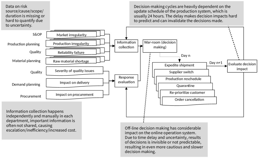
Figure 1: Current process at Huawei to compensate for supply chain disruptions

This study is based on a project of the supply chain department of Huawei Technologies Co. Ltd, an international manufacturing company. Huawei manufactures a large number of complex products which in turn consist of many subcomponents. The subcomponents themselves can either be purchased from a supplier but are also themselves manufactured by Huawei out of even simpler parts. Each of the subcomponents require different inputs and manufacturing processes, resulting in a complex supply chain for each of the final products being manufactured. The supply chain includes multiple suppliers, production facilities and associated logistics to ensure that components are available when they are needed and orders can be fulfilled. However, this complexity also results in the supply chain being vulnerable to disruptions: For example, suppliers may suddenly be unable to deliver components, logistical issues may delay or prevent components from arriving, unexpected breakdowns at manufacturing facilities result in delays or require other facilities to substitute for the failed one.

In addition, some problems may not be immediately apparent: Components may not reach the mandated level of quality or be produced with flaws that are not immediately discovered. When the flaws become apparent, a production batch that has already been produced may have to be quarantined to prevent the flaw from causing quality issues in products down the supply chain. This quarantine leads to an immediate supply shortage that needs to be compensated.

Furthermore, all production batches of both final and intermediate products have production deadlines, the deadlines of intermediate products being driven by the ones of the final products. Simply delaying the delivery of a production batch may result in contractual fines or outright rejection of the production batch by the customer, resulting in financial losses. These deadlines create an urgency in case of suddent disruption of the supply chain that require immediate action to avoid those financial losses.

Since the normal production planning cycle is 24 hours, which may take too long, manual processes are often used to develop steps to compensate the disruption such scenarios. Figure 1 shows the current manual approach used by Huawei in case of unexpected supply chain disruptions: In case of a disruption, a so-called “war room” of experts is created with the aim of finding an immediate solution adjusting the production plans to compensate for the supply shortage caused by the disruption: First, the war room collects all available information. This process step is already impeded by manual information collection and outright missing information about current production runs and schedules. This information often has to be collected manually right from the production facility shop floor.

Once acquired, the war room decision makers use the information to propose changes to the production schedule, for example quickly setting up an extra production run at a different facility. However, such schedule changes in complex supply chains like this are likely to cause ripple effects: The newly-tasked facility is now unavaible for other production runs and may have to delay runs that have already been scheduled. As a result, when the changes are then fed into the standard production planning system, which then takes the changes into account within the next planning cycle, it will show the impact of the changes implemented by the war room on the global supply chain. The war room can then use this information to yet again implement further changes, creating a feedback loop.

Due to ripple effects, many war room actions may be required, however, due to the large feedback delay of 24 hours, the process very cumbersome and difficult, with the impact of changes only visible after a substantial delay. This leads to the results of war room decisions being hard to predict and the decision makers often becoming overly cautious when deciding on necessary scheduling changes. This means that they are often unable to implement bold changes to “save” a production order or are only gradually closing in on a solution over a long time using the feedback loop.

The company was subject to several supply chain disruptions in the past year. "War rooms" were used during such disruptions to share information across functional departments, agree on decisions based on the status quo, wait until the next day for decision effects to materialize and incorporate new inputs to devise further decisions. This iterative process is manual, inefficient and cumbersome to the point of delaying critical decisions.

The goal of this study is not to design a system replacing existing planning and scheduling systems, but instead offers a mechanism, which closely resembles the behavior of such systems, imitating their response at a fraction of the original time at the expense of a slightly reduced solution quality. Typically the standard scheduling system requires hours to reach an optimal solution. If used for simulating various scenarios, it may necessitate days to collect and compare results. This study prototypes a simulation system which enables 1) playing through scenarios in minutes, eliciting responses similar to the actual system supporting urgent management decisions in emergency situations and 2) simulating a diverse set of disruptions of varying severity in advance supporting preventive supply chain design changes.

The study proposes a hybrid approach, solving multiple simple MIP problems in parallel using decentralized multi-agent system. Each agent controls its own resources and is responsible for its own individual and independent objectives. In addition, its visibility is limited to its immediate suppliers and customers (neighboring agents). During disruptions, directly affected agents will start optimizing their individual objectives with simple MIP techniques based on reduced resources (capacity or material); resulting interim results will propagate along the chain to their suppliers or customers in stages aiming to minimize number of nodes which need to deviate from the initial state. In case of conflicts, i.e. a proposal cannot meet the agent’s internal constraints, the agent will optimize and propose an alternative solution, then propagate it back through the chain. The system achieves stability when all agents meet their constraints. Since MIP optimization independently occurs inside each agent, the number of parameters and constraints are substantially reduced compared to modeling and optimizing the entire system. Despite increased communication complexity, the distributed system rapidly stabilizes.

This paper is an extended version of an IDC symposium paper [9] and especially adds background information about the Huawei use case scenario and explains the system realization. It is structured as follows: Section 2 provides a brief overview of current simulation methods. Section 3 describes the system prototype developed in the project. In Section 4 the implementation is outlined. Thereafter, in Section 5 simulation results with sample data are provided. Finally, in Section 5, conclusions are drawn and further research areas are suggested.

2 Related Work

This section presents a broad overview of simulation techniques and agent-based approaches in the context of scheduling problems.

2.1 Simulation Techniques

A common dynamic modeling technique is systems dynamics modeling (SD). As described by Li et al. [10], the modeling approach adjusted by supply chain risk modeling highlights causal inter-dependencies and interactions. Uncertainty is captured through probability distribution of parameters; causal relation (including time delays) is expressed by mathematical equations. Using sampled parameter values and running a Monte-Carlo simulation, worst-, average- and best-case scenarios can be derived. Although suitable for capturing interactions, SD depends on expert knowledge of system structure and parameters [11][12].

Discrete event simulation (DES) is another prevailing modeling technique in logistics and supply chain management. In contrast to SD, it models state changes in discrete time steps and entities are represented individually. In literature review by Tako et al. [13], both simulation techniques are compared. In conclusion, despite both approaches being used extensively as decision support tools, DES is more suitable for operational/tactical level modeling such as local production decisions, whereas SD is more appropriate for long-term and strategic modeling. Choice of modeling technique relies on balancing data volume and complexity of the system structure: in general, a DES system structure requires less expert knowledge while SD requires less data.

2.2 Agent-Based Modeling

Compared to SD or DES, agent-based simulation relies on bottom up modeling of supply chain roles by heterogeneous agents acting autonomously, often using simple rules but expressing behaviors as a system not explicitly programmed (emergent behavior) [14]. A common way of designing agents uses different roles and functionalities in the supply chain. For example, Ledwoch et al. [15] model supply chains with supplier agents, OEM agents and logistic provider agents; Otto et al. [16] employ a similar approach to model response dynamics of a system under production shocks. Such models generally focus on studying complex supply network topology, material and information flow but are deficient modeling operation-level planning and scheduling. They simplify product hierarchy with one or a few dummy products, and rely on general assumptions like time delay to imitate planning processes and capacity limits within each agent. Seck et al. [17] apply a more operative approach to separate agents into product, demand, production, stock, order and batch entities. This approach allows studying networks with more operational aspects such as Bill-Of-Materials (BOM), forecast and firm demands, capacity and optimal production batches, etc. Although tested with a limited number of nodes and products, its model is extensible for more intricate product hierarchies.

Current level of modeling detail in existing approaches is insufficient for daily operational planning and scheduling. These approaches are inadequate for short-term supply chain disruption simulations of individual material codes and production capacity, especially when decisions involve more than 10,000 material codes and hundreds of production lines in various manufacturing locations. Our approach uses agent-based modeling and simulation techniques in which agents are modeled on an even lower level than Seck et al. [17]. Here, each agent represents one specific type of product or production capability. Scheduling of competing products for limited material availability and production capability is done using iterative communication and compromises between agents.

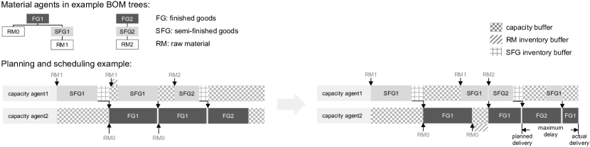
Figure 2: An illustration of rescheduling

Since this study is focused on disruptions, communication and compromise always leads to reduced or delayed production compared to the baseline.

The underlying idea of the approach proposed in this paper consists in having agents that represent important parts of the system with their individual world view and goals. These agents use negotiations to achieve their individual goals and efficiently generate schedules that modify an existing solution. Due to the more limited local data sets, this kind of scheduling in unable to achieve better solutions compared to the optimized quality of results of a global planner. Nevertheless, it is possible to achieve other quality criteria such as high performance (due to more limited local problem spaces and parallelism), any-time solutions (using iterative improvement), few changes to an existing schedule etc. In this respect the approach proposed in this paper shares some similarities with an agent-based hospital logistics simulation approach and system originally developed by some of the authors as part of previous works called MedPAge (medical path agents) [18]. This approach is similar to the proposed system in that it contains agents providing resources (i.e. hospital services) to agents requiring those resources (patients). It also shares a negotiation-based approach towards finding a solution: In this scenario patients and hospital resources like an X-ray machine are represented as agents, while the first group intents to improve their health state as fast as possible and reduce stay time, the latter group prefers to have high utilization of hospital resources. Both types of agents negotiate with each other for appointment and treatment times and can further optimize an initial schedule into a pareto-optimal solution by exchanging received slots. However, the motivations and goals for the system were different from the current proposal in that organizational structures and practices played a significant role while the current approach is aimed at assisting in swiftly handling sudden production disruptions.

3 Agent-based Disruption Scheduling Approach

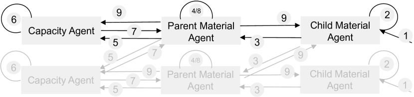
Figure 3: Interaction between agents

The approach is based on real-world Bill-Of-Materials (BOM). A BOM is a tree or network structure representing relationships between raw materials, semi-finished and finished goods. Leaf nodes on the bottom of the tree or network are the lowest-level raw materials and root nodes at the top are finished goods for customers. Material codes on the lower layer need to be produced or purchased before their parent (downstream customer) nodes can be produced. Scheduling complexity can be defined by the number of layers and connections BOMs: BOMs with copious layers and connections imply high levels of inter-dependence between material codes and therefore result in more complex scheduling.

Two types of agents used, representing entities with different capabilities in the supply network. A material agent’s objective is producing a designated type of material in a specific location to satisfy as many of its downstream customer agents’ orders as possible, on time and in full. It has the resources of in-stock and in-transit supply inventory. It controls its own production schedule and has partial visibility into its immediate upstream and downstream agents’ schedules when announcing new proposals concerning its own material. It also includes information of substitute materials for its standard-choice of supply. It can communicate with other agents through a protocol for sending and receiving new scheduling proposals; it can optimize its production schedule or alternatively delay, cancel or combine production orders. It is initialized with a predefined production schedule.

The capacity agent represents the machinery used to produce goods. Like a real-life production line, capacity agents deal with so-called "capacity packages", representing a group of semi-finished or finished goods with similar characteristics so that they can be produced using the same production line in only slightly different configurations. These agents’ objective is to fulfill the maximum number of capacity orders on time and in full. A major difference between a material agent and a capacity agent is that unused capacity left at the end of each planning time unit will be deleted. In case of a resource shortage it can optimize its production and propose new schedules.

Fig. 2 (upper part) demonstrates two simple BOM trees modeled using 7 material agents, 4 of which impose requirements of production capacity on 2 capacity packages (represented by 2 capacity agents). The initial production schedule, as shown in Fig. 2 (lower left part) has built-in inventory and capacity buffers to cope with short-notice schedule changes. Disruption lasting no longer than that buffer length require no rescheduling. If it occurs on short notice lasting for a longer period of time, the planner will attempt rescheduling so that the existing production sequence and amount necessitate minimum change. As an example shown in Fig. 2 (lower left part), the second delivery of RM1 is delayed long enough to affect scheduling of other material codes. Fig. 2 (lower right part) shows one potential rescheduling solution where production of affected SFG1 and FG1 is split.

3.1 Conceptual Overview

Fig. 3 illustrates the interaction between agents based on a single rescheduling iteration. When a disruption occurs, system input data changes to reflect reduced amount of raw materials and/or semi-finished goods. As a first step (cf. 3), this only triggers immediately affected agents. In response, in-stock and in-transit inventory is recalculated. In step 2, triggered agents attempt to reschedule and optimize their production schedules using the new information. The optimization problem is modeled as a simple MIP problem. Due to the agent’s limited visibility and control scope, the potentially complex system-wide optimization problem is reduced to individual agents resolving their own small problems. After solving their own optimization problems, agent propose changes to their downstream customer agents’ schedules. In step 4, the affected customer agents consolidate all change proposals received from their upstream suppliers and optimize their own schedule.

In general, material agent schedules can only degrade under the assumption that supply chain disruption risks always negatively impact the plan. Proposed changes will be propagated to related capacity agents. In steps 5 to 7, communication and rescheduling will be initialized by affected capacity agents. A capacity agent receives change proposals from all relevant material agents and attempts to solve its own optimization problem. Steps 8 and 9 again describe consolidation of new proposals and the corresponding rescheduling activities. The current simulation system only models disruption scenarios. However, it is straightforward to extend to allow simulating human interference such as order priority changes, capacity increases or expedited shipments.

3.2 MIP Problem

Step 2 of the rescheduling iteration includes an optimization problem within the supply material agent (i.e. a child node on a lower level in the BOM) (cf. Section 3.3.1). There are two options used in the simulation: if partial order fulfillment is permitted, agents attempt to produce as early and as much as possible, even if it means full amounts will be produced separately or partially cancelled. If partial order fulfillment is prohibited, agents try to produce orders either in full or not at all. This behavior is modeled after real-world scenarios where customer demands need to be produced and shipped as single batch or completely cancelled by the customer. In step 4, a customer material agent (i.e. a parent node on a higher level in the BOM) solves the optimization problem (cf. Section 3.3.2). It is common source of multiple suppliers who independently delay their material delivery. The plant reschedules its production accommodating all potential delays in one shot instead of dealing with each disruption separately. In step 6, a capacity agent solves its optimization problem (cf. Section 3.4.1). After the system stabilizes, an optional inventory reduction step strips off excessive inventory caused by order cancellation induced by local optimizations in all material agents. This step is not described in detail in this paper.

3.3 Material Agent

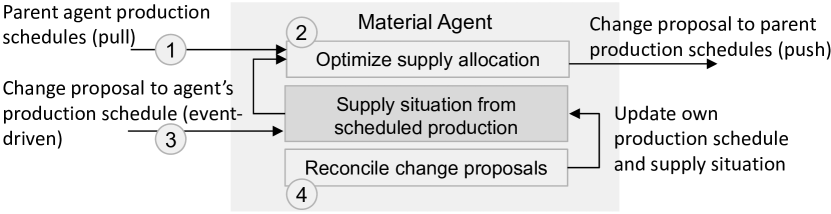
Figure 4: Structure of a material agent

As shown in Fig. 4, the material agent iteratively carries out the following tasks:

1. check planned downstream consumption, update demand-supply situation

2. when production cannot fulfill all demands before required date, try to find best solution by performing optimization from the supplier material agent’s perspective to allocate its available material to each customer

3. event-driven: the agent receives a change request from its upstream supplier agents

4. consolidate all change requests and try to find best solution by performing optimization from the customer material agent’s perspective to reconcile change proposals from its suppliers

5. when all constraints are met, check for potentially excessive inventory and reduce production accordingly

3.3.1 Supplier Material Agent’s Optimization of Schedule

First optimize from a supplier’s perspective: a material agent notices its own produced material quantity cannot fulfill all downstream customer agents’ orders before their demand date. It tries to match as much demand as possible based on the given order priority and the given strategy of order fulfillment: whether it is allowed to fulfill only partial orders.

If partial order fulfillment is allowed, its objective is defined as maximize (using $M$: number of orders; $N$: rescheduling horizon; $d_{mn}$: demand of order m on day n; $s_{n}$: maximum available supply on day n; $x_{mn}$: quantity allocated to order m on day n; $W_{m}$: weight, or priority of order m): $obj=\sum\limits_{m=1}^{M}\sum\limits_{n=1}^{N}W_{m}*x_{mn}$ , with the demand constraints $\sum\limits_{n=1}^{N}x_{mn}<=\sum\limits_{n=1}^{N}d_{mn},\forall m\in[1,M]$ and supply constraints $\sum\limits_{m=1}^{M}x_{mn}<=\sum\limits_{i=1}^{n}s_{i},\forall n\in[1,N]$.

The weight $W_{m}$ is order-priority related. The higher the priority, the higher the weight. It can be linear or nonlinear to priority. The weight used in the project increases linearly with priority.

If orders can only be delivered in full, or be canceled, the agent’s objective is defined as maximize $\sum\limits_{m=1}^{M}\sum\limits_{n=1}^{N}F_{m}*x_{mn}+\sum\limits_{m=1}^{M}\sum\limits_{n=1}^{N}L_{m}*f_{mn}$, where $f_{mn}=x_{mn}*(x_{mn}-d_{mn})$ makes sure the adjusted production quantity is either 0 or the original order quantity. Demand and supply constraints are the same as in the previous problem. $L_{m}$ is the weight of planning adherence. It punishes date changes to the original order and encourages that the existing schedule is kept as much as possible. $F_{m}$ is the weight of order fulfillment. It punishes partially fulfilled orders and encourages orders being produced in full quantity.

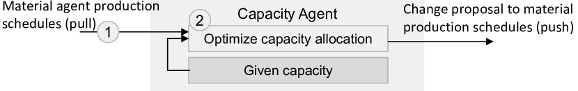
Figure 5: Structure of a capacity agent

3.3.2 Customer Material Agent’s Consolidation of Proposals

From the customer’s perspective a material agent receives multiple schedule change requests from its upstream supplier agents. This is typical in real-world settings where, for example, a logistic disruption result in multiple suppliers delaying delivery, although impact varies based inventory level and severity of disruption. To avoid unnecessarily expediting incoming materials (e.g. since production is already delayed due to other parts from additional suppliers are missing), customer agents should reschedule based on minimum availability.

The agent’s objective is to minimize (using $M$: number of orders; $N$: rescheduling horizon; $q_{mn}$: requested quantity reduction or reschedule of order m on day n; $r_{mn}$: reduced or rescheduled quantity of order m on day n; $W_{mn}$: weight of order m on day n): $obj=\sum\limits_{n=1}^{N}W_{mn}r_{mn}$ with the constraints $\sum\limits_{i=1}^{n}r_{i}>=\sum\limits_{i=1}^{n}q_{mi},\forall m\in[1,M],n\in[1,N]$. The constraints ensure that at any time step the customer agent’s accumulated reduced production quantity is greater than or equal to the proposed reduction quantity from any one of the supplier agents. $W_{mn}$ attenuates later orders and encourages solutions which schedule production as early as possible.

3.4 Capacity Agent

As shown in Fig. 5, the capacity agent iteratively carries out the following tasks:

1. Check planned downstream consumption, update demand-supply situation

2. If capacity cannot fulfill demand, optimize and propose changes to its downstream agents

3.4.1 Capacity Agent’s Consolidation of Proposals

For a capacity agent, the optimization problem has the objective of maximizing (using $M$: number of orders; $N$: rescheduling horizon; $d_{mn}$: demand of order m on day n; $s_{n}$: maximum capacity on day n; $x_{mn}$: quantity allocated to order m on day n): $obj=\sum\limits_{m=1}^{M}\sum\limits_{n=1}^{N}x_{mn},$ with the maximum demand constraints $\sum\limits_{n=1}^{N}x_{mn}<=\sum\limits_{n=1}^{N}d_{mn},\forall m\in[1,M]$ and maximum capacity constraints $\sum\limits_{m=1}^{M}x_{mn}<=s_{n},\forall n\in[1,N]$.

4 Implementation

The simulation system has been implemented using the Jadex Active Components framework [19]. Jadex allows for implementing distributed agent systems using an overlay network of agent platforms, that automatically discover each other depending on virtual network settings [20]. In case of scenarios with deep and complex BOMs, this allows for horizontal scaling by adding platforms according to the needed number of agents. An application built with Jadex can be executed in a local and distributed setup without requiring code modifications as communication between agents is done via remote service interfaces. The agent implementation in Jadex can be done following different agent architectures, i.e. BDI (belief-desire-intention) [21] or simple task-based agents. In any case agents are realized using the unmodified Java programming language so that well-known IDEs like Eclipse can further be used.

The implementation uses a main program that reads Huawei BOM data and creates material and capacity agents accordingly. The material agents will be linked to each other so that each agent knows their parent and child agents. Similarly, material and capacity agents are connected when a production relationship between them exists. Once the setup is completed, the system offers a user interface to initiate different disruption events. To realize the interactions between the agents a service oriented approach has been used, i.e. each agent offers a service that allows for interacting with other agents. In this case, for each agent type one service - called IMaterialService and ICapabilityService - was devised.

⬇

@Service

public interface IMaterialService {

public IFuture<SupplyData> getSupply();

public IFuture<DemandData> getDemand();

public IFuture<Void> addSupply(SupplyData d);

public IFuture<Void> removeSupply(SupplyData d);

public IFuture<Void> addDemand(DemandData d);

public IFuture<Void> removeDemand(DemandData d);

public IFuture<Void> handleChangeProposal(ChangeProposal p);

public IFuture<Schedule> optimizeLocalSchedule();

public IFuture<SupplyData> getSupplyGap();

public IFuture<Void> applyDisruption(DisruptionEvent e);

}

Figure 6: Jadex material service interface

In Fig. 6 the IMaterialService is depicted. It can be seen that the service interface starts with a @Service annotation, which is a marker interface for Jadex that the definition is a remotely callable service. It can also be observed that all methods are declared asynchronously using an IFuture return value. This means that the caller and callee agent are decoupled and the caller will not block until the return value arrives. The real return types are visible as generic types in the future declarations. The interface allows for fetching the current state of the local tasks using getSupply() and getDemand() methods. Furthermore, the state can be changed by adding or removing supply and demand using the following methods. In case another agents intends to influence the internal planning state of the agent, it can do so by calling the handleChangeProposal() method.

Even though in the current prototype, material agents optimize their local schedule only when triggered internally, the service also has a optimizeLocalSchedule() method, which allows for other agents or the user interface to initiate a local replanning. Finally, the supply gap can be fetched and disruption events can be dispatched to the agent. Receiving such an event, the agent will start handling this kind of disruption by internally optimizing and escalating to other agents as far as necessary.

In Fig. 7 the ICapabilityService is depicted. It allows for adding and removing production task using the corresponding add/removeProductionTask methods. In addition the local production schedule at the production site can be obtained using getSchedule(). Similar as in material service, also the capability service offers a method to initiate the local optimization of the capability via optimizeLocalSchedule(). Finally, also the capability service accepts disruption events using applyDisruptionEvent() so that disruption scenarios at a concrete production site can be imitated.

⬇

@Service

public interface ICapacityService {

public IFuture<Void> addProductionTask(ProductionTask t);

public IFuture<Void> removeProductionTask(ProductionTask t);

public IFuture<Schedule> getSchedule();

public IFuture<Void> optimizeLocalSchedule();

public IFuture<Void> applyDisruption(DisruptionEvent e); }

Figure 7: Jadex capability service interface

Table 1: System performance with different disruption durations

disruption type	disruption duration	average no. of iterations	avg. no. of resched. material agents	avg. no. of resched. capacity agents	average number of resched. FGs	avg. FG order fulfillment rate by orders	avg. FG order fulfillment rate by volume	maximum delay of FG orders
line stoppage	1	5	14	13	5	99.41%	99.99%	1
	3	5	14	13	6	99.41%	99.99%	3
	5	7	14	13	6	99.41%	99.98%	5
	7	7	15	15	7	99.41%	99.98%	8
	9	7	15	15	8	98.83%	99.97%	9
raw material stoppage	1	1	2	3	2	99.42%	99.32%	1
	3	2	6	7	4	98.55%	97.99%	3
	5	2	8	8	5	97.38%	94.75%	5
	7	3	9	9	7	96.51%	92.93%	7
	9	3	9	9	7	96.51%	92.93%	9
semi-finished goods quarantine	1	3	10	7	5	99.41%	99.99%	1
	3	4	10	8	6	99.12%	99.99%	3
	5	4	10	7	6	99.12%	99.98%	5
	7	4	10	7	5	99.41%	99.98%	7
	9	4	10	8	6	99.41%	99.98%	9

This service-oriented architecture is meant to be flexible and serves as foundation for the realization of different scheduling approaches. The main workflow of the material agent described in Section 3.3 is realized by the services as follows. As first step the demand situation is updated by asking the parent material agents for the current demand using the getDemand() method. The individual results will be integrated and when demand exceeds supply, the distribution of parts to customers is optimized locally. The new supply situation is communicated to the consumers using handleChangeRequest() method. A material agent that receives such a request waits for requests of all its parents and consolidates the requests internally. Afterwards it sends its possibly adjusted proposals back to the suppliers. A capability agent uses the getSupply() and getDemand() methods of all participating material agents in its schedule to update its current production situation. When demand is not satisfied by the available supplies, the agent optimizes locally and also uses the handleChangeRequest() method to propose adapted productions.

5 Simulation Results

The simulation considers five different BOM structures representing five product groups with varying complexity (BOM hierarchies ranging from 2 to 7 levels). The simulation data is based on real supply chain data from Huawei. This simulation setting consists of a BOM model resulting in 39 material agents and data on production facilities for 18 capacity agents. p In the traditional model of manual rescheduling, the benchmark for a successful recovery is that the compensation finishes within a timeframe of up to 14 days from the day of disruption. In addition, after the 14 days the new schedule must recover 100% of the planned production volume. Since these values are used as baseline for evaluating the success of the manual reschedules are disruptions, it can also be applied to the agent-based rescheduling approach. However, the manual process may take anywhere between 1 to 7 days to complete as planners need to wait overnight for manual adjustments to be reflected in the new schedule after which they can decide on further adjustments to mitigate ripple effects of the implemented changes.

Before the simulation begins, the production schedule is initialized as a feasible but not optimal schedule with no disruptions. Three disruption types are simulated:

• In a raw material shortage scenario, a raw material agent’s transit plan is delayed.

• In a semi-finished goods quarantine scenario, a material agent in the middle of the BOM tree has delayed availability.

• In a line stoppage scenario, a capacity agent’s available capacity is reduced to zero for the duration of the disruption.

Each scenario is tested with three different inventory days-on-hand levels - 14.8, 6.7 and 3.8 days. In each situation, disruption durations ranging from 1 to 9 days are tested. One agent in each of the five BOMs is directly impacted. Rescheduling is permitted within 14 days of the first disruption after which unfulfilled orders will be canceled. Two types of performance measurement indicators are chosen: the number of iterations needed for the system to stabilize as well as the number of affected material/capacity/finished goods agents are the speed indicators with lower number of iterations and affected nodes meaning the system can generate solutions faster. On the other hand, finished goods order fulfillment rates in terms of number of orders and in terms of total volume and maximum delay are indicators for the quality of the solution. The simulation executed on a 2.7GHz/16GB Intel i7 2core/4thread machine with each iteration taking approximately 1 minute.

Table 2: System performance with different inventory levels

disruption type	avg. inventory days-on hand	avg. no. of iterations	avg. no. of rescheduled material agents	avg. no. of rescheduled capacity agents	avg. no. of rescheduled FGs	avg. FG order fulfillment rate by orders	avg. FG order fulfillment rate by volume
line stoppage	14.8	6	12	14	4	100.00%	100.00%
	6.7	5	14	14	6	99.83%	100.00%
	3.8	6	17	14	9	98.05%	99.96%
raw material stoppage	14.8	3	5	6	4	98.10%	95.83%
	6.7	1	3	4	3	97.93%	96.27%
	3.8	3	12	11	8	96.99%	94.65%
SFG quarantine	14.8	3	7	7	3	100.00%	100.00%
	6.7	3	10	7	5	99.66%	100.00%
	3.8	5	13	8	9	98.23%	99.96%

As illustrated in Table 1, in general, both the speed indicators and the quality indicators deteriorate as disruption duration increases. However, the system is able to recover almost all finished goods orders in the line stoppage and semi-finished goods quarantine scenarios. In all cases but one, maximum delay of fully delivered finished goods orders does not exceed disruption duration. In the raw material shortage scenario the system is performing slightly worse but still manages to achieve more than 92% coverage in total volume and more than 96% in total number of orders. The worst solution is mostly due to impact beyond the 14-day rescheduling time window. Additional improvements could be achieved using different solvers and parameter settings in the models. The difference regarding affected nodes across three disruption types reflects reality on the shop-floor: in case of a line stoppage, utilization of production capacity is severely impacted. As shown in Table 1, regardless of disruption duration, a majority of the 18 capacity agents are affected in the line stoppage scenario. Raw material shortage tends to affect less material nodes compared to semi-finished goods quarantine due to inventory build-up along the BOM: additional layers of inventory buffer help dampening the impact from leaf nodes. Table 2 depicts how different levels of inventory buffers can affect speed and quality of the solution. In scenarios of raw material shortage and line stoppage, both speed and quality indicators worsen as inventory level drops. In the case of a raw material shortage, results are mixed. An average inventory level of 6.7 days on-hand is performing better than a higher inventory level. This may be due to the initialization condition; however more investigation is needed to fully understand the underlying reasons.

In general the system does not have the goal of providing a perfect substitute schedule nor providing a replacement for the regular scheduling system running in 24 hour cycles. Rather the system aims to provide planners with suggestions that have minimal ripple effects on the rest of the schedule, thereby reducing the number of days required for replanning. In addition the system provides planners with more instantaneous feedback on their own proposed changes, allowing for higher confidence in the decisions made. The success of the system in finding a solution could also be improved by allowing the system additional resources. Currently the evaluation was performed by a single system, but due the system consisting of distributed agents, additional machine or clusters of machines could be employed to add more computational resources to the system. Furthermore, additional iterations may provide even better solutions, provided additional time or computational resources can be allotted. A trade-off can be considered here between the quality of the solution and the requirement of speedy feedback for the planners.

6 Conclusion

In this paper a novel agent-based scheduling mechanism has been presented in order to deal with supply chain disruptions. In contrast to existing planners that produce optimal solutions but need considerable time, here an approach is used that only adapts the existing schedule to some degree depending on the severity of the disruptions. The approach does not aim at an optimal solution but instead tries to fix occurring problems via fast and efficient partial replanning. Conceptually, the domain is modelled with material agents representing the parts of different stages and capacity agents representing the production sites. Material agents are created as hierarchy resembling BOM production structures and capacity agents are instantiated according to real production sites. The mechanism has been implemented as simulation system using the Jadex agent platform.

Simulations have been performed based on real production schedule, transit, capacity and parts hierarchy data of 57 nodes (39 material parts and 18 production lines), with varying disruption severity and inventory buffers. Speed indicators reveal the system being capable of rescheduling with few iterations, limited change to initial schedule and a low number of affected nodes. Quality indicators indicate that rescheduling solutions are slightly worse but comparable to optimal solutions of recovering all orders in full. These results imply that such a simulation system can be used in complex supply chain setups, offering quick decision support in case of a disruption as well as supporting long-term supply chain design changes. Although not yet fully tested with large-scale problems, the proposed agent-based system’s distributed nature indicates good scalability. Performance is directly related to the complexity of the BOM hierarchy - a higher number of layers or number of connections from any single node will increase the number of iterations needed to reach stability. On the other hand, if the rescheduling horizon is extended and the system is allowed more flexibility to reschedule, quality of the solution is expected to improve while the number of iterations is expected to increase.

Future work will investigate simulations of large-scale scenarios and different kinds of scheduling disruptions as well as different optimization algorithms such as learning algorithms based on historical data, heuristics or rule-based engines within each agent. Additionally, the simulation prototype will be extended in a current cooperation project at Huawei.

References

- [1] C.W. Craighead, J. Blackhurst, M.J. Rungtusanatham and R.B. Handfield, The severity of supply chain disruptions: design characteristics and mitigation capabilities, Decision Sciences 38(1) (2007), 131–156.
- [2] B. Tomlin, On the value of mitigation and contingency strategies for managing supply chain disruption risks, Management Science 52(5) (2006), 639–657.
- [3] K.B. Hendricks and V.R. Singhal, An empirical analysis of the effect of supply chain disruptions on long-run stock price performance and equity risk of the firm, Production and Operations management 14(1) (2005), 35–52.
- [4] A.J. Vakharia, A. Yenipazarli et al., Managing supply chain disruptions, Foundations and Trends® in Technology, Information and Operations Management 2(4) (2009), 243–325.
- [5] C.J. Vidal and M. Goetschalckx, Strategic production-distribution models: A critical review with emphasis on global supply chain models, European journal of operational research 98(1) (1997), 1–18.
- [6] R. Gaonkar and N. Viswanadham, Robust supply chain design: a strategic approach for exception handling, in: 2003 IEEE International Conference on Robotics and Automation (Cat. No. 03CH37422), Vol. 2, IEEE, 2003, pp. 1762–1767.
- [7] M. Bundschuh, D. Klabjan and D.L. Thurston, Modeling robust and reliable supply chains, Optimization Online e-print (2003).
- [8] P. Kouvelis, P. Su et al., The structure of global supply chains: The design and location of sourcing, production, and distribution facility networks for global markets, Foundations and Trends® in Technology, Information and Operations Management 1(4) (2008), 233–374.
- [9] J. Tan, R. Xu, K. Chen, L. Braubach, K. Jander and A. Pokahr, Multi-Agent System for Simulation of Response to Supply Chain Disruptions, in: Proceedings of the 13th International Symposium on Intelligent Distributed Computing (IDC’19), 2019.
- [10] C. Li, J. Ren and H. Wang, A system dynamics simulation model of chemical supply chain transportation risk management systems, Computers & Chemical Engineering 89 (2016), 71–83.
- [11] W. Weimer-Jehle, Cross-impact balances: A system-theoretical approach to cross-impact analysis, Technological Forecasting and Social Change 73(4) (2006), 334–361.
- [12] A. Ghadge, S. Dani, M. Chester and R. Kalawsky, A systems approach for modelling supply chain risks, Supply chain management: an international journal 18(5) (2013), 523–538.
- [13] A.A. Tako and S. Robinson, The application of discrete event simulation and system dynamics in the logistics and supply chain context, Decision support systems 52(4) (2012), 802–815.
- [14] C.M. Macal and M.J. North, Tutorial on agent-based modeling and simulation, in: Proceedings of the Winter Simulation Conference, 2005., IEEE, 2005, p. 14–pp.
- [15] A. Ledwoch, H. Yasarcan and A. Brintrup, The moderating impact of supply network topology on the effectiveness of risk management, International Journal of Production Economics 197 (2018), 13–26.
- [16] C. Otto, S.N. Willner, L. Wenz, K. Frieler and A. Levermann, Modeling loss-propagation in the global supply network: The dynamic agent-based model acclimate, Journal of Economic Dynamics and Control 83 (2017), 232–269.
- [17] M. Seck, G. Rabadi and C. Koestler, A simulation-based approach to risk assessment and mitigation in supply chain networks, Procedia Computer Science 61 (2015), 98–104.
- [18] T. Paulussen, A. Zöller, F. Rothlauf, A. Heinzl, L. Braubach, A. Pokahr and W. Lamersdorf, Agent-based Patient Scheduling in Hospitals, in: Multiagent Engineering - Theory and Applications in Enterprises, S. Kirn, O. Herzog, P. Lockemann and O. Spaniol, eds, Springer, 2006, pp. 255–275.
- [19] L. Braubach and A. Pokahr, Developing Distributed Systems with Active Components and Jadex, Scalable Computing: Practice and Experience 13(2) (2012), 3–24.
- [20] L. Braubach, K. Jander and A. Pokahr, A Practical Security Infrastructure for Open Multi-Agent Systems, in: Proceedings of Ninth German conference on Multi-Agent System TEchnologieS (MATES-2013), M.T. M. Klusch M. Paprzycki, ed., Springer, 2013, pp. 29–43.
- [21] A. Rao and M. Georgeff, BDI Agents: From Theory to Practice, in: Proceedings of the 1st International Conference on Multi-Agent Systems (ICMAS 1995), V. Lesser, ed., MIT Press, 1995, pp. 312–319.