Black hole solution and thermal properties in $4D$ $AdS$ Gauss-Bonnet massive gravity

Abstract

We consider an Einstein-Gauss-Bonnet massive gravity model in $4D$ $AdS$ spacetime to obtain a possible black hole solution and discuss the horizon structure of this black hole. The real roots of the vanishing metric function lead to various types of horizons. Furthermore, we derive various thermodynamic quantities, thus insuring the validity of the first-law of thermodynamics and the Smarr relation. The thermodynamic quantities are modified in the presence of the massive gravity parameter and also discuss the stability of the system from the heat capacity. Black hole space times can not only possess standard thermodynamics, but also possess phase structures when the cosmological constant is treated as the thermodynamic pressure. The effects of massive parameter and GB parameter on phase transition are also discussed. We also examine the phase structure through Maxwell’s equal area law. The first order phase transition occurs only when pressure is lower than its critical value. At critical pressure, the first order phase transition terminates, and the second order phase transition occurs. No phase transition occurs when pressure is greater than its critical value.

I Introduction

The complete understanding of the universe from the principles of general relativity (GR) is one of the challenging tasks for present day science as GR is not theoretically complete. The explanation of dark matter and dark energy present in the Universe is one of them. Various efforts by various people were made to complete the GR by modifying the Einstein theory of gravity, but the conclusive theory is still missing. To be more precise, some of the examples of modified theories of gravity are scalar-tensor theories [1, 2, 3, 4, 5, 6, 7], Lovelock gravity [8, 9, 10] and brane world cosmology [11, 12, 13]. Here, we place emphasis on the higher derivative of gravity known as the Lovelock theory, which extends Einstein’s theory to higher dimensions.

The Lovelock’s theorem [8, 9] states that Einstein’s GR with the cosmological constant is the unique theory of gravity with four-dimensional spacetime, diffeomorphism invariance, metricity, and second-order equations of motion. Lovelock’s gravity [8], among the other gravity theories with higher derivative curvature terms, has some special features. Gauss-Bonnet (GB) gravity is a particular case of Lovelock gravity in higher dimensions [14]. In Ref. [15], it is shown that for the GB black holes in $AdS$ spacetime, there exists a minimal horizon radius below which the Hawking-Page phase transition will not occur. Recently, the absorption cross section of planar scalar massless waves impinging on solutions of the $4D$ Einstein-Gauss-Bonnet (EGB) theory of gravity [16]. The solution depends also on the mass of the black hole and the GB constant coupling.

One of the possibilities to modify GR by considering a massive graviton also attracts the attention of various people. For instance, a ghost-free theory with massive gravitons is developed in Ref. [17]. In curved spacetime, this causes to the presence of ghost instabilities [18]. The black hole solutions in the presence of massive gravity with their effects on the geometrical structure is also studied [19, 20]. Hendi et al. [21] investigated charged black hole solutions in GB massive gravity and their thermodynamics in $d$ dimensions.

In fact, the GB term in $4D$ is a total derivative and thus does not contribute to the dynamics. However, the GB term contributes to the dynamics of the gravitational field only for $d>4$. When the GB term in $4D$ is coupled to a matter field, it contributes to dynamics. In an interesting work, Glavan and Lin recently found EGB gravity in four dimensions by rescaling the GB coupling constant $\alpha\to\alpha/D-4$, where the GB term contributes to the local dynamics [22]. Indeed, taking the $D\to 4$ limit either breaks part of the diffeomorphism. However it is possible to construct a Lorents violating theory by breaking the diffeomorphism and it is invariant only under $3D$ spatial diffeomorphism as the same number of degree of freedom as general relativity [23, 24]. One can find a consistent $4D$ EGB gravity that is covariant under spatial diffeomorphism only but not under time diffeomorphism. The consistent theory validates some results of the solution proposed by Glavin and Lin [22]. The generlization of other spherically symmetric black hole solution has been discussed in [25, 26, 27, 29, 30, 31, 32, 33, 34, 35, 36, 37, 38, 39, 40, 41, 28]. So, there is enough motivation to generalize the result by studying the black hole solution for the massive EGB gravity in four dimensions. This is an objective of the present work.

In this paper, we intend to generalize EGB action by adding a massive term and obtain an exact solution of the massive EGB gravity in $4D$ $AdS$ spacetime. We will discuss horizon structure and obtain various types of horizons. Furthermore, we analyse thermal properties and the validity of the first-law of thermodynamics. We also discuss the role of graviton mass and the GB parameter in the stability of this black hole solution. Finally, we shed light on the graviton mass and GB parameter dependence of phase transition and critical points.

The remaining parts of the paper are organized as follows. In Sec. II, we obtain a black hole solution and discuss the horizons of the EGB massive gravity in $4D$ $AdS$ space. In Sec. III, we provide the thermodynamics of the system. The stability of the black hole is analyzed in section IV. The phase transition is presented in section V. The paper is summarized with concluding remarks in the last section.

II Black hole solution in $4D$ EGB massive gravity

Let us begin by writing the action for the massive Einstein-Gauss-Bonnet (EGB) gravity as following:

$$S = \frac{1}{2}\int d^{d}x\sqrt{-g}\left[{\cal R}-2\Lambda+{\alpha}{\cal L_{GB}}+m^{2}\sum_{i}c_{i}{\cal U}_{i}(g,h)\right],$$ (1)

where ${\cal R}$ is the curvature scalar, $\alpha$ is a Gauss-Bonnet (GB) coupling constant with dimension [length]², $\mathcal{L_{GB}}:=R_{\mu\nu\gamma\delta}R^{\mu\nu\gamma\delta}-4R_{\mu\nu}R^{\mu\nu}+R^{2}$ is the GB Lagrangian density. Additionally, $m$ represents massive gravity parameter related to the graviton mass, $h$ refers to the fixed symmetric tensor, $c_{i}$ are free constants and $\mathcal{U}_{i}(g,f)$ refer to the symmetric polynomials of the eigenvalues of matrix $\mathcal{K}_{\nu}^{\mu}=\sqrt{g^{\mu\alpha}h_{\alpha\nu}}$ [33, 32]. The components of $\mathcal{U}_{i}(g,h)$ is expressed by

$$\mathcal{U}_{1} = \left[\mathcal{K}\right],$$

$$\mathcal{U}_{2} = \left[\mathcal{K}\right]^{2}-\left[\mathcal{K}^{2}\right],$$

$$\mathcal{U}_{3} = \left[\mathcal{K}\right]^{3}-3\left[\mathcal{K}\right]\left[\mathcal{K}^{2}\right]+2\left[\mathcal{K}^{3}\right],$$

$$\mathcal{U}_{4} = \left[\mathcal{K}\right]^{4}-6\left[\mathcal{K}^{2}\right]\left[\mathcal{K}\right]^{2}+8\left[\mathcal{K}^{3}\right]\left[\mathcal{K}\right]+3\left[\mathcal{K}^{2}\right]^{2}-6\left[\mathcal{K}^{4}\right],$$ (2)

where the $[\ ]$ represents the trace of matrix ${\cal K}_{\nu}^{\mu}$. By varying the action (1) with respect to metric tensor $g_{\mu\nu}$, the equation of motion is calculated as

$$G_{\mu\nu}+\Lambda g_{\mu\nu}+H_{\mu\nu}+m^{2}\chi_{\mu\nu}=0,$$ (3)

where Einstein tensor ($G_{\mu\nu}$), Lanczos tensor ($H_{\mu\nu}$) and massive tensor ($\chi_{\mu\nu}$) have following explicit expressions, respectively:

$$G_{\mu\nu} = R_{\mu\nu}-\frac{1}{2}g_{\mu\nu}R,$$ (4)

$$H_{\mu\nu} = -\frac{\alpha}{2}\left[8R^{\rho\sigma}R_{\mu\rho\nu\sigma}-4R_{\mu}^{\rho\sigma\lambda}R_{\nu\rho\sigma\lambda}-4RR_{\mu\nu}+8R_{\mu\lambda}R_{\nu}^{\lambda}\right.$$ (5)

$$+ \,\,\left.g_{\mu\nu}\left(R_{\mu\nu\gamma\delta}R^{\mu\nu\gamma\delta}-4R_{\mu\nu}R^{\mu\nu}+R^{2}\right)\right],$$

$$\chi_{\mu\nu} = -\frac{c_{1}}{2}\left(\mathcal{U}_{1}g_{\mu\nu}-\mathcal{K}_{\mu\nu}\right)-\frac{c_{2}}{2}\left(\mathcal{U}_{2}g_{\mu\nu}-2\mathcal{U}_{1}\mathcal{K}_{\mu\nu}+2\mathcal{K}_{\mu\nu}^{2}\right)$$ (6)

$$- \,\,\frac{c_{3}}{2}(\mathcal{U}_{3}g_{\mu\nu}-3\mathcal{U}_{2}\mathcal{K}_{\mu\nu}+6\mathcal{U}_{1}\mathcal{K}_{\mu\nu}^{2}-6\mathcal{K}_{\mu\nu}^{3})$$

$$- \,\,\frac{c_{4}}{2}(\mathcal{U}_{4}g_{\mu\nu}-4\mathcal{U}_{3}\mathcal{K}_{\mu\nu}+12\mathcal{U}_{2}\mathcal{K}_{\mu\nu}^{2}-24\mathcal{U}_{1}\mathcal{K}_{\mu\nu}^{3}+24\mathcal{K}_{\mu\nu}^{4}).$$

To have a static spherically symmetric black hole solution, The spherically symmetric solution after re-scaling the coupling constant by $\alpha/(D-4)$, in the limit $D\rightarrow 4$, takes the line element as follows:

$$ds^{2}=-f(r)dt^{2}+\frac{1}{f(r)}dr^{2}+r^{2}d\Omega_{d-2},$$ (7)

where $d\Omega_{D-2}$ is the metric of a $(d-2)$-dimensional constant curvature space. Now, we make ansatz for reference metric as

$$h_{\mu\nu}=\mbox{diag}(0,0,c^{2},c^{2}\sin^{2}\theta),$$ (8)

where $c$ is a positive constant. Using the metric ansatz (8), the components of $\mathcal{U}_{i}$ (2) identify to [21]

$$\mathcal{U}_{1}=\frac{(d-2)c}{r},\qquad\qquad\qquad\mathcal{U}_{3}=\frac{(d-2)(d-3)(d-4)c^{3}}{r^{3}},$$ (9)

$$\mathcal{U}_{2}=\frac{(d-2)(d-3)c^{2}}{r^{2}}\qquad\qquad\mathcal{U}_{4}=\frac{(d-2)(d-3)(d-4)(d-5)c^{4}}{r^{4}}.$$ (10)

The $(r,r)$ components of Einstein field equation Eq. (3) in the limit $d\to 4$ gives

$$r^{5}-2r^{3}\alpha(f-1)f^{\prime}+r^{4}(f-1)+r^{2}\alpha(f-1)^{2}-\Lambda r^{2}-m^{2}(cc_{1}r+c^{2}c_{2})=0,$$ (11)

where prime denotes derivative with respect to $r$. We obtain the following solution by solving the Eq. (11)

$$f_{\pm}(r)=1+\frac{r^{2}}{2\alpha}\left(1\pm\sqrt{1+4\alpha\left(\frac{2M}{r^{3}}-\frac{1}{l^{2}}-\frac{m^{2}}{2r^{2}}\left(cc_{1}r+2c^{2}c_{2}\right)\right)}\,\right),$$ (12)

where $M$ is an integration constant related to the total mass of the black hole. Here cosmological constant is expressed in terms of scale length factor $l$ which, in general, takes value $(-3/l^{2})$ for $AdS$ solutions. This is an exact solution of the field equation (3). In the solution (12), $M$ refers to the integration constant related to the mass of the black hole, $\alpha$ refers to the Gauss-Bonnet coupling, and dimensionless quantity $m$ is related to the mass of graviton. For the further analysis, it is convenient to work in dimensionless parameters:

$${\tilde{r}}=\frac{r}{l},\quad{\tilde{M}}=\frac{M}{l},\quad{\tilde{\alpha}}=\frac{\alpha}{l^{2}},\quad\text{and}\quad{\tilde{c}_{1}}=\frac{c_{1}}{l}.$$ (13)

The solution (12) can be expressed in terms of the above parameters as

$$f_{\pm}({\tilde{r}})=1+\frac{{\tilde{r}}^{2}}{2{\tilde{\alpha}}}\left(1\pm\sqrt{1+4{\tilde{\alpha}}\left(\frac{2{\tilde{M}}}{{\tilde{r}^{3}}}-\frac{{m}^{2}}{2{\tilde{r}}^{2}}\left(c\tilde{c}_{1}{\tilde{r}}+2c^{2}c_{2}\right)\right)-1}\,\right),$$ (14)

The solution (14) behaves asymptotically as

$$f_{-}=1-\frac{2{\tilde{M}}}{\tilde{r}}+{\tilde{r}^{2}}+\frac{m^{2}}{2}(c\tilde{c}_{1}r+c^{2}c_{2})+\frac{\tilde{r}^{2}}{2\tilde{\alpha}}+{{\cal O}\left(\frac{1}{r^{3}}\right)},$$ (15)

$$f_{+}=1+\frac{2\tilde{M}}{\tilde{r}}-{\tilde{r}^{2}}-\frac{m^{2}}{2}(c\tilde{c}_{1}{\tilde{r}}+c^{2}c_{2})+\frac{\tilde{r}^{2}}{2\tilde{\alpha}}+{{\cal O}\left(\frac{1}{\tilde{r}^{3}}\right)}.$$ (16)

The $-$ve branch corresponds to the $4D$ $AdS$ EGB massive black hole, whereas the $+$ve branch does not lead to a physically meaningful solution because the positive sign in the mass term indicates graviton instabilities, so we will stick to the $-$ve branch of (14). Furthermore if we take the limit $\tilde{r}\to\infty$ ($\tilde{M}=0$), the $-$ve branch of the solution (14) is asymptotically flat whereas the $+$ve branch of the solution (14) is asymptotically $dS$ ($AdS$) depending on the sign of $\tilde{\alpha}$.

In the massless graviton limit ($m=0$), this solution reduces to

$$f_{\pm}(\tilde{r})=1+\frac{\tilde{r}^{2}}{2\tilde{\alpha}}\left(1\pm\sqrt{1+\frac{8\tilde{M}\tilde{\alpha}}{\tilde{r}^{3}}-{4\tilde{\alpha}}}\,\right).$$ (17)

This black hole solution (17) coincides with the solution given by Glavan and Lin in Ref. [22] when $m=0$ and matches with $AdS$ Schwarzschild massive black hole solution when $\alpha=0$.

In order to study the horizon structure, we plot these thermodynamics quantities in Fig. 1 as the function of horizon radius with different value of massive gravity parameter with specific GB parameter $\tilde{\alpha}=0.1$ and $\tilde{\alpha}=0.2$. The Fig. 1 describes the horizon structure of the $4D$ EGB massive black hole. The numerical analysis of $f(r_{+})=0$ reveals that it is possible to find non-vanishing value of $\alpha$, $m$ and cosmological constant ($\Lambda$) for which metric function is minimum. The metric function $f(r_{+})=0$ gives three real roots $r_{+}$ (Cauchy horizon), $r_{-}$ (event horizon) and $r_{c}$ (cosmological horizon).

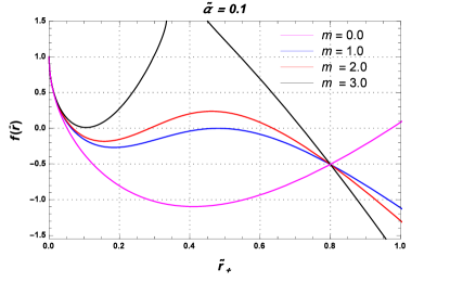
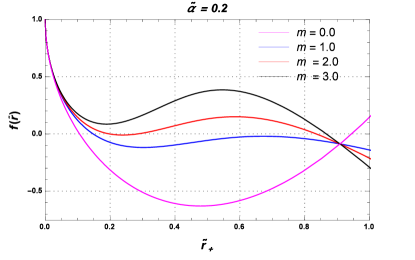
Figure 1: Metric function plot $f(r)$ as a function of horizon radius with the variation of massive gravity parameter $({m})$ for GB parameter ${\tilde{\alpha}}=0.1$ and ${\tilde{\alpha}}=0.2$. Here, $c=1,\tilde{c}_{1}=-1,c_{2}=1$.

	$\tilde{\alpha}=0.1$					$\tilde{\alpha}=0.2$
$m$	$r_{-}$	$r_{+}$	$\delta$	$m$	$r_{-}$	$r_{+}$	$\delta$
0	0.1344	1.934	1.799	$0$	0.0963	1.865	1.768
1.50	0.3685	1.715	1.346	$1.50$	0.3716	1.5	1.128
2.09	0.3539	1.429	0.5996	1.73	0.5023	1.328	0.8257
2.50	0.3539	1.429	0.5996	1.90	0.5023	1.328	0.8257

Table 1: Cauchy ($\tilde{r}_{-}$) and event ($\tilde{r}_{+}$) horizons, and $\delta=\tilde{r}_{+}-\tilde{r}_{-}$ for the $4D$ AdS EGB massive black hole for GB parameter ${\tilde{\alpha}}=0.1$ and ${\tilde{\alpha}}=0.2$. Here, $c=1,\tilde{c}_{1}=-1,c_{2}=1$.

From Fig. 1, it is clear that the size of the black hole increases with a decrease in the GB parameter. The black hole has three (Cauchy, event, and cosmological) horizons at $m>2.09$ with $\tilde{\alpha}=0.1$. However, the event and cosmological horizons are possible for $m<2.09$. The horizon is a decreasing function of massive parameter ($m$) (Fig. 1 right panel), an increasing function of massive gravity parameter and finally independent of GB parameter (Fig. 1 right panel). It should be pointed out that interestingly, increasing and decreasing mentioned parameters, will lead to formation of the different sized black hole.

III Thermodynamics

In this section, we study the thermodynamic properties of $4D$ $AdS$ Gauss-Bonnet massive black hole. In particular, these are mass $(\tilde{M}_{+})$, temperature $(\tilde{T}_{+})$, entropy $(\tilde{S}_{+})$ and free energy $(\tilde{G}_{+})$. The mass of the black hole is derived by setting $f_{-}(\tilde{r})|_{\tilde{r}=\tilde{r}_{+}}=0$ as

$$\tilde{M}_{+}=\frac{1}{2\tilde{r}_{+}}\left[\tilde{r}_{+}^{2}+\tilde{\alpha}+{\tilde{r}_{+}^{4}}+{m^{2}\tilde{r}_{+}^{2}}\left(\frac{c\tilde{c}_{1}\tilde{r}_{+}}{2}+2c^{2}c_{2}\right)\right].$$ (18)

The Hawking temperature for this black hole solution can be estimated from the well-known area-law

$$\tilde{T}_{+}=\frac{1}{4\pi}f^{\prime}(\tilde{r})|_{\tilde{r}=\tilde{r}_{+}},$$ (19)

as follows

$$\tilde{T}_{+}=T_{+}l=\frac{1}{4\pi\tilde{r}_{+}(r_{+}^{2}+2\tilde{\alpha})}\left[\tilde{r}_{+}^{2}-\tilde{\alpha}+{3\tilde{r}_{+}^{4}}+m^{2}\tilde{r}_{+}^{2}(c^{2}c_{2}+c\tilde{c}_{1}\tilde{r})\right].$$ (20)

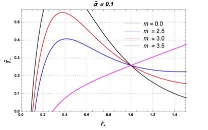
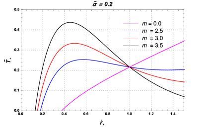
Figure 2: Temperature plot $(\tilde{T}_{+})$ as a function of horizon radius with the variation of massive gravity parameter $(m)$ for GB parameter $\tilde{\alpha}=0.1$ and $\tilde{\alpha}=0.2$. Here, $c=1,\tilde{c}_{1}=-1,c_{2}=1$.

It is evident Fig. 2 that the temperature is negative when the two (Cauchy and event) horizons merge, therefore, in this region, the obtained solutions are not physical.

The thermodynamical quantities must follow the first law of thermodynamics

$$d\tilde{M}_{+}=\tilde{T}d\tilde{S}_{+}.$$ (21)

This leads to explicit expression for entropy $\tilde{S}_{+}=\int\frac{d\tilde{M}_{+}}{\tilde{T}_{+}}d\tilde{r}_{+}$ as [28, 45]

$$\tilde{S}_{+}=\pi\tilde{r}_{+}^{2}+4\pi\tilde{\alpha}\log[\tilde{r}]+\tilde{S}_{0},$$ (22)

where $\tilde{S}_{0}$ is an integration constant.

It is worth mentioning that the definition of first-law of thermodynamics may have additional terms also in the extended phase space. In order to check the validity of these terms one should check the first-law in the non-differential form called as the Smarr relation

$$\tilde{M}_{+}=2\tilde{T}_{+}\tilde{S}_{+}+2\tilde{V}_{+}\tilde{P}-\tilde{A}\tilde{\alpha}-{\cal\tilde{C}}\tilde{c}_{1},$$ (23)

where

$$\tilde{P}=-\frac{\Lambda}{8\pi},\qquad\qquad\qquad\qquad\quad\tilde{V}_{+}=\left(\frac{\partial\tilde{M}_{+}}{\partial\tilde{P}}\right)_{\tilde{S}_{+},\tilde{\alpha},\tilde{c}_{1}},$$ (24)

$${\cal\tilde{C}}=\left(\frac{\partial\tilde{M}_{+}}{\partial\tilde{c}_{1}}\right)_{\tilde{S}_{+},\tilde{\alpha},\tilde{P}},\qquad\qquad\qquad\tilde{A}=\left(\frac{\partial\tilde{M}_{+}}{\partial\tilde{\alpha}}\right)_{\tilde{S}_{+},\tilde{P},\tilde{c}_{1}}.$$ (25)

From all the above additional thermodynamic quantities, it is easy to verify the complete form of the first-law of thermodynamics in an extended space

$$d\tilde{M}_{+}=\tilde{T}_{+}d\tilde{S}_{+}-\tilde{V}_{+}d\tilde{P}+\tilde{A}d\tilde{\alpha}+{\cal\tilde{C}}dc_{1}.$$ (26)

To understand the global stability of the black hole, the behavior of the Gibbs free energy $\tilde{G}_{+}$ is important to analyzed. The Gibbs free energy, from the definition $\tilde{G}_{+}=\tilde{M}_{+}-\tilde{T}_{+}\tilde{S}_{+}$, is derived by

$$\tilde{G}_{+} = \frac{1}{2\tilde{r}_{+}}\left[\tilde{r}_{+}^{2}+2\tilde{\alpha}+{\tilde{r}_{+}^{3}}+m^{2}\left(\frac{c\tilde{c}_{1}\tilde{r}_{+}^{2}}{2}+c^{2}c_{2}\tilde{r}_{+}\right)\right]$$ (27)

$$- \frac{(\tilde{r}_{+}^{2}+4\alpha\log[\frac{\tilde{r}}{\tilde{r}_{0}}])}{4\tilde{r}_{+}(\tilde{r}_{+}^{2}+2\tilde{\alpha})}\left[\tilde{r}_{+}^{2}-\tilde{\alpha}+{3\tilde{r}_{+}^{4}}+m^{2}\tilde{r}_{+}^{2}(c^{2}c_{2}+c\tilde{c}_{1}\tilde{r})\right].$$

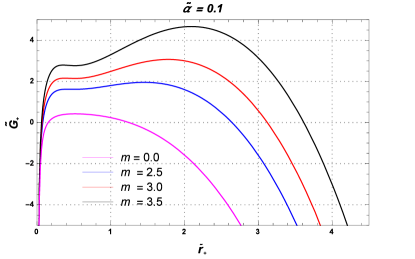
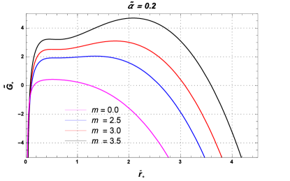
Figure 3: Plot of free energy $(\tilde{G}_{+})$ as a function of horizon radius with the variation of massive gravity parameter $(m)$ for GB parameter $\tilde{\alpha}=0.1$ and $\tilde{\alpha}=0.2$. Here, $c=1,c_{1}=-1,c_{2}=1$.

To analyze Gibbs free energy, we plot figure 3 for different values of massive gravity parameter and GB parameter. Here, we see that Gibbs free energy increases with GB parameter. However, with increasing $m$ the Gibbs free energy first increases and then starts falling after a critical point.

IV Heat Capacitity and thermodynamics stability

Now, we study the heat capacity of the obtained black hole solution (12) in the context of canonical ensemble by calculating the heat capacity. The heat capacity is given by the following relation:

$$\tilde{C}_{+}=\left(\frac{\partial\tilde{M}_{+}}{\partial\tilde{T}_{+}}\right)_{\tilde{\alpha}}=\left(\frac{\tilde{\partial}M_{+}}{\tilde{\partial}r_{+}}\right)_{\tilde{\alpha}}\left(\frac{\partial\tilde{r}_{+}}{\partial\tilde{T}_{+}}\right)_{\tilde{\alpha}}.$$ (28)

Substituting the value of mass from (18) and temperature from (20) in Eq. (28), we get

$$\tilde{C}_{+}=\frac{{2\pi\tilde{r}^{2}(\tilde{r}^{2}+2\tilde{\alpha})^{2}}\left(1+c^{2}c_{2}\tilde{m}^{2}+c\tilde{c}_{1}m^{2}r+{3\tilde{r}^{2}}-\frac{\tilde{\alpha}}{\tilde{r}^{2}}\right)}{3(\tilde{r}^{6}+6\tilde{r}^{4}\tilde{\alpha})+[-(1+c^{2}c_{2}m^{2})\tilde{r}^{4}+(5+2c^{2}c_{2}m^{2})\tilde{r}^{2}\tilde{\alpha}+4c\tilde{c}_{1}m^{2}\tilde{r}^{3}\tilde{\alpha}+2\tilde{\alpha}^{2}]}.$$ (29)

Figure 4: Plot of heat capacity ($\tilde{C}_{+}$) as a function of horizon radius with the variation of massive gravity parameter $(m)$ for GB parameter $\tilde{\alpha}=0.2$ with fixed value of $c=1,\tilde{c}_{1}=-1,c_{2}=1$.

In order to study the thermodynamical behavior of the system stability and phase transition points, we plot this thermodynamics quantity in Fig. 4. For Eq. (29), the heat capacity will have divergences at extremum points.

We know that roots and divergences present in the heat capacity represent phase transition points of the system. Additionally, we should mention that unstable systems undergo a phase transition and becomes stable. Corresponding to the root there exists a phase transition from unstable (non-physical) system to stable (physical) one. For small divergence a phase transition from large black holes to small ones takes place and for large divergence a phase transition occurs from smaller black holes to larger ones.

V Phase transition of 4D EGB Massive black hole

In the extended phase space, the mass of the black hole treated as the enthalpy rather then the internal energy of the system. The cosmological constant is treated as the thermodynamics pressure $(\Lambda=-8\pi P)$ [42, 43] and corresponding conjugate quantity is volume which is given by

$$\tilde{V}_{+}=\frac{4}{3}\pi\tilde{r}_{+}^{3}.$$ (30)

The equations of state (EOS) can obtained by relation (23) and Hawking temperature as

$$\tilde{P}_{+}=\frac{\tilde{T}_{+}}{2\tilde{r}_{+}}+\frac{\tilde{T}_{+}\alpha}{\tilde{r}_{+}^{3}}+\frac{\tilde{\alpha}}{8\pi\tilde{r}_{+}^{4}}-\frac{1}{8\pi\tilde{r}_{+}^{2}}-\frac{m^{2}}{8\pi\tilde{r}_{+}^{2}}\left(c\tilde{c}_{1}\tilde{r}+c^{2}c_{2}\right),\qquad\qquad\tilde{v}=2\tilde{r}_{+},$$ (31)

where $\tilde{v}$ represents specific volume. Using the properties of the inflection points we can encode the information about the EoS in the critical points. The critical point occurs when $\tilde{P}_{+}$ has an inflection point

$$\frac{\partial\tilde{P}_{+}}{\partial\tilde{v}}=\frac{\partial^{2}\tilde{P}_{+}}{\partial\tilde{v}^{2}}=0.$$ (32)

The corresponding critical point is determined by the following equation:

$$\tilde{r}_{+}^{4}-12\tilde{\alpha}(\tilde{r}_{+}^{2}+\tilde{\alpha})+m^{2}\tilde{r}_{+}^{2}(c^{2}c_{2}\tilde{r}_{+}^{2}-6\tilde{\alpha}(c^{2}c_{2}+c\tilde{c}_{1}\tilde{r}_{+}))=0.$$ (33)

$m$	$\tilde{r}_{C}$	$\tilde{T}_{C}$	$\tilde{P}_{C}$	$\frac{\tilde{P}_{C}\,\tilde{v}_{C}}{\tilde{T}_{C}}$
0	1.1370	0.0808	0.0126	0.3546
1	0.8525	0.1327	0.0440	0.5653
2	0.6714	0.3267	0.1666	0.6847
3	0.6050	0.6770	0.3920	0.7006
4	0.5757	1.1598	0.7164	0.7112
5	0.5606	1.7913	1.1373	0.7118
$\tilde{\alpha}$
0.1	0.8525	0.1327	0.0440	0.5653
0.2	1.1403	0.0214	0.0251	0.7028
0.3	1.3397	0.0590	0.0184	0.8356
0.4	1.4951	0.0459	0.0150	0.9771
0.5	1.6231	0.0370	0.0129	1.1317

Table 2: The table for critical temperature $\tilde{T}_{C}$, critical pressure $\tilde{P}_{C}$ and ${\tilde{P}_{C}\,\tilde{v}_{C}}/{\tilde{T}_{C}}$ corresponding different value of $m$ with fixed value of $c=1,\tilde{c}_{1}=-0.75,c_{2}=0.75$ and $\tilde{\alpha}=0.1$.

We find that Eq. (33) can not be solve analytically. In order to estimate the critical points, namely, critical horizon radius ($\tilde{r}_{C}$), critical temperature ($\tilde{T}_{+}$) and critical pressure $(\tilde{P}_{+})$ the numerical solutions of Eq. (33) with variation of massive parameter and and GB coupling are tabulated in the Table (II) and Table (III). It is interesting to see that the critical pressure and critical temperature increase with increasing critical radius and massive parameter at $\tilde{\alpha}=0.1$. However, the critical pressure and critical temperature decrease with increasing critical radius and GB coupling parameter for $m=1$.

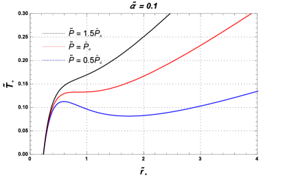
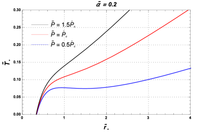
Figure 5: The plots of temperature vs horizon radius for $\tilde{\alpha}=0.1$ (left) and $\tilde{\alpha}=0.2$ (right) with fixed values of $c=1,\tilde{c}_{1}=-1,c_{2}=1$ and $m=1$ .

We study the phase transition by analyzing the Gibbs free energy for different values of massive gravity parameter $(m)$ and GB coupling $(\alpha)$ as depicted from Fig. 6. The characteristic swallow tail confirms that the obtained values are the critical ones in which the phase transition takes place. The thermodynamically stable (unstable) state occurs corresponding to the lowest (highest) Gibbs free energy. As a result, the triangular loop in the $\tilde{G}_{+}-\tilde{T}_{+}$ plane represents an unstable state. The straight line corresponds to the first order phase transition as the temperature rises in the system, as shown in the $\tilde{T}_{+}-\tilde{r}_{+}$ plane (Fig. 7). The curved portion of the isobar indicates the unstable state due to the system’s possessing lower Gibbs free energy. We note that the net change in Gibbs free energy around the triangular loop is zero.

We can also see that swallow tail shape occurs in case of $\tilde{P}_{+}<\tilde{P}_{c}$ for the first order phase transition. However, in case of $\tilde{P}_{+}=\tilde{P}_{c}$, the second order phase transition occurs. The intercepts of the axis in the $\tilde{G}_{+}-\tilde{T}_{+}$ plane decrease as the GB coupling parameter and mass gravity parameter increase, whereas the intercepts of the $\tilde{G}$ -axis increase as the GB coupling parameter and mass gravity parameter increase.

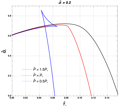
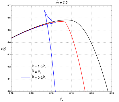
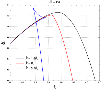
Figure 6: The plots of Gibbs free energy ($\tilde{G}_{+}$) vs temperature ($\tilde{T}_{+}$) for $\alpha=0.1$ (upper left), $\alpha=0.2$ (upper right), $m=1.0$ (lower left) and $m=2.0$ (lower right) with fixed values of $c=1,\tilde{c}_{1}=-0.7,c_{2}=0.75$ .

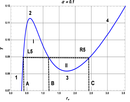
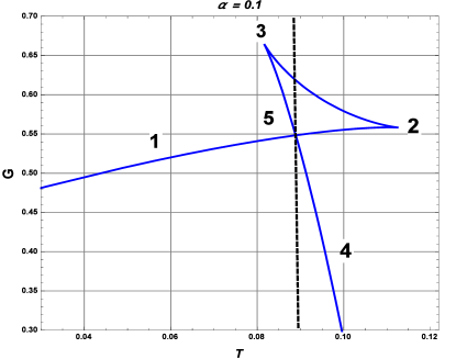
Figure 7: The plots of temperature ($\tilde{T}_{+}$) vs horizon radius $(\tilde{r}_{+})$ and Gibbs free energy ($\tilde{G}_{+}$) vs temperature ($\tilde{T}_{+}$) with fixed values of $\tilde{\alpha}=0.1$ and for $m=1.0$ and $m=2.0$ $c=1,\tilde{c}_{1}=-1,c_{2}=1$.

When the temperature is lower than the critical temperature in the $\tilde{T}_{+}-\tilde{r}_{+}$ plot, we can see three black holes (small, intermediate, and large) for the $4DAdS$ EGB massive black hole with the same massive gravity parameter of $m$ for a specific temperature range. The small and large black holes are stable, but the intermediate black hole is unstable, since the heat capacity $\tilde{C}_{+}$ is negative (see Fig. 4). Because of the small free energy, $\tilde{T}_{+}<T_{\star}$ corresponds to a small black hole, and $\tilde{T}_{+}>T_{\star}$ corresponds to a large black hole, where $T_{\star}$ is the transition temperature, which has values of $0.088$ and $0.048$ for $\tilde{\alpha}=0.1$ and $\tilde{\alpha}=0.2$, respectively. Due to the same free energy, black holes can transit from one phase to another phase at a critical temperature. In Fig. 7, point 5 represents the coexistence of small and large black holes. The small black holes are represented by the solid lines $1-L5$ or $1-5$, while the large black holes are represented by the solid lines $R5-4$ or $5-4$. We noticed that the point $L5$ and $R5$ share the same free energy.

VI Curvature Singularity and Phase Transition new thermodynamic geometry

we have proposed a new formalism of the thermodynamic geometry (NTG) which explains the one-to-one correspondence between phase transitions and singularities of the scalar curvature [44, 45].The NTG geometry is defined as

$$dl^{2}_{NTG}=\frac{1}{T}\left(n^{j}_{i}\frac{\partial^{2}\Xi}{\partial X^{i}\partial X^{j}}dX^{i}dX^{j}\right),$$ (34)

where $(n^{j}_{i}=\text{diag}(-1,1,1,\ldots 1)$ and $Xi$ is thermodynamic potential [44] and the geometrothermodynamics (GTD) metric is conformally related to NTG metric such that this conformal transformation is singular at unphysical points were generated in GTD metric [44].

To study the curvature singularity and phase transition in NTG. We write the free energy in term of specific volume and temperature

$$\tilde{G}_{+} = \frac{1}{\tilde{v}_{+}}\left[\frac{\tilde{v}_{+}^{2}}{4}+2\tilde{\alpha}+\frac{\tilde{v}_{+}^{3}}{8}+m^{2}\left(\frac{c\tilde{c}_{1}\tilde{v}_{+}^{2}}{8}+\frac{c^{2}c_{2}\tilde{v}_{+}}{2}\right)-(\frac{\tilde{v}_{+}^{2}}{4}+4\alpha\log[\frac{\tilde{r}}{2}])\tilde{T}\right].$$ (35)

The differential form of free energy $d\tilde{F}_{+}=-\tilde{S}_{+}d\tilde{T}_{+}-\tilde{P}d\tilde{V}_{+}+\tilde{A}d\tilde{\alpha}+\tilde{\cal C}d\tilde{c}_{1}$ combining with Eq. (35), we deduce

$$\tilde{S}_{+}=-\left(\frac{\partial\tilde{F}_{+}}{\partial\tilde{T}_{+}}\right)_{\tilde{V},\tilde{\alpha},{\cal\tilde{C}}}=\frac{\pi}{4}\left[\tilde{v}^{2}+16\tilde{\alpha}\log\left(\frac{\tilde{v}}{\tilde{v}_{0}}\right)\right],$$ (36)

$$\tilde{P}=-\left(\frac{\partial\tilde{F}_{+}}{\partial\tilde{V}_{+}}\right)_{\tilde{V},\tilde{\alpha},{\cal\tilde{C}}}=\frac{\tilde{T}_{+}}{\tilde{v}_{+}}+\frac{8\tilde{v}_{+}\alpha}{\tilde{r}_{+}^{3}}+\frac{2\tilde{\alpha}}{\pi\tilde{v}_{+}^{4}}-\frac{1}{2\pi\tilde{v}_{+}^{2}}-\frac{m^{2}}{2\pi\tilde{v}_{+}^{2}}\left(\frac{c\tilde{c}_{1}\tilde{v}_{+}}{2}+c^{2}c_{2}\right),$$ (37)

$$\tilde{A}=-\left(\frac{\partial\tilde{F}_{+}}{\partial\tilde{\alpha}}\right)_{\tilde{V},\tilde{\alpha},{\cal\tilde{C}}}=\frac{1}{\tilde{v}}-4\pi\tilde{T}_{+}\log\left(\frac{\tilde{v}}{\tilde{v}_{0}}\right),$$ (38)

$${\cal\tilde{C}}=-\left(\frac{\partial\tilde{F}}{\partial\tilde{c}_{1}}\right)_{\tilde{V},\tilde{\alpha},{\cal\tilde{C}}}=\frac{m^{2}\tilde{c}_{1}\tilde{v}^{2}}{16}.$$ (39)

The phase transition is appear when a heat capacity diverges, when $\tilde{C}_{+}>0$ the system is stable and $\tilde{C}_{+}<0$ the system is unstable. The heat capacity is written as

$$\tilde{C}_{+}=\frac{{2\pi\tilde{r}^{2}(\tilde{r}^{2}+2\tilde{\alpha})^{2}}\left(1+c^{2}c_{2}m^{2}+c\tilde{c}_{1}m^{2}r+{3\tilde{r}^{2}}-\frac{\tilde{\alpha}}{\tilde{r}^{2}}\right)}{3(\tilde{r}^{6}+6\tilde{r}^{4}\tilde{\alpha})+[-(1+c^{2}c_{2}m^{2})\tilde{r}^{4}+(5+2c^{2}c_{2}m^{2})\tilde{r}^{2}\tilde{\alpha}+4c\tilde{c}_{1}m^{2}\tilde{r}^{3}\tilde{\alpha}+2\tilde{\alpha}^{2}]}.$$ (40)

Now, we are able to implement the NTG geometry to analysis the phase transition behaviour of heat capacity (40). By substituting the $\Xi=\tilde{H}=\tilde{M}_{+}+\tilde{E}+\tilde{P}\tilde{V}_{+}$ with $X^{i}=(\tilde{S}_{+},\tilde{P},\tilde{\alpha},{\cal\tilde{C}})$ into Eq. (34), we have

$$g_{H}^{NTG}=\begin{bmatrix}-\left(\frac{\partial\tilde{T}_{+}}{\partial\tilde{S}_{+}}\right)_{\tilde{P},\tilde{c}_{1},\tilde{\alpha}}&0&0&0\\ 0&\left(\frac{\partial\tilde{V}_{+}}{\partial\tilde{S}_{+}}\right)_{\tilde{S}_{+},\tilde{c}_{1},\tilde{\alpha}}&\left(\frac{\partial\tilde{V}_{+}}{\partial\tilde{c}_{1}}\right)_{\tilde{S}_{+},\tilde{P},\tilde{\alpha}}&\left(\frac{\partial\tilde{A}}{\partial\tilde{P}}\right)_{\tilde{S}_{+},\tilde{c}_{1},\alpha}\\ 0&\left(\frac{\partial\tilde{V}_{+}}{\partial\tilde{C}}\right)_{\tilde{S}_{+},\tilde{P},\tilde{\alpha}}&\left(\frac{\partial\tilde{C}}{\partial\tilde{c}_{1}}\right)_{\tilde{S}_{+},\tilde{P},\tilde{\alpha}}&\left(\frac{\partial\tilde{A}}{\partial\tilde{c}_{1}}\right)_{\tilde{S}_{+},\tilde{P},\tilde{\alpha}}\\ 0&\left(\frac{\partial\tilde{A}}{\partial\tilde{P}}\right)_{\tilde{S}_{+},\tilde{c}_{1},\tilde{\alpha}}&\left(\frac{\partial\tilde{A}}{\partial\tilde{c}_{1}}\right)_{\tilde{S}_{+},\tilde{P},\tilde{\alpha}}&\left(\frac{\partial\tilde{A}}{\partial\tilde{\alpha}}\right)_{\tilde{S}_{+},\tilde{c}_{1},\tilde{P}}\end{bmatrix}$$

.

Since all thermodynamic parameters are written as a function of $(\tilde{T}_{+},\tilde{v},\tilde{c}_{1},\tilde{\alpha})$, it is convenient to recast metric elements from the coordinate $X_{i}=(\tilde{S},\tilde{P},\tilde{c}_{1},\tilde{\alpha})$ to the coordinate $(\tilde{T}_{+},\tilde{v},\tilde{c}_{1},\tilde{\alpha})$ by using the following Jacobians

$$J=\frac{\partial(\tilde{S}_{+},\tilde{P},{\cal\tilde{C}},\tilde{\alpha})}{(\tilde{T}_{+},\tilde{v},{\cal\tilde{C}},\tilde{\alpha})}=\begin{bmatrix}0&\pi\left(\frac{\tilde{v}}{2}+\frac{4\tilde{\alpha}}{\tilde{v}}\right)&0&{4\pi\log\left(\frac{\tilde{v}}{\tilde{v}_{0}}\right)}\\ \frac{\tilde{v}^{2}+8\tilde{\alpha}}{\tilde{v}^{3}}&\frac{\tilde{v}^{2}-\pi\tilde{T}_{+}\tilde{v}^{3}-8\tilde{(}1+3\pi\tilde{T}\tilde{v})}{\pi\tilde{v}^{5}}+\frac{m^{2}(4c^{2}c_{2}+c\tilde{c}_{1}\tilde{v}))}{4\pi\tilde{v}^{3}}&-\frac{m^{2}}{2\pi\tilde{v}_{+}^{2}}\left(\frac{\tilde{c}_{1}\tilde{v}}{2}+2cc_{2}\right)&\frac{2(1+4\pi\tilde{T}\tilde{v})}{\pi\tilde{v}^{4}}\\ 0&0&1&0\\ 0&0&0&1\end{bmatrix}$$

Finally the metric element convert to

$${\hat{g}}=J^{T}g_{H}^{NTG}J=\begin{bmatrix}0&0&0&-\frac{4\pi}{\tilde{T}_{+}}\log\left(\frac{\tilde{v}}{\tilde{v}_{0}}\right)\\ 0&\frac{\tilde{v}^{2}-\pi\tilde{T}_{+}\tilde{v}^{3}-8\tilde{(}1+3\pi\tilde{T}_{+}\tilde{v})}{\pi\tilde{T}_{+}\tilde{v}^{3}}+\frac{m^{2}(4c^{2}c_{2}+c\tilde{c}_{1}\tilde{v}))}{4\pi\tilde{T}_{+}\tilde{v}}&0&0\\ 0&0&\frac{2}{\tilde{T}_{+}\tilde{v}}&0\\ -\frac{4\pi}{\tilde{T}_{+}}\log\left(\frac{\tilde{v}}{\tilde{v}_{0}}\right)&0&0&0\end{bmatrix}$$

. The denominator of the scalar curvature is

$$D(R^{NTG})=\pi\left(\frac{\tilde{v}^{2}-\pi\tilde{T}_{+}\tilde{v}^{3}-8(1+3\pi\tilde{T}_{+}\tilde{v})}{\pi\tilde{v}^{5}}+\frac{m^{2}(4c^{2}c_{2}+c\tilde{c}_{1}\tilde{v}))}{4\pi\tilde{v}^{3}}\right)^{2}\log\left(\frac{\tilde{v}}{\tilde{v}_{0}}\right)$$ (41)

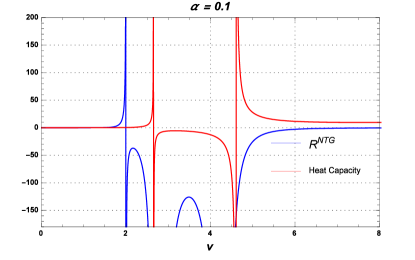
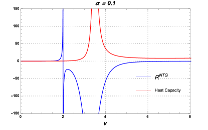
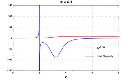
Figure 8: The plots of heat capacity and scalar curvature vs specific volume for $\tilde{\alpha}=0.1$, $m=2.0$ with fixed values of $c=1,\tilde{c}_{1}=-1.0,c_{2}=1.0$ for $\tilde{T}_{+}<\tilde{T}_{c},\tilde{T}_{+}=\tilde{T}_{c}$ and $\tilde{T}_{+}>\tilde{T}_{c}$, where $\tilde{T}_{c}=0.3267$.

The plot of scalar curvature and heat capacity with respect to specific volume are depicted Fig. 8. We observe that from the Fig. 8, there is two divergence for heat capacity at $\tilde{T}_{+}<\tilde{T}_{c}$ and there are three possible phases i.e., the small black hole (SBH), intermediate black hole (IBH) and large black hole (LBH). At $\tilde{T}_{+}=\tilde{T}_{c}$, these divergent points get closer and coincide to form a single divergent point. We noticed that at $\tilde{T}_{+}>\tilde{T}_{c}$ the heat capacity is positive and there is no phase transition, it means that the black hole is stable. The scalar curvature is positive in the range of $0<\tilde{v}<\tilde{v}_{0}=1.7$ that implies a repulsive interaction between the microscopic black hole molecules.

VII Conclusions

We have found a singular solution to the massive EGB gravity in $4D$ $AdS$ spacetime. In fact, we obtain both positive and negative branches of solutions in which one is not physically correct and therefore can be dropped. The horizon structure of the black hole is also discussed. We have found that the real roots of the physically correct metric lead to three horizons (Cauchy, event, and cosmological horizons) below a certain graviton mass limit. However, only two horizons (event and cosmological horizons) are possible after this mass limit.

The thermal properties of this black hole solution are also discussed in a standard way. We derived the mass of the black hole by setting the metric function to zero. The Hawking temperature is calculated from the well-known area-law. We have seen that the black hole solution is not physical when Cauchy and event horizons merge. We have further checked the validity of the first law of black hole chemistry. Gibbs energy is also derived. In order to check the stability of the black hole, we have computed its heat capacity. Here we have one root and two divergent points. Finally, we have described the effects of massive graviton and GB parameters on the phase transition and critical points of the system. We have observed that the critical pressure and critical temperature increase with increasing critical radius and graviton mass. In contrast, the critical pressure and critical temperature decrease as the critical radius and GB parameter increase. In fact, black holes undergo a phase transition at a critical temperature. In the Gibbs free energy plots we have seen characteristic swallow tail which locates the critical point where phase transition takes place.

References

- [1] C. Barrabes and G.F. Bressange, Class. Quant. Grav. 14 (1997) 805.
- [2] R.-G. Cai and Y.S. Myung, Phys. Rev. D 56 (1997) 3466.
- [3] S. Capozziello and A. Troisi, Phys. Rev. D 72 (2005) 044022.
- [4] T.P. Sotiriou, Class. Quant. Grav. 23 (2006) 5117.
- [5] J.W. Moffat, JCAP 03 (2006) 004.
- [6] V. Faraoni, Phys. Rev. D 75 (2007) 067302.
- [7] K.-i. Maeda and Y. Fujii, Phys. Rev. D 79 (2009) 084026.
- [8] D. Lovelock, J. Math. Phys. 12 (1971) 498.
- [9] D. Lovelock, J. Math. Phys. 13 (1972) 874.
- [10] N. Deruelle and L. Farina-Busto, Phys. Rev. D 41 (1990) 3696.
- [11] J.M. Cline and H. Firouzjahi, Phys. Rev. D 64 (2001) 023505.
- [12] T. Nihei, N. Okada and O. Seto, Phys. Rev. D 71 (2005) 063535.
- [13] M. Demetrian, Gen. Rel. Grav. 38 (2006) 953.
- [14] C. Lanczos, Ann. Math. 39, 842 (1938).
- [15] R. Cai, Phys. Rev. D 65, 084014 (2002).
- [16] H. C.D. Lima Junior, C. L.Benone and L. C.B. Crispino, Phys. Lett. B 811 (2020) 135921.
- [17] M. Fierz, Helv. Phys. Acta 12 (1939) 3.
- [18] D. G. Boulware and S. Deser, Phys. Rev. D 6 (1972) 3368.
- [19] S. H. Hendi, S. Panahiyan, S. Upadhyay and B. Eslam Panah, Phys. Rev. D 95, 084036 (2017).
- [20] S. Upadhyay, S. H. Hendi, S. Panahiyan and B. Eslam Panah, Prog. Theor. Exp. Phys. 093E01, 1-20 (2018).
- [21] S. H. Hendi, S. Panahiyan and B. Eslam Panah, JHEP 01, 129 (2016).
- [22] D. Glavan and C. Lin, Phys. Rev. Lett. 124, 081301 (2020).
- [23] K. Aolki, M. A. Gorji and S. Mukohyama, Phys. Lett. B 810 (2020) 135843.
- [24] K. Aolki, M. A. Gorji and S. Mukohyama, JCAP 2009 (2020) 014.
- [25] P. G. S. Fernandes, Phys. Lett. B 805 (2020), 135468.
- [26] R. A. Hennigar, D. Kubizňák, R. B. Mann and C. Pollack, JHEP 07 (2020) 027.
- [27] S. G. Ghosh, D. V. Singh, R. Kumar and S. D. Maharaj, Annals Phys. 424 (2021), 168347.
- [28] S. W. Wei and Y. X. Liu, Phys. Rev. D 101 (2020) no.10, 104018.
- [29] D. V. Singh, S. G. Ghosh and S. D. Maharaj, Phys. Dark Univ. 30 (2020) 100730.
- [30] D. V. Singh and S. Siwach, Phys. Lett. B. 408 135658 (2020).
- [31] D. V. Singh, B. K. Singh and S. Upadhyay, Annals Phys. 434 (2021), 168642.
- [32] B. K. Singh, R. P. Singh and D. V. Singh, Eur. Phys. J. Plus 136 (2021) no.5, 575.
- [33] B. K. Singh, R. P. Singh and D. V. Singh, Eur. Phys. J. Plus 135 (2020) no.10, 862.
- [34] N. Godani, D. V. Singh and G. C. Samanta, Phys. Dark Univ. 35 (2022), 100952.
- [35] S. H. Hendi, M. Momennia, J. High Energ. Phys. 10 (2019) 207.
- [36] B. Eslam Panah, Kh. Jafarzade, S. H. Hendi, Nuclear Physics B 961 (2020) 115269.
- [37] S. H. Hendi, M. Momennia, Physics Letters B 777 (2018) 222.
- [38] S. H. Hendi, B. Eslam Panah, S. Panahiyan, M. S. Talezadeh, Eur. Phys. J. C 77 (2017) 133.
- [39] S. H. Hendi, B. Eslam Panah, S. Panahiyan ,Class. Quant. Grav. 33 (2016) 235007.
- [40] S. H. Hendi, S. Panahiyan, Phys. Rev. D 90 (2014) 124008.
- [41] S. H. Hendi, B. E. Panah and S. Panahiyan, Fortsch. Phys. 66 (2018) no.3, 180000.
- [42] D. Kubiznak and R.B. Mann, JHEP 07 (2012) 033.
- [43] S. Gunasekaran, R.B. Mann and D. Kubiznak, JHEP 11 (2012) 110.
- [44] S. A. Hosseini Mansoori and B. Mirza, Phys. Lett. B 799 (2019), 135040
- [45] S. A. Hosseini Mansoori, Phys. Dark Univ. 31 (2021), 100776