New anisotropic star solutions in mimetic gravity

Abstract

We extract new classes of anisotropic solutions in the framework of mimetic gravity, by applying the Tolman-Finch-Skea metric and a specific anisotropy not directly depending on it, and by matching smoothly the interior anisotropic solution to the Schwarzschild exterior one. Then, in order to provide a transparent picture we use the data from the 4U 1608-52 pulsar. We study the profile of the energy density, as well as the radial and tangential pressures, and we show that they are all positive and decrease towards the center of the star. Furthermore, we investigate the anisotropy parameter and the anisotropic force, that are both increasing functions of the radius, which implies that the latter is repulsive. Additionally, by examining the radial and tangential equation-of-state parameters, we show that they are monotonically increasing, not corresponding to exotic matter. Concerning the metric potentials we find that they have no singularity, either at the center of the star or at the boundary. Furthermore, we verify that all energy conditions are satisfied, we show that the radial and tangential sound speed squares are positive and sub-luminal, and we find that the surface red-shift satisfies the theoretical requirement. Finally, in order to investigate the stability we apply the Tolman-Oppenheimer-Volkoff equation, we perform the adiabatic index analysis, and we examine the static case, showing that in all cases the star is stable.

I Introduction

Astrophysical compact objects, such as neutron stars and black holes, can serve as a crucial laboratory to investigate gravitational fields in the strong-field regime, and thus test General Relativity and its possible extensions Damour:1996ke ; Will:2014kxa ; Berti:2015itd ; LIGOScientific:2016lio ; Berti:2018cxi . Such extensions usually arise through the consideration of higher-order terms in the Einstein-Hilbert Lagrangian, such as in $fR)$ gravity DeFelice:2010aj , in Gauss-Bonnet and $f(G)$ gravity Antoniadis:1993jc ; Nojiri:2005jg , in Weyl gravity Mannheim:1988dj , in Lovelock and f$($Lovelock$)$ gravity Lovelock:1971yv ; Deruelle:1989fj , in scalar-tensor theories Fierz:1956zz ; Jordan:1959eg ; Brans:1961sx ; Damour:1992we etc (for a review see CANTATA:2021ktz ). Additionally, one may construct different classes of modifications by modifying the equivalent, torsional formulation of gravity, resulting in $f(T)$ gravity Bengochea:2008gz ; Cai:2015emx , in $f(T,T_{G})$ gravity Kofinas:2014owa , in scalar-torsion theories Geng:2011aj etc. Hence, in the literature one may find many studies of spherically symmetric solutions in the framework of modified gravity Garfinkle:1990qj ; Kanti:1995vq ; Cai:2001dz ; Kanti:2004nr ; Emparan:2008eg ; Nojiri:2010wj ; Kiritsis:2009rx ; Gonzalez:2011dr ; Pani:2011mg ; Pani:2011xm ; Capozziello:2012zj ; Nojiri:2017ncd ; Anabalon:2013oea ; Garattini:2014rwa ; Cai:2012db ; Nashed:2013bfa ; Astashenok:2015qzw ; Cisterna:2014nua ; Paliathanasis:2014iva ; Lu:2015cqa ; Moraes:2015uxq ; Astashenok:2015haa ; Babichev:2015rva ; Erices:2017izj ; Doneva:2017jop ; Doneva:2017bvd ; Jasim:2018cos ; Roupas:2020nua ; Karakasis:2021rpn ; Nashed:2018efg ; Ren:2021uqb ; Mota:2022zbq ; Nashed:2018cth ; Kiorpelidi:2022kuo ; Chatzifotis:2022mob ; Zhao:2022gxl .

One class of gravitational modification with interesting applications is mimetic gravity Chamseddine:2013kea ; Chamseddine:2014vna , which can be obtained from general relativity through the isolation of the conformal degree of freedom in a covariant way, by applying the a re-parametrization of the physical metric in terms of a mimetic field and an auxiliary metric. In this way, the field equations exhibit an additional term arising from the mimetic field. Since in a cosmological framework this term may be considered to correspond to a dust fluid component, the theory could be applied to describe cold dark matter in a “mimetic” way. Nevertheless, mimetic gravity can be extended in many ways, interpreted as a modification of gravity Chamseddine:2014vna ; Nojiri:2014zqa ; Leon:2014yua ; Nashed:2016tbj ; Momeni:2015gka ; Matsumoto:2015wja ; Chamseddine:2016uef ; Dutta:2017fjw ; Nashed:2011fg ; Chamseddine:2016ktu ; Vagnozzi:2017ilo ; Casalino:2018tcd ; Nashed:2021sji ; Casalino:2018wnc ; Abbassi:2018ywq ; Zhong:2018tqn ; Nashed:2020kjh ; Odintsov:2015wwp ; Nojiri:2016vhu ; Sadeghnezhad:2017hmr ; Gorji:2019ttx ; Gorji:2018okn ; ElHanafy:2017sih ; Bouhmadi-Lopez:2017lbx ; Gorji:2017cai ; Firouzjahi:2018xob ; Chamseddine:2019bcn ; Nashed:2021pkc (for a review see (Sebastiani:2016ras, )). Since mimetic modified gravity have many interesting applications at the cosmological framework (among them the ability to alleviate the cosmological tensions Abdalla:2022yfr , and to track possible quantum-related defects Addazi:2021xuf ), an amount of research has been devoted to the investigation of the spherically symmetric solutions too Deruelle:2014zza ; Myrzakulov:2015sea ; Myrzakulov:2015kda ; Odintsov:2015cwa ; Nojiri:2017ygt ; Odintsov:2018ggm ; Oikonomou:2015lgy ; Gorji:2020ten ; Nashed:2018qag ; Chen:2017ify ; Nashed:2018aai ; Nashed:2018urj ; BenAchour:2017ivq ; Zheng:2017qfs ; Shen:2019nyp ; Sheykhi:2020fqf ; Nashed:2021ctg .

Mimetic theory does not exhibit any difference from general relativity in flat spacetime. Therefore, we will test the mimetic theory in the frame of stellar structure models using two equations of states and radial metric potential $g_{rr}$ and confront the output results with GR. Additionally, we are interested in extracting new anisotropic star solutions in mimetic gravity by imposing the Tolman-Finch-Skea metric Finch_1989 , and in particular to examine the stability of the solutions as well as the behavior of the anisotropy. The plan of the work is as follows. In Section II we briefly review mimetic gravity, presenting the field equations. In Section III we extract new classes of anisotropic solutions. Then in Section IV we use the data from the 4U 1608-52 pulsar in order to investigate numerically the features of the obtained anisotropic stars, namely the profile of the energy density, as well as the radial and tangential pressures, the anisotropy factor, and the radial and tangential equation-of-state parameters. In Section V we study the stability of the solutions, applying the Tolman-Oppenheimer-Volkoff (TOV) equation, the adiabatic index, and we examine the static case. Finally, in Section VI we summarize the obtained results.

II Mimetic gravity

In this section we briefly present mimetic gravity. Starting from general relativity and parametrizing the physical metric $g_{\mu\nu}$ introducing an auxiliary metric $\bar{g}_{\mu\nu}$ and a mimetic field $\phi$, we acquire Chamseddine:2013kea

$$g_{\mu\nu}=\bar{g}_{\mu\nu}\bar{g}^{\alpha\beta}\partial_{\alpha}\phi\partial_{\beta}\phi\,,$$ (1)

which implies that the physical metric remains invariant under conformal transformations of the auxiliary metric. Hence, one can easily extract the expression

$$g^{\mu\nu}\partial_{\mu}\phi\partial_{\nu}\phi={-}1\,,$$ (2)

which can then be applied as a Lagrange multiplier in an extended action, namely (Chamseddine:2014vna, )

$$S=\int d^{4}x\sqrt{-g}\left[\frac{R}{2\kappa^{2}}+\lambda\left(\partial^{\mu}\phi\partial_{\mu}\phi{+}1\right)+\mathcal{L}_{m}\right]\,,$$ (3)

with $\kappa^{2}$ is the gravitational constant, $R$ the Ricci scalar, and $\mathcal{L}_{m}$ the usual matter Lagrangian, in units where $c=1$.

One can extract the field equations by varying the action in terms of the physical metric, incorporating additionally its dependence on the mimetic field as well as the auxiliary metric, resulting to

$$\frac{1}{\kappa^{2}}G_{\mu\nu}=\lambda\partial_{\mu}\phi\partial_{\nu}\phi+T_{\mu\nu},$$ (4)

with $G_{\mu\nu}$ the Einstein tensor and $T_{\mu\nu}$ the standard matter energy-momentum tensor. Moreover, variation with respect to the Lagrange multiplier leads to the condition (2). Taking the trace of equation (4) we find the Lagrange multiplier to be $\lambda=G/\kappa^{2}-T$, where $G$ and $T$ are the traces of the Einstein tensor and the matter energy-momentum tensor respectively. Varying (3) with respect to the mimetic scalar field leads to

$$\nabla^{\mu}\left(\lambda\partial_{\mu}\phi\right)=0.$$ (5)

Lastly, the above equations can be elaborated in a more compact form, namely

$$G_{\mu}{}^{\nu}-(G-T)\partial_{\mu}\phi\partial^{\nu}\phi=\kappa^{2}T_{\mu}{}^{\nu}\,,$$ (6)

$$\nabla_{\mu}\left[(G-T)\partial^{\mu}\phi\right]=0\,.$$ (7)

In this work we consider $T_{\mu}{}^{\nu}$ to correspond to an anisotropic fluid, namely we impose the form

$$T_{\mu}{}^{\nu}{}=(p_{t}+\rho)u_{\mu}u^{\nu}-p_{t}\delta_{\mu}{}^{\nu}+(p_{r}-p_{t})\xi_{\mu}\xi^{\nu}\,,$$ (8)

where $u_{\mu}$ is the time-like vector defined as $u^{\mu}=[1,0,0,0]$ and $\xi_{\mu}$ is the space-like unit radial vector defined as $\xi^{\mu}=[0,1,0,0]$, such that $u^{\mu}u_{\mu}=-1$ and $\xi^{\mu}\xi_{\mu}=1$.

III Novel classes of anisotropic solutions

We are interested in extracting new classes of spherically symmetric solutions of the field equations (6),(7). For this purpose, we introduce the metric

$$ds^{2}=\left[h(r)h_{1}(r)\right]dt^{2}-h_{1}(r)dr^{2}-r^{2}\left(d\theta^{2}+r^{2}\sin^{2}\theta d\phi^{2}\right)\,,$$ (9)

where $h(r)$ and $h_{1}(r)$ are the two metric functions. Under this metric, the field equations (6),(7) give rise to the following non-linear differential equations:

$$\!\!\!\!\!\!\!\!\!\!\!\!\!\!\!\!\!\!\!\!{\frac{h^{\prime}_{1}r+h_{1}{}^{2}-h_{1}}{r^{2}\,h_{1}{}^{2}}}=\kappa^{2}\rho\,,$$ (10)

$$\!\!\!\!\!\!\!\!\!\!\!\!\!\!\!\!\!\!\!\!\frac{1}{2h_{1}{}^{4}{r}^{2}h^{2}}\Bigg{\{}2\,h_{1}{}^{4}h^{2}-2\,h^{\prime}_{1}rh^{2}h_{1}{}^{2}-2\,h^{\prime}rhh_{1}{}^{3}-2\,h^{2}h_{1}{}^{3}-2\,\phi^{\prime 2}{r}^{2}h^{2}h_{1}{}^{3}(\rho-p_{r}-2p_{t})$$

$$\ \ \ \ \,+4\,\phi^{\prime 2}(h^{2}h_{1}{}^{3}-h_{1}{}^{2}h^{2}-rh^{\prime}hh_{1}{}^{2})-2\,\phi^{\prime 2}{r}^{2}h^{\prime\prime}hh_{1}{}^{2}+2\,\phi^{\prime 2}{r}^{2}h^{\prime}_{1}{}^{2}h^{2}$$

$$\ \ \ \ \,-\phi^{\prime 2}{r}^{2}h^{\prime}h^{\prime}_{1}{}hh^{\prime}_{1}{}-2\,\phi^{\prime 2}{r}^{2}h^{\prime\prime}_{1}{}h^{2}h_{1}{}+\phi^{\prime 2}{r}^{2}h^{\prime 2}h_{1}{}^{2}\Bigg{\}}=-\kappa^{2}\,p_{r}\,,$$ (11)

$$\!\!\!\!\!\!\!\!\!\!\!\!\!\!\!\!\!\!\!\!\frac{2\,rh^{\prime}_{1}{}^{2}h^{2}-2\,h^{\prime}hh_{1}{}^{2}-2\,rh^{\prime\prime}hh_{1}{}^{2}-rh^{\prime}h^{\prime}_{1}{}hh_{1}{}-2\,r\,h^{\prime\prime}_{1}{}h^{2}h_{1}{}+rh^{\prime 2}h_{1}{}^{2}}{4rh^{2}h_{1}{}^{3}}=-\kappa^{2}\,p_{t}\,,$$ (12)

where $\phi\equiv\phi(r)$ and with primes denoting derivatives with respect to $r$. The system (10)-(12) consists of three independent equations for six unknown functions; $h$, $h_{1}$, $\rho$, $p_{r}$, $p_{t}$, and $\phi$. Hence, we require to impose three extra conditions. We will try to solve the above system assuming the two equations of state:

$$p_{r}=\omega_{1}\rho\,,$$

and

$$p_{T}=\omega_{2}\rho\,,$$

and by imposing the condition $\phi=\int\sqrt{-g_{rr}}dr=\int\sqrt{h_{1}}dr$ we get the following system:

$$-{\frac{-hh^{\prime}_{1}r-h^{\prime}rh_{1}+hh_{1}{}^{2}-hh_{1}}{h_{1}{}^{2}h{r}^{2}}}=-{\frac{\omega_{1}\,\left(h^{\prime}_{1}r+h_{1}{}^{2}-h_{1}\right)}{h_{1}^{2}{r}^{2}}}\,,$$

$$\frac{-2\,rh^{\prime\prime}_{1}h^{2}h_{1}-2\,rh^{\prime\prime}hh_{1}{}^{2}+rh^{\prime 2}h_{1}{}^{2}-hh_{1}\left(2\,h_{1}+h^{\prime}_{1}r\right)h^{\prime}+2\,rh^{\prime}_{1}{}^{2}h^{2}}{4rh^{2}h_{1}{{}^{3}}}=-{\frac{\omega_{2}\,\left(h^{\prime}_{1}r+h_{1}{}^{2}-h_{1}\right)}{h_{1}{}^{2}{r}^{2}}}\,,$$

where $\omega_{1}$ and $\omega_{2}$ are the parameters characterizing the fluid. The above differential equations, (III) have no analytical solution except for the case of dust, i.e., $\omega_{1}=\omega_{2}=0$, the vacuum case otherwise, we cannot find any analytical solution that can extract from it any physics.

Other way to solve equations (10)-(12) is to assume the expression of the metric potential $g_{rr}$, i.e. $h_{1}$, as:

$$h_{1}=\left(1+\frac{r^{2}}{k}\right)^{s}\,,$$ (14)

where $s$ is a real parameter and $k$ is a constant. If $s=0$ then Eq. (10) yields $\rho=0$ which is not physically interesting. The gravitational potential (14) is well-behaved and finite when $r\rightarrow 0$. For $s=1$ the metric potential reduces to the well known Tolman-Finch-Skea potential Finch_1989 , which has been applied to model compact stars by using a proper choice of the radial pressure $p_{r}$, compatible with observational data Pandya et al.(2015) .

At this stage it is important to introduce the anisotropy parameter $\Delta$, defined as Nashed:2021pkc

$$\Delta=\kappa^{2}(p_{t}-p_{r}),$$ (15)

which quantifies the amount of anisotropy present in the star, being zero in the isotropic case. Inserting (14) into (10)-(12), we can obtain the expression of anisotropy as

$$\!\!\!\!\!\!\!\!\!\!\!\!\!\!\!\!\Delta=\frac{1}{r^{2}}-\frac{\left(1+3s\right){r}^{4}{k}^{2\,s}+{r}^{2}\left(2+s\right){k}^{2+2s}+{k}^{4+2\,s}}{{r}^{2}\left({k}^{2}+{r}^{2}\right)^{2+s}}$$

$$\!\!\!\!\!\!\!+\frac{2{r}^{2}\left\{2rhh^{\prime\prime}\!+\!h^{\prime}\left[h(s\!-\!2)-rh^{\prime}\right]\right\}{k}^{2\!+2\!s}+(2rhh^{\prime\prime}\!-\!2hh^{\prime}\!-\!h^{\prime 2}r){k}^{4\!+\!2s}+{r}^{4}{k}^{2\,s}\left\{2rhh^{\prime\prime}+\left[2h(s\!-\!1)\!-\!rh^{\prime}\right]h^{\prime}\right\}}{4r\left({k}^{2}\!+\!{r}^{2}\right)^{s+2}h^{2}}.$$ (16)

Imposing the condition

$$\frac{2{r}^{2}\left\{2\,rhh^{\prime\prime}+h^{\prime}\left[h(s\!-\!2)-rh^{\prime}\right]\right\}{k}^{2+2\,s}+(2rhh^{\prime\prime}-2hh^{\prime}-h^{\prime 2}r){k}^{4+2\,s}+{r}^{4}{k}^{2\,s}\left\{2rhh^{\prime\prime}+\left[2h(s\!-\!1)-rh^{\prime}\right]h^{\prime}\right\}}{4r\left({k}^{2}+{r}^{2}\right)^{s+2}h^{2}}=0,$$ (17)

we find

$$h=\frac{\left\{c_{2}\left(s-2\right)-c_{1}\,{2}^{s/2}\left({k}^{2}+{r}^{2}\right)\left[\left({k}^{2}+{r}^{2}\right)\left(2+s\right)\right]^{-s/2}\right\}^{2}}{4\left(s-2\right)^{2}}\,,$$ (18)

where $c_{1}$ and $c_{2}$ are integration constants which can be determined from the matching conditions. Substituting (14) and (18) into (10)-(12) we obtain the energy density, as well as the radial and tangential pressures, respectively as:

$$\!\!\!\!\kappa^{2}\rho(r)=\frac{1-\left(1+\frac{r^{2}}{k^{2}}\right)^{-s}}{r^{2}}+\frac{2s\left(1+\frac{r^{2}}{k^{2}}\right)^{-1-s}}{k^{2}}\,,$$

$$\!\!\!\!\kappa^{2}p_{r}(r)=\frac{c_{2}\left\{(k^{2}\!+\!{r}^{2})^{s+1}\!-\!k^{2s}\left[(1\!+\!2s){r}^{2}\!+\!k^{2}\right]\right\}(s\!-\!2)\!-\!c_{1}(k^{2}\!+\!{r}^{2})^{1-s/2}\left[(k^{2}\!+\!{r}^{2})^{s+1}\!-\!k^{2s}({k}^{2}\!-\!5{r}^{2})\right]{2}^{s/2}(2\!+\!s)^{-s/2}}{r^{2}\left[c_{1}{2}^{s/2}(k^{2}\!+\!{r}^{2})^{1-s/2}(2\!+\!s)^{-s/2}-c_{2}(s\!-\!2)\right](k^{2}\!+\!{r}^{2})^{1+s}}\,,$$

$$\!\!\!\!\kappa^{2}p_{t}(r)=-\frac{k^{2s}\left\{c_{2}s\left(k^{2}-{r}^{2}\right)\left(s-2\right)+c_{1}\left[k^{2}(s-4)+r^{2}(3s-4)\right]\left(k^{2}+{r}^{2}\right)^{1-s/2}{2}^{s/2}\left(2+s\right)^{-s/2}\right\}}{\left[c_{1}{2}^{s/2}\left(k^{2}+{r}^{2}\right)^{1-s/2}\left(2+s\right)^{-s/2}-c_{2}\left(s-2\right)\right]\left(k^{2}+{r}^{2}\right)^{1+s}}\,.$$ (19)

Finally, the metric solution in the interior of the star is written as

$$ds_{-}^{2}=\frac{\left[c_{1}{2}^{s/2}\left({k}^{2}\!+\!{r}^{2}\right)^{1-s/2}\left(s+2\right)^{-s/2}-c_{2}\left(s-2\right)\right]^{2}\left(k^{2}+{r}^{2}\right)^{s}}{4k^{2s}\left(s-2\right)^{2}}dt^{2}-\left(1+\frac{r^{2}}{k^{2}}\right)^{s}dr^{2}-r^{2}(d\theta^{2}+\sin^{2}\theta d\phi^{2}).$$ (20)

We stress here that according to (2) the solution for the mimetic field can be obtained as $\phi(r)=\int dr\sqrt{g_{rr}}={}_{2}F_{1}\left(\frac{1}{2},-s;\frac{3}{2};-\frac{r^{2}}{k^{2}}\right)r$, with ${}_{2}F_{1}$ the hypergeometric function. Hence, this solution does not include general relativity result as a limit, since $\phi(r)$ is not constant, namely it is a novel class of solutions.

The constraint (17) is important since in this case the anisotropy parameter does not directly depend on $h$, and it acquires the simple form

$$\Delta=\frac{1}{r^{2}}-\frac{\left(1+3\,s\right){r}^{4}{k}^{2\,s}+{r}^{2}\left(2+s\right){k}^{2+2\,s}+{k}^{4+2\,s}}{{r}^{2}\left({k}^{2}+{r}^{2}\right)^{2+s}}\,.$$ (21)

This form has the expected properties to vanish at the center of the star, i.e $\Delta(r\rightarrow 0)=0$, it has no singularities, and has a positive value inside the star Dey:2020fxm ; Maharaj:2014vva ; Murad:2014oua . Note that the anisotropic force, defined as $\frac{2\Delta}{r}$, is attractive for $p_{r}-p_{t}>0$ and repulsive for $p_{r}-p_{t}<0$.

From the above expressions we deduce that $\rho$, $p_{r}$, $p_{t}$ are well-defined at the center of the star, regular and singularity-free. In particular we find

$$\rho(r\rightarrow 0)=\frac{3s}{\kappa^{2}k^{2}},$$ (22)

$$p_{r}(r\rightarrow 0)=p_{t}(r\rightarrow 0)=\frac{sc_{2}\,\left(s-2\right){k}^{s-2}\left(2+s\right)^{s/2}+c_{1}\,{2}^{s/2}\left(s-4\right)}{\kappa^{2}\left[c_{2}\,\left(s-2\right){k}^{s}\left(2+s\right)^{s/2}-c_{1}\,{2}^{s/2}{k}^{2}\right]},$$ (23)

and thus (22) implies that in physical cases $s>0$. Additionally, note that for a large $s$-region $\rho$, $p_{r}$, $p_{t}$ are non-negative, regular and singularity-free. Finally, note that calculating the gradients of the density and pressures from the above expressions, namely $\frac{d\rho}{dr}$, $\frac{dp_{r}}{dr}$, and $\frac{dp_{t}}{dr}$, we can immediately verify that they are negative, as required, and in particular $\rho$ is finite and monotonically decreasing towards the boundary.

We can now introduce the radial and tangential equation-of-state parameters $w_{t}$ and $w_{r}$ as

$$w_{t}\equiv\frac{p_{t}}{\rho}\,,\qquad\qquad w_{r}\equiv\frac{p_{r}}{\rho}\,,$$ (24)

while in cases of anisotropic objects it is convenient to introduce also the average equation-of-state parameter

$$w_{av}\equiv\frac{p_{r}+2p_{t}}{\rho}.$$ (25)

Furthermore, we can calculate the radial and tangential sound speeds, $v_{r}{}^{2}=\frac{dp_{r}}{d\rho}$ and $v_{t}{}^{2}=\frac{dp_{t}}{d\rho}$ respectively, which are given in Appendix A. Finally, the mass contained within radius $r$ of the sphere is defined as:

$$M(r)={\int_{0}}^{r}\rho(\xi)\xi^{2}d\xi\,.$$ (26)

Inserting (III) into (26) we acquire

$$M(r)=\frac{r\left[\left({\frac{{k}^{2}+{r}^{2}}{{k}^{2}}}\right)^{s}-1\right]}{2\left({\frac{{k}^{2}+{r}^{2}}{{k}^{2}}}\right)^{s}}\,.$$ (27)

Thus, we can now introduce the compactness parameter of a spherically symmetric source with radius $r$ as NewtonSingh:2019bbm

$$m(r)=\frac{2M(r)}{r}=\frac{\left({\frac{{k}^{2}+{r}^{2}}{{k}^{2}}}\right)^{s}-1}{\left({\frac{{k}^{2}+{r}^{2}}{{k}^{2}}}\right)^{s}}\,.$$ (28)

We proceed by determining the constants $c_{1}$, $c_{2}$ and $k$. To achieve this we match the interior solution (III) and the interior metric (20), with the exterior Schwarzschild solution

$$ds_{+}^{2}=\left(1-\frac{2M}{r}\right)dt^{2}-\left(1-\frac{2M}{r}\right)^{-1}dr^{2}-r^{2}\left(d\theta^{2}+\sin^{2}\theta d\phi^{2}\right)\,,$$ (29)

for $r>2M$, and with $M$ the total mass of the compact star (note that the metric (9) reproduces the Schwarzschild solution in vacuum). The junction condition of the metric potentials across the boundary is given by the first fundamental form, namely at the surface $r\rightarrow l$, as $g_{rr}^{+}=g_{rr}^{-}$, and $g_{tt}^{+}=g_{tt}^{-}$, and the second fundamental form implies $p_{r}(r\rightarrow l)=0$. These conditions lead to

$$\!\!\!\!\!\!\!\!\!\!\!\!\!\!\!\!\!\!\!c_{1}=\pm l^{s-3}\left\{\left(s+2\right)\left[\left({\frac{l}{l-2\,M}}\right)^{{1/s}}-1\right]^{-1}\right\}^{s/2}$$

$$\cdot\left\{{2}^{-s/2}s\left(2M-l\right)\left({\frac{l}{l-2M}}\right)^{{\frac{s-2}{2s}}}+{2}^{-s/2}\left[2Ms+\left(M-sl\right)\right]\sqrt{{\frac{l}{l-2M}}}\right\}\,,$$ (30)

$$\!\!\!\!\!\!\!\!\!\!\!\!\!\!\!\!\!\!\!c_{2}=\pm\frac{\left[\frac{2\left(2l-5M\right)}{\left({\frac{l}{l-2\,M}}\right)^{{s}}}-4(l-2M)\right]}{{l}\left[\left({\frac{l}{l-2M}}\right)^{{s}}-1\right]\left(s-2\right)}\,,$$ (31)

$$\!\!\!\!\!\!\!\!\!\!\!\!\!\!\!\!\!\!\!k=\pm l^{2}\sqrt{\left[\left({\frac{l-2\,M}{l}}\right)^{{s}}-1\right]^{-1}}\,.$$ (32)

We close this section by analyzing the properties of the metric solution (20). Equations (14) and (18) imply that the metric potentials $g_{tt}$ and $g_{rr}$ at the center of the star $r=0$ become

$$\!\!\!\!\!\!\!\!\!\!\!\!\!\!\!\!\!g_{rr}|_{r\rightarrow 0}=1,$$ (33)

$$\!\!\!\!\!\!\!\!\!\!\!\!\!\!\!\!\!g_{tt}|_{r\rightarrow 0}=\frac{c_{2}^{2}\left(s\!-\!2\right)^{2}\left[{k}^{2}(2\!+\!s)\right]^{3s/2}+c_{1}\left\{{2}^{s/2}\sqrt{\left[{k}^{2}(2\!+\!s)\right]^{s}}{k}^{2}c_{1}-2c_{2}\left[{k}^{2}(2\!+\!s)\right]^{s}(s\!-\!2)\right\}{2}^{s/2}{k}^{2}}{4(s\!-\!2)^{2}\left\{\left[{k}^{2}(2\!+\!s)\right]^{s}\right\}^{3/2}},$$ (34)

and thus the star is free from a singularity at the center.

IV Physical features of the solutions

In this section we proceed to the investigation of the physical features of the obtained anisotropic solutions. Any physical viable stellar model must satisfy the following conditions throughout the stellar configurations:

• The metric potentials, and all components of the energy-momentum tensor, must be well-defined and regular throughout the interior of the star.

• The density must be finite and positive in the interior of the star, and decrease monotonically toward the boundary.

• The radial and the tangential pressures must be positive inside the configuration of the fluid, and the derivatives of the density and pressures must be negative. Additionally, the radial pressure $p_{r}$ must vanish at the boundary of the stellar model $r\rightarrow l$, however the tangential pressure $p_{t}$ does not need to be zero at the boundary. Finally, at the center of the star the pressures should be equal, implying that the anisotropy vanishes, namely $\Delta(r=0)=0$.

• Any anisotropic fluid sphere must fulfill the energy conditions, namely the null energy condition (NEC): $p_{t}+\rho>0$, $\rho>0$, the strong energy condition (SEC): $p_{r}+\rho>0$, $p_{t}+\rho>0$, $\rho-p_{r}-2p_{t}>0$, the weak energy condition (WEC): $p_{r}+\rho>0$, $\rho>0$, and the dominant energy condition (DEC): $\rho\geq\lvert p_{r}\lvert$ and $\rho\geq\lvert p_{t}\lvert$.

• The interior metric potentials must join smoothly with the Schwarzschild exterior metric at the boundary.

• For a stable configuration, the adiabatic index must be greater than $\frac{4}{3}$.

• The stability of the anisotropic stars should satisfy $0>v_{r}{}^{2}-v_{t}{}^{2}>-1$ where $v_{r}^{2}$ and $v_{t}^{2}$ are the radial and tangential sound speed squares respectively Herrera:1992lwz ; Boehmer:2006ye .

• The causality condition must be satisfied, namely the sound speeds must be sub-luminal, i.e. $0\leq\frac{dp_{r}}{d\rho}\leq 1$, $0\leq\frac{dp_{t}}{d\rho}\leq 1$.

• The surface redshift $Z_{R}$ is defined as the value of

  $$Z(r)=\frac{1}{-g_{00}(r)}-1$$ (35)

  calculated at the surface of the star, namely $Z_{R}=\frac{1}{-g_{00}(R)}-1$ Buchdahl:1959zz , where $g_{00}$ is the temporal component of the metric, and it must obey $Z_{R}\leq 2$.

Let us examine whether our solutions satisfy the above necessary physical conditions. In order to proceed we need to give numerical values to the model parameters $c_{1}$, $c_{2}$ and $k$. This will be obtained by using as input values the mass and radius of the pulsar 4U 1608-52, estimated respectively as $M=1.57_{-0.29}^{+0.3}M_{\odot}$ and $l=9.8\pm 1.8$ km Gangopadhyay:2013gha ; Das:2021qaq ; Roupas:2020mvs . Inserting these values into (30)-(32), we find

$$c_{1}\approx{\frac{2}{729}}\,\left[{\frac{81(s+2)}{{2.1}^{{s}^{-1}}-1}}\right]^{s/2}2^{-s/2}\left[5.3s({2.1}^{{\frac{s-2}{2s}}}-1.2)+3.4\right]\,,$$

$$c_{2}\approx\frac{2(8.5-6.2\cdot{2.1}^{{s}^{-1}})}{9(2.1^{{s}^{-1}}-1)(s-2)}\,,$$

$$k\approx 9\,\sqrt{\left({e^{0.7{n}^{-1}}}-1\right)^{-1}},$$ (36)

where $(c_{1})^{\frac{1}{s-2}}$ has units of km, $c_{2}$ is dimensionless and $k$ has units of km². We mention that apart from 4U 1608-52 a similar analysis can be developed for other pulsars, such as 4U 1724-207 and J0030+0451, and for completeness we provide the corresponding parameter values in Appendix B. Adopting the above constants, the physical quantities extracted in the previous section can be plotted.

The profiles of the energy density, radial and tangential pressures, given by (III) are depicted in Fig. 1. As we observe, they are well-defined at the center of the star, regular and singularity-free, and they are positive and monotonically decreasing towards the boundary.

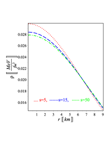
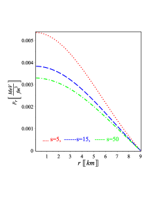
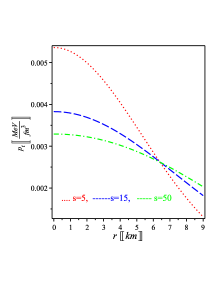
Figure 1: The energy density (left graph), the radial pressure (middle graph) and the tangential pressure (right graph) of the anisotropic star solution (III), as functions of the radial distance, for various values of the parameter $s$, using the 4U 1608-52 mass and radius values.

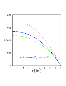
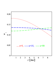
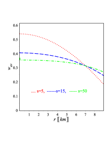
Figure 2: The radial equation-of-state parameter $w_{r}$ (left graph), the tangential equation-of-state parameter $w_{t}$ (middle graph) and the average equation-of-state parameter (right graph) of the anisotropic star solution (III), as functions of the radial distance, for various values of the parameter $s$, using the 4U 1608-52 mass and radius values.

In Fig. 2 we depict the radial, tangential, and average equation-of-state parameters, $w_{r}$, $w_{t}$ and $w_{av}$ respectively. As we observe $w_{r}$ is monotonically increasing and $w_{av}$ is monotonically decreasing with $r$, while $w_{t}$ is monotonically decreasing for small $s$ and monotonically increasing for large $s$. Moreover, the values of $w_{r}$, $w_{t}$ and $w_{av}$ are positive and lie in the interval $\{w_{t},\,\,w_{r},\,w_{av}\}\in[0,\,\,1]$, which implies that matter distribution is non-exotic in nature. Finally, in the left graph of Fig. 3 we depict the anisotropy $\Delta$, where we can see that it is positive, it vanishes at the center and it increases towards the surface of the star. Moreover, in the right graph of Fig. 3 we depict the anisotropic force $\frac{\Delta}{r}$, and the fact that it is positive implies that it is repulsive.

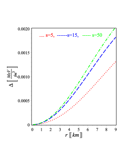
Figure 3: The anisotropy $\Delta$ (left graph), and the anisotropic force $\frac{\Delta}{r}$ (right graph) of the anisotropic star solution (III), as functions of the radial distance, for various values of the parameter $s$, using the 4U 1608-52 mass and radius values.

We proceed by investigating the behavior of the metric potentials. In Fig. 4 we present the temporal and the spatial components, for various choices of the model parameters. Furthermore, for transparency we additionally depict the smooth matching of the temporal component with the Schwarzschild exterior solution. As Fig. 4 shows, the metric potentials are both finite and positive at the center.

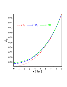
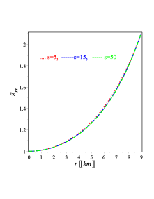
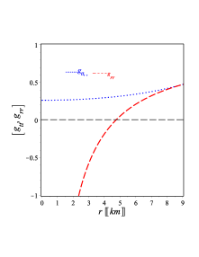
Figure 4: The temporal component (left graph) and the spatial component (middle graph) of the metric of the anisotropic solution (20), as functions of the radial distance, for various values of the parameter $s$, using the 4U 1608-52 mass and radius values. In the right graph we present the smooth matching of the temporal component with the Schwarzschild exterior solution.

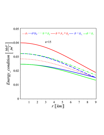
Figure 5: The Weak, Null, Strong and Dominant energy conditions of the anisotropic star solution (III), as functions of the radial distance, for $s=15$, using the 4U 1608-52 mass and radius values.

In Fig. 5 we depict the Weak, Null, Strong and Dominant energy conditions for $s=15$, showing that they obtain positive values and thus are all satisfied, as required for a physically meaningful stellar model (for other values of $s$ we obtain similar graphs).

In the left and middle graphs of Fig. 6 we present the radial and tangential sound speed squares, which indeed are positive and sub-luminal. Additionally, since a potentially stable configuration requires $v_{t}{}^{2}-v_{r}{}^{2}<0$ Herrera:1992lwz ; Boehmer:2006ye , in the right graph of Fig. 6 we depict the stability factor $v_{t}{}^{2}-v_{r}{}^{2}$, and as we see it is negative and hence we conclude that our model is potentially stable everywhere within the stellar interior for various values of the parameter $s$.

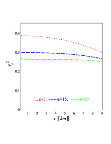
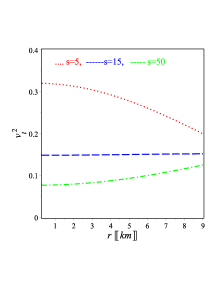
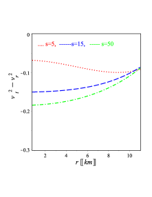
Figure 6: The radial sound speed square $v_{r}^{2}$ (left graph), the tangentiall sound speed square $v_{t}^{2}$ (middle graph) and the stability factor $v_{t}{}^{2}-v_{r}{}^{2}$ (right graph) of the anisotropic star solution (III), as functions of the radial distance, for various values of the parameter $s$, using the 4U 1608-52 mass and radius values.

The mass function given by (27) is plotted in the left graph of Fig. 7, showing that it is a monotonically increasing function of the radial coordinate and $M(r\rightarrow 0)=0$. Furthermore, the middle graph of Fig. 7 shows the behavior of the compactness parameter (28), which is increasing. Finally, the radial variation of the redshift (35) is plotted in the right graph of Fig. 7. We find that the surface redshift $Z_{R}\approx 0.45$ for all $s$ choices, and since the theoretical requirement is $Z_{R}\leq 2$ Buchdahl:1959zz we conclude that it is satisfied for solution (III).

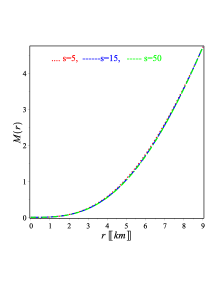
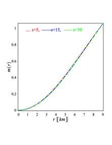
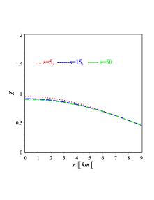
Figure 7: The mass $M(r)$ of (27) (left graph), the compactness $m(r)$ of (28) (middle graph) and the redshift (35) (right graph) of the anisotropic star solution (III), as functions of the radial distance, for various values of the parameter $s$, using the 4U 1608-52 mass and radius values. The surface redshift is $Z_{R}\approx 0.45$ for all $s$ choices.

V Stability

In this section, we are going to discuss the stability issue using two different techniques; the Tolman-Oppenheimer-Volkoff (TOV) equations and the adiabatic index. For completeness, we will also examine the static case, too.

V.1 Equilibrium analysis through TOV equation

In this subsection we are going to discuss the stability of a general stellar model. For this goal we assume hydrostatic equilibrium through the TOV equation. Using the TOV equation Tolman:1939jz ; Oppenheimer:1939ne as presented in 1993GReGr..25.1123P , we obtain the following form:

$$\frac{2[p_{t}-p_{r}]}{r}-\frac{M_{g}(r)[\rho(r)+p_{r}]\sqrt{h}}{r}-\frac{dp_{r}}{r}=0\,.$$ (37)

Here $M_{g}(r)$ is the mass of the gravitational system at radius $r$, and is defined through the Tolman-Whittaker mass formula

$$M_{g}(r)=4\pi{\int_{0}}^{r}\Big{(}{T_{t}}^{t}-{T_{r}}^{r}-{T_{\theta}}^{\theta}-{T_{\phi}}^{\phi}\Big{)}r^{2}h_{1}\sqrt{h}dr=\frac{r(h\,h_{1})^{\prime}}{2h\sqrt{h_{1}}}\,.$$ (38)

Inserting (38) into (37) we find

$$\frac{2(p_{t}-p_{r})}{r}-\frac{dp_{r}}{dr}-\frac{(h\,h_{1})^{\prime}(\rho+p_{r})}{2\sqrt{h\,h_{1}}}=F_{g}+F_{a}+F_{h}=0\,,$$ (39)

where $F_{g}=-\frac{(h\,h_{1})^{\prime}(\rho+p_{r})}{2\sqrt{h\,h_{1}}}$, $F_{a}=\frac{2(p_{t}-p_{r})}{r}$, and $F_{h}=-\frac{dp_{r}}{dr}$ are the gravitational, anisotropic and hydrostatic forces, respectively. The behavior of the TOV equation for model (III) is shown in Fig. 8, in which the three different forces are plotted (for other values of $s$ we obtain similar graphs). As we observe, the hydrostatic and anisotropic forces are positive, and are dominated by the gravitational force which is negative to maintain the system in static equilibrium.

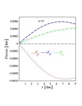
Figure 8: The gravitational, the anisotropic and the hydrostatic forces of the anisotropic star solution (III), as functions of the radial distance, for $s=15$, using the 4U 1608-52 mass and radius values.

V.2 Adiabatic index

The stable equilibrium configuration of a spherically symmetric system can be studied using the adiabatic index, which is a basic ingredient of the stability criterion. Considering an adiabatic perturbation, the adiabatic index $\Gamma$ is defined as Chandrasekhar:1964zz ; Merafina:2014goa ; 1989A&A…221….4M ; 1993MNRAS.265..533C :

$$\Gamma=\left(\frac{\rho+p}{p}\right)\left(\frac{dp}{d\rho}\right)\,.$$ (40)

A Newtonian isotropic sphere is in stable equilibrium if the adiabatic index satisfies $\Gamma>\frac{4}{3}$ 1975A&A….38…51H , while for $\Gamma=\frac{4}{3}$ the isotropic sphere is in neutral equilibrium. As it was shown in 1993MNRAS.265..533C , for the stability of a relativistic anisotropic sphere it is required that $\Gamma>\gamma$, where

$$\gamma=\frac{4}{3}-\left[\frac{4(p_{r}-p_{t})}{3\lvert p^{\prime}_{r}\lvert}\right]_{max}\,.$$ (41)

Using Eq. (40) and the solution (III), we can find the expressions for the radial and tangential adiabatic indices, which are presented in Appendix C.

In Fig. 9 we draw $\Gamma_{r}$ and $\Gamma_{t}$ for various values of $s$. As we can see, the profile of the radial and tangential adiabatic indices are monotonic increasing functions of $r$ and acquire values greater than $4/3$ everywhere within the stellar configuration for $s\leq 10$, thus the condition of stability is satisfied.

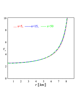
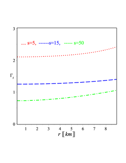
Figure 9: The radial adiabatic index (C) (left graph) and the tangential adiabatic index (C) (right graph), versus the radius $r$, for various values of $s$, using the 4U 1608-52 mass and radius values.

V.3 Stability in the static state

For completeness, in this subsection we discuss the stability in the static case. For a stable compact star, using the mass-central and mass-radius expression, as well as the relations for the energy density, Harrison, Zeldovich, and Novikov 1965gtgc.book…..H ; 1971reas.book…..Z stated that the gradient of the central density with respect to the mass, should acquire positive values, namely $\frac{\partial M}{\partial\rho_{r_{0}}}>0$, in order to have stable configurations. More precisely, the stable or unstable region is satisfied for constant mass, namely $\frac{\partial M}{\partial\rho_{r_{0}}}=0$ NewtonSingh:2019bbm .

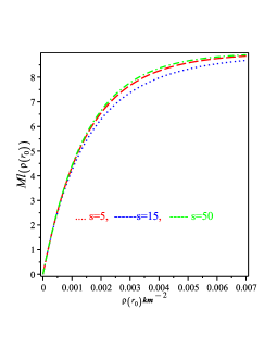
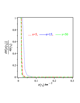
Figure 10: The mass (42) (left graph) and the mass gradient (43) (right graph), as functions of the central density $\rho_{r_{0}}$ for various values of $s$, using the 4U 1608-52 mass and radius values..

Let us apply this procedure to our solution (III). In this case, the central density becomes $\rho_{{}_{r_{0}}}=\frac{3s}{\kappa^{2}k^{2}}$ and thus we find that

$$M(\rho_{{}_{r_{0}}})=l\left[1-\left(1+\frac{\kappa^{2}l^{2}\rho_{r_{0}}}{3s}\right)^{-s}\right]\,,$$ (42)

which finally leads to

$$\frac{\partial M}{\partial\rho_{r_{0}}}=\frac{4\pi\,l^{3}\left(1+\frac{\kappa^{2}l^{2}\rho_{r_{0}}}{3s}\right)^{-s-1}}{3}\,.$$ (43)

The above expression implies that the solution (III) corresponds to a stable configuration since $\frac{\partial M}{\partial\rho_{r_{0}}}>0$ NewtonSingh:2019bbm . The behaviors of the mass and its gradient are shown in Fig. 10, and as we observe the mass decreases while the gradient-of-mass increases, as the energy density become smaller.

VI Discussion and conclusions

Mimetic gravity is an interesting modification obtained from general relativity through the isolation of the conformal degree of freedom in a covariant way, by applying a re-parametrization of the physical metric in terms of a mimetic field and an auxiliary metric. The present work aimed to investigate new anisotropic compact solutions within mimetic gravity, since such solutions are known to be very interesting laboratories of gravity in the strong-field regime.

We derived new classes of anisotropic solutions, by applying the Tolman-Finch-Skea metric, and a specific anisotropy not directly depending on it. Thus, the anisotropy is positive, it vanishes at the center of the star and it has no singularities. Additionally, we determined the involved integration constants by matching smoothly the interior anisotropic solution to the Schwarzschild exterior one, requiring additionally that the pressure must be vanishing at the boundary of the star.

In order to provide a transparent picture, we used the data from the 4U 1608-52 pulsar and we investigated numerically the features of the obtained anisotropic stars. In particular, we studied the profile of the energy density, as well as the radial and tangential pressures, and we showed that they are all positive and decrease towards the center of the star. Furthermore, we investigated the anisotropy parameter and the anisotropic force, which are both increasing functions of the radius, which implies that the latter is repulsive. Additionally, by examining the radial and tangential equation-of-state parameters, we showed that they are monotonically increasing, and bounded in the interval [0,1], which implies that the matter in our star is not exotic.

Concerning the metric potentials we saw that they have no singularity, either at the center of the star or at the boundary, and the matching to the Schwarzschild exterior is indeed smooth. Moreover, we examined the weak, null, strong and dominant energy conditions, showing that they are all satisfied in the interior of the star. Additionally, we examined the radial and tangential sound speed squares, showing that they are positive and sub-luminal, while we found that the surface redshift satisfies the requirement $Z_{R}\leq 2$. Finally, we provided the profiles for the mass and compactness, which are monotonically increasing functions of the radius.

In order to investigate the stability of the new anisotropic solutions, we applied the Tolman-Oppenheimer-Volkoff (TOV) equation, we performed the adiabatic index analysis, and we examined the static case, providing the profiles of the gravitational, anisotropic and hydrostatic forces of the star, the radial and tangential adiabatic indices, as well as the mass and its gradient, showing that in all cases the star is stable. Lastly, for completeness in the Appendix we provided the results for other pulsar data.

We mention that the obtained solutions do not have a trivial profile for the mimetic field, and therefore they correspond to novel classes, that do not exist for general relativity. Hence, the rich behavior of the aforementioned anisotropic solutions serves as an advantage of mimetic gravity. It would be interesting to investigate the gravitational wave structure of possible merges of such solutions, and whether this could provide signatures of mimetic gravity. Such an analysis will be performed in a future project.

Appendix A The radial and tangential sound speeds

The radial and tangential sound speed squares can be extracted from (III) as

$$\!\!\!\!\!\!\!\!\!\!\!\!\!v_{r}{}^{2}=\frac{dp_{r}}{d\rho}=\Bigg{\{}4({k}^{2}\!+\!{r}^{2})^{2}{c_{1}}^{2}\left[5(1\!+\!s)-({k}^{2}\!+\!{r}^{2})^{2+s}k^{-2s}{r}^{4}+{k}^{2}(s\!+\!2){r}^{2}\!+\!{k}^{4}\right]\left[({k}^{2}\!+\!{r}^{2})(s\!+\!2)\right]^{-s}$$

$$\ \ \ \ \ \ \ \ \ \ \ \ \ \ +(s\!-\!2)c_{1}\,c_{2}\left[2({k}^{2}\!+\!r^{2})^{2+s}k^{-2s}-(2+s^{2}+12s){r}^{4}-2{k}^{2}(s\!+\!2){r}^{2}-2{k}^{4}\right]$$

$$\ \ \ \ \ \ \ \ \ \ \ \ \ \ \ \ \,\ \cdot{2}^{s/2}({k}^{2}\!+\!{r}^{2})\left[({k}^{2}\!+\!{r}^{2})(s\!+\!2)\right]^{-s/2}$$

$$\ \ \ \ \ \ \ \ \ \ \ \ \ \ +(2\!-\!s)^{2}{c_{2}}^{2}\Bigg{[}({k}^{2}\!+\!{r}^{2})^{2}\left({\frac{{k}^{2}\!+\!{r}^{2}}{{k}^{2}}}\right)^{s}+(-2{s}^{2}\!-\!3s\!-\!1){r}^{4}-{k}^{2}(s\!+\!2){r}^{2}\!-\!{k}^{4}\Bigg{]}\Bigg{\}}$$

$$\ \ \ \ \ \ \ \ \ \ \ \ \ \ \cdot\Bigg{\{}\left\{c_{1}\,{2}^{1/2\,s}({k}^{2}\!+\!{r}^{2})\left[({k}^{2}\!+\!{r}^{2})(s\!+\!2)\right]^{-1/2\,s}-c_{2}(s\!-\!2)\right\}^{2}$$

$$\ \ \ \ \ \ \ \ \ \ \ \ \ \ \ \ \ \cdot\left[({k}^{2}\!+\!{r}^{2})^{2}\left({\frac{{k}^{2}+{r}^{2}}{{k}^{2}}}\right)^{s}+(-1\!+\!s\!+\!2{s}^{2}){r}^{4}-{k}^{2}(s\!+\!2){r}^{2}-{k}^{4}\right]\Bigg{\}}^{-1}\,,$$ (44)

$s$		$k\$ (km2)			$(c_{1})^{\frac{1}{s-2}}\$ (km)			$c_{2}$
1		$15.09$			$161$			$1.207$
$5$		$38.263$			$133$			$0.597$
$15$		$67.619$			$268$			$0.717$
$20$		$78.273$			$335$			$0.727$
$30$		$96.104$			$466$			$0.737$
$40$		$111.11$			$633$			$0.741$
$50$		$124.316$			$724$			$0.744$
$60$		$136.249$			$852$			$0.746$
$70$		$147.218$			$980$			$0.747$
$80$		$157.425$			$1107$			$0.748$
$90$		$167.009$			$1234$			$0.748$
$100$		$176.072$			$1361$			$0.749$

Table 1: The values of the constants $k,\,c_{1}$ and $c_{2}$ of (30)-(32), using the compact star 4U 1724-207, whose observed mass and radius are $(1.81_{-0.37}^{+0.25})M_{\odot}$ and $12.2\pm 1.4$ km respectively Miller:2019cac .

$$\!\!\!\!\!\!\!\!\!\!\!\!\!\!\!\!\!\!\!\!\!\!\!\!\!\!v_{t}{}^{2}=\frac{dp_{t}}{d\rho}={r}^{4}\Bigg{\{}({k}^{2}\!+\!{r}^{2})^{2}{c_{1}}^{2}\left[({k}^{2}\!+\!3\,{r}^{2}){s}^{2}+(-5{k}^{2}\!-\!{r}^{2})s-4{k}^{2}\!-\!4{r}^{2}\right]{2}^{s}\left[({k}^{2}\!+\!{r}^{2})(s\!+\!2)\right]^{-s}$$

$$\ \ \ \ \ \ \ \ +c_{1}\,c_{2}\,\left(2-s\right)({k}^{2}\!+\!{r}^{2})\left[({k}^{2}\!+\!5{r}^{2})s-12{k}^{2}-4{r}^{2}\right]{2}^{1/2s}s\left[({k}^{2}\!+\!{r}^{2})(s\!+\!2)\right]^{-1/2s}$$

$$\ \ \ \ \ \ \ \ -(s\!-\!2)^{2}{c_{2}}^{2}\left[({k}^{2}\!-\!{r}^{2})s-{r}^{2}+3{k}^{2}\right]s\Bigg{\}}$$

$$\ \ \ \cdot\Bigg{\{}({k}^{2}\!+\!{r}^{2})\left\{\left[({k}^{2}\!+\!{r}^{2})^{2}-{k}^{2}+{r}^{2}\right]^{2+s}k^{-2s}-r^{2}({r}^{2}\!-\!{k}^{2})s\right\}$$

$$\ \ \ \cdot\left\{c_{1}\,{2}^{s/2}({k}^{2}\!+\!{r}^{2})\left[({k}^{2}\!+\!{r}^{2})(s\!+\!2)\right]^{-s/2}+c_{2}(2\!-\!s)\right\}^{2}\Bigg{\}}^{-1}\,.$$ (45)

s		$\rho\lvert_{{}_{{}_{0}}}$		$\rho\lvert_{{}_{{}_{l}}}$		$\frac{dp_{r}}{d\rho}\lvert_{{}_{{}_{0}}}$		$\frac{dp_{r}}{d\rho}\lvert_{{}_{{}_{l}}}$		$\frac{dp_{t}}{d\rho}\lvert_{{}_{{}_{0}}}$		$\frac{dp_{t}}{d\rho}\lvert_{{}_{{}_{l}}}$		$\Gamma_{r}\lvert_{{}_{{}_{0}}}$		$\Gamma_{t}\lvert_{{}_{{}_{0}}}$
$1$		$0.0132$		$0.005$		$0.56$		$0.33$		$0.76$		$0.179$		$2.5$		$3.4$
$5$		$0.01$		$0.0057$		$0.413$		$0.343$		$0.346$		$0.245$		$2.82$		$2.25$
$15$		$0.0098$		$0.0059$		$0.247$		$0.228$		$0.097$		$0.105$		$2.82$		$1.11$
$20$		$0.0097$		$0.0059$		$0.235$		$0.222$		$0.074$		$0.094$		$2.81$		$0.88$
$30$		$0.0097$		$0.0059$		$0.233$		$0.217$		$0.049$		$0.083$		$2.8$		$0.62$
$40$		$0.0097$		$0.0059$		$0.217$		$0.214$		$0.037$		$0.077$		$2.8$		$0.47$
$50$		$0.0097$		$0.0059$		$0.213$		$0.212$		$0.029$		$0.073$		$2.8$		$0.38$
$60$		$0.0097$		$0.0059$		$0.211$		$0.21$		$0.024$		$0.07$		$2.8$		$0.3$
$70$		$0.0097$		$0.0059$		$0.21$		$0.21$		$0.02$		$0.069$		$2.8$		$0.27$
$80$		$0.0097$		$0.0059$		$0.21$		$0.21$		$0.017$		$0.068$		$2.8$		$0.2$
$90$		$0.0097$		$0.0059$		$0.21$		$0.21$		$0.015$		$0.066$		$2.8$		$0.2$
$100$		$0.0097$		$0.0059$		$0.21$		$0.21$		$0.014$		$0.065$		$2.8$		$0.18$

Table 2: Numerical values of physical quantities of the anisotropic star solution (III), for various values of the parameter $s$, using the 4U 1724-207 mass and radius values. The energy density is measured in MeV$\cdot$fm^-3, while all other quantifies are dimensionless in units where $c=1$.

Appendix B Analysis using 4U 1724-207 and J0030+0451 pulsars

In addition to 4U 1608-52, a similar analysis can be developed for other pulsars. In particular, using the pulsar 4U 1724-207, whose observed mass and radius given by $(1.81_{-0.37}^{+0.25})M_{\odot}$ and $12.2\pm 1.4$ km respectively Miller:2019cac , we obtain the model parameters displayed in Table 1, and using them we obtain the physical quantities summarized in Table 2.

Additionally, in Table 3 we display the corresponding parameters for the pulsar J0030+0451, whose observed mass and radius is given by $(1.34_{-0.16}^{+0.15})M_{\odot}$ and $12.71_{-1.19}^{+1.14}$ km respectively Riley:2019yda , and using them we obtain the physical quantities summarized in Table 4.

$s$		$k\$ (km2)			$(c_{1})^{\frac{1}{s-2}}\$ (km)			$c_{2}$
1		$17.46$			$43$			$1.787$
$5$		$42.086$			$171$			$0.521$
$15$		$73.786$			$302$			$0.767$
$20$		$85.33$			$373$			$0.786$
$30$		$104.665$			$514$			$0.805$
$40$		$120.948$			$654$			$0.814$
$50$		$135.285$			$794$			$0.819$
$60$		$148.242$			$933$			$0.823$
$70$		$160.154$			$1072$			$0.825$
$80$		$171.239$			$1210$			$0.827$
$90$		$181.65$			$1348$			$0.828$
$100$		$191.495$			$1486$			$0.83$

Table 3: The values of the constants $k,\,c_{1}$ and $c_{2}$ of (30)-(32), using the compact star J0030+0451, whose observed mass and radius are $(1.34_{-0.16}^{+0.15})M_{\odot}$ and $12.71_{-1.19}^{+1.14}$ km respectively Riley:2019yda .

s		$\rho\lvert_{{}_{{}_{0}}}$		$\rho\lvert_{{}_{{}_{l}}}$		$\frac{dp_{r}}{d\rho}\lvert_{{}_{{}_{0}}}$		$\frac{dp_{r}}{d\rho}\lvert_{{}_{{}_{l}}}$		$\frac{dp_{t}}{d\rho}\lvert_{{}_{{}_{0}}}$		$\frac{dp_{t}}{d\rho}\lvert_{{}_{{}_{l}}}$		$\Gamma_{r}\lvert_{{}_{{}_{0}}}$		$\Gamma_{t}\lvert_{{}_{{}_{0}}}$
$1$		$0.0098$		$0.006$		$0.475$		$0.331$		$0.675$		$0.26$		$3.07$		$4.36$
$5$		$0.0085$		$0.006$		$0.26$		$0.23$		$0.193$		$0.134$		$3.83$		$2.85$
$15$		$0.0083$		$0.006$		$0.19$		$0.182$		$0.04$		$0.046$		$3.96$		$0.837$
$20$		$0.0082$		$0.006$		$0.18$		$0.176$		$0.018$		$0.032$		$3.96$		$0.4$
$30$		$0.0082$		$0.006$		$0.17$		$0.169$		$-0.0044$		$0.0178$		$3.97$		$-0.103$
$40$		$0.0082$		$0.006$		$0.164$		$0.166$		$-0.016$		$0.01$		$3.97$		$-0.386$
$50$		$0.0082$		$0.006$		$0.161$		$0.164$		$-0.023$		$0.0056$		$3.97$		$-0.567$
$60$		$0.0082$		$0.006$		$0.159$		$0.163$		$-0.028$		$0.003$		$3.97$		$-0.7$
$70$		$0.0082$		$0.006$		$0.158$		$0.162$		$-0.031$		$0.0002$		$3.97$		$-0.79$
$80$		$0.0082$		$0.006$		$0.156$		$0.16$		$-0.034$		$-0.0015$		$3.97$		$-0.856$
$90$		$0.0082$		$0.006$		$0.155$		$0.16$		$-0.036$		$-0.0028$		$3.97$		$-0.9$
$100$		$0.0082$		$0.006$		$0.155$		$0.16$		$-0.0374$		$-0.0039$		$3.96$		$-0.96$

Table 4: Numerical values of physical quantities of the anisotropic star solution (III), for various values of the parameter $s$, using the J0030+0451 mass and radius values. The energy density is measured in MeV$\cdot$fm^-3, while all other quantifies are dimensionless in units where $c=1$. Note that for increasing values of $s$, some quantities acquire nonphysical values, such as $\frac{dp_{t}}{d\rho}\lvert_{{}_{{}_{0}}}$, $\frac{dp_{t}}{d\rho}\lvert_{{}_{{}_{l}}}$ and $\Gamma_{t}\lvert_{{}_{{}_{0}}}$.

Appendix C The radial and tangential adiabatic index

The adiabatic index of a spherically symmetric system is defined as Chandrasekhar:1964zz ; 1989A&A…221….4M ; 1993MNRAS.265..533C :

$$\Gamma=\left(\frac{\rho+p}{p}\right)\left(\frac{dp}{d\rho}\right)\,,$$ (46)

and can be applied for the radial and tangential pressure separately. Hence, inserting the solution (III) into (40) we obtain the radial adiabatic index as

$$\!\!\!\!\Gamma_{r}=2{r}^{2}\left\{c_{1}\,{2}^{s/2}(k^{2}\!+\!{r}^{2})(s\!+\!2)\left[(k^{2}\!+\!{r}^{2})(s\!+\!2)\right]^{-1/2\,s}-2\,sc_{2}\,(s\!-\!2)\right\}$$

$$\ \ \ \ \ \ \ \cdot\Bigg{\{}(k^{2}\!+\!{r}^{2})^{2}\left({\frac{k^{2}\!+\!{r}^{2}}{k^{2}}}\right)^{s}+(s\!+\!2{s}^{2}\!-\!1){r}^{4}-k^{2}(s\!+\!2){r}^{2}-k^{4}\Bigg{\}}^{-1}$$

$$\ \ \ \ \ \ \ \cdot\Bigg{\{}s^{s}\left[(k^{2}\!+\!{r}^{2})^{2+s}k^{-2s}-5(s\!+\!1){r}^{4}-k^{2}(s\!+\!2){r}^{2}-k^{4}\right]{c_{1}}^{2}(k^{2}\!+\!{r}^{2})^{2}\left[(k^{2}\!+{\!r}^{2})(s\!+\!2)\right]^{-s}$$

$$\ \ \ \ \ \ \ \ \ \,\ -(s\!-\!2){2}^{s/2}\left[2(k^{2}\!+\!{r}^{2})^{2+s}k^{-2s}-({s}^{2}\!+\!12s+2){r}^{4}-2k^{4}-2k^{2}(s\!+\!2){r}^{2}\right]$$

$$\ \ \ \ \ \ \ \ \ \,\ \ \,\ \cdot c_{1}(k^{2}\!+\!{r}^{2})c_{2}\left[(k^{2}\!+\!{r}^{2})(s\!+\!2)\right]^{-s/2}$$

$$\ \ \ \ \ \ \ \ \ \,\ +(s\!-\!2)^{2}{c_{2}}^{2}\left[(k^{2}\!+\!{r}^{2})^{2+s}k^{-2s}-(2{s}^{2}\!+\!3s\!+\!1){r}^{4}-k^{4}-k^{2}(s\!+\!2){r}^{2}\right]\Bigg{\}}$$

$$\ \ \ \ \ \ \ \cdot\Bigg{\{}c_{1}(k^{2}\!+\!{r}^{2})\left[(k^{2}\!+\!{r}^{2})^{1+s}k^{-2s}\!-\!k^{2}\!-\!5{r}^{2}\right]{2}^{s/2}\left[(k^{2}\!+\!{r}^{2})(s\!+\!2)\right]^{-s/2}$$

$$\ \ \ \ \ \ \ \ \ -c_{2}\Bigg{[}(k^{2}\!+\!{r}^{2})^{1+s}k^{-2s}+(-2s-1){r}^{2}\!-\!k^{2}\Bigg{]}(s\!-\!2)\Bigg{\}}^{-1}$$

$$\ \ \ \ \ \ \ \cdot\Bigg{\{}c_{1}\,{2}^{s/2}(k^{2}\!+\!{r}^{2})\left[(k^{2}\!+\!{r}^{2})(s\!+\!2)\right]^{-1/2\,s}-c_{2}(s\!-\!2)\Bigg{\}}^{-2}\,,$$ (47)

and the tangential adiabatic index as

$$\!\!\!\!\!\!\!\!\!\!\!\!\!\!\Gamma_{t}={r}^{2}\Bigg{\{}4{c_{1}}^{2}\left[(3{s}^{2}\!-\!4\!-\!s){r}^{2}+(s^{2}\!-\!5s\!-\!4){k}^{2}\right]({k}^{2}\!+\!{r}^{2})^{2}\left[({k}^{2}\!+\!{r}^{2})(s\!+\!2)\right]^{-s}$$

$$\ \ \ \ \ -c_{2}\,{2}^{s/2}s(s\!-\!2)c_{1}({k}^{2}\!+\!{r}^{2})\left[(5s\!-4\!){r}^{2}+{k}^{2}(s\!-\!12)\right]\left[({k}^{2}\!+\!{r}^{2})(s\!+\!2)\right]^{-s/2}$$

$$\ \ \ \ \ -{c_{2}}^{2}s\left(s-2\right)^{2}\left[{k}^{2}(s\!+\!3)-(s\!+\!1){r}^{2}\right]\Bigg{\}}$$

$$\cdot\Bigg{\{}{2}^{s/2}c_{1}\left[({k}^{2\!}+\!{r}^{2})^{2+s}k^{-2s}+(3-s){r}^{4}+{k}^{2}(s\!+\!2){r}^{2}-{k}^{4}\right]$$

$$\ \ \ \cdot({k}^{2}\!+\!{r}^{2})\left[({k}^{2}\!+\!{r}^{2})(s\!+\!2)\right]^{-s/2}$$

$$\ \ \ \,-c_{2}(s\!-\!2)\left[({k}^{2}\!+\!{r}^{2})^{2+s}k^{-2s}+(s\!-\!1){r}^{4}+(3s\!-\!2){k}^{2}{r}^{2}\!-\!{k}^{4}\right]\Bigg{\}}$$

$$\cdot\Bigg{\{}\left[({k}^{2}\!+\!{r}^{2})^{2+s}k^{-2s}\!+\!(s\!-\!1\!+\!2{s}^{2}){r}^{4}\!-\!{k}^{2}(s\!+\!2){r}^{2}\!-\!{k}^{4}\right]$$

$$\ \ \ \cdot({k}^{2}\!+\!{r}^{2})\left\{c_{1}\,{2}^{1/2\,s}({k}^{2}\!+\!{r}^{2})\left[({k}^{2}\!+\!{r}^{2})(s\!+\!2)\right]^{-1/2s}-c_{2}(s\!-\!2)\right\}$$

$$\cdot\left\{\left[(3s\!-\!4){r}^{2}+(s\!-\!4){k}^{2}\right]{2}^{1/2\,s}c_{1}\,\left({k}^{2}+{r}^{2}\right)\left[({k}^{2}\!+\!{r}^{2})(s\!+\!2)\right]^{-1/2s}\right.$$

$$\left.\ \ \ \ +sc_{2}(k\!-\!r)(k\!+\!r)(s\!-\!2)\right\}\Bigg{\}}^{-1}\,.$$ (48)

Data Availability Statement

No Data associated in the manuscript.

References

- (1) T. Damour and G. Esposito-Farese, Tensor - scalar gravity and binary pulsar experiments, Phys. Rev. D 54, 1474-1491 (1996) [arXiv:gr-qc/9602056].
- (2) C. M. Will, The Confrontation between General Relativity and Experiment, Living Rev. Rel. 17, 4 (2014) [arXiv:1403.7377].
- (3) E. Berti, E. Barausse, V. Cardoso, L. Gualtieri, P. Pani, U. Sperhake, L. C. Stein, N. Wex, K. Yagi and T. Baker, et al. Testing General Relativity with Present and Future Astrophysical Observations, Class. Quant. Grav. 32, 243001 (2015) [arXiv:1501.07274].
- (4) B. P. Abbott et al. [LIGO Scientific and Virgo], Tests of general relativity with GW150914, Phys. Rev. Lett. 116, no.22, 221101 (2016) [erratum: Phys. Rev. Lett. 121, no.12, 129902 (2018)] [arXiv:1602.03841].
- (5) E. Berti, K. Yagi and N. Yunes, Extreme Gravity Tests with Gravitational Waves from Compact Binary Coalescences: (I) Inspiral-Merger, Gen. Rel. Grav. 50, no.4, 46 (2018) [arXiv:1801.03208].
- (6) A. De Felice and S. Tsujikawa, f(R) theories, Living Rev. Rel. 13, 3 (2010) [arXiv:1002.4928].
- (7) I. Antoniadis, J. Rizos and K. Tamvakis, Singularity - free cosmological solutions of the superstring effective action, Nucl. Phys. B 415, 497 (1994).
- (8) S. ’i. Nojiri and S. D. Odintsov, Modified Gauss-Bonnet theory as gravitational alternative for dark energy, Phys. Lett. B 631, 1 (2005) [arXiv:hep-th/0508049].
- (9) P. D. Mannheim and D. Kazanas, Exact Vacuum Solution to Conformal Weyl Gravity and Galactic Rotation Curves, Astrophys. J. 342, 635 (1989).
- (10) D. Lovelock, The Einstein tensor and its generalizations, J. Math. Phys. 12, 498 (1971).
- (11) N. Deruelle and L. Farina-Busto, The Lovelock Gravitational Field Equations in Cosmology, Phys. Rev. D 41, 3696 (1990).
- (12) M. Fierz, On the physical interpretation of P.Jordan’s extended theory of gravitation, Helv. Phys. Acta 29, 128-134 (1956).
- (13) P. Jordan, The present state of Dirac’s cosmological hypothesis, Z. Phys. 157, 112-121 (1959).
- (14) C. Brans and R. H. Dicke, Mach’s principle and a relativistic theory of gravitation, Phys. Rev. 124, 925-935 (1961).
- (15) T. Damour and G. Esposito-Farese, Tensor multiscalar theories of gravitation, Class. Quant. Grav. 9, 2093-2176 (1992).
- (16) E. N. Saridakis et al. [CANTATA], Modified Gravity and Cosmology: An Update by the CANTATA Network, [arXiv:2105.12582].
- (17) G. R. Bengochea and R. Ferraro, Dark torsion as the cosmic speed-up, Phys. Rev. D 79, 124019 (2009) [arXiv:0812.1205].
- (18) Y. F. Cai, S. Capozziello, M. De Laurentis and E. N. Saridakis, f(T) teleparallel gravity and cosmology, Rept. Prog. Phys. 79, no.10, 106901 (2016) [arXiv:1511.07586].
- (19) G. Kofinas and E. N. Saridakis, Teleparallel equivalent of Gauss-Bonnet gravity and its modifications, Phys. Rev. D 90, 084044 (2014) [arXiv:1404.2249].
- (20) C. Q. Geng, C. C. Lee, E. N. Saridakis and Y. P. Wu, “Teleparallel” dark energy, Phys. Lett. B 704, 384-387 (2011) [arXiv:1109.1092].
- (21) D. Garfinkle, G. T. Horowitz and A. Strominger, Charged black holes in string theory, Phys. Rev. D 43, 3140 (1991) [erratum: Phys. Rev. D 45, 3888 (1992)].
- (22) P. Kanti, N. E. Mavromatos, J. Rizos, K. Tamvakis and E. Winstanley, Dilatonic black holes in higher curvature string gravity, Phys. Rev. D 54, 5049-5058 (1996) [arXiv:hep-th/9511071].
- (23) R. G. Cai, Gauss-Bonnet black holes in AdS spaces, Phys. Rev. D 65, 084014 (2002) [arXiv:hep-th/0109133].
- (24) P. Kanti, Black holes in theories with large extra dimensions: A Review, Int. J. Mod. Phys. A 19, 4899-4951 (2004) [arXiv:hep-ph/0402168].
- (25) R. Emparan and H. S. Reall, Black Holes in Higher Dimensions, Living Rev. Rel. 11, 6 (2008) [arXiv:0801.3471].
- (26) S. Nojiri and S. D. Odintsov, Phys. Rept. 505 (2011), 59-144 doi:10.1016/j.physrep.2011.04.001 [arXiv:1011.0544 [gr-qc]].
- (27) E. B. Kiritsis and G. Kofinas, On Horava-Lifshitz ’Black Holes’, JHEP 01, 122 (2010) [arXiv:0910.5487].
- (28) P. Pani, V. Cardoso and T. Delsate, Compact stars in Eddington inspired gravity, Phys. Rev. Lett. 107, 031101 (2011) [arXiv:1106.3569].
- (29) P. A. Gonzalez, E. N. Saridakis and Y. Vasquez, Circularly symmetric solutions in three-dimensional Teleparallel, f(T) and Maxwell-f(T) gravity, JHEP 07, 053 (2012) [arXiv:1110.4024].
- (30) P. Pani, E. Berti, V. Cardoso and J. Read, Compact stars in alternative theories of gravity. Einstein-Dilaton-Gauss-Bonnet gravity, Phys. Rev. D 84, 104035 (2011) [arXiv:1109.0928].
- (31) S. Capozziello, P. A. Gonzalez, E. N. Saridakis and Y. Vasquez, Exact charged black-hole solutions in D-dimensional f(T) gravity: torsion vs curvature analysis, JHEP 02, 039 (2013) [arXiv:1210.1098].
- (32) S. Nojiri, S. D. Odintsov and V. K. Oikonomou, Phys. Rept. 692 (2017), 1-104 doi:10.1016/j.physrep.2017.06.001 [arXiv:1705.11098 [gr-qc]].
- (33) Y. F. Cai, D. A. Easson, C. Gao and E. N. Saridakis, Charged black holes in nonlinear massive gravity, Phys. Rev. D 87, 064001 (2013) [arXiv:1211.0563].
- (34) G. G. L. Nashed, Spherically symmetric charged-dS solution in gravity theories, Phys. Rev. D 88, 104034 (2013) [arXiv:1311.3131].
- (35) A. V. Astashenok and S. D. Odintsov, Phys. Rev. D 94 (2016) no.6, 063008 doi:10.1103/PhysRevD.94.063008 [arXiv:1512.07279 [gr-qc]].
- (36) A. Anabalon, A. Cisterna and J. Oliva, Asymptotically locally AdS and flat black holes in Horndeski theory, Phys. Rev. D 89, 084050 (2014) [arXiv:1312.3597].
- (37) R. Garattini and E. N. Saridakis, Gravity’s Rainbow: a bridge towards Hořava–Lifshitz gravity, Eur. Phys. J. C 75, no.7, 343 (2015) [arXiv:1411.7257].
- (38) A. Cisterna and C. Erices, Asymptotically locally AdS and flat black holes in the presence of an electric field in the Horndeski scenario, Phys. Rev. D 89, 084038 (2014) [arXiv:1401.4479].
- (39) A. Paliathanasis, S. Basilakos, E. N. Saridakis, S. Capozziello, K. Atazadeh, F. Darabi and M. Tsamparlis, New Schwarzschild-like solutions in f(T) gravity through Noether symmetries, Phys. Rev. D 89, 104042 (2014) [arXiv:1402.5935].
- (40) H. Lu, A. Perkins, C. N. Pope and K. S. Stelle, Black Holes in Higher-Derivative Gravity, Phys. Rev. Lett. 114, no.17, 171601 (2015) [arXiv:1502.01028].
- (41) E. Babichev, C. Charmousis and M. Hassaine, Charged Galileon black holes, JCAP 05, 031 (2015) [arXiv:1503.02545].
- (42) P. H. R. S. Moraes, J. D. V. Arbañil and M. Malheiro, Stellar equilibrium configurations of compact stars in gravity, JCAP 06, 005 (2016) [arXiv:1511.06282].
- (43) A. V. Astashenok, S. D. Odintsov and V. K. Oikonomou, Class. Quant. Grav. 32 (2015) no.18, 185007 doi:10.1088/0264-9381/32/18/185007 [arXiv:1504.04861 [gr-qc]].
- (44) C. Erices and C. Martinez, Rotating hairy black holes in arbitrary dimensions, Phys. Rev. D 97, no.2, 024034 (2018) [arXiv:1707.03483].
- (45) D. D. Doneva and G. Pappas, Universal Relations and Alternative Gravity Theories, Astrophys. Space Sci. Libr. 457, 737-806 (2018) [arXiv:1709.08046].
- (46) D. D. Doneva and S. S. Yazadjiev, New Gauss-Bonnet Black Holes with Curvature-Induced Scalarization in Extended Scalar-Tensor Theories, Phys. Rev. Lett. 120, no.13, 131103 (2018) [arXiv:1711.01187].
- (47) M. K. Jasim, D. Deb, S. Ray, Y. K. Gupta and S. R. Chowdhury, Anisotropic strange stars in Tolman–Kuchowicz spacetime, Eur. Phys. J. C 78, no.7, 603 (2018) [arXiv:1801.10594].
- (48) Z. Roupas, G. Panotopoulos and I. Lopes, QCD color superconductivity in compact stars: color-flavor locked quark star candidate for the gravitational-wave signal GW190814, Phys. Rev. D 103, no.8, 083015 (2021) [arXiv:2010.11020].
- (49) T. Karakasis, E. Papantonopoulos, Z. Y. Tang and B. Wang, Exact black hole solutions with a conformally coupled scalar field and dynamic Ricci curvature in f(R) gravity theories, Eur. Phys. J. C 81, no.10, 897 (2021) [arXiv:2103.14141].
- (50) G. G. L. Nashed, Rotating charged black hole spacetimes in quadratic f(R) gravitational theories, Int. J. Mod. Phys. D 27, no.7, 1850074 (2018)
- (51) X. Ren, Y. Zhao, E. N. Saridakis and Y. F. Cai, Deflection angle and lensing signature of covariant f(T) gravity, JCAP 10, 062 (2021) [arXiv:2105.04578].
- (52) G. G. L. Nashed and E. N. Saridakis, Rotating AdS black holes in Maxwell- gravity, Class. Quant. Grav. 36, no.13, 135005 (2019) [arXiv:1811.03658 [gr-qc]].
- (53) C. E. Mota, L. C. N. Santos, F. M. da Silva, C. V. Flores, T. J. N. da Silva and D. P. Menezes, Anisotropic compact stars in Rastall–Rainbow gravity, Class. Quant. Grav. 39, no.8, 085008 (2022).
- (54) S. Kiorpelidi, G. Koutsoumbas, A. Machattou and E. Papantonopoulos, Topological black holes with curvature induced scalarization in the extended scalar-tensor theories, Phys. Rev. D 105, no.10, 104039 (2022) [arXiv:2102.00655].
- (55) N. Chatzifotis, P. Dorlis, N. E. Mavromatos and E. Papantonopoulos, Scalarization of Chern-Simons-Kerr black hole solutions and wormholes, Phys. Rev. D 105, no.8, 084051 (2022) [arXiv:2102.03496].
- (56) Y. Zhao, X. Ren, A. Ilyas, E. N. Saridakis and Y. F. Cai, Quasinormal modes of black holes in gravity, [arXiv:2204.11169].
- (57) A. H. Chamseddine and V. Mukhanov, Mimetic Dark Matter, JHEP 1311, 135 (2013) [arXiv:1308.5410].
- (58) A. H. Chamseddine, V. Mukhanov and A. Vikman, Cosmology with Mimetic Matter, JCAP 1406, 017 (2014) [arXiv:1403.3961].
- (59) S. Nojiri and S. D. Odintsov, Mimetic gravity: inflation, dark energy and bounce, [arXiv:1408.3561].
- (60) D. Momeni, R. Myrzakulov and E. Güdekli, Cosmological viable mimetic and theories via Noether symmetry, Int. J. Geom. Meth. Mod. Phys. 12, no.10, 1550101 (2015) [arXiv:1502.00977].
- (61) J. Matsumoto, S. D. Odintsov and S. V. Sushkov, Cosmological perturbations in a mimetic matter model, Phys. Rev. D 91, no.6, 064062 (2015) [arXiv:1501.02149].
- (62) A. H. Chamseddine and V. Mukhanov, Resolving Cosmological Singularities, JCAP 03, 009 (2017) [arXiv:1612.05860].
- (63) A. H. Chamseddine and V. Mukhanov, Nonsingular Black Hole, Eur. Phys. J. C 77, no.3, 183 (2017) [arXiv:1612.05861].
- (64) A. Casalino, M. Rinaldi, L. Sebastiani and S. Vagnozzi, Mimicking dark matter and dark energy in a mimetic model compatible with GW170817, Phys. Dark Univ. 22, 108 (2018) [arXiv:1803.02620].
- (65) G. G. L. Nashed and S. Capozziello, Eur. Phys. J. C 81, no.5, 481 (2021) doi:10.1140/epjc/s10052-021-09273-8 [arXiv:2105.11975 [gr-qc]].
- (66) A. Casalino, M. Rinaldi, L. Sebastiani and S. Vagnozzi, Alive and well: mimetic gravity and a higher-order extension in light of GW170817, Class. Quant. Grav. 36, no.1, 017001 (2019) [arXiv:1811.06830].
- (67) S. Vagnozzi, Recovering a MOND-like acceleration law in mimetic gravity, Class. Quant. Grav. 34, no.18, 185006 (2017) [arXiv:1708.00603].
- (68) J. Dutta, W. Khyllep, E. N. Saridakis, N. Tamanini and S. Vagnozzi, Cosmological dynamics of mimetic gravity, JCAP 02, 041 (2018) [arXiv:1711.07290].
- (69) G. G. L. Nashed, Annalen Phys. 523, 450-458 (2011) doi:10.1002/andp.201100030 [arXiv:1105.0328 [gr-qc]].
- (70) M. H. Abbassi, A. Jozani and H. R. Sepangi, Anisotropic Mimetic Cosmology, Phys. Rev. D 97, no.12, 123510 (2018) [arXiv:1803.00209].
- (71) Y. Zhong and D. Sáez-Chillón Gómez, Inflation in mimetic gravity, Symmetry 10, no.5, 170 (2018) [arXiv:1805.03467].
- (72) G. G. L. Nashed and S. Capozziello, Eur. Phys. J. C 80, no.10, 969 (2020) doi:10.1140/epjc/s10052-020-08551-1 [arXiv:2010.06355 [gr-qc]].
- (73) S. D. Odintsov and V. K. Oikonomou, Accelerating cosmologies and the phase structure of F(R) gravity with Lagrange multiplier constraints: A mimetic approach, Phys. Rev. D 93, no.2, 023517 (2016) [arXiv:1511.04559].
- (74) S. Nojiri, S. D. Odintsov and V. K. Oikonomou, Viable Mimetic Completion of Unified Inflation-Dark Energy Evolution in Modified Gravity, Phys. Rev. D 94, no.10, 104050 (2016) [arXiv:1608.07806].
- (75) N. Sadeghnezhad and K. Nozari, Braneworld Mimetic Cosmology, Phys. Lett. B 769, 134-140 (2017) [arXiv:1703.06269].
- (76) M. A. Gorji, S. Mukohyama and H. Firouzjahi, Cosmology in Mimetic SU(2) Gauge Theory, JCAP 05, 019 (2019) [arXiv:1903.04845].
- (77) M. A. Gorji, S. Mukohyama, H. Firouzjahi and S. A. Hosseini Mansoori, Gauge Field Mimetic Cosmology, JCAP 08, 047 (2018) [arXiv:1807.06335].
- (78) W. El Hanafy and G. G. L. Nashed, Int. J. Mod. Phys. D 26, no.14, 1750154 (2017) doi:10.1142/S0218271817501541 [arXiv:1707.01802 [gr-qc]].
- (79) M. Bouhmadi-López, C. Y. Chen and P. Chen, Primordial Cosmology in Mimetic Born-Infeld Gravity, JCAP 11, 053 (2017) [arXiv:1709.09192].
- (80) M. A. Gorji, S. A. Hosseini Mansoori and H. Firouzjahi, Higher Derivative Mimetic Gravity, JCAP 01, 020 (2018) [arXiv:1709.09988].
- (81) H. Firouzjahi, M. A. Gorji, S. A. Hosseini Mansoori, A. Karami and T. Rostami, Two-field disformal transformation and mimetic cosmology, JCAP 11, 046 (2018) [arXiv:1806.11472].
- (82) A. H. Chamseddine, V. Mukhanov and T. B. Russ, Asymptotically Free Mimetic Gravity, Eur. Phys. J. C 79, no.7, 558 (2019) [arXiv:1905.01343].
- (83) G. G. L. Nashed, Anisotropic Compact Stars in the Mimetic Gravitational Theory, Astrophys. J. 919, no.2, 113 (2021) [arXiv:2108.04060].
- (84) G. Leon and E. N. Saridakis, Dynamical behavior in mimetic F(R) gravity, JCAP 04, 031 (2015) [arXiv:1501.00488].
- (85) G. G. L. Nashed and W. El Hanafy, Eur. Phys. J. C 77, no.2, 90 (2017) doi:10.1140/epjc/s10052-017-4663-6 [arXiv:1612.05106 [gr-qc]].
- (86) L. Sebastiani, S. Vagnozzi and R. Myrzakulov, Mimetic gravity: a review of recent developments and applications to cosmology and astrophysics, Adv. High Energy Phys. 2017, 3156915 (2017) [arXiv:1612.08661].
- (87) E. Abdalla, G. Franco Abellán, A. Aboubrahim, A. Agnello, et al. Cosmology intertwined: A review of the particle physics, astrophysics, and cosmology associated with the cosmological tensions and anomalies, JHEAp 34, 49 (2022) [arXiv:2203.06142].
- (88) A. Addazi, J. Alvarez-Muniz, R. Alves Batista, G. Amelino-Camelia, et al. Quantum gravity phenomenology at the dawn of the multi-messenger era—A review, Prog. Part. Nucl. Phys. 125, 103948 (2022) [arXiv:2111.05659].
- (89) N. Deruelle and J. Rua, Disformal Transformations, Veiled General Relativity and Mimetic Gravity, JCAP 09, 002 (2014) [arXiv:1407.0825].
- (90) R. Myrzakulov and L. Sebastiani, Spherically symmetric static vacuum solutions in Mimetic gravity, Gen. Rel. Grav. 47, no.8, 89 (2015) [arXiv:1503.04293].
- (91) R. Myrzakulov, L. Sebastiani, S. Vagnozzi and S. Zerbini, Static spherically symmetric solutions in mimetic gravity: rotation curves and wormholes, Class. Quant. Grav. 33, no.12, 125005 (2016) [arXiv:1510.02284].
- (92) S. D. Odintsov and V. K. Oikonomou, Viable Mimetic Gravity Compatible with Planck Observations, Annals Phys. 363, 503-514 (2015) [arXiv:1508.07488].
- (93) S. Nojiri, S. D. Odintsov and V. K. Oikonomou, Ghost-Free Gravity with Lagrange Multiplier Constraint, Phys. Lett. B 775, 44-49 (2017) [arXiv:1710.07838].
- (94) S. D. Odintsov and V. K. Oikonomou, The reconstruction of and mimetic gravity from viable slow-roll inflation, Nucl. Phys. B 929, 79-112 (2018) [arXiv:1801.10529].
- (95) V. K. Oikonomou, Reissner–Nordström Anti-de Sitter Black Holes in Mimetic Gravity, Universe 2, no.2, 10 (2016) [arXiv:1511.09117].
- (96) M. A. Gorji, A. Allahyari, M. Khodadi and H. Firouzjahi, Mimetic black holes, Phys. Rev. D 101, no.12, 124060 (2020) [arXiv:1912.04636].
- (97) G. G. L. Nashed, W. El Hanafy and K. Bamba, Charged rotating black holes coupled with nonlinear electrodynamics Maxwell field in the mimetic gravity, JCAP 01, 058 (2019) [arXiv:1809.02289].
- (98) C. Y. Chen, M. Bouhmadi-López and P. Chen, Black hole solutions in mimetic Born-Infeld gravity, Eur. Phys. J. C 78, no.1, 59 (2018) [arXiv:1710.10638].
- (99) G. G. L. Nashed, Spherically symmetric black hole solution in mimetic gravity and anti-evaporation, Int. J. Geom. Meth. Mod. Phys. 15, no.09, 1850154 (2018).
- (100) G. Nashed, Charged and Non-Charged Black Hole Solutions in Mimetic Gravitational Theory, Symmetry 10, no.11, 559 (2018).
- (101) J. Ben Achour, F. Lamy, H. Liu and K. Noui, Non-singular black holes and the Limiting Curvature Mechanism: A Hamiltonian perspective, JCAP 05, 072 (2018) [arXiv:1712.03876].
- (102) Y. Zheng, L. Shen, Y. Mou and M. Li, On (in)stabilities of perturbations in mimetic models with higher derivatives, JCAP 08, 040 (2017) [arXiv:1704.06834].
- (103) L. Shen, Y. Zheng and M. Li, Two-field mimetic gravity revisited and Hamiltonian analysis, JCAP 12, 026 (2019) [arXiv:1909.01248].
- (104) A. Sheykhi, Mimetic Black Strings, JHEP 07, 031 (2020) [arXiv:2002.11718].
- (105) G. G. L. Nashed and S. Nojiri, Mimetic Euler-Heisenberg theory, charged solutions, and multihorizon black holes, Phys. Rev. D 104, no.4, 044043 (2021) [arXiv:2107.13550].
- (106) M. R. Finch and J. E. F. Skea, A realistic stellar model based on an ansatz of Duorah and Ray, Class. Quant. Grav. 6, 467 (1989).
- (107) D.M. Pandya, V.O. Thomas, R. Sharma, Modified Finch and Skea stellar model compatible with observational data, Astrophys. Sp. Sci 356, 285 (2015).
- (108) S. Dey and B. C. Paul, Higher dimensional charged compact objects in Finch–Skea geometry, Class. Quant. Grav. 37, no.7, 075017 (2020).
- (109) S. D. Maharaj, J. M. Sunzu and S. Ray, Some simple models for quark stars, Eur. Phys. J. Plus 129, 3 (2014) [arXiv:1412.8139].
- (110) M. H. Murad and S. Fatema, Some new Wyman–Leibovitz–Adler type static relativistic charged anisotropic fluid spheres compatible to self-bound stellar modeling, Eur. Phys. J. C 75, no.11, 533 (2015) [arXiv:1408.5126].
- (111) K. Newton Singh, F. Rahaman and A. Banerjee, Einstein’s cluster mimicking compact star in the teleparallel equivalent of general relativity, Phys. Rev. D 100, no.8, 084023 (2019) [arXiv:1909.10882].
- (112) L. Herrera, Cracking of self-gravitating compact objects, Phys. Lett. A 165, 206-210 (1992).
- (113) C. G. Boehmer and T. Harko, Bounds on the basic physical parameters for anisotropic compact general relativistic objects, Class. Quant. Grav. 23, 6479-6491 (2006) [arXiv:gr-qc/0609061].
- (114) H. A. Buchdahl, General Relativistic Fluid Spheres, Phys. Rev. 116, 1027 (1959).
- (115) T. Gangopadhyay, S. Ray, X. D. Li, J. Dey and M. Dey, Strange star equation of state fits the refined mass measurement of 12 pulsars and predicts their radii, Mon. Not. Roy. Astron. Soc. 431, 3216-3221 (2013) [arXiv:1303.1956].
- (116) S. Das, S. Ray, M. Khlopov, K. K. Nandi and B. K. Parida, Anisotropic compact stars: Constraining model parameters to account for physical features of tidal Love numbers, Annals Phys. 433, 168597 (2021) [arXiv:2102.07099].
- (117) Z. Roupas and G. G. L. Nashed, Anisotropic neutron stars modelling: constraints in Krori–Barua spacetime, Eur. Phys. J. C 80, no.10, 905 (2020) [arXiv:2007.09797].
- (118) R. C. Tolman, Static solutions of Einstein’s field equations for spheres of fluid, Phys. Rev. 55, 364-373 (1939).
- (119) J. R. Oppenheimer and G. M. Volkoff, On massive neutron cores, Phys. Rev. 55, 374-381 (1939).
- (120) J. Ponce de Leon, General Relativity and Gravitation, 25, 1123 (1993).
- (121) S. Chandrasekhar, The Dynamical Instability of Gaseous Masses Approaching the Schwarzschild Limit in General Relativity, Astrophys. J. 140, 417-433 (1964) [erratum: Astrophys. J. 140, 1342 (1964)].
- (122) M. Merafina and G. Alberti, Self-gravitating Newtonian models of fermions with anisotropy and cutoff energy in their distribution function, Phys. Rev. D 89, no.12, 123010 (2014) [arXiv:1402.0756].
- (123) M. Merafina, R. Ruffini, Systems of selfgravitating classical particles with a cutoff in their distribution function, Astron. and Astroph., 221, 4 (1989).
- (124) R. Chan, L. Herrera, and N. O. Santos, Dynamical Instability for Radiating Anisotropic Collapse, Mon.Not.Roy.Astron.Soc. 265, 533 (1993).
- (125) H. Heintzmann, and W. Hillebrandt, Neutron stars with an anisotropic equation of state: mass, redshift and stability, Astron. and Astroph., 38, 51 ( 1975).
- (126) B. K. Harrison, K. S. Thorne, M. Wakano, Gravitation Theory and Gravitational Collapse, University of Chicago Press, Chicago (1965) .
- (127) Y. B. Zeldovich,and I. D. Novikov, Relativistic astrophysics. Vol.1: Stars and relativity, University of Chicago Press, Chicago (1971).
- (128) M. C. Miller, F. K. Lamb, A. J. Dittmann, S. Bogdanov, Z. Arzoumanian, K. C. Gendreau, S. Guillot, A. K. Harding, W. C. G. Ho and J. M. Lattimer, et al. PSR J0030+0451 Mass and Radius from Data and Implications for the Properties of Neutron Star Matter, Astrophys. J. Lett. 887, no.1, L24 (2019) [arXiv:1912.05705].
- (129) T. E. Riley, A. L. Watts, S. Bogdanov, P. S. Ray, R. M. Ludlam, S. Guillot, Z. Arzoumanian, C. L. Baker, A. V. Bilous and D. Chakrabarty, et al. A View of PSR J0030+0451: Millisecond Pulsar Parameter Estimation, Astrophys. J. Lett. 887, no.1, L21 (2019) [arXiv:1912.05702].