AdAUC: End-to-end Adversarial AUC Optimization Against Long-tail Problems

Abstract

It is well-known that deep learning models are vulnerable to adversarial examples. Existing studies of adversarial training have made great progress against this challenge. As a typical trait, they often assume that the class distribution is overall balanced. However, long-tail datasets are ubiquitous in a wide spectrum of applications, where the amount of head class instances is larger than the tail classes. Under such a scenario, AUC is a much more reasonable metric than accuracy since it is insensitive toward class distribution. Motivated by this, we present an early trial to explore adversarial training methods to optimize AUC. The main challenge lies in that the positive and negative examples are tightly coupled in the objective function. As a direct result, one cannot generate adversarial examples without a full scan of the dataset. To address this issue, based on a concavity regularization scheme, we reformulate the AUC optimization problem as a saddle point problem, where the objective becomes an instance-wise function. This leads to an end-to-end training protocol. Furthermore, we provide a convergence guarantee of the proposed algorithm. Our analysis differs from the existing studies since the algorithm is asked to generate adversarial examples by calculating the gradient of a min-max problem. Finally, the extensive experimental results show the performance and robustness of our algorithm in three long-tail datasets.

1 Introduction

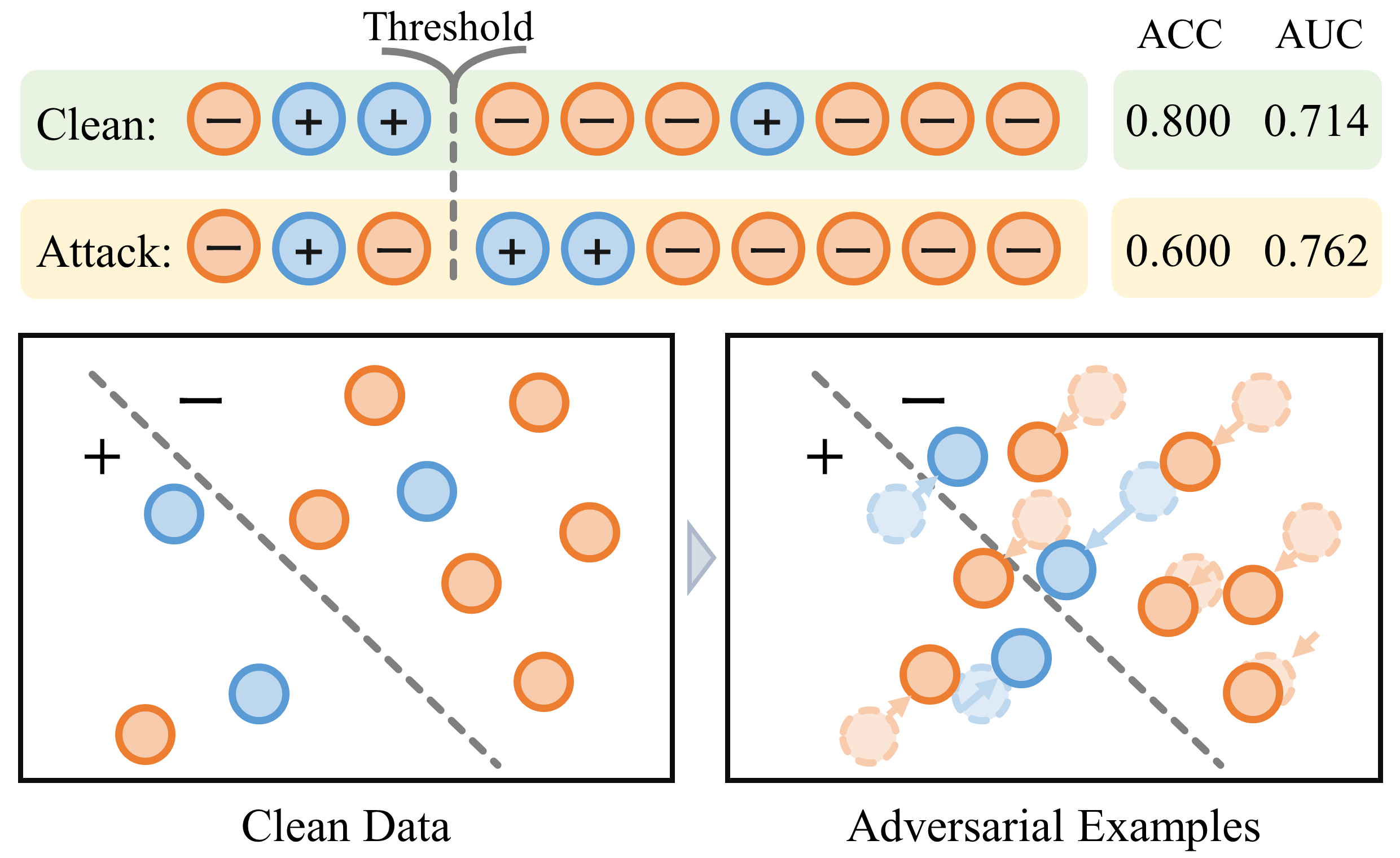
Figure 1: Diagram of ACC and AUC change when the model is attacked. The upper rectangular boxes represent the score rank before and after the attack occurs; The lower plots represent the change of score in the embedding space when the model is attacked.

Deep learning has recently achieved significant progress on various machine learning tasks, such as computer vision (Voulodimos et al., 2018) and natural language processing (Strubell et al., 2019; Sorin et al., 2020). However, recent work shows that deep learning models are vulnerable to adversarial attack (Szegedy et al., 2014; Biggio et al., 2013). For example, images with human imperceptible perturbations (i.e., adversarial examples) can easily fool even the well-trained models. The existence of adversarial examples has raised big security threats to deep neural networks, which impels extensive efforts to improve the adversarial robustness (Madry et al., 2018; Zhang et al., 2019b). For example, one can resist the adversarial examples by means of adversarial training (AT). Specifically, AT could be formulated as a min-max problem, where the inner maximization problem is employed to generate adversarial examples, and the outer minimization problem is used to learn the model under the adversarial noise. In this way, AT could be easily applied to most of the modern architectures in deep learning, making it one of the most effective measures against adversarial attack.

The prior art of adversarial training methods focuses on balanced benchmark datasets. On top of this, the learning objective is to increase the overall accuracy. However, real-world datasets usually exhibit a long-tail distribution that the proportion of the majority classes examples significantly dominates the others. For such long-tail problems, accuracy (ACC) is considered to be a less appropriate performance metric than another metric named AUC (Area Under the ROC Curve). Specifically, AUC is the probability of observing a positive instance with a higher score than a negative one. It is well-known to be insensitive to class distributions and costs (Fawcett, 2006; Hand & Till, 2001). Comparing AUC with ACC, we then ask:

Can we improve the adversarial robustness of AUC by employing the traditional ACC-based methods?

Unfortunately, the answer might be negative. As shown in Fig.1, the adversarial examples generated by minimizing ACC (ACC drops from 0.8 to 0.6), may fail to attack AUC (AUC here increases from 0.714 to 0.762). In this sense, the model trained on such adversarial examples cannot improve the adversarial robustness of AUC. Therefore, more attention should be paid to AUC when studying the adversarial robustness against long-tail problems.

Inspired by this fact, we present a very early trial to study adversarial training in AUC optimization with an end-to-end framework.

Existing AT methods can be easily implemented in an end-to-end manner since the inner maximization problem for generating the adversarial examples can be solved instance-wisely. However, this is not the case for AUC optimization. Specifically, in the expression of AUC, every positive instance is coupled with all the negative instances and vice versa. For a binary class classification problem, this means that we need to spend $O(n^{-}\cdot T)$ time for generating the adversarial example of a positive instance and $O(n^{+}\cdot T)$ for a negative one, where $n^{+},n^{-}$ are the number of positive and negative instances, and $T$ is complexity for calculating the gradient for a single positive-negative instance pair. In this sense, we can hardly implement such a naive training method on top of even the simplest deep learning framework.

To solve the challenge, this paper proposes an end-to-end adversarial AUC optimization framework with a convergence guarantee. Specifically, our contribution is as follows:

First, based on a reformulation technique and a concavity regularizer, we show that the original problem is equivalent to a min-max problem where the objective function can be expressed in an instance-wise manner.

Second, we propose an AT algorithm to optimize the min-max problem, where we alternately invoke a projected-gradient-descent-like protocol to generate the adversarial examples, and a stochastic gradient descent-ascent protocol to train the model parameters. Meanwhile, we also present a convergence analysis to show the correctness of our algorithm. The proof here is non-trivial since we have to simultaneously estimate the gradient of the min player and the max player.

Finally, we conduct a series of empirical analyses of our proposed algorithm on long-tail datasets. The results demonstrate the effectiveness of our proposed method.

2 Related Work

2.1 AUC Optimization

As a motivating study, (Cortes & Mohri, 2003) investigates the inconsistency between AUC maximization and error rate minimization, which shows the necessity to study direct AUC optimization methods. After that, a series of algorithms are designed for off-line AUC optimization (Herschtal & Raskutti, 2004; Joachims, 2005). To extend the scalability of AUC optimization, researchers start to explore the online and stochastic optimization extensions of the AUC maximization problem. (Zhao et al., 2011) makes the first attempt for this direction based on the reservoir sampling technique. (Gao et al., 2013) proposes a one-pass AUC optimization algorithm based on the squared surrogate loss. After that, (Ying et al., 2016) reformulates the minimization problem of the pairwise square loss into an equivalent stochastic saddle point problem, where the objective function could be expressed in an instance-wise manner. On top of the reformulation framework, (Natole et al., 2018) proposes an accelerated version with a faster convergence rate and (Liu et al., 2019) explores its extension in deep neural networks. Meanwhile, many researchers provide theoretical guarantees for AUC optimization algorithms from different aspects, such as generalization analysis (Agarwal et al., 2005; Clémençon et al., 2008; Usunier et al., 2005) and consistency analysis (Agarwal, 2014; Gao & Zhou, 2015). Beyond the optimization algorithms and theoretical supports for AUC, in practice, AUC optimization demonstrates its effectiveness in various class-imbalanced tasks, such as disease prediction (Westcott et al., 2019; Gola et al., 2020; Ren et al., 2018), rare event detection (Feizi, 2020; Robles et al., 2020) and etc.

Compared with the existing study, we present a very early trial for the adversarial training problem.

2.2 Adversarial Training

For a long time, machine learning models have proved vulnerable to adversarial examples (Biggio et al., 2013; Szegedy et al., 2014; Goodfellow et al., 2014). Numerous defenses have been proposed to address the security concern raised by the issue (Athalye & Carlini, 2018; Athalye et al., 2018). Among such studies, adversarial training is one of the most popular methods (Kurakin et al., 2017; Madry et al., 2018; Zhang et al., 2019b). The majority of studies in this direction follows the min-max formulation proposed in (Madry et al., 2018), which so far has been improved in various way (Shafahi et al., 2020; Cai et al., 2018; Tramèr et al., 2017; Pang et al., 2019; Wang et al., 2019b; Zhang et al., 2020; Maini et al., 2020; Tramèr & Boneh, 2019). Furthermore, due to the heavy computational burden of AT, accelerating the training procedure of AT becomes increasingly urgent. Recently, there has been a new wave to explore the acceleration of AT, which includes reusing the computations (Shafahi et al., 2019; Zhang et al., 2019a), adaptive adversarial steps (Wang et al., 2019a) and one-step training (Wong et al., 2019). Besides the practical improvements, there are also some recent advances in theoretical investigations from the perspective of optimization (Wang et al., 2019a; Bai et al., 2022), generalization (Xing et al., 2021; Tu et al., 2019), and consistency (Bao et al., 2020).

In this paper, we will present an AT algorithm on top of the AUC optimization. As shown in the introduction, the complicated expression of AUC brings new elements into our model formulation and theoretical analysis.

3 Preliminaries

In this section, we briefly introduce the AUC optimization problem and the adversarial training framework.

3.1 AUC Optimization Problem

Let $X$ be the feature set. Based on (Hanley & McNeil, 1982), AUC of a scoring function $h_{\theta}:X\rightarrow[0,1]$ is equivalent to the probability that a positive instance is predicted with a higher score compared to a negative instance:

$$\mathsf{AUC}(h_{\theta})=\mathrm{Pr}\left(h_{\theta}(\bm{x}^{+})\geq h_{\theta}(\bm{x}^{-})|y^{+}=1,y^{-}=0\right),$$

where $(\bm{x}^{+},y^{+})$ and $(\bm{x}^{-},y^{-})$ represent positive and negative examples, respectively, and $\theta$ is the model parameters. By employing a differentiable loss $\ell$ as the surrogate loss, the unbiased estimation of $\mathsf{AUC}(h_{\theta})$ could be expressed as:

$$\hat{\mathsf{AUC}}(h_{\theta})=1-\sum_{i=1}^{n^{+}}\sum_{j=1}^{n^{-}}\frac{\ell\left(h_{\theta}(\bm{x}^{+})-h_{\theta}(\bm{x}^{-})\right)}{n^{+}n^{-}}.$$

where $n^{+}$ and $n^{-}$ denote the number of positive and negative examples, respectively. Then AUC maximization problem is equivalent to the following minimization problem:

$${\color[rgb]{0.45703125,0.6171875,0.22265625}\textbf{(OP0)}}~{}~{}\min\limits_{\bm{\theta}}\mathcal{L}(\bm{\theta},\bm{x},y):=\sum_{i=1}^{n^{+}}\sum_{j=1}^{n^{-}}\frac{\ell\left(h_{\theta}(\bm{x}^{+})-h_{\theta}(\bm{x}^{-})\right)}{n^{+}n^{-}}.$$

Table 1: Notations and their description

Notations	Description
$n$	Number of total examples
$n^{+}$, $n^{-}$	Number of positive (negative) examples
$p$	Proportion of positive examples
$\bm{x}^{0}$	Clean Examples
$\bm{x}^{k}$	Adversarial examples generated in step $k$
$y$	The label of example
$\bm{\delta}$	Perturbation on samples
$\mathcal{X}_{i}$	$\mathcal{X}_{i}=\{\bm{x}|\left\|\bm{x}-\bm{x}_{i}^{0}\right\|_{\infty}\leq\epsilon\}$
$\bm{\theta}$	Parameters of model
$a,b,\alpha$	Learnable parameters of loss function
$\bm{w}$	$\bm{w}=(\bm{\theta},a,b)$
$f(\bm{w},\alpha,\bm{x})$	The surrogate objective function
$L(\bm{w},\alpha)$	$\frac{1}{n}\sum_{i=1}^{n}f(\bm{w},\alpha,\bm{x}_{i}^{*})$
$\Phi(\bm{w})$	$\Phi(\bm{w})=\max_{\alpha}L(\bm{w},\alpha)$
$\mathcal{B}$	The mini-batch
$M$	The batch size
$L$	$\max\{L_{ww},L_{wx},L_{\alpha\alpha},L_{\alpha{x}},L_{{x}w},L_{x\alpha}\}$
$T$	The total of training epochs
$\hat{g}(\alpha),\hat{g}(\bm{w})$	Stochastic gradient
$g(\alpha),g(\bm{w})$	Stochastic gradient

3.2 Adversarial Training Framework

Adversarial training is one of the most effective defensive strategies against adversarial examples (Goodfellow et al., 2015; Madry et al., 2018), the key idea of which is to directly optimize the model performance based on the perturbed examples. Generally speaking, the adversarial training framework can be formalized as

$$\min\limits_{\bm{\theta}}\frac{1}{n}\sum_{i=1}^{n}\max\limits_{\left\|\bm{\delta}_{i}\right\|_{\infty}\leq\epsilon}\ell(h_{\theta}(\bm{x}_{i}^{0}+\bm{\delta}_{i}),y_{i}).$$ (1)

Here $\bm{\delta}_{i}$ is the perturbation on clean feature vector $\bm{x}_{i}^{0}$, and $\bm{x}_{i}=\bm{x}_{i}^{0}+\bm{\delta}_{i}$ is the resulting adversarial example for the instance $(\bm{x}_{i}^{0},y_{i}),i=1,2,\cdots,n$. The inner maximization problem generates such adversarial examples by trying to hurt the model performance (by maximizing the loss $\ell(h_{\theta}(\bm{x}_{i}^{0}+\bm{\delta}_{i}),y)$). The constraint $\left\|\bm{\delta}_{i}\right\|_{\infty}\leq\epsilon$ makes sure that the adversarial perturbation is small enough to be imperceptible. In this sense, the adversarial example lives in $\mathcal{X}_{i}=\left\{\bm{x}|\left\|\bm{x}-\bm{x}^{0}_{i}\right\|_{\infty}\leq\epsilon\right\}$. Finally, the outer minimization problem is to find a robust model that can resist the adversarial perturbation.

For the inner maximization problem, K-PGD (Madry et al., 2018) is a widely used attack method that perturbs the clean examples $\bm{x}^{0}$ iteratively with a total of K steps. At the end of each iteration, the example will be projected to the $\epsilon$-ball of $\bm{x}^{0}$. Specifically, the adversarial examples generated in $k+1$ step are as follows:

$$\bm{x}^{k+1}=\mathrm{Proj}\big{\{}\bm{x}^{k}+\beta\cdot\operatorname{sign}(\nabla_{\bm{x}}\ell(h_{\theta}(\bm{x}^{k}),y^{k}))\big{\}},$$ (2)

where $\mathrm{Proj}$ is the projection function, and $\beta$ is the step size. For the outer minimization problem, gradient descent is usually used to solve it. A more detailed introduction of adversarial attack methods is shown in the Appendix B.

4 Methodology

Before entering into the methodology, we summarize some useful notations in Tab.1 to make our argument easier to follow.

4.1 Reformulation of Optimization Problem

A naive idea to perform AUC adversarial training is to directly combine (OP0)  with the standard AT framework (Madry et al., 2018), resulting in the following problem:

$$\min\limits_{\bm{\theta}}\max\limits_{\bm{\delta}_{1},\bm{\delta}_{2},\cdots,\bm{\delta}_{n}}\sum_{i=1}^{n^{+}}\sum_{j=1}^{n^{-}}\frac{\ell(h_{\theta}(\bm{x}_{i}^{+}+\bm{\delta}_{i})-h_{\theta}(\bm{x}_{j}^{-}+\bm{\delta}_{j}))}{n^{+}n^{-}},$$

According to the definition of AUC optimization objective function $\mathcal{L}$ in (OP0) , we know that each pair of positive examples is inter-dependent with all negative examples, and vice versa for the negative examples. Thus, the inner maximization problem for $\bm{\delta}_{1},\bm{\delta}_{2},\cdots,\bm{\delta}_{n}$ cannot be decoupled into a series of instance-wise maximization problems. In other words, the following inequality holds in general:

$$\min\limits_{\bm{\theta}}\max\limits_{\bm{\delta}_{1},\bm{\delta}_{2},\cdots,\bm{\delta}_{n}}\sum_{i=1}^{n^{+}}\sum_{j=1}^{n^{-}}\frac{\ell(h_{\theta}(\bm{x}_{i}^{+}+\bm{\delta}_{i})-h_{\theta}(\bm{x}_{j}^{-}+\bm{\delta}_{j}))}{n^{+}n^{-}}$$

$$\neq$$

$$\min\limits_{\bm{\theta}}\sum_{i=1}^{n^{+}}\sum_{j=1}^{n^{-}}\max\limits_{\bm{\delta}_{i},\bm{\delta}_{j}}\frac{\ell(h_{\theta}(\bm{x}_{i}^{+}+\bm{\delta}_{i})-h_{\theta}(\bm{x}_{j}^{-}+\bm{\delta}_{j}))}{n^{+}n^{-}}.$$

In this sense, the generation of adversarial examples cannot be carried out in a mini-batch fashion. Instead, one update $\bm{\delta}$ requires a full scan of $O(n^{+}n^{-})$. This brings a heavy computational burden towards its application. Therefore, we need to reformulate the optimization problem.

Fortunately, if we adopt the square loss $\ell(t)=(1-t)^{2}$ as the surrogate loss function, then (Ying et al., 2016; Liu et al., 2019) proved that (OP0)  could be converted in a min-max problem, as shown in the following proposition:

Proposition 1.

The empirical risk of AUC in (OP0)  is equivalent to

$$\mathcal{L}(\bm{\theta},\bm{x},y)=\min\limits_{a,b}\max\limits_{\alpha}\frac{1}{n}\sum^{n}_{i=1}g(\bm{\theta},a,b,\alpha,(\bm{x}_{i},y_{i})),$$ (3)

where

$$g (\bm{\theta},a,b,\alpha,(\bm{x}_{i},y_{i}))$$ (4)

$$= (1-p)(h_{\theta}(\bm{x}_{i})-a)^{2}\mathbb{I}_{[y_{i}=1]}+p(h_{\theta}(\bm{x}_{i})-b)^{2}\mathbb{I}_{[y_{i}=0]}$$

$$+2(1+\alpha)\left(ph_{\theta}(\bm{x}_{i})\mathbb{I}_{[y_{i}=0]}-(1-p)h_{\theta}(\bm{x}_{i})\mathbb{I}_{[y_{i}=1]}\right)$$

$$-p(1-p)\alpha^{2}.$$

where $a,b,\alpha\in\mathbb{R}$ are learnable parameters, and $p=\mathrm{Pr}(y=1)$.

Remark 1.

According to (Ying et al., 2016), $a,b,\alpha$ has the following closed-form solution: $a=\hat{\mathbb{E}}[h_{\theta}(\bm{x})|y=1]$, $b=\hat{\mathbb{E}}[h_{\theta}(\bm{x})|y=0]$ and $\alpha=\hat{\mathbb{E}}[h_{\theta}(\bm{x})|y=0]-\hat{\mathbb{E}}[h_{\theta}(\bm{x})|y=1]$, where $\hat{\mathbb{E}}$ is a shorthand for sample mean. If the score $h_{\theta}$ is normalized to the set $[0,1]$, we can restrict $a,b$ and $\alpha$ to the following bounded domains:

$$\Omega_{a,b}=\left\{a,b\in\mathbb{R}|0\leq a,b\leq 1\right\},\Omega_{\alpha}=\left\{\alpha\in\mathbb{R}||\alpha|\leq 1\right\}.$$

And we can easily verify that $g$ is $\mu$-strongly concave w.r.t. $\alpha$ in $\Omega_{\alpha}$, i.e., for any $\alpha_{1},\alpha_{2}\in\Omega_{\alpha}$, it holds that

$$g(\bm{\theta}, a,b,\alpha_{1},(\bm{x},y))\leq g(\bm{\theta},a,b,\alpha_{2},(\bm{x},y))+$$

$$\langle\nabla_{\alpha}g(\bm{\theta},a,b,\alpha_{2},(\bm{x},y)),\alpha_{1}-\alpha_{2}\rangle-\frac{\mu}{2}\left\|\alpha_{1}-\alpha_{2}\right\|_{2}^{2}.$$

And we can also verified that $g$ is locally strongly convex in $\Omega_{a,b}$ w.r.t. $a$ and $b$.

Hence, if we in turn construct an AT problem based on Prop.1, we can obtain the following optimization problem with ease:

$$\min\limits_{\bm{\theta}}\max\limits_{\bm{\delta}}\min\limits_{a,b\in\Omega_{a,b}}\max_{\alpha\in\Omega_{\alpha}}\frac{1}{n}\sum^{n}_{i=1}g(\bm{\theta},a,b,\alpha,(\bm{x}_{i}+\bm{\delta}_{i},y_{i})).$$

The good news here is that in the new loss function $g$, positive samples and negative samples are independent of each other. However, the bad news is that the min-max-min-max problem is still hardly tractable. Through a careful investigation, if we can swap the order of $\min_{a,b}$ and $\max_{\bm{\delta}}$, we can then obtain a min-max problem which can be solved in an end-to-end fashion. To realize the idea, we could resort to the von Neumann’s Minimax theorem (Neumann, 1928; Sion, 1958):

Theorem 1.

Let $X\subset\mathbb{R}^{n}$ and $Y\subset\mathbb{R}^{m}$ be compact convex sets. If $f:X\times Y\rightarrow\mathbb{R}$ is a continuous function that is concave-convex, i.e.

$$f(\cdot,\bm{y}):X\rightarrow\mathbb{R}\text{ is concave for fixed $\bm{y}$,}$$

$$f(\bm{x},\cdot):Y\rightarrow\mathbb{R}\text{ is convex for fixed $\bm{x}$.}$$

Then we have that $\max\limits_{\bm{x}\in X}\min\limits_{\bm{y}\in Y}f(\bm{x},\bm{y})=\min\limits_{\bm{y}\in Y}\max\limits_{\bm{x}\in X}f(\bm{x},\bm{y})$.

Moreover, we resort to the definition of weak-concavity (Böhm & Wright, 2021; Liu et al., 2021):

Definition 1.

$f(\bm{x}):\mathbb{R}^{d}\rightarrow\mathbb{R}$ is said to be a $\gamma$-weakly concave ($\gamma>0$) function w.r.t. $\bm{x}$, if

$$f(\bm{x})-\frac{\gamma}{2}||\bm{x}||_{2}^{2}$$

is a concave function w.r.t. $\bm{x}$.

In the following proposition, we find a surrogate objective function $f(\bm{w},\alpha,\bm{x}_{i}+\bm{\delta}_{i})$ such that the resulting optimization problem could be reformulated as a min-max problem:

Proposition 2.

Define:

$$r(a,b,\bm{x})=\max_{\alpha}\frac{1}{n}\sum^{n}_{i=1}g(\bm{\theta},a,b,\alpha,(\bm{x}_{i}+\bm{\delta}_{i},y_{i})),$$

$$f(\bm{w},\alpha,\bm{x}_{i}+\bm{\delta}_{i})=g(\bm{\theta},a,b,\alpha,(\bm{x}_{i}+\bm{\delta}_{i},y_{i}))$$

$$~{}~{}~{}~{}~{}~{}~{}~{}~{}~{}~{}~{}~{}~{}~{}~{}~{}~{}~{}~{}~{}~{}~{}~{}~{}~{}~{}~{}~{}~{}~{}~{}-\gamma\left\|\bm{x}_{i}+\bm{\delta}_{i}\right\|^{2}_{2}$$

If $r(a,b,\bm{x})$ is $\gamma_{*}$-weakly concave w.r.t. $\bm{\delta}_{1},\bm{\delta}_{2},\cdots,\bm{\delta}_{n}$, then for all $\gamma>\gamma_{\star}$, we have the following problem:

$$\small\min\limits_{\bm{\theta}}\max\limits_{\bm{\delta}}\min\limits_{a,b\in\Omega_{a,b}}\max_{\alpha\in\Omega_{\alpha}}\frac{1}{n}\sum^{n}_{i=1}f(\bm{w},\alpha,(\bm{x}_{i}+\bm{\delta}_{i},y_{i}))$$

is equivalent to:

(OP) $$\min\limits_{\bm{w}}\max\limits_{\alpha}\max\limits_{\bm{\delta}}\frac{1}{n}\sum^{n}_{i=1}\left[f(\bm{w},\alpha,\bm{x}_{i}+\bm{\delta}_{i})\right]$$

$$=\min\limits_{\bm{w}}\max\limits_{\alpha}\frac{1}{n}\sum^{n}_{i=1}\max\limits_{\bm{\delta}_{i}}\left[f(\bm{w},\alpha,\bm{x}_{i}+\bm{\delta}_{i})\right],$$

where $\bm{w}=(\bm{\theta},a,b)$. Moreover, $f(\bm{w},\alpha,\bm{x}_{i}+\bm{\delta}_{i})$ is strongly concave w.r.t. $\bm{\delta}_{i}$.

Remark 2.

According to (Böhm & Wright, 2021; Liu et al., 2021), if $\max_{\alpha}\frac{1}{n}\sum^{n}_{i=1}\left[f(\bm{w},\alpha,\bm{x}_{i}+\bm{\delta}_{i})\right]$ is smooth and $L$ gradient Lipschitz, then it is also $L$-weakly concave. Hence, the weakly concavity assumption is much weaker than the strongly-concave assumption (Wang et al., 2019a).

In this sense, we could turn to optimize (OP) in the next subsection.

4.2 Training Strategy

In this subsection, we continue to propose an adversarial AUC optimization framework to solve (OP). Specifically, we design solutions for the inner maximization problem and the outer min-max problem, respectively.

Inner Maximization Problem: Adversarial Attack. In this paper, we choose K-PGD (Madry et al., 2018) to generate adversarial examples. To better control the quality of adversarial examples, we introduce the First-Order Stationary Condition (FOSC) (Wang et al., 2019a) about the inner maximization problem, which is as follows:

$$c(\bm{x}^{k})=\max\limits_{\bm{x}\in\mathcal{X}}\langle\bm{x}-\bm{x}^{k},\nabla_{\bm{x}}f(\bm{w},\alpha,\bm{x}^{k})\rangle$$ (5)

When $c(\bm{x}^{k})=0$, the optimization problem reaches the convergence state. Specifically, such a condition can be achieved when a) $\nabla_{\bm{x}}f(\bm{w},\alpha,\bm{x}^{k})=0$, or b) $\bm{x}^{k}-\bm{x}^{0}=\epsilon\cdot\operatorname{sign}\left(\nabla_{\bm{x}}f(\bm{w},\alpha,\bm{x}^{k})\right)$. Here a) implies $\bm{x}^{k}$ is a stationary point in the inner maximization problem, b) shows that local maximum point of $f(\bm{w},\alpha,\bm{x}^{k})$ reaches the boundary of $\mathcal{X}$. The proof process is shown in Lem.1.

Algorithm 1 Adversarial Training for AUC Optimization

  Input:Neural network $h_{\theta}$; initial parameters $\bm{w}_{0}=\{\bm{\theta}^{0},a^{0},b^{0}\}$ and $\alpha^{0}$; step size $\eta_{w}$, $\eta_{\alpha}$; mini-batch $\mathcal{B}$ and its size $M$; max FOSC value $c_{max}$; training epochs $T$; control epoch $T^{\prime}$; PGD step $K$; PGD step size $\beta$; maximum perturbation boundary $\epsilon$.

  for $t=0$ to $T$ do

     $c_{t}=\max(0,c_{max}-t\cdot c_{max}/{T^{\prime}})$

     for Each batch $\bm{x}_{\mathcal{B}}^{0}$ do

        $M_{c}=\mathbbm{1}_{\mathcal{B}}$; $k=0$

        while $\sum M_{c}>0\ \ \&\ \ k<K$ do

           $\bm{x}^{k+1}_{\mathcal{B}}=\bm{x}^{k}_{\mathcal{B}}+M_{c}\cdot\beta\cdot sign(\nabla_{\bm{x}}\ell(h_{\theta}(\bm{x}^{k}_{\mathcal{B}}),y))$

           $\bm{x}^{k+1}_{\mathcal{B}}=clip(\bm{x}^{k+1}_{\mathcal{B}},\bm{x}^{k+1}_{\mathcal{B}}-\epsilon,\bm{x}^{k+1}_{\mathcal{B}}+\epsilon)$

           $M_{c}=\mathbbm{1}_{\mathcal{B}}(c(x_{1\dots M}^{k+1})\leq c_{t})$

           $k=k+1$

        end while

        $\alpha^{t+1}=\alpha^{t}+\eta_{\alpha}\hat{g}(\alpha)$

        $\bm{w}^{t+1}=\bm{w}^{t}-\eta_{w}\hat{g}(\bm{w})$   # $\hat{g}$: stochastic gradient

     end for

  end for

  return $\bm{w}^{T},\alpha^{T}$

Outer min-max Problem. For the outer min-max problem, we apply Stochastic Gradient Descent Ascent (SGDA) to solve the problem. At each iteration, SGDA performs stochastic gradient descent over the parameter $\bm{w}$ with the stepsize $\eta_{w}$, and stochastic gradient ascent over the parameter $\alpha$ with the stepsize $\eta_{\alpha}$.

The total training strategy is presented in Alg.1. This is an extension of the algorithm proposed in (Wang et al., 2019a), where the outer level minimization problem now becomes a min-max problem. The value of FOSC can imply the adversarial strength of adversarial examples, whereas a small FOSC value implies a high adversarial strength. Due to this fact, through the FOSC value of current epoch $c_{t}$, we can dynamically control the strength of adversarial examples. Specifically, in the initial stage of training, the value of $c_{t}$ is large, which means the generated adversarial examples are not so hard. In the later stage of training, the value of $c_{t}$ is 0, which allows model to be trained on much stronger adversarial examples. Consequently, such an algorithm will allow the model to learn from in a progressive manner. Here, we use $M_{c}$ to mask the examples that satisfy the condition in the Line 9 in Alg.1. By doing so, we can ensure that the FOSC values of the adversarial examples generated by Alg. 1 are all less than $c_{max}$. When the adversarial examples are obtained, we calculate the stochastic gradient of the parameters $\bm{w}$ and $\alpha$. Then we perform stochastic gradient descent-ascent on $\bm{w}$ and $\alpha$ respectively.

4.3 Convergence Analysis

Next, we provide a convergence analysis of our proposed adversarial AUC optimization framework.

We first give the definition and description of some notations. In detail, let $\bm{x}^{*}_{i}(\bm{w},\alpha)=\arg\max_{\bm{x}_{i}\in\mathcal{X}_{i}}f(\bm{w},\alpha,\bm{x}_{i})$ where $\mathcal{X}_{i}=\left\{\bm{x}|\left\|\bm{x}-\bm{x}_{i}^{0}\right\|_{\infty}\leq\epsilon\right\}$. And

$$L(\bm{w},\alpha) =\frac{1}{n}\sum_{i=1}^{n}\max\limits_{\bm{x}_{i}\in\mathcal{X}_{i}}f(\bm{w},\alpha,\bm{x}_{i})=\frac{1}{n}\sum_{i=1}^{n}f(\bm{w},\alpha,\bm{x}_{i}^{*}).$$

Then $\hat{\bm{x}}_{i}(\bm{w},\alpha)$ is a $\delta$-approximate solution to $\bm{x}_{i}^{*}(\bm{w},\alpha)$, if it satisfies that

$$\max\limits_{\bm{x}\in\mathcal{X}_{i}}\langle\bm{x}-\hat{\bm{x}}_{i}(\bm{w},\alpha),\nabla_{\bm{x}}f(\bm{w},\alpha,\hat{\bm{x}}_{i}(\bm{w},\alpha))\rangle\leq\delta.$$ (6)

Furthermore, let $\nabla L(\alpha)$ denote the gradient of $L(\bm{w},\alpha)$ w.t.r. $\alpha$. And let $g(\alpha)=\frac{1}{M}\sum_{i\in\mathcal{B}}\nabla_{\alpha}f(\bm{w},\alpha,\bm{x}_{i}^{*})$ be the stochastic gradient of $L(\bm{w},\alpha)$ w.r.t. $\alpha$, where $\mathcal{B}$ is mini-batch and $M=|\mathcal{B}|$. Meanwhile, let $\nabla_{\alpha}f(\bm{w},\alpha,\hat{\bm{x}}(\bm{w},\alpha))$ be the gradient of $f(\bm{w},\alpha,\hat{\bm{x}}(\bm{w},\alpha))$ w.r.t. $\alpha$, and let $\hat{g}(\alpha)=\frac{1}{M}\sum_{i\in\mathcal{B}}f(\bm{w},\alpha,\hat{\bm{x}}_{i})$ be the approximate stochastic gradient of $L(\bm{w},\alpha)$ w.r.t. $\alpha$. And for $\bm{w}$, we have the same definition as $\alpha$. In addition, let

$$\Phi(\bm{w})=\max\limits_{\alpha}L(\bm{w},\alpha),~{}~{}~{}\nabla\Phi(\bm{w})=\nabla_{\bm{w}}L(\bm{w},\alpha^{*}(\bm{w})).$$

Then, before giving the convergence analysis, we list some assumptions needed to the analysis.

Assumption 1.

The function $f(\bm{w},\alpha,\bm{x})$ satisfies the gradient Lipschitz conditions as follows:

$$\sup\limits_{\alpha,\bm{x}}\left\|\nabla_{\bm{w}}f(\bm{w},\alpha,\bm{x})-\nabla_{\bm{w}}f(\bm{w}^{\prime},\alpha,\bm{x})\right\|_{2}\leq L_{ww}\left\|\bm{w}-\bm{w}^{\prime}\right\|_{2}$$

$$\sup\limits_{\alpha,\bm{w}}\left\|\nabla_{\bm{w}}f(\bm{w},\alpha,\bm{x})-\nabla_{\bm{w}}f(\bm{w},\alpha,\bm{x}^{\prime})\right\|_{2}\leq L_{wx}\left\|\bm{x}-\bm{x}^{\prime}\right\|_{2}$$

$$\sup\limits_{\alpha,\bm{x}}\left\|\nabla_{\bm{x}}f(\bm{w},\alpha,\bm{x})-\nabla_{\bm{x}}f(\bm{w}^{\prime},\alpha,\bm{x})\right\|_{2}\leq L_{xw}\left\|\bm{w}-\bm{w}^{\prime}\right\|_{2}$$

$$\sup\limits_{\bm{w},\bm{x}}\left\|\nabla_{\alpha}f(\bm{w},\alpha,\bm{x})-\nabla_{\alpha}f(\bm{w},\alpha^{\prime},\bm{x})\right\|_{2}\leq L_{\alpha\alpha}\left\|\alpha-\alpha^{\prime}\right\|_{2}$$

$$\sup\limits_{\bm{w},\alpha}\left\|\nabla_{\alpha}f(\bm{w},\alpha,\bm{x})-\nabla_{\alpha}f(\bm{w},\alpha,\bm{x}^{\prime})\right\|_{2}\leq L_{\alpha x}\left\|\bm{x}-\bm{x}^{\prime}\right\|_{2}$$

$$\sup\limits_{\bm{w},\bm{x}}\left\|\nabla_{\bm{x}}f(\bm{w},\alpha,\bm{x})-\nabla_{\bm{x}}f(\bm{w},\alpha^{\prime},\bm{x})\right\|_{2}\leq L_{x\alpha}\left\|\alpha-\alpha^{\prime}\right\|_{2}$$

where $L_{\alpha\alpha},L_{\alpha x},L_{x\alpha},L_{ww},L_{wx},L_{xw}$ are positive constants.

Remark 3.

The first three gradient Lipschitz conditions in Asm.1 are made in (Sinha et al., 2018), and the last three gradient Lipschitz conditions are made in (Liu et al., 2019). Meanwhile, for the overparameterized deep neural network, the loss function is semi-smooth (Allen-Zhu et al., 2019; Du et al., 2019), which helps to justify Asm.1.

Assumption 2.

$\left\|\nabla_{\bm{w}}f(\bm{w},a,\bm{x})\right\|_{2}$ is upper bounded by $l_{w}$.

Remark 4.

Asm.2 is widely used in minimax optimization problems (Sinha et al., 2018).

Assumption 3.

$f(\bm{w},\alpha,\bm{x})$ is locally $\mu$-strongly concave in $\mathcal{X}_{i}$ for all $i\in[n]$, i.e. for any $\bm{x}_{1},\bm{x}_{2}\in\mathcal{X}_{i}$, it holds that

$$f(\bm{w}, \alpha,\bm{x}_{1})\leq f(\bm{w},\alpha,\bm{x}_{2})+$$

$$\langle\nabla_{\bm{x}}f(\bm{w},\alpha,\bm{x}_{2}),\bm{x}_{1}-\bm{x}_{2}\rangle-\frac{\mu}{2}\left\|\bm{x}_{1}-\bm{x}_{2}\right\|_{2}^{2}$$

Remark 5.

The strongly concave assumption is equivalent to weakly concave assumption of $r$, which is much easier to be achieved.

Assumption 4.

The stochastic gradient $g(\alpha)$ satisfies

$$\mathbb{E}[g(\alpha)-\nabla L(\alpha)]=0, \mathbb{E}\left[\left\|g(\alpha)-\nabla L(\alpha)\right\|^{2}_{2}\right]\leq\sigma^{2}$$

$$\mathbb{E}[g(\bm{w})\!-\!\nabla L(\bm{w})]=0, \mathbb{E}\left[\left\|g(\bm{w})-\nabla L(\bm{w})\right\|^{2}_{2}\right]\leq\sigma^{2}$$

Remark 6.

Asm.4 is a common assumption used to analyze the optimization algorithm based on stochastic gradient (Lin et al., 2020; Liu et al., 2019).

Theorem 2.

Under the above assumptions and let the stepsizes be chosen as $\eta_{w}=\Theta\left(1/\kappa^{2}L\right)$, $\eta_{\alpha}=\Theta(1/L)$ and $\kappa\leq\frac{7}{6}$, then we have the following inequality:

$$\frac{1}{T+1} \left(\sum_{t=0}^{T}\mathbb{E}\left[\left\|\nabla\Phi(\bm{w}_{t})\right\|_{2}^{2}\right]\right)$$

$$\leq\frac{360\kappa^{2}L\Delta_{\Phi}+13\kappa L^{2}D^{2}}{T+1}+\frac{26\kappa\sigma^{2}}{M}+h_{\delta}+h_{\Delta}$$

where $h_{\delta}=\frac{1024}{253}\left(\frac{3\kappa L\delta}{1024}+6\kappa^{4}L\delta+\frac{L\delta}{8}+L^{2}\sqrt{\frac{\delta}{\mu}}\right)$ and $h_{\Delta}=\frac{384\kappa^{4}L^{2}\Delta}{253}$ and $\Delta_{\Phi}=\Phi(\bm{w}^{0})-\min_{\bm{w}}\Phi(\bm{w})$, $D=|\Omega_{\alpha}|$, $L$ denotes the maximum in Lipschitz constant, and the condition number $\kappa=L/\mu$.

Remark 7.

On the right side of the inequality, the first term is an $O(1/T)$ magnitude, the last three terms behave as the residuals. The second term $\frac{26\kappa\sigma^{2}}{M}$ is related to the batch size $M$. As $M$ increases, its value gradually tends to 0. The third term $h_{\delta}$ is due to the use of an approximate solution $\hat{\bm{x}}$ to the inner maximization problem instead of the optimal solution $\bm{x}^{*}$, and the fourth term $h_{\Delta}$ is due to $\mathcal{X}$ being a bounded set. Since all of the residuals are small, we can find an $\epsilon$-stationary point within a finite number of epochs.

5 Experiments

In this section, we evaluate the performance of our AdAUC algorithms in three long-tail datasets.

Table 2: Test AUC and robustness of models trained with various methods. We mark the best performance with Bold and the second best performance with underscore.

Dataset	Method	Training	Evaluated Against
			Clean	FSGM	PGD-5	PGD-10	PGD-20	C$\&$W	AA
CIFAR-10-LT	CE	NT	0.7264	0.4038	0.0753	0.0206	0.0044	0.0009	0.0082
		AT1	0.6659	0.5487	0.3335	0.2743	0.2344	0.2330	0.2678
		AT2	0.6833	0.6296	0.4870	0.4417	0.4319	0.4310	0.4384
	AdAUC	NT	0.7885	0.6606	0.2671	0.1892	0.0064	0.0573	0.0740
		AT1	0.7347	0.6646	0.5236	0.4625	0.4224	0.3927	0.4362
		AT2	0.7528	0.6952	0.5591	0.5309	0.5283	0.5283	0.5291
CIFAR-100-LT	CE	NT	0.6382	0.1207	0.0271	0.0159	0.0110	0.0102	0.0123
		AT1	0.6193	0.5183	0.3195	0.2750	0.2668	0.2630	0.2703
		AT2	0.6198	0.5192	0.3183	0.2767	0.2681	0.2647	0.2712
	AdAUC	NT	0.6462	0.5161	0.3046	0.1818	0.1214	0.0035	0.1313
		AT1	0.6302	0.5301	0.3815	0.3306	0.2989	0.2760	0.3102
		AT2	0.6313	0.5798	0.4644	0.4234	0.4065	0.3968	0.4122
MNIST-LT	CE	NT	0.9736	0.7057	0.0116	0.0010	0.0002	0.0000	0.0003
		AT1	0.9488	0.9302	0.8733	0.8626	0.8615	0.8611	0.8618
		AT2	0.9547	0.9392	0.8912	0.8824	0.8816	0.8813	0.8818
	AdAUC	NT	0.9904	0.9309	0.5677	0.4419	0.3913	0.3645	0.4026
		AT1	0.9772	0.9695	0.9422	0.9395	0.9382	0.9381	0.9383
		AT2	0.9852	0.9774	0.9436	0.9347	0.9323	0.9310	0.9311

5.1 Competitors and Experiment Setting.

We compare the performance of our proposed algorithm and the AT methods with the classical CE classification loss function when the datasets have the long tail distribution.

We adopt the WideResNet-28 (Zagoruyko & Komodakis, 2016) as the model architecture. The other detailed settings are shown in App.C.1. In Tab.2, NT means Natural Training without adversarial operations, AT₁ means adversarial training without FOSC, and AT₂ means algorithm in Alg.1.

To validate the robustness of our algorithm, we adopt FSGM (Goodfellow et al., 2014), iterative attack PGD (Madry et al., 2018), C$\&$W (Carlini & Wagner, 2017) and ensemble attack AA (Croce & Hein, 2020) as attack methods.

5.2 Dataset Description

Binary CIFAR-10-LT Dataset. We construct a long-tail CIFAR-10 dataset, where the sample size across different classes decays exponentially and ensure the ratio of sample sizes of the least frequent to the most frequent class is set to 0.01. Then, we label the first 5 classes as the negative class and the last 5 classes as positive, which leads that the ratio of positive class size to negative class size $\rho\approx 1:9$.

(a) AdAUC NT on Clean Data

(b) AdAUC NT on the Data generated by PGD-10

(c) AdAUC AT₂ on Clean Data

(d) AdAUC AT₂ on the Data generated by PGD-10

Figure 2: The t-SNE projection of our methods on MNIST-LT dataset. Red points represent the positive examples, and blue points represent the negative examples.

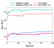
(a) CIFAR-10-LT

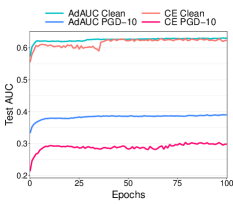
(b) CIFAR-100-LT

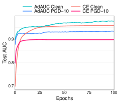
(c) MNIST-LT

Figure 3: The convergence of AUC on testing data of CIFAR-10-LT, CIFAR-100-LT and MNIST-LT.

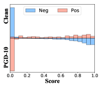
(a) CE NT

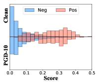
(b) CE AT₂

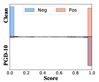
(c) AdAUC NT

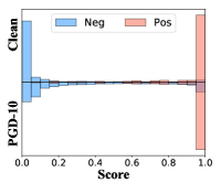
(d) AdAUC AT₂

Figure 4: Score distribution of positive and negative examples on MNIST-LT dataset. In each subfigure, the above part represents the score distribution evaluated against clean data, and the below part represents the score distribution evaluated against PGD-10.

Binary CIFAR-100-LT Dataset. We construct a long-tail CIFAR-100 dataset in the same way as CIFAR-10-LT, where we label the first 50 classes as the negative class and the last 50 classes as positive, which leads that the ratio of positive class size to negative class size $\rho\approx 1:9$.

Binary MNIST-LT Dataset. We construct a long-tail MNIST dataset from original MNIST dataset (LeCun et al., 1998) in the same way as CIFAR-10-LT, where the ratio of positive class size to negative class size $\rho\approx 1:9$.

5.3 Overall Performance

The performance and robustness of all the involved methods on three datasets are shown in Tab.2. Consequently, we have the following observations: 1) On all the datasets, our methods achieve the best or competitive performance evaluated against all adversarial attack methods as shown in Tab.2. 2) Even the AUC optimization with NT has certain robustness (the AUC will not drop to 0 when evaluated against adversarial examples). This is because the decision surface obtained by AUC optimization has a greater tolerance for minority classes than CE. Specifically, the decision surface is far away from the positive examples. To validate this argument, we show the score distribution in Fig.4 w.r.t MNIST-LT. For AdAUC NT, adversarial examples increase the score of the negative examples, while it has less impact on the positive examples. However, the perturbation becomes much more violent. As shown in Fig.4-(a), the adversarial examples simultaneously increase the score of the negative examples and decreases the score of the positive examples. The more results of other datasets are shown in the App.C.2, which show a similar trend. Moreover, we show the feature visualization of NT and AT₂ of our methods for clean data and adversarial examples. It implies that our AdAUC algorithm could separate the positive and negative instances well in the embedding space in Fig.2.

5.4 Convergence Analysis

We report the convergence of test AUC of CE-based methods and our proposed methods in Fig. 3. We can observe that our proposed method performs better both on clean data and adversarial examples. However, due to the high complexity of the outer min-max problem, it could be seen that our method converges slightly slower than CE methods, which is consistent with the analysis of Thm.2.

6 Conclusion

In this paper, we initiate the study on adversarial AUC optimization against long-tail problem. The complexity of AUC loss function makes the corresponding adversarial training hardly scalable. To address this issue, we first construct a reformulation of the AT problem of AUC optimization. By further applying a concavity promoting regularizer, we can reformulate the original problem as a min-max problem where the objective function can be expressed instance-wisely. On top of the reformulation, we construct an end-to-end training algorithm with provable guarantee. Finally, we conduct a series of empirical studies on three long-tail benchmark datasets, the results of which demonstrate the effectiveness of our proposed method.

Appendix A Proofs of Main Results

In this section, we provide the proofs of the main results.

A.1 Proof of Proposition 2

Proof.

According to (Ying et al., 2016), $a,b,\alpha$ have the following closed-form solution:

$$a=\hat{\mathbb{E}}[h_{\theta}(\bm{x})|y=1],~{}~{}b=\hat{\mathbb{E}}[h_{\theta}(\bm{x})|y=0],~{}~{}\alpha=\hat{\mathbb{E}}[h_{\theta}(\bm{x})|y=0]-\hat{\mathbb{E}}[h_{\theta}(\bm{x})|y=1].$$

Then it is easy to check that

$$r(a,b)=\max_{\alpha}\frac{1}{n}\sum^{n}_{i=1}g(\bm{\theta},a,b,\alpha,(\bm{x}_{i}+\bm{\delta}_{i},y_{i}))$$

is a strongly-convex problem w.r.t. $(a,b)$. However, $r$ is in general not concave w.r.t. $\bm{\delta}_{i}$. In this sense, we then try to find a surrogate objective to induce the concavity w.r.t $\bm{\delta}_{i}$. Specifically, we adopt a concavity regularization term $-\gamma||\bm{x}_{i}+\bm{\delta}_{i}||^{2}_{2}$, and define a surrogate objective:

$$f(\bm{w},\alpha,\bm{x}_{i}+\bm{\delta}_{i})=g(\bm{\theta},a,b,\alpha,(\bm{x}_{i}+\bm{\delta}_{i},y_{i}))-\gamma\left\|\bm{x}_{i}+\bm{\delta}_{i}\right\|^{2}_{2}.$$

Therefore, if $r$ is $\gamma_{\star}$-weakly concave w.r.t. $\bm{\delta}_{i},i=1,2,\cdots,n$ (Liu et al., 2021; Böhm & Wright, 2021), then we can define $\gamma>\gamma_{\star}$ to obtain an objective $f(\bm{w},\alpha,\bm{x}+\bm{\delta})$ such that $\max_{\alpha}\frac{1}{n}\sum^{n}_{i=1}f(\bm{w},\alpha,\bm{x}_{i}+\bm{\delta}_{i})$ is strongly concave w.r.t. $\bm{\delta}_{i},i=1,2,\cdots,n$. Above all, with the weakly concavity assumption, we can instead solve the following surrogate problem by the von Neumann’s minimax theorem:

(OP) $$\min\limits_{\bm{w}}\max\limits_{\alpha}\max\limits_{\bm{\delta}}\frac{1}{n}\sum^{n}_{i=1}\left[f(\bm{w},\alpha,\bm{x}_{i}+\bm{\delta}_{i})\right]$$ (7)

$$=\min\limits_{\bm{w}}\max\limits_{\alpha}\frac{1}{n}\sum^{n}_{i=1}\max\limits_{\bm{\delta}_{i}}\left[f(\bm{w},\alpha,\bm{x}_{i}+\bm{\delta}_{i})\right],$$

where $\bm{w}=(\bm{\theta},a,b)$. ∎

A.2 Proof of Lemma 1

Lemma 1.

For all $x\in\mathcal{X}$, $c(\bm{x}^{k})=0$ when 1) $\nabla_{\bm{x}}f(\bm{w},\alpha,\bm{x}^{k})=0$, or 2) $\bm{x}^{k}-\bm{x}^{0}=\epsilon\cdot\operatorname{sign}(\nabla_{\bm{x}}f(\bm{w},\alpha,\bm{x}^{k}))$.

Proof.

$$c(\bm{x}^{k}) =\max\limits_{\bm{x}\in\mathcal{X}}\langle\bm{x}-\bm{x}^{k},\nabla_{\bm{x}}f(\bm{w},\alpha,\bm{x}^{k})\rangle$$ (8)

$$=\max\limits_{\bm{x}\in\mathcal{X}}\langle\bm{x}-\bm{x}^{0}+\bm{x}^{0}-\bm{x}^{k},\nabla_{\bm{x}}f(\bm{w},\alpha,\bm{x}^{k})\rangle$$

$$=\max\limits_{\bm{x}\in\mathcal{X}}\langle\bm{x}-\bm{x}^{0},\nabla_{\bm{x}}f(\bm{w},\alpha,\bm{x}^{k})\rangle-\langle\bm{x}^{k}-\bm{x}^{0},\nabla_{\bm{x}}f(\bm{w},\alpha,\bm{x}^{k})\rangle$$

$$=\epsilon\cdot\left\|\nabla_{\bm{x}}f(\bm{w},\alpha,\bm{x}^{k})\right\|_{1}-\langle\bm{x}^{k}-\bm{x}^{0},\nabla_{\bm{x}}f(\bm{w},\alpha,\bm{x}^{k})\rangle$$

This completes the proof. ∎

A.3 Proof of Technical Lemmas

In this subsections, we present seven key lemmas which are important for the proof of Theorem 2.

Lemma 2.

Under the Asm.1 and 3, we have $L(\alpha)$ is $L_{\alpha}$-smooth where $L_{\alpha}=\frac{L_{\alpha x}L_{x\alpha}}{\mu}+L_{\alpha\alpha}$. For any $\alpha_{1},\alpha_{2}$, it holds

$$L(\alpha_{1})\leq L(\alpha_{2})+\langle\nabla L(\alpha_{2}),\alpha_{1}-\alpha_{2}\rangle+\frac{L_{\alpha}}{2}\left\|\alpha_{1}-\alpha_{2}\right\|^{2}_{2}$$ (9)

$$\left\|\nabla L(\alpha_{1})-\nabla L(\alpha_{2})\right\|_{2}\leq L_{\alpha}\left\|\alpha_{1}-\alpha_{2}\right\|_{2}.$$

We also have that $L(\bm{w})$ is $L_{w}$-smooth where $L_{w}=\frac{L_{wx}L_{xw}}{\mu}+L_{ww}$.

Proof.

Here, since we only focus on $\alpha$ and $\bm{x}$ when the $w$ is fixed, we abbreviate $\bm{x}^{*}(w,\alpha)$ as $\bm{x}^{*}(\alpha)$ for convenience.

By the Asm.3, we have

$$f(\bm{w},\alpha_{2},\bm{x}^{*}_{i}(\alpha_{1}))\leq f(\bm{w},\alpha_{2},\bm{x}^{*}_{i}(\alpha_{2}))+\langle\nabla_{\bm{x}}f(\bm{w},\alpha_{2},\bm{x}^{*}_{i}(\alpha_{2})),\bm{x}^{*}_{i}(\alpha_{1})-\bm{x}^{*}_{i}(\alpha_{2})\rangle-\frac{\mu}{2}\left\|\bm{x}^{*}_{i}(\alpha_{1})-\bm{x}^{*}_{i}(\alpha_{2})\right\|^{2}_{2},$$ (10)

$$f(\bm{w},\alpha_{2},\bm{x}^{*}_{i}(\alpha_{2}))\leq f(\bm{w},\alpha_{2},\bm{x}^{*}_{i}(\alpha_{1}))+\langle\nabla_{\bm{x}}f(\bm{w},\alpha_{2},\bm{x}^{*}_{i}(\alpha_{1})),\bm{x}^{*}_{i}(\alpha_{2})-\bm{x}^{*}_{i}(\alpha_{1})\rangle-\frac{\mu}{2}\left\|\bm{x}^{*}_{i}(\alpha_{1})-\bm{x}^{*}_{i}(\alpha_{2})\right\|^{2}_{2}.$$ (11)

Since $\langle\nabla_{\bm{x}}f(\bm{w},\alpha_{2},\bm{x}^{*}_{i}(\alpha_{2})),\bm{x}^{*}_{i}(\alpha_{1})-\bm{x}^{*}_{i}(\alpha_{2})\rangle\leq 0$, combining (10) and (11), we obtain

$$\mu\left\|\bm{x}^{*}_{i}(\alpha_{1})-\bm{x}^{*}_{i}(\alpha_{2})\right\|_{2}^{2} \leq\langle\nabla_{\bm{x}}f(\bm{w},\alpha_{2},\bm{x}^{*}_{i}(\alpha_{1})),\bm{x}^{*}_{i}(\alpha_{2})-\bm{x}^{*}_{i}(\alpha_{1})\rangle$$ (12)

$$\leq\langle\nabla_{\bm{x}}f(\bm{w},\alpha_{2},\bm{x}^{*}_{i}(\alpha_{1}))-\nabla_{\bm{x}}f(\bm{w},\alpha_{1},\bm{x}^{*}_{i}(\alpha_{1})),\bm{x}^{*}_{i}(\alpha_{2})-\bm{x}^{*}_{i}(\alpha_{1})\rangle$$

$$\leq\left\|\nabla_{\bm{x}}f(\bm{w},\alpha_{2},\bm{x}^{*}_{i}(\alpha_{1}))-\nabla_{\bm{x}}f(\bm{w},\alpha_{1},\bm{x}^{*}_{i}(\alpha_{1}))\right\|_{2}\left\|\bm{x}^{*}_{i}(\alpha_{2})-\bm{x}^{*}_{i}(\alpha_{1})\right\|_{2}$$

$$\leq L_{x\alpha}\left\|\alpha_{1}-\alpha_{2}\right\|_{2}\left\|\bm{x}^{*}_{i}(\alpha_{1})-\bm{x}^{*}_{i}(\alpha_{2})\right\|_{2},$$

where the second inequality holds because $\langle\nabla_{\bm{x}}f(\bm{w},\alpha_{1},\bm{x}^{*}_{i}(\alpha_{1})),\bm{x}^{*}_{i}(\alpha_{2})-\bm{x}^{*}_{i}(\alpha_{1})\rangle\leq 0$.

Then (12) immediately yields

$$\left\|\bm{x}^{*}_{i}(\alpha_{1})-\bm{x}^{*}_{i}(\alpha_{2})\right\|_{2}\leq\frac{L_{x\alpha}}{\mu}\left\|\alpha_{1}-\alpha_{2}\right\|_{2}.$$ (13)

Then for $i\in[n]$, we have

$$\left\|\nabla_{\alpha}f(\bm{w},\alpha_{1},\bm{x}^{*}_{i}(\alpha_{1}))-\nabla_{\alpha}f(\bm{w},\alpha_{2},\bm{x}^{*}_{i}(\alpha_{2}))\right\|_{2} \leq\left\|\nabla_{\alpha}f(\bm{w},\alpha_{1},\bm{x}^{*}_{i}(\alpha_{1}))-\nabla_{\alpha}f(\bm{w},\alpha_{1},\bm{x}^{*}_{i}(\alpha_{2}))\right\|_{2}$$ (14)

$$\ \ \ \ \ \ \ +\left\|\nabla_{\alpha}f(\bm{w},\alpha_{1},\bm{x}^{*}_{i}(\alpha_{2}))-\nabla_{\alpha}f(\bm{w},\alpha_{2},\bm{x}^{*}_{i}(\alpha_{2}))\right\|_{2}$$

$$\leq L_{\alpha x}\left\|\bm{x}^{*}_{i}(\alpha_{1})-\bm{x}^{*}_{i}(\alpha_{2})\right\|_{2}+L_{\alpha\alpha}\left\|\alpha_{1}-\alpha_{2}\right\|_{2}$$

$$\leq\left(\frac{L_{\alpha x}L_{x\alpha}}{\mu}+L_{\alpha\alpha}\right)\left\|\alpha_{1}-\alpha_{2}\right\|_{2}.$$

Finally, by the definition of $L(\alpha)$, we have

$$\left\|\nabla L(\alpha_{1})-\nabla L(\alpha_{2})\right\|_{2} \leq\left\|\frac{1}{n}\sum_{i=1}^{n}\nabla_{\alpha}f(\bm{w},\alpha_{1},\bm{x}^{*}_{i}(\alpha_{1}))-\frac{1}{n}\sum_{i=1}^{n}\nabla_{\alpha}f(\bm{w},\alpha_{2},\bm{x}^{*}_{i}(\alpha_{2}))\right\|_{2}$$ (15)

$$\leq\frac{1}{n}\sum_{i=1}^{n}\left\|\nabla_{\alpha}f(\bm{w},\alpha_{1},\bm{x}^{*}_{i}(\alpha_{1}))-\nabla_{\alpha}f(\bm{w},\alpha_{2},\bm{x}^{*}_{i}(\alpha_{2}))\right\|_{2}$$

$$\leq\left(\frac{L_{\alpha x}L_{x\alpha}}{\mu}+L_{\alpha\alpha}\right)\left\|\alpha_{1}-\alpha_{2}\right\|_{2}.$$

This completes the proof. ∎

Lemma 3.

Under the Asm.1, we have $\Phi(\bm{w})$ is $L_{w}$-smooth where$L_{w}=\frac{L_{w\alpha}L_{\alpha w}}{\mu}+L_{ww}$. For any $\bm{w}_{1},\bm{w}_{2}$, it holds

$$\Phi(\bm{w}_{1})\leq\Phi(\bm{w}_{2})+\langle\nabla\Phi(\bm{w}_{2}),\bm{w}_{1}-\bm{w}_{2}\rangle+\frac{L_{w}}{2}\left\|\bm{w}_{1}-\bm{w}_{2}\right\|^{2}_{2}$$ (16)

$$\left\|\nabla\Phi(\bm{w}_{1})-\nabla\Phi(\bm{w}_{2})\right\|_{2}\leq L_{w}\left\|\bm{w}_{1}-\bm{w}_{2}\right\|_{2}.$$

Proof.

By the Rem.1, we have

$$L(\bm{w}_{2},\alpha^{*}(\bm{w}_{1}))\leq L(\bm{w}_{2},\alpha^{*}(\bm{w}_{2}))+\langle\nabla_{\alpha}L(\bm{w}_{2},\alpha^{*}(\bm{w}_{2})),\alpha^{*}(\bm{w}_{1})-\alpha^{*}(\bm{w}_{2})\rangle-\frac{\mu}{2}\left\|\alpha^{*}(\bm{w}_{1})-\alpha^{*}(\bm{w}_{2})\right\|^{2}_{2},$$ (17)

$$L(\bm{w}_{2},\alpha^{*}(\bm{w}_{2}))\leq L(\bm{w}_{2},\alpha^{*}(\bm{w}_{1}))+\langle\nabla_{\alpha}L(\bm{w}_{2},\alpha^{*}(\bm{w}_{1})),\alpha^{*}(\bm{w}_{2})-\alpha^{*}(\bm{w}_{1})\rangle-\frac{\mu}{2}\left\|\alpha^{*}(\bm{w}_{1})-\alpha^{*}(\bm{w}_{2})\right\|^{2}_{2}.$$ (18)

Since $\langle\nabla_{\alpha}L(\bm{w}_{2},\alpha^{*}(\bm{w}_{2})),\alpha^{*}(\bm{w}_{1})-\alpha^{*}(\bm{w}_{2})\rangle\leq 0$, combining (17) and (18), we obtain

$$\mu\left\|\alpha^{*}(\bm{w}_{1})-\alpha^{*}(\bm{w}_{2})\right\|_{2}^{2} \leq\langle\nabla_{\alpha}L(\bm{w}_{2},\alpha^{*}(\bm{w}_{1})),\alpha^{*}(\bm{w}_{2})-\alpha^{*}(\bm{w}_{1})\rangle$$ (19)

$$\leq\langle\nabla_{\alpha}L(\bm{w}_{2},\alpha^{*}(\bm{w}_{1}),)-\nabla_{\alpha}L(\bm{w}_{1},\alpha^{*}(\bm{w}_{1})),\alpha^{*}(\bm{w}_{2})-\alpha^{*}(\bm{w}_{1})\rangle$$

$$\leq\left\|\nabla_{\alpha}L(\bm{w}_{2},\alpha^{*}(\bm{w}_{1}))-\nabla_{\alpha}L(\bm{w}_{1},\alpha^{*}(\bm{w}_{1}))\right\|_{2}\left\|\alpha^{*}(\bm{w}_{2})-\alpha^{*}(\bm{w}_{1})\right\|_{2}$$

$$\leq L_{\alpha w}\left\|\bm{w}_{2}-\bm{w}_{1}\right\|_{2}\left\|\alpha^{*}(\bm{w}_{2})-\alpha^{*}(\bm{w}_{1})\right\|_{2}.$$

Then (19) yields

$$\left\|\alpha^{*}(\bm{w}_{1})-\alpha^{*}(\bm{w}_{2})\right\|_{2}\leq\frac{L_{\alpha w}}{\mu}\left\|\bm{w}_{1}-\bm{w}_{2}\right\|_{2}.$$ (20)

Then we have for $i\in[n]$,

$$\left\|\nabla_{\bm{w}}L(\bm{w}_{1},\alpha^{*}(\bm{w}_{1}))-\nabla_{\bm{w}}L(\bm{w}_{2},\alpha^{*}(\bm{w}_{2}))\right\|_{2} \leq\left\|\nabla_{\bm{w}}L(\bm{w}_{1},\alpha^{*}(\bm{w}_{1})))-\nabla_{\bm{w}}L(\bm{w}_{1},\alpha^{*}(\bm{w}_{2}))\right\|_{2}$$ (21)

$$\ \ \ \ \ \ \ +\left\|\nabla_{\bm{w}}L(\bm{w}_{1},\alpha^{*}(\bm{w}_{2}))-\nabla_{\bm{w}}L(\bm{w}_{2},\alpha^{*}(\bm{w}_{1}))\right\|_{2}$$

$$\leq L_{w\alpha}\left\|\alpha^{*}(\bm{w}_{1})-\alpha^{*}(\bm{w}_{2})\right\|_{2}+L_{ww}\left\|\bm{w}_{1}-\bm{w}_{2}\right\|_{2}$$

$$\leq\big{(}\frac{L_{w\alpha}L_{\alpha w}}{\mu}+L_{ww}\big{)}\left\|\bm{w}_{1}-\bm{w}_{2}\right\|_{2}.$$

Finally, by the definition of $\Phi(\bm{w})$, we have

$$\left\|\nabla\Phi(\bm{w}_{1})-\nabla\Phi(\bm{w}_{2})\right\|_{2} \leq\left\|\frac{1}{n}\sum_{i=1}^{n}\nabla_{\bm{w}}L(\bm{w}_{1},\alpha^{*}(\bm{w}_{1}))-\frac{1}{n}\sum_{i=1}^{n}\nabla_{\bm{w}}L(\bm{w}_{2},\alpha^{*}(\bm{w}_{2}))\right\|_{2}$$ (22)

$$\leq\frac{1}{n}\sum_{i=1}^{n}\left\|\nabla_{\alpha}L(\bm{w}_{1},\alpha^{*}(\bm{w}_{1}))-\nabla_{\alpha}L(\bm{w}_{2},\alpha^{*}(\bm{w}_{2}))\right\|_{2}$$

$$\leq\big{(}\frac{L_{w\alpha}L_{\alpha w}}{\mu}+L_{ww}\big{)}\left\|\bm{w}_{1}-\bm{w}_{2}\right\|_{2}.$$

This completes the proof. ∎

Lemma 4.

Under Asm.1 and 3, the approximate stochastic gradient $\hat{g}(\alpha)$ satisfies

$$\left\|\hat{g}(\alpha)-g(\alpha)\right\|_{2}\leq L_{\alpha x}\sqrt{\frac{\delta}{\mu}}.$$ (23)

We also have

$$\left\|\hat{g}(\bm{w})-g(\bm{w})\right\|_{2}\leq L_{wx}\sqrt{\frac{\delta}{\mu}}.$$ (24)

Proof.

We have

$$\left\|\hat{g}(\alpha)-g(\alpha)\right\|_{2} \leq\left\|\frac{1}{|\mathcal{B}|}\sum_{i\in\mathcal{B}}\big{(}\nabla_{\alpha}f(\bm{w},\alpha,\hat{\bm{x}}_{i}(\alpha))-\nabla_{\alpha}f(\bm{w},\alpha,\bm{x}^{*}_{i}(\alpha))\big{)}\right\|_{2}$$ (25)

$$\leq\frac{1}{|\mathcal{B}|}\sum_{i\in\mathcal{B}}\left\|\nabla_{\alpha}f(\bm{w},\alpha,\hat{\bm{x}}_{i}(\alpha))-\nabla_{\alpha}f(\bm{w},\alpha,\bm{x}^{*}_{i}(\alpha))\right\|_{2}$$

$$\leq\frac{1}{|\mathcal{B}|}\sum_{i\in\mathcal{B}}L_{\alpha x}\left\|\hat{\bm{x}}_{i}(\alpha)-\bm{x}^{*}_{i}(\alpha)\right\|_{2}.$$

By the Asm.3, we have

$$\mu\left\|\hat{\bm{x}}_{i}(\alpha)-\bm{x}^{*}_{i}(\alpha)\right\|_{2}^{2}\leq\langle\nabla_{\alpha}f(\bm{w},\alpha,\hat{\bm{x}}_{i}(\alpha))-\nabla_{\alpha}f(\bm{w},\alpha,\bm{x}^{*}_{i}(\alpha)),\hat{\bm{x}}_{i}(\alpha)-\bm{x}^{*}_{i}(\alpha)\rangle.$$ (26)

Since the $\hat{\bm{x}}_{i}(\alpha)$ is a $\delta$-approximate solution to $\bm{x}^{*}_{i}(\alpha)$, if it satisfies that

$$\langle\bm{x}^{*}_{i}(\alpha)-\hat{\bm{x}}_{i}(\alpha),\nabla_{\bm{x}}f(\bm{w},\alpha,\hat{\bm{x}}_{i}(\alpha)\rangle\leq\delta.$$ (27)

Furthermore, we have

$$\langle\hat{\bm{x}}_{i}(\alpha)-\bm{x}^{*}_{i}(\alpha),\nabla_{\bm{x}}f(\bm{w},\alpha,\bm{x}^{*}_{i}(\alpha))\rangle\leq 0.$$ (28)

Combining (27) and (28), we obtain

$$\langle\hat{\bm{x}}_{i}(\alpha)-\bm{x}^{*}_{i}(\alpha),\nabla_{\bm{x}}f(\bm{w},\alpha,\bm{x}^{*}_{i}(\alpha))-\nabla_{\bm{x}}f(\alpha,\hat{\bm{x}}_{i})(\alpha)\rangle\leq\delta.$$ (29)

Combining (26) and (29), we obtain

$$\mu\left\|\hat{\bm{x}}_{i}(\alpha)-\bm{x}^{*}_{i}(\alpha)\right\|_{2}^{2}\leq\delta$$ (30)

Combining (25) and (30), we obtain

$$\left\|\hat{g}(\alpha)-g(\alpha)\right\|_{2}\leq L_{\alpha x}\sqrt{\frac{\delta}{\mu}}.$$ (31)

∎

Lemma 5.

$g(\bm{w})=\frac{1}{M}\sum_{i=1}^{M}G_{w}(\bm{w}_{t},\alpha_{t},\xi_{i})$ and $g(\alpha)=\frac{1}{M}\sum_{i=1}^{M}G_{\alpha}(\bm{w}_{t},\alpha_{t},\xi_{i})$ are unbiased and have bounded variance:

$$\mathbb{E}[g(\bm{w})]=\nabla_{\bm{w}}L(\bm{w}_{t},\alpha_{t}), \mathbb{E}\left[\left\|g(\bm{w})\right\|_{2}^{2}\right]=\left\|\nabla_{\bm{w}}L(\bm{w}_{t},\alpha_{t})\right\|^{2}_{2}+\frac{\sigma^{2}}{M},$$ (32)

$$\mathbb{E}[g(\alpha)]=\nabla_{\alpha}L(\bm{w}_{t},\alpha_{t}), \mathbb{E}\left[\left\|g(\alpha)\right\|_{2}^{2}\right]=\left\|\nabla_{\alpha}L(\bm{w}_{t},\alpha_{t})\right\|^{2}_{2}+\frac{\sigma^{2}}{M}.$$

Proof.

Since $\hat{g}$ is unbiased, we have

$$\mathbb{E}[g(\bm{w})]=\nabla_{\bm{w}}L(\bm{w}_{t},\alpha_{t}), \mathbb{E}[g(\alpha)]=\nabla_{\alpha}L(\bm{w}_{t},\alpha_{t}).$$

Furthermore, we have

$$\mathbb{E}[\left\|g(\bm{w})-\nabla_{\bm{w}}L(\bm{w}_{t},\alpha_{t})\right\|_{2}^{2}] =\mathbb{E}\left[\left\|\frac{1}{M}\sum_{i=1}^{M}G_{w}(\bm{w}_{t},\alpha_{t},\xi_{i})-\nabla_{\bm{w}}L(\bm{w}_{t},\alpha_{t})\right\|^{2}_{2}\right]$$

$$=\frac{\sum_{i=1}^{M}\mathbb{E}\left[\left\|G_{w}(\bm{w}_{t},\alpha_{t},\xi_{i})-\nabla_{\bm{w}}L(\bm{w}_{t},\alpha_{t})\right\|_{2}^{2}\right]}{M^{2}} \leq\frac{\sigma^{2}}{M}.$$

$$\mathbb{E}[\left\|g(\alpha)-\nabla_{\alpha}L(\bm{w}_{t},\alpha_{t})\right\|_{2}^{2}] =\mathbb{E}\left[\left\|\frac{1}{M}\sum_{i=1}^{M}G_{\alpha}(\bm{w}_{t},\alpha_{t},\xi_{i})-\nabla_{\alpha}L(\bm{w}_{t},\alpha_{t})\right\|^{2}_{2}\right]$$

$$=\frac{\sum_{i=1}^{M}\mathbb{E}\left[\left\|G_{\alpha}(\bm{w}_{t},\alpha_{t},\xi_{i})-\nabla_{\alpha}L(\bm{w}_{t},\alpha_{t})\right\|_{2}^{2}\right]}{M^{2}} \leq\frac{\sigma^{2}}{M}.$$

∎

Lemma 6.

The iterates $\{\bm{w}_{t}\}_{t\geq 1}$ satisfy the following inequality:

$$\mathbb{E}[\Phi(\bm{w}_{t})] \leq\mathbb{E}[\Phi(\bm{w}_{t-1})]-\left(\frac{\eta_{w}}{2}-2L_{w}\eta_{w}^{2}\right)\mathbb{E}\left[\left\|\nabla\Phi(\bm{w}_{t-1})\right\|_{2}^{2}\right]$$ (33)

$$\ \ \ \ \ +(\frac{\eta_{w}}{2}+2L_{w}\eta_{w}^{2})\mathbb{E}\left[\left\|\nabla\Phi(\bm{w}_{t-1})-\nabla_{\bm{w}}L(\bm{w}_{t-1},\alpha_{t-1})\right\|_{2}^{2}\right]+\frac{L_{w}\eta_{w}^{2}\sigma^{2}}{M}+\frac{\delta L_{w}L_{wx}^{2}\eta_{w}^{2}}{\mu}+L_{wx}\ell_{w}\sqrt{\frac{\delta}{\mu}}.$$

Proof.

By Lem.2, we have

$$\Phi(\bm{w}_{t})\leq\Phi(\bm{w}_{t-1})+\langle\nabla\Phi(\bm{w}_{t-1}),\bm{w}_{t}-\bm{w}_{t-1}\rangle+\frac{L_{w}}{2}\left\|\bm{w}_{t}-\bm{w}_{t-1}\right\|_{2}^{2}.$$ (34)

Plugging $\bm{w}_{t}-\bm{w}_{t-1}=-\eta_{w}\hat{g}(\bm{w})$ into (34) yields that

$$\Phi(\bm{w}_{t}) \leq\Phi(\bm{w}_{t-1})-\eta_{w}\langle\nabla\Phi(\bm{w}_{t-1}),\hat{g}(\bm{w})\rangle+\frac{L_{w}\eta_{w}^{2}}{2}\left\|\hat{g}(\bm{w})\right\|_{2}^{2}$$ (35)

$$=\Phi(\bm{w}_{t-1})-\eta_{w}\left\|\nabla\Phi(\bm{w}_{t-1})\right\|_{2}^{2}-\eta_{w}\langle\nabla\Phi(\bm{w}_{t-1}),\hat{g}(\bm{w})-\nabla\Phi(\bm{w}_{t-1})\rangle+\frac{L_{w}\eta_{w}^{2}}{2}\left\|\hat{g}(\bm{w})\right\|_{2}^{2}$$

$$\leq\Phi(\bm{w}_{t-1})-\eta_{w}\left\|\nabla\Phi(\bm{w}_{t-1})\right\|_{2}^{2}-\eta_{w}\langle\nabla\Phi(\bm{w}_{t-1}),g(\bm{w})-\nabla\Phi(\bm{w}_{t-1})\rangle+L_{w}\eta_{w}^{2}\left\|g(\bm{w})\right\|_{2}^{2}$$

$$\ \ \ \ \ +L_{w}\eta_{w}^{2}\left\|\hat{g}(\bm{w})-g(\bm{w})\right\|_{2}^{2}-\eta_{w}\langle\nabla\Phi(\bm{w}_{t-1}),\hat{g}(\bm{w})-g(\bm{w})\rangle$$

$$=\Phi(\bm{w}_{t-1})-\eta_{w}\left\|\nabla\Phi(\bm{w}_{t-1})\right\|_{2}^{2}-\eta_{w}\langle\nabla\Phi(\bm{w}_{t-1}),g(\bm{w})-\nabla_{\bm{w}}L(\bm{w}_{t-1},\alpha_{t-1})\rangle$$

$$\ \ \ \ \ -\eta_{w}\langle\nabla\Phi(\bm{w}_{t-1}),\nabla_{\bm{w}}L(\bm{w}_{t-1},\alpha_{t-1})-\nabla\Phi(\bm{w}_{t-1})\rangle+L_{w}\eta_{w}^{2}\left\|g(\bm{w})\right\|_{2}^{2}$$

$$\ \ \ \ \ +L_{w}\eta_{w}^{2}\left\|\hat{g}(\bm{w})-g(\bm{w})\right\|_{2}^{2}-\eta_{w}\langle\nabla\Phi(\bm{w}_{t-1}),\hat{g}(\bm{w})-g(\bm{w})\rangle$$

$$\leq\Phi(\bm{w}_{t-1})-\frac{\eta_{w}}{2}\left\|\nabla\Phi(\bm{w}_{t-1})\right\|_{2}^{2}-\eta_{w}\langle\nabla\Phi(\bm{w}_{t-1}),g(\bm{w})-\nabla_{\bm{w}}L(\bm{w}_{t-1},\alpha_{t-1})\rangle$$

$$\ \ \ \ \ +\frac{\eta_{w}}{2}\left\|\nabla\Phi(\bm{w}_{t-1})-\nabla_{\bm{w}}L(\bm{w}_{t-1},\alpha_{t-1})\right\|_{2}^{2}+L_{w}\eta_{w}^{2}\left\|g(\bm{w})\right\|_{2}^{2}+\frac{\delta L_{w}L_{wx}^{2}\eta_{w}^{2}}{\mu}+\eta_{w}L_{wx}\ell_{w}\sqrt{\frac{\delta}{\mu}}.$$

By Lem.5, taking an expectation on the both sides yields that,

$$\mathbb{E}\left[\Phi(\bm{w}_{t})\right] \leq\mathbb{E}[\Phi(\bm{w}_{t-1})]-\frac{\eta_{w}}{2}\mathbb{E}\left[\left\|\nabla\Phi(\bm{w}_{t-1})\right\|_{2}^{2}\right]+\frac{\eta_{w}}{2}\mathbb{E}\left[\left\|\nabla\Phi(\bm{w}_{t-1})-\nabla_{\bm{w}}L(\bm{w}_{t-1},\alpha_{t-1})\right\|_{2}^{2}\right]$$ (36)

$$\ \ \ \ \ +L_{w}\eta_{w}^{2}\left\|\nabla_{\bm{w}}L(\bm{w}_{t-1},\alpha_{t-1})\right\|_{2}^{2}+\frac{L_{w}\eta_{w}^{2}\sigma^{2}}{M}+\frac{\delta L_{w}L_{wx}^{2}\eta_{w}^{2}}{\mu}+\eta_{w}L_{wx}\ell_{w}\sqrt{\frac{\delta}{\mu}}.$$

By the Cauchy-Schwartz inequality, we have

$$\left\|\nabla_{\bm{w}}L(\bm{w}_{t-1},\alpha_{t-1})\right\|_{2}^{2}\leq 2\left(\left\|\nabla_{\bm{w}}L(\bm{w}_{t-1},\alpha_{t-1})-\nabla\Phi(\bm{w}_{t-1})\right\|_{2}^{2}+\left\|\nabla\Phi(\bm{w}_{t-1})\right\|_{2}^{2}\right).$$ (37)

Plugging (37) into (36) and taking the expectation of both side, yields that

$$\mathbb{E}[\Phi(\bm{w}_{t})] \leq\mathbb{E}[\Phi(\bm{w}_{t-1})]-\left(\frac{\eta_{w}}{2}-2L_{w}\eta_{w}^{2}\right)\mathbb{E}\left[\left\|\nabla\Phi(\bm{w}_{t-1})\right\|_{2}^{2}\right]$$

$$\ \ \ \ \ +\left(\frac{\eta_{w}}{2}+2L_{w}\eta_{w}^{2}\right)\mathbb{E}\left[\left\|\nabla\Phi(\bm{w}_{t-1})-\nabla_{\bm{w}}L(\bm{w}_{t-1},\alpha_{t-1})\right\|_{2}^{2}\right]+\frac{L_{w}\eta_{w}^{2}\sigma^{2}}{M}+\frac{\delta L_{w}L_{wx}^{2}\eta_{w}^{2}}{\mu}+\eta_{w}L_{wx}\ell_{w}\sqrt{\frac{\delta}{\mu}}.$$

This completes the proof. ∎

Lemma 7.

let $\delta_{t}=\mathbb{E}\left[\left\|\alpha^{*}(\bm{w}_{t},x_{t}^{*})-\alpha_{t}(\bm{w}_{t},\hat{x}_{t})\right\|^{2}_{2}\right]$, the following statements holds that

$$\delta_{t}\leq \left(1-\frac{\mu}{2L_{\alpha w}}+\frac{L_{ww}^{2}L_{\alpha w}^{3}\eta_{w}^{2}}{2\mu^{3}}\right)\delta_{t-1}+\frac{L_{\alpha w}^{3}\eta_{w}^{2}}{4\mu^{3}}\mathbb{E}\left[\left\|\nabla\Phi(\bm{w}_{t-1})\right\|_{2}^{2}\right]$$

$$+\frac{2\sigma^{2}}{L_{\alpha w}^{2}M}+\frac{L_{\alpha w}^{3}\eta_{w}^{2}\sigma^{2}}{4\mu^{3}M}+\frac{L_{\alpha w}^{3}L_{wx}^{2}\eta_{w}^{2}\sigma^{2}}{4\mu^{4}}+\frac{L_{\alpha w}L_{\alpha x}^{2}\Delta}{8\mu^{3}}+\frac{2L_{\alpha x}^{2}\delta}{\mu^{3}}.$$

Proof.

$$\delta_{t} =\mathbb{E}\left[\left\|\alpha^{*}(\bm{w}_{t},x_{t}^{*})-\alpha^{*}(\bm{w}_{t},\hat{x}_{t})+\alpha^{*}(\bm{w}_{t},\hat{x}_{t})-\alpha_{t}(\bm{w}_{t},\hat{x}_{t})\right\|_{2}^{2}\right]$$ (38)

$$\leq 2\mathbb{E}\left[\left\|\alpha^{*}(\bm{w}_{t},x_{t}^{*})-\alpha^{*}(\bm{w}_{t},\hat{x}_{t})\right\|_{2}^{2}\right]+2\mathbb{E}\left[\left\|\alpha^{*}(\bm{w}_{t},\hat{x}_{t})-\alpha_{t}(\bm{w}_{t},\hat{x}_{t})\right\|_{2}^{2}\right].$$

By Young’s inequality, for any $\epsilon_{0}\leq 0$, we have

$$\mathbb{E}\left[\left\|\alpha^{*}(\bm{w}_{t},\hat{x}_{t})-\alpha_{t}(\bm{w}_{t},\hat{x}_{t})\right\|_{2}^{2}\right]\leq \left(1+\frac{1}{\epsilon_{0}}\right)\mathbb{E}\left[\left\|\alpha^{*}(\bm{w}_{t-1},\hat{x}_{t-1})-\alpha_{t}(\bm{w}_{t},\hat{x}_{t})\right\|_{2}^{2}\right]$$ (39)

$$+\left(1+\epsilon_{0}\right)\mathbb{E}\left[\left\|\alpha^{*}(\bm{w}_{t},\hat{x}_{t})-\alpha^{*}(\bm{w}_{t-1},\hat{x}_{t-1})\right\|_{2}^{2}\right].$$

By the Rem.1 and $\eta_{\alpha}=1/L_{\alpha w}$ (refer to (Nesterov, 1998) Theorem 2.3.4), we have

$$\mathbb{E}\left[\left\|\alpha^{*}(\bm{w}_{t-1},\hat{x}_{t})-\alpha_{t}(\bm{w}_{t},\hat{x}_{t})\right\|_{2}^{2}\right] \leq\left(1-\frac{\mu}{L_{\alpha w}}\right)\mathbb{E}\left[\left\|\alpha^{*}(\bm{w}_{t-1},\hat{x}_{t-1})-\alpha_{t-1}(\bm{w}_{t-1},\hat{x}_{t-1})\right\|_{2}^{2}\right]+\frac{\sigma^{2}}{L_{\alpha w}^{2}M}.$$ (40)

By triangle inequality, we have

$$\mathbb{E}\left[\left\|\alpha^{*}(\bm{w}_{t-1},\hat{x}_{t-1})-\alpha_{t-1}(\bm{w}_{t-1},\hat{x}_{t-1})\right\|_{2}^{2}\right]\leq 2\mathbb{E}\left[\left\|\alpha^{*}(\bm{w}_{t-1},\hat{x}_{t-1})-\alpha^{*}(\bm{w}_{t-1},x^{*}_{t-1})\right\|_{2}^{2}\right]$$ (41)

$$+2\mathbb{E}\left[\left\|\alpha^{*}(\bm{w}_{t-1},x^{*}_{t-1})-\alpha_{t-1}(\bm{w}_{t-1},\hat{x}_{t-1})\right\|_{2}^{2}\right].$$

Plugging (41) into (40), yields that

$$\mathbb{E}\left[\left\|\alpha^{*}(\bm{w}_{t-1},\hat{x}_{t-1})-\alpha_{t}(\bm{w}_{t},\hat{x}_{t})\right\|_{2}^{2}\right] \leq 2\left(1-\frac{\mu}{L_{\alpha w}}\right)\left[\delta_{t-1}+\mathbb{E}\left[\left\|\alpha^{*}(\bm{w}_{t-1},\hat{x}_{t-1})-\alpha^{*}(\bm{w}_{t-1},x^{*}_{t-1})\right\|_{2}^{2}\right]\right]+\frac{\sigma^{2}}{L_{\alpha w}^{2}M}.$$ (42)

By triangle inequality, we have

$$\mathbb{E}\left[\left\|\alpha^{*}(\bm{w}_{t},\hat{x}_{t})-\alpha^{*}(\bm{w}_{t-1},\hat{x}_{t-1})\right\|_{2}^{2}\right]\leq 2\mathbb{E}\left[\left\|\alpha^{*}(\bm{w}_{t},\hat{x}_{t})-\alpha^{*}(\bm{w}_{t-1},\hat{x}_{t})\right\|_{2}^{2}\right]$$ (43)

$$+2\mathbb{E}\left[\left\|\alpha^{*}(\bm{w}_{t-1},\hat{x}_{t})-\alpha^{*}(\bm{w}_{t-1},\hat{x}_{t-1})\right\|_{2}^{2}\right].$$

Since $\alpha^{*}(\cdot)$ is $\frac{L_{\alpha w}}{\mu}$-Lipschitz, we have

$$\mathbb{E}\left[\left\|\alpha^{*}(\bm{w}_{t},\hat{x}_{t})-\alpha^{*}(\bm{w}_{t-1},\hat{x}_{t})\right\|_{2}^{2}\right]\leq\frac{L_{\alpha w}^{2}}{\mu^{2}}\mathbb{E}\left[\left\|\bm{w}_{t}-\bm{w}_{t-1}\right\|^{2}_{2}\right].$$ (44)

Furthermore, we have

$$\mathbb{E}\left[\left\|\bm{w}_{t}-\bm{w}_{t-1}\right\|^{2}_{2}\right] =\eta_{w}^{2}\mathbb{E}\left[\left\|\hat{g}(\bm{w})\right\|_{2}^{2}\right]$$ (45)

$$=2\eta_{w}^{2}\mathbb{E}\left[\left\|g(\bm{w})\right\|_{2}^{2}\right]+2\eta_{w}^{2}\mathbb{E}\left[\left\|\hat{g}(\bm{w})-g(\bm{w})\right\|_{2}^{2}\right]$$

$$\leq 2\eta_{w}^{2}\left\|\nabla_{\bm{w}}L(\bm{w}_{t-1},\alpha_{t-1})\right\|_{2}^{2}+\frac{2\eta_{w}^{2}\sigma^{2}}{M}+\frac{2\delta L_{wx}^{2}\eta_{w}^{2}}{\mu}$$

$$\mathop{\leq}\limits^{(\ref{equ_lemma4_3})}4\eta_{w}^{2}\left(\left\|\nabla_{\bm{w}}L(\bm{w}_{t-1},\alpha_{t-1})-\nabla\Phi(\bm{w}_{t-1})\right\|_{2}^{2}+\left\|\nabla\Phi(\bm{w}_{t-1})\right\|_{2}^{2}\right)+\frac{2\eta_{w}^{2}\sigma^{2}}{M}+\frac{2\delta L_{wx}^{2}\eta_{w}^{2}}{\mu}$$

$$\leq 4L_{ww}^{2}\eta_{w}^{2}\delta_{t-1}+4\eta_{w}^{2}\left\|\nabla\Phi(\bm{w}_{t-1})\right\|_{2}^{2}+\frac{2\eta_{w}^{2}\sigma^{2}}{M}+\frac{2\delta L_{wx}^{2}\eta_{w}^{2}}{\mu}.$$

Plugging (44) and (45) into (43) and taking the exception of both side, yields that

$$\mathbb{E}\left[\left\|\alpha^{*}(\bm{w}_{t},\hat{x}_{t})-\alpha^{*}(\bm{w}_{t-1},\hat{x}_{t-1})\right\|_{2}^{2}\right] \leq\frac{8L_{\alpha w}^{2}L_{ww}^{2}\eta_{w}^{2}}{\mu^{2}}\delta_{t-1}+\frac{8L_{\alpha w}^{2}\eta_{w}^{2}}{\mu^{2}}\mathbb{E}\left[\left\|\nabla\Phi(\bm{w}_{t-1})\right\|_{2}^{2}\right]+\frac{4L_{\alpha w}^{2}\eta_{w}^{2}\sigma^{2}}{\mu^{2}M}$$ (46)

$$\ \ \ \ \ +\frac{4L_{\alpha w}^{2}L_{wx}^{2}\eta_{w}^{2}\delta}{\mu^{3}}+2\mathbb{E}\left[\left\|\alpha^{*}(\bm{w}_{t-1},\hat{x}_{t})-\alpha^{*}(\bm{w}_{t-1},\hat{x}_{t-1})\right\|_{2}^{2}\right].$$

Then, plugging (42) and (46) into (39) and let $\epsilon_{0}=\frac{8(\kappa-1)}{7-6\kappa}$ and $\kappa\leq\frac{7}{6}$, yields that

$$\mathbb{E}\left[\left\|\alpha^{*}(\bm{w}_{t},\hat{x}_{t})-\alpha_{t}(\bm{w}_{t},\hat{x}_{t})\right\|_{2}^{2}\right]\leq \left(\frac{1}{2}-\frac{\mu}{4L_{\alpha w}}+\frac{L_{ww}^{2}L_{\alpha w}^{3}\eta_{w}^{2}}{4\mu^{3}}\right)\delta_{t-1}+\frac{L_{\alpha w}^{3}\eta_{w}^{2}}{4\mu^{3}}\mathbb{E}\left[\left\|\nabla\Phi(\bm{w}_{t-1})\right\|_{2}^{2}\right]$$ (47)

$$+\frac{\sigma^{2}}{L_{\alpha w}^{2}M}+\frac{L_{\alpha w}^{3}\eta_{w}^{2}\sigma^{2}}{8\mu^{3}M}+\frac{L_{\alpha w}^{3}L_{wx}^{2}\eta_{w}^{2}\delta}{8\mu^{4}}$$

$$+\frac{L_{\alpha w}}{16\mu}\mathbb{E}\left[\left\|\alpha^{*}(\bm{w}_{t-1},\hat{x}_{t})-\alpha^{*}(\bm{w}_{t-1},\hat{x}_{t-1})\right\|_{2}^{2}\right].$$

Since $\alpha^{*}(\cdot)$ is $\frac{L_{\alpha x}}{\mu}$-Lipschitz, we have

$$\mathbb{E}\left[\left\|\alpha^{*}(\bm{w}_{t-1},\hat{x}_{t})-\alpha^{*}(\bm{w}_{t-1},\hat{x}_{t-1})\right\|_{2}^{2}\right]\leq\frac{L_{\alpha x}^{2}}{\mu^{2}}\mathbb{E}\left[\left\|\hat{x}_{t}-\hat{x}_{t-1}\right\|_{2}^{2}\right]\leq\frac{L_{\alpha x}^{2}}{\mu^{2}}\Delta,$$ (48)

$$\mathbb{E}\left[\left\|\alpha^{*}(\bm{w}_{t},x_{t}^{*})-\alpha^{*}(\bm{w}_{t},\hat{x}_{t})\right\|_{2}^{2}\right]\leq\frac{L_{\alpha x}^{2}}{\mu^{2}}\mathbb{E}\left[\left\|x^{*}_{t}-\hat{x}_{t}\right\|_{2}^{2}\right]\leq\frac{L_{\alpha x}^{2}\delta}{\mu^{3}},$$ (49)

where $\Delta$ is the maximum distance between two adversarial samples on the same sample. We can get the value of $\Delta$ by the diameter if $\mathcal{X}_{i}$.

Plugging (46) (47) and (48) into (38), yields that

$$\delta_{t}\leq \left(1-\frac{\mu}{2L_{\alpha w}}+\frac{L_{ww}^{2}L_{\alpha w}^{3}\eta_{w}^{2}}{2\mu^{3}}\right)\delta_{t-1}+\frac{L_{\alpha w}^{3}\eta_{w}^{2}}{4\mu^{3}}\mathbb{E}\left[\left\|\nabla\Phi(\bm{w}_{t-1})\right\|_{2}^{2}\right]$$

$$+\frac{2\sigma^{2}}{L_{\alpha w}^{2}M}+\frac{L_{\alpha w}^{3}\eta_{w}^{2}\sigma^{2}}{4\mu^{3}M}+\frac{L_{\alpha w}^{3}L_{wx}^{2}\eta_{w}^{2}\delta}{4\mu^{4}}+\frac{L_{\alpha w}L_{\alpha x}^{2}\Delta}{8\mu^{3}}+\frac{2L_{\alpha x}^{2}\delta}{\mu^{3}}.$$

∎

Lemma 8.

let $\delta_{t}=\mathbb{E}[\left\|\alpha^{*}(\bm{w}_{t},x_{t}^{*})-\alpha_{t}(\bm{w}_{t},\hat{x}_{t})\right\|^{2}_{2}]$, the following statements holds that

$$\mathbb{E}[\Phi(\bm{w}_{t})] \leq\mathbb{E}\left[\Phi(\bm{w}_{t-1})\right]-\frac{\eta_{w}}{4}\mathbb{E}\left[\left\|\nabla\Phi(\bm{w}_{t-1})\right\|_{2}^{2}\right]+\frac{3\eta_{w}L^{2}\delta_{t-1}}{4}+\frac{L_{w}\eta_{w}^{2}\sigma^{2}}{M}+\frac{\delta L_{w}L^{2}\eta_{w}^{2}}{\mu}+\eta_{w}L\ell_{w}\sqrt{\frac{\delta}{\mu}}.$$

Proof.

Let $\eta_{w}=\frac{1}{16(\kappa+1)^{2}L}$, where $L$ is the maximum value in the set $\{L_{ww},L_{w\alpha},L_{\alpha w},L_{xw},L_{wx},L_{x\alpha},L_{\alpha x}\}$, and $\kappa=\frac{L}{\mu}$, hence

$$\frac{1}{4}\eta_{w}\leq\frac{\eta_{w}}{2}-2L_{w}\eta_{w}^{2}\leq\frac{\eta_{w}}{2}+2L_{w}\eta_{w}^{2}\leq\frac{3}{4}\eta_{w}.$$ (50)

Then we have

$$\mathbb{E}\left[\left\|\nabla\Phi(\bm{w}_{t-1})-\nabla_{\bm{w}}L(\bm{w}_{t-1},\alpha_{t-1})\right\|^{2}_{2}\right]\leq L^{2}\delta_{t-1}.$$ (51)

Combining (50) (51) and Lem.6 yields that

$$\mathbb{E}[\Phi(\bm{w}_{t})] \leq\mathbb{E}\left[\Phi(\bm{w}_{t-1})\right]-\frac{\eta_{w}}{4}\mathbb{E}\left[\left\|\nabla\Phi(\bm{w}_{t-1})\right\|_{2}^{2}\right]+\frac{3\eta_{w}L^{2}\delta_{t-1}}{4}+\frac{L_{w}\eta_{w}^{2}\sigma^{2}}{M}+\frac{\delta L_{w}L^{2}\eta_{w}^{2}}{\mu}+\eta_{w}L^{2}\sqrt{\frac{\delta}{\mu}}.$$

∎

A.4 Proof of Theorem 1

Proof.

Throughout this subsection, we define $\gamma=1-\frac{1}{2\kappa}+\frac{L^{2}\kappa^{3}\eta_{w}^{2}}{2}$. Since $\delta_{0}\leq D^{2}$, where $D=|\Omega_{\alpha}|$,we have

$$\delta_{t}\leq \gamma^{t}D^{2}+\frac{\kappa^{3}\eta_{w}^{2}}{4}\left(\sum_{j=0}^{t-1}\gamma^{t-1-j}\mathbb{E}\left[\left\|\nabla\Phi(\bm{w}_{t-1})\right\|_{2}^{2}\right]\right)$$ (52)

$$+\left(\frac{2\sigma^{2}}{L^{2}M}+\frac{\kappa^{3}\eta_{w}^{2}\sigma^{2}}{4M}+\frac{L\kappa^{4}\eta_{w}^{2}\delta}{4}+\frac{2\kappa^{2}\delta}{\mu}+\frac{\kappa^{3}\Delta}{8}\right)\left(\sum_{j=0}^{t-1}\gamma^{t-1-j}\right).$$

Combining (52) and Lem.8 yields that

$$\mathbb{E}[\Phi(\bm{w}_{t})]\leq \mathbb{E}\left[\Phi(\bm{w}_{t-1})\right]-\frac{\eta_{w}}{4}\mathbb{E}\left[\left\|\nabla\Phi(\bm{w}_{t-1})\right\|_{2}^{2}\right]+\frac{L_{w}\eta_{w}^{2}\sigma^{2}}{M}+\frac{\delta L_{w}L^{2}\eta_{w}^{2}}{\mu}+\eta_{w}L^{2}\sqrt{\frac{\delta}{\mu}}$$ (53)

$$+\frac{3\eta_{w}L^{2}\gamma^{t}D^{2}}{4}+\frac{3L^{2}\kappa^{3}\eta_{w}^{3}}{16}\left(\sum_{j=0}^{t-2}\gamma^{t-2-j}\mathbb{E}\left[\left\|\nabla\Phi(\bm{w}_{j})\right\|_{2}^{2}\right]\right)$$

$$+\frac{3\eta_{w}L^{2}}{4}\left(\frac{2\sigma^{2}}{L^{2}M}+\frac{\kappa^{3}\eta_{w}^{2}\sigma^{2}}{4M}+\frac{L\kappa^{4}\eta_{w}^{2}\delta}{4}+\frac{2\kappa^{2}\delta}{\mu}+\frac{\kappa^{3}\Delta}{8}\right)\left(\sum_{j=0}^{t-2}\gamma^{t-2-j}\right)$$

Summing up (53) over $t=1,2,\cdots,T+1$ and rearranging the terms yields that

$$\mathbb{E}[\Phi(\bm{w}_{T+1})]\leq \mathbb{E}\left[\Phi(\bm{w}_{0})\right]-\frac{\eta_{w}}{4}\sum_{t=0}^{T}\mathbb{E}\left[\left\|\nabla\Phi(\bm{w}_{t})\right\|_{2}^{2}\right]+\left(T+1\right)\left(\frac{L_{w}\eta_{w}^{2}\sigma^{2}}{M}+\frac{\delta L_{w}L^{2}\eta_{w}^{2}}{\mu}+\eta_{w}L^{2}\sqrt{\frac{\delta}{\mu}}\right)$$ (54)

$$+\frac{3\eta_{w}L^{2}D^{2}}{4}\sum_{t=0}^{T}\gamma^{t}+\frac{3L^{2}\kappa^{3}\eta_{w}^{3}}{16}\left(\sum_{t=1}^{T+1}\sum_{j=0}^{t-2}\gamma^{t-2-j}\mathbb{E}\left[\left\|\nabla\Phi(\bm{w}_{j})\right\|_{2}^{2}\right]\right)$$

$$+\frac{3\eta_{w}L^{2}}{4}\left(\frac{2\sigma^{2}}{L^{2}M}+\frac{\kappa^{3}\eta_{w}^{2}\sigma^{2}}{4M}+\frac{L\kappa^{4}\eta_{w}^{2}\delta}{4}+\frac{2\kappa^{2}\delta}{\mu}+\frac{\kappa^{3}\Delta}{8}\right)\left(\sum_{t=1}^{T+1}\sum_{j=0}^{t-2}\gamma^{t-2-j}\right)$$

Since $\eta_{w}=\frac{1}{16(\kappa+1)^{2}L}$, we have $\gamma\leq 1-\frac{1}{4\kappa}$ and $\frac{3L^{2}\kappa^{3}\eta_{w}^{3}}{16}\leq\frac{3\eta_{w}}{4096\kappa}$. This implies that $\sum_{t=0}^{T}\gamma^{t}\leq 4\kappa$ and

$$\sum_{t=1}^{T+1}\sum_{j=0}^{t-2}\gamma^{t-2-j}\mathbb{E}\left[\left\|\nabla\Phi(\bm{w}_{j})\right\|_{2}^{2}\right] \leq 4\kappa\sum_{t=0}^{T}\mathbb{E}\left[\left\|\nabla\Phi(\bm{w}_{t})\right\|_{2}^{2}\right]$$ (55)

$$\sum_{t=1}^{T+1}\sum_{j=0}^{t-2}\gamma^{t-2-j} \leq 4\kappa(T+1)$$

Putting these pieces together yields that

$$\mathbb{E}[\Phi(\bm{w}_{T+1})]\leq \mathbb{E}\left[\Phi(\bm{w}_{0})\right]-\frac{253\eta_{w}}{1024}\sum_{t=0}^{T}\mathbb{E}\left[\left\|\nabla\Phi(\bm{w}_{t})\right\|_{2}^{2}\right]+\eta_{w}\left(T+1\right)\left(\frac{\sigma^{2}}{8\kappa M}+\frac{L\delta}{8}+L^{2}\sqrt{\frac{\delta}{\mu}}\right)$$ (56)

$$+3\eta_{w}\kappa L^{2}D^{2}+\eta_{w}\left(T+1\right)\left(\frac{6\sigma^{2}\kappa}{M}+\frac{3\sigma^{2}}{1024M}+\frac{3\kappa L\delta}{1024}+6\kappa^{4}L\delta+\frac{3\kappa^{4}L^{2}\Delta}{8}\right)$$

Futhermore, we have

$$\frac{\sigma^{2}}{8\kappa M}+\frac{6\sigma^{2}\kappa}{M}+\frac{3\sigma^{2}}{1024M}\leq\frac{6403\kappa\sigma^{2}}{1024M}$$ (57)

By definition of $\Delta_{\Phi}$ and plugging (57) into (56), we have

$$\frac{1}{T+1}\left(\sum_{t=0}^{T}\mathbb{E}\left[\left\|\nabla\Phi(\bm{w}_{t})\right\|_{2}^{2}\right]\right) \leq\frac{1024\Delta_{\Phi}}{253\eta_{w}\left(T+1\right)}+\frac{3072L^{2}D^{2}\kappa}{253\left(T+1\right)}+\frac{6403\kappa\sigma^{2}}{253M}$$ (58)

$$\ \ \ \ \ +\frac{1024}{253}\left(\frac{3\kappa L\delta}{1024}+6\kappa^{4}L\delta+\frac{L\delta}{8}+L^{2}\sqrt{\frac{\delta}{\mu}}\right)+\frac{384\kappa^{4}L^{2}\Delta}{253}$$

$$\leq\frac{5\Delta_{\Phi}}{\eta_{w}\left(T+1\right)}+\frac{13\kappa L^{2}D^{2}}{T+1}+\frac{26\kappa\sigma^{2}}{M}+h_{\delta}+h_{\Delta}$$

$$\leq\frac{360\kappa^{2}L\Delta_{\Phi}+13\kappa L^{2}D^{2}}{T+1}+\frac{26\kappa\sigma^{2}}{M}+h_{\delta}+h_{\Delta}$$

where $h_{\delta}=\frac{1024}{253}\left(\frac{3\kappa L\delta}{1024}+6\kappa^{4}L\delta+\frac{L\delta}{8}+L^{2}\sqrt{\frac{\delta}{\mu}}\right)$ and $h_{\Delta}=\frac{384\kappa^{4}L^{2}\Delta}{253}$ and $\Delta_{\Phi}=\Phi(\bm{w}^{0})-\min_{w}\Phi(\bm{w})$. On the right side of (58), the second term $\frac{26\kappa\sigma^{2}}{M}$ is due to random sampling, the third term $h_{\delta}$ is due to the use of an approximate solution $\hat{\bm{x}}$ to the inner maximization problem instead of the optimal solution $\bm{x}^{*}$, and the fourth term $h_{\Delta}$ is due to $\mathcal{X}$ being a bounded set. And their values are very small.

∎

Appendix B Adversarial Attacks

Fast Gradient Sign Method (FGSM) (Goodfellow et al., 2015) is a single-step attack that generates adversarial examples through a permutation along the gradient of the loss function with respect to the clean image feature vector as:

$$\bm{x}=\bm{x}+\epsilon\cdot sign\left(\nabla_{\bm{x}}\ell(h_{\theta}(\bm{x},y))\right)$$ (59)

Projected Gradient Descent (PGD) (Madry et al., 2018) starts from an initialization point that is uniformly sampled from the allowed $\epsilon$-ball centered at the clean image, and it expends FSGM by iteratively applying multiple small steps of permutation updating with respect to the current gradient as:

$$\bm{x}^{k}=Proj\left(\bm{x}^{k-1}+\beta\cdot sign\left(\nabla_{\bm{x}}\ell(h_{\theta}(\bm{x}^{k-1},y))\right)\right)$$ (60)

Carlini $\&$ Wagner (C$\&$W) (Carlini & Wagner, 2017) is another powerful attack based on optimization, where an auxiliary variable $\omega$ is induced and an adversarial example constrained by $l_{2}$ norm is represented by $x^{\prime}=\frac{1}{2}\left(\tanh\omega+1\right)$. It can be optimized by:

$$\arg\min\limits_{\omega}\left\{c\cdot f(\bm{x}^{\prime})+\left\|\bm{x}^{\prime}-\bm{x}\right\|_{2}^{2}\right\}$$ (61)

where

$$f(\bm{x})=\max\left(\max\limits_{i\neq y}Z(\bm{x}^{\prime}-Z(\bm{x}^{\prime})_{y}),-\kappa\right)$$ (62)

and here $\kappa$ controls the confidence of the adversarial examples. It can also be extended to other $l_{\infty}$.

Auto Attack (AA) (Croce & Hein, 2020) is a combination of multiple attacks that forms a parameter-free and computationally affordable ensemble of attacks to evaluate adversarial robustness. The standard attacks include four selected attacks: APGD, targeted version of APGD-DLR and FAB, and Square Attack.

Appendix C Additional Results

In this section, we provide additional results to further support the conclusions in the main text.

C.1 Experiment Setting

The adversarial training is applied with the maximal permutation $\epsilon$ of $8/255$ and a step size of $2/255$. The max number of iterations $K$ is set as 10. For CE, we use SGD momentum optimizer, while for ours, we use SGDA momentum optimizer. The initial learning rate $\eta_{w}$ is set as 0.01 with decay $5\times 10^{-4}$, and the batch size is 128. And the initial learning rate $\eta_{\alpha}$ is set as 0.1. In the training process, we adopt a learning rate step decay schedules, which cut the learning rate by a constant factor 0.001 every 30 constant number of epochs for all methods.

C.2 Score Distribution

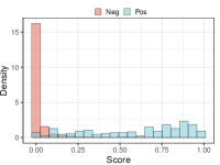
(a) Clean

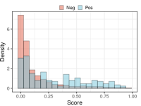
(b) FSGM

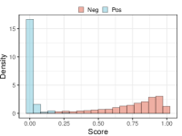
(c) PGD-10

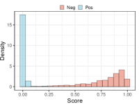
(d) PGD-20

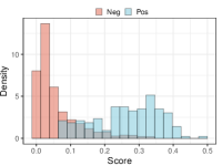
(e) Clean

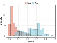
(f) FSGM

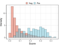
(g) PGD-10

(h) PGD-20

Figure 5: Distribution of positive and negative example scores of CE on MNIST-LT dataset. The first row represents the score distribution against different attacks under Natural Training, and the second row represents the score distribution under Adversarial Training.

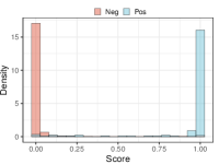
(a) Clean

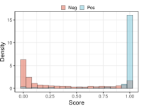
(b) FSGM

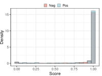
(c) PGD-10

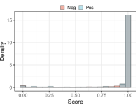
(d) PGD-20

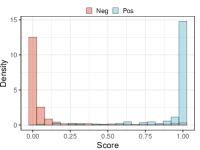
(e) Clean

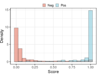
(f) FSGM

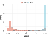
(g) PGD-10

(h) PGD-20

Figure 6: Distribution of positive and negative example scores of our proposed AdAUC on MNIST-LT dataset. The first row represents the score distribution against different attacks under Natural Training, and the second row represents the score distribution under Adversarial Training.

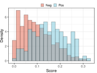
(a) Clean

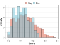
(b) FSGM

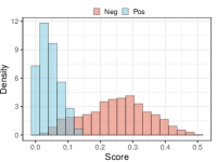
(c) PGD-10

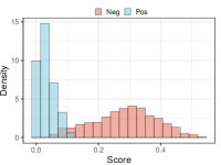
(d) PGD-20

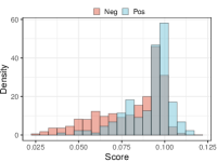
(e) Clean

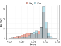
(f) FSGM

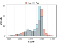
(g) PGD-10

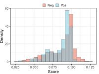
(h) PGD-20

Figure 7: Distribution of positive and negative example scores of CE on CIFAR-10-LT dataset. The first row represents the score distribution against different attacks under Natural Training, and the second row represents the score distribution under Adversarial Training.

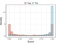
(a) Clean

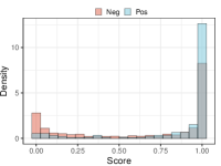
(b) FSGM

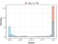
(c) PGD-10

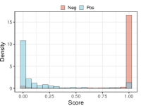
(d) PGD-20

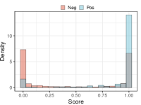
(e) Clean

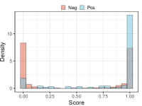
(f) FSGM

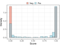
(g) PGD-10

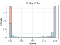
(h) PGD-20

Figure 8: Distribution of positive and negative example scores of AdAUC on CIFAR-10-LT dataset. The first row represents the score distribution against different attacks under Natural Training, and the second row represents the score distribution under Adversarial Training.

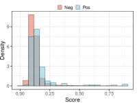
(a) Clean

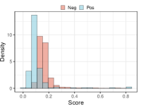
(b) FSGM

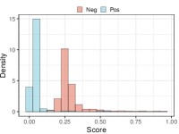
(c) PGD-10

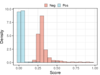
(d) PGD-20

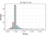
(e) Clean

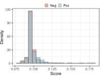
(f) FSGM

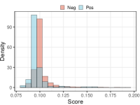
(g) PGD-10

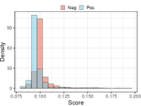
(h) PGD-20

Figure 9: Distribution of positive and negative example scores of CE on CIFAR-100-LT dataset. The first row represents the score distribution against different attacks under Natural Training, and the second row represents the score distribution under Adversarial Training.

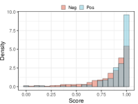
(a) Clean

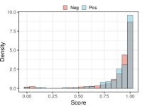
(b) FSGM

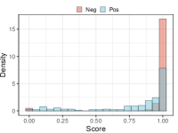
(c) PGD-10

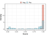
(d) PGD-20

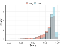
(e) Clean

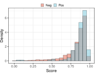
(f) FSGM

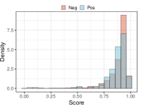
(g) PGD-10

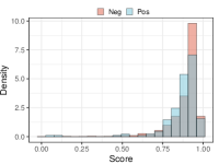
(h) PGD-20

Figure 10: Distribution of positive and negative example scores of AdAUC on CIFAR-100-LT dataset. The first row represents the score distribution against different attacks under Natural Training, and the second row represents the score distribution under Adversarial Training.

References

• Agarwal (2014) Agarwal, S. Surrogate regret bounds for bipartite ranking via strongly proper losses. The Journal of Machine Learning Research, 15(1):1653–1674, 2014.
• Agarwal et al. (2005) Agarwal, S., Graepel, T., Herbrich, R., Har-Peled, S., Roth, D., and Jordan, M. I. Generalization bounds for the area under the roc curve. Journal of Machine Learning Research, 6(4), 2005.
• Allen-Zhu et al. (2019) Allen-Zhu, Z., Li, Y., and Song, Z. A convergence theory for deep learning via over-parameterization. In International Conference on Machine Learning, pp. 242–252, 2019.
• Athalye & Carlini (2018) Athalye, A. and Carlini, N. On the robustness of the cvpr 2018 white-box adversarial example defenses. arXiv preprint arXiv:1804.03286, 2018.
• Athalye et al. (2018) Athalye, A., Carlini, N., and Wagner, D. Obfuscated gradients give a false sense of security: Circumventing defenses to adversarial examples. In International conference on machine learning, pp. 274–283. PMLR, 2018.
• Bai et al. (2022) Bai, Y., Gautam, T., and Sojoudi, S. Efficient global optimization of two-layer relu networks: Quadratic-time algorithms and adversarial training. CoRR, abs/2201.01965, 2022.
• Bao et al. (2020) Bao, H., Scott, C., and Sugiyama, M. Calibrated surrogate losses for adversarially robust classification. In Conference on Learning Theory, pp.  408–451. PMLR, 2020.
• Biggio et al. (2013) Biggio, B., Corona, I., Maiorca, D., Nelson, B., Šrndić, N., Laskov, P., Giacinto, G., and Roli, F. Evasion attacks against machine learning at test time. In Joint European Conference on Machine Learning and Knowledge Discovery in Databases, pp.  387–402, 2013.
• Böhm & Wright (2021) Böhm, A. and Wright, S. J. Variable smoothing for weakly convex composite functions. Journal of optimization theory and applications, 188(3):628–649, 2021.
• Cai et al. (2018) Cai, Q.-Z., Liu, C., and Song, D. Curriculum adversarial training. In Proceedings of the 27th International Joint Conference on Artificial Intelligence, pp.  3740–3747, 2018.
• Carlini & Wagner (2017) Carlini, N. and Wagner, D. Towards evaluating the robustness of neural networks. In IEEE Symposium on Security and Privacy, pp.  39–57, 2017.
• Clémençon et al. (2008) Clémençon, S., Lugosi, G., and Vayatis, N. Ranking and empirical minimization of u-statistics. The Annals of Statistics, 36(2):844–874, 2008.
• Cortes & Mohri (2003) Cortes, C. and Mohri, M. Auc optimization vs. error rate minimization. Advances in neural information processing systems, 16:313–320, 2003.
• Croce & Hein (2020) Croce, F. and Hein, M. Reliable evaluation of adversarial robustness with an ensemble of diverse parameter-free attacks. In International Conference on Machine Learning, pp. 2206–2216, 2020.
• Du et al. (2019) Du, S., Lee, J., Li, H., Wang, L., and Zhai, X. Gradient descent finds global minima of deep neural networks. In International Conference on Machine Learning, pp. 1675–1685, 2019.
• Fawcett (2006) Fawcett, T. An introduction to roc analysis. Pattern Recognition Letters, 27(8):861–874, 2006.
• Feizi (2020) Feizi, A. Hierarchical detection of abnormal behaviors in video surveillance through modeling normal behaviors based on auc maximization. Soft Computing, 24(14):10401–10413, 2020.
• Gao & Zhou (2015) Gao, W. and Zhou, Z.-H. On the consistency of auc pairwise optimization. In Twenty-Fourth International Joint Conference on Artificial Intelligence, 2015.
• Gao et al. (2013) Gao, W., Jin, R., Zhu, S., and Zhou, Z.-H. One-pass auc optimization. In International conference on machine learning, pp. 906–914, 2013.
• Gola et al. (2020) Gola, D., Erdmann, J., Müller-Myhsok, B., Schunkert, H., and König, I. R. Polygenic risk scores outperform machine learning methods in predicting coronary artery disease status. Genetic epidemiology, 44(2):125–138, 2020.
• Goodfellow et al. (2014) Goodfellow, I. J., Pouget-Abadie, J., Mirza, M., Xu, B., Warde-Farley, D., Ozair, S., Courville, A., and Bengio, Y. Generative adversarial nets. In Proceedings of the 27th International Conference on Neural Information Processing Systems, pp.  2672–2680, 2014.
• Goodfellow et al. (2015) Goodfellow, I. J., Shlens, J., and Szegedy, C. Explaining and harnessing adversarial examples. In International Conference on Learning Representations, 2015.
• Hand & Till (2001) Hand, D. J. and Till, R. J. A simple generalisation of the area under the roc curve for multiple class classification problems. Machine Learning, 45(2):171–186, 2001.
• Hanley & McNeil (1982) Hanley, J. A. and McNeil, B. J. The meaning and use of the area under a receiver operating characteristic (roc) curve. Radiology, 143(1):29–36, 1982.
• Herschtal & Raskutti (2004) Herschtal, A. and Raskutti, B. Optimising area under the roc curve using gradient descent. In Proceedings of the twenty-first international conference on Machine learning, pp.  49, 2004.
• Joachims (2005) Joachims, T. A support vector method for multivariate performance measures. In Proceedings of the 22nd international conference on Machine learning, pp.  377–384, 2005.
• Kurakin et al. (2017) Kurakin, A., Goodfellow, I., and Bengio, S. Adversarial machine learning at scale. In International Conference on Learning Representations, 2017.
• LeCun et al. (1998) LeCun, Y., Bottou, L., Bengio, Y., and Haffner, P. Gradient-based learning applied to document recognition. Proceedings of the IEEE, 86(11):2278–2324, 1998.
• Lin et al. (2020) Lin, T., Jin, C., and Jordan, M. On gradient descent ascent for nonconvex-concave minimax problems. In International Conference on Machine Learning, pp. 6083–6093, 2020.
• Liu et al. (2019) Liu, M., Yuan, Z., Ying, Y., and Yang, T. Stochastic auc maximization with deep neural networks. In International Conference on Learning Representations, 2019.
• Liu et al. (2021) Liu, M., Rafique, H., Lin, Q., and Yang, T. First-order convergence theory for weakly-convex-weakly-concave min-max problems. Journal of Machine Learning Research, 22(169):1–34, 2021.
• Madry et al. (2018) Madry, A., Makelov, A., Schmidt, L., Tsipras, D., and Vladu, A. Towards deep learning models resistant to adversarial attacks. In International Conference on Learning Representations, 2018.
• Maini et al. (2020) Maini, P., Wong, E., and Kolter, Z. Adversarial robustness against the union of multiple perturbation models. In International Conference on Machine Learning, pp. 6640–6650. PMLR, 2020.
• Natole et al. (2018) Natole, M., Ying, Y., and Lyu, S. Stochastic proximal algorithms for auc maximization. In International Conference on Machine Learning, pp. 3710–3719. PMLR, 2018.
• Nesterov (1998) Nesterov, Y. Introductory lectures on convex programming volume i: Basic course. Lecture notes, 3(4):5, 1998.
• Neumann (1928) Neumann, J. v. Zur theorie der gesellschaftsspiele. Mathematische Annalen, 100(1):295–320, 1928.
• Pang et al. (2019) Pang, T., Xu, K., Du, C., Chen, N., and Zhu, J. Improving adversarial robustness via promoting ensemble diversity. In International Conference on Machine Learning, pp. 4970–4979. PMLR, 2019.
• Ren et al. (2018) Ren, K., Yang, H., Zhao, Y., Chen, W., Xue, M., Miao, H., Huang, S., and Liu, J. A robust auc maximization framework with simultaneous outlier detection and feature selection for positive-unlabeled classification. IEEE transactions on neural networks and learning systems, 30(10):3072–3083, 2018.
• Robles et al. (2020) Robles, E., Zaidouni, F., Mavromoustaki, A., and Refael, P. Threshold optimization in multiple binary classifiers for extreme rare events using predicted positive data. In AAAI Spring Symposium: Combining Machine Learning with Knowledge Engineering (1), 2020.
• Shafahi et al. (2019) Shafahi, A., Najibi, M., Ghiasi, A., Xu, Z., Dickerson, J., Studer, C., Davis, L. S., Taylor, G., and Goldstein, T. Adversarial training for free! In Proceedings of the 33rd International Conference on Neural Information Processing Systems, pp.  3358–3369, 2019.
• Shafahi et al. (2020) Shafahi, A., Najibi, M., Xu, Z., Dickerson, J., Davis, L. S., and Goldstein, T. Universal adversarial training. In Proceedings of the AAAI Conference on Artificial Intelligence, pp.  5636–5643, 2020.
• Sinha et al. (2018) Sinha, A., Namkoong, H., and Duchi, J. Certifying some distributional robustness with principled adversarial training. In International Conference on Learning Representations, 2018.
• Sion (1958) Sion, M. On general minimax theorems. Pacific Journal of Mathematics, 8(1):171–176, 1958.
• Sorin et al. (2020) Sorin, V., Barash, Y., Konen, E., and Klang, E. Deep learning for natural language processing in radiology—fundamentals and a systematic review. Journal of the American College of Radiology, 17(5):639–648, 2020.
• Strubell et al. (2019) Strubell, E., Ganesh, A., and McCallum, A. Energy and policy considerations for deep learning in nlp. In Proceedings of the 57th Annual Meeting of the Association for Computational Linguistics, pp.  3645–3650, 2019.
• Szegedy et al. (2014) Szegedy, C., Zaremba, W., Sutskever, I., Bruna, J., Erhan, D., Goodfellow, I., and Fergus, R. Intriguing properties of neural networks. In International Conference on Learning Representations, 2014.
• Tramèr & Boneh (2019) Tramèr, F. and Boneh, D. Adversarial training and robustness for multiple perturbations. In Proceedings of the 33rd International Conference on Neural Information Processing Systems, pp.  5866–5876, 2019.
• Tramèr et al. (2017) Tramèr, F., Kurakin, A., Papernot, N., Boneh, D., and McDaniel, P. Ensemble adversarial training: Attacks and defenses. stat, 1050:30, 2017.
• Tu et al. (2019) Tu, Z., Zhang, J., and Tao, D. Theoretical analysis of adversarial learning: A minimax approach. In Wallach, H., Larochelle, H., Beygelzimer, A., d'Alché-Buc, F., Fox, E., and Garnett, R. (eds.), Advances in Neural Information Processing Systems, volume 32. Curran Associates, Inc., 2019.
• Usunier et al. (2005) Usunier, N., Amini, M.-R., and Gallinari, P. A data-dependent generalisation error bound for the auc. In Proceedings of the ICML 2005 Workshop on ROC Analysis in Machine Learning. Citeseer, 2005.
• Voulodimos et al. (2018) Voulodimos, A., Doulamis, N., Doulamis, A., and Protopapadakis, E. Deep learning for computer vision: A brief review. Computational intelligence and neuroscience, 2018, 2018.
• Wang et al. (2019a) Wang, Y., Ma, X., Bailey, J., Yi, J., Zhou, B., and Gu, Q. On the convergence and robustness of adversarial training. In International Conference on Machine Learning, pp. 6586–6595, 2019a.
• Wang et al. (2019b) Wang, Y., Zou, D., Yi, J., Bailey, J., Ma, X., and Gu, Q. Improving adversarial robustness requires revisiting misclassified examples. In International Conference on Learning Representations, 2019b.
• Westcott et al. (2019) Westcott, A., Capaldi, D. P., McCormack, D. G., Ward, A. D., Fenster, A., and Parraga, G. Chronic obstructive pulmonary disease: thoracic ct texture analysis and machine learning to predict pulmonary ventilation. Radiology, 293(3):676–684, 2019.
• Wong et al. (2019) Wong, E., Rice, L., and Kolter, J. Z. Fast is better than free: Revisiting adversarial training. In International Conference on Learning Representations, 2019.
• Xing et al. (2021) Xing, Y., Song, Q., and Cheng, G. On the generalization properties of adversarial training. In International Conference on Artificial Intelligence and Statistics, pp.  505–513, 2021.
• Ying et al. (2016) Ying, Y., Wen, L., and Lyu, S. Stochastic online auc maximization. Advances in Neural Information Processing Systems, 29:451–459, 2016.
• Zagoruyko & Komodakis (2016) Zagoruyko, S. and Komodakis, N. Wide residual networks. In British Machine Vision Conference, 2016.
• Zhang et al. (2019a) Zhang, D., Zhang, T., Lu, Y., Zhu, Z., and Dong, B. You only propagate once: Accelerating adversarial training via maximal principle. Advances in Neural Information Processing Systems, 32:227–238, 2019a.
• Zhang et al. (2019b) Zhang, H., Yu, Y., Jiao, J., Xing, E., El Ghaoui, L., and Jordan, M. Theoretically principled trade-off between robustness and accuracy. In International Conference on Machine Learning, pp. 7472–7482. PMLR, 2019b.
• Zhang et al. (2020) Zhang, J., Zhu, J., Niu, G., Han, B., Sugiyama, M., and Kankanhalli, M. Geometry-aware instance-reweighted adversarial training. In International Conference on Learning Representations, 2020.
• Zhao et al. (2011) Zhao, P., Hoi, S. C., Jin, R., and Yang, T. Online auc maximization. In Proceedings of the 28th International Conference on International Conference on Machine Learning, pp.  233–240, 2011.