Construction of weaving and polycatenane
motifs from periodic tilings of the plane

Abstract.

Doubly periodic weaves and polycatenanes embedded in the thickened Euclidean plane are three-dimensional complex entangled structures whose topological properties can be encoded in any generating cell of its infinite planar representation. Such a periodic cell, called motif, is a specific type of link diagram embedded on a torus consisting of essential simple closed curves for weaves, or null-homotopic for polycatenanes. In this paper, we introduce a methodology to construct such motifs using the concept of polygonal link transformations. This approach generalizes to the Euclidean plane existing methods to construct polyhedral links in the three-dimensional space. Then, we will state our main result which allows one to predict the type of motif that can be built from a given planar periodic tiling and a chosen polygonal link method.

1. Introduction

Doubly periodic weaves and polycatenanes are complex three-dimensional entangled structures made of non-intersecting curves, which are open intertwined threads or closed linked rings, respectively. They are fascinating topological objects whose mathematical properties are also very useful for applications in materials science [9, 10, 11, 17, 21, 25, 27, 29]. In our previous work [13], we introduced a novel topological definition of particular classes of weaves, called untwisted and twisted weaves, as the projection to the Euclidean thickened plane of a quadrivalent planar graph consisting of infinite simple open curves with a crossing information at each vertex. In chemistry, polycatenanes are described as multiple linked rings [21, 30]. The Hopf link, which is the simplest pair of linked rings, is a classical catenane. More precisely, polycatenanes are characterized by the presence of more than two linked rings. In [30], a catenane is more generally defined as a disjoint union of knots. Here, we adopt the specific definition of a polycatenane as a disjoint union of trivial knots. As in knot theory, we are interested in studying the topological properties of these complex three-dimensional entangled objects at their planar diagrammatic scale [6, 7]. Recall that a link diagram is the natural projection of a link embedded in a general position in the three-dimensional to the Euclidean plane [24]. In the case of a doubly periodic diagram, it is more relevant to study a generating cell, as done by Grishanov, H. Morton et al. in [14, 23], as well as A. Kawauchi in [19]. It indeed appears that any periodic cell of a doubly periodic diagram is a particular type of link diagram on a torus, called a motif. In particular, we noticed that all the closed curve components are essential in the case of a weaving motif and null-homotopic for a polycatenane motif. We call a motif containing both essential and null-homotopic components is a mixed motif.

The first main purpose of this paper is to construct weaving and polycatenane motifs. Our strategy is to formalize and generalize to the case of periodic planar tilings [15], the methods to construct polyhedral links defined by W.Y. Qiu et al. in [16, 22, 26]. Their methods consist in transforming a polyhedron into a link by covering each edge with a single or double line, possibly with twists, and each vertex with a set of branched curves or crossed curves. When applied to the plane, we call these three methods polygonal link methods. The transformation of a periodic tiling into a weaving diagram by assigning an over or under information to each vertex has also been considered in [2, 3]. Note that we will not discuss the properties of crossings in this paper, and will construct alternating motifs by convention as explained in Section 2. We can introduce our notations in the following definition, where each case is detailed in Section 3.1, to describe the transformation of the vertices and edges of a given tiling periodic cell $\mathcal{T}$, called a $\mathcal{T}$-cell.

Definition 1.1.

A $\mathcal{T}$-cell is said to be transformed by the polygonal link method $(\Lambda,L)$, $L\in\{s,m\}$ with $m$ being a positive integer, and $\Lambda\in\{\mathit{C}_{r},\mathit{B}_{r}\}$, if all its vertices and all its edges are transformed by the same method with,

$$(\Lambda,L)=\left\{\begin{array}[]{lll}(\mathit{C}_{r},s)&\mbox{: crossed curves and single line covering},\\ (\mathit{C}_{r},m)&\mbox{: crossed curves and m-twisted double line covering},\\ (\mathit{B}_{r},m)&\mbox{: branched curves and m-twisted double line covering}.\\ \end{array}\right.$$

This generalization of the strategy of Qiu et al. to general planar graphs describes a systematic way to construct diagrams of entangled structures. Using a graph-theoretic approach to study the properties of knots and links has shown to be useful in many cases, such as in [4, 5, 8, 18, 20]. In the case of doubly periodic structures, we are interested in predicting whether a chosen method $(\Lambda,L)$ applied to a given $\mathcal{T}$-cell will create a weaving motif, a polycatenane motif or a mixed motif. Indeed, we noticed that each curve component generated by $(\Lambda,L)$ will cover a closed path, called a characteristic loop and denoted by $\Delta_{(\Lambda,L)}$, in the original skeleton of the $\mathcal{T}$-cell, as described in Section 3.2. Therefore, by using algebraic and combinatorial arguments, the second objective of this paper is to characterize such characteristic loops in the given $\mathcal{T}$-cell in order to predict the type of structure that will be construct. We will detail our following main result in Section 3.3, which can have interesting applications in other disciplines considering a computational approach.

Theorem 1.2.

(Motif Prediction Theorem)

Let $P$ be a $\mathcal{T}$-cell and $(\Lambda,L)$ be a polygonal link method. Then, $\big{(}P,(\Lambda,L)\big{)}$ generates

1. a weaving motif if and only if all the characteristic loops $\Delta_{(\Lambda,L)}$ in $P$ are essential, with at least two of them being non-parallel, and such that each of them has a word that can be written as a product of simple words,

2. a polycatenane motif if and only if each characteristic loops $\Delta_{(\Lambda,L)}$ in $P$ is null-homotopic and can be written as trivial word or as a product of simple words,

3. a mixed motif if and only if the set of all the characteristic loops $\Delta_{(\Lambda,L)}$ in $P$ contains at least an essential and a null-homotopic characteristic loops whose words can be written as trivial words and as a product of simple words.

In Section 2, we will recall and extend the main definitions of weaves, polycatenanes and their diagrams. In Section 3, we will state a formal definition of the polygonal link construction methods, and then prove our main theorem.

2. Preliminaries on weaves and polycatenanes

2.1. Weaves

We start this section by recalling the main definitions of weaves and their diagrams, stated in our previous work [13]. First, consider $N\geq 2$ infinite sets of straight lines embedded in the Euclidean plane $\mathbb{E}^{2}$, called color groups. Two such lines are said to be in the same color group if they do not intersect each other, namely if they are parallel, or in different color groups if they intersect once (Fig. 1(A)). Then, each intersection is specified by an over or under information (Fig. 1(B)), called crossing as in knot theory, which is encoded into a set of crossing sequences. A crossing sequence is a sequence of integers with minimal length describing the number of consecutive over or undercrossings of a given colored line with the element of a different color group. We refer to [13] for a more specific definition of crossing sequences. An untwisted weave (Fig. 1(C)) is then defined as the projection to the Euclidean thickened plane $\mathbb{X}^{3}=\mathbb{E}^{2}\times\mathrm{I}$, where $\mathrm{I}=[-1,1]$, of a pair consisting of a quadrivalent graph made of these colored straight lines, together with a crossing information to each vertex, under the natural projection map $\pi:\mathbb{X}^{3}\to\mathbb{E}^{2}$, $(x,y,z)\mapsto(x,y,0)$.

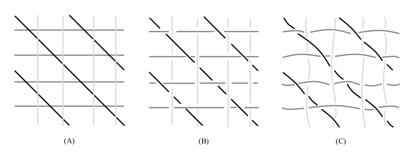
Figure 1. (A) Set of straight lines belonging to different color groups on the Euclidean plane. (B) Crossing information to each intersection on the Euclidean plane. (C) Untwisted weave in the thickened Euclidean plane.

Definition 2.1.

Let $N\geq 2$ be a positive integer and for all $i\in\{1,\cdots,N\}$, let $\Gamma_{i}$ be an infinite set of parallel straight lines of color $i$ embedded on $\mathbb{E}^{2}$. If $\Gamma=(\Gamma_{1},\cdots,\Gamma_{N})$ is a quadrivalent connected graph with a crossing information at each vertex encoded in a set of crossing sequences $\Sigma=\{\Sigma_{i,j}\}_{1\leq i<j\leq N}$, then we call untwisted weave the projection to $\mathbb{X}^{3}$ of the pair $(\Gamma,\Sigma)$ under the projection map $\pi$, which is an embedding of non-intersecting infinite curves in $\mathbb{X}^{3}$. Each projected line is called a thread and two threads are said to be in the same set of threads $T_{i}$ if they are the projection of straight lines belonging to the same color group $\Gamma_{i}$.

Next, consider that before mapping such a given pair $(\Gamma,\Sigma)$ (Fig. 2(A)) to the three-dimensional space, we operate a local surgery, called twists (Fig. 2(B)), which consists in introducing new crossings between two closest neighboring lines of a same color group, namely two closest parallel lines (Fig. 2(C)). This local twisting operation can be defined as a $\pm k$-move [1], as details in our previous work [13], and any topological disk containing only twists is called a twisted region. We can therefore define a twisted weave as the projection a pair $(\Gamma,\Sigma)$ containing at least one twisted region.

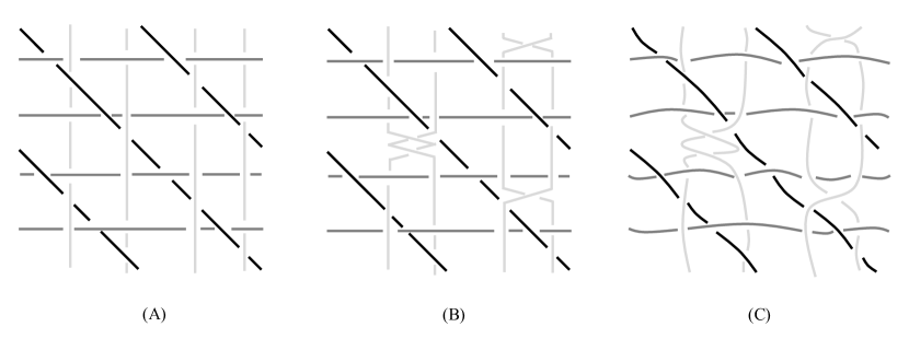
Figure 2. (A) Set of straight lines with crossing information on the Euclidean plane. (B) Introduction of twists on the Euclidean plane. (C) Twisted weave in the thickened Euclidean plane.

Definition 2.2.

A twisted weave is the projection to $\mathbb{X}^{3}$ of a pair $(\Gamma,\Sigma)$ satisfying Definition 2.1 admitting at least a twisted region. Moreover, if two threads twist their total number of twists is even and they cannot twist with any other threads.

2.2. Polycatenanes

In the introduction, we have seen that polycatenanes are described as multiple linked rings [21, 30]. In the language of knot theory, since such a ring can be intuitively seen as an unknot, we can formally defined a polycatenane as a link whose components are all isotopic to trivial knots. A Hopf link is a simple example of a polycatenane. More specifically, in our context of entangled structures embedded in a thickened plane, we suggest a similar topological definition as weaves with closed curve components instead. Let $\Xi=\{R_{1},R_{2},\cdots\}$ be an infinite set of simple closed curves embedded on $\mathbb{E}^{2}$, intersecting each other in double point only, but not themselves (Fig. 3(A)). In this case, note that the notion of color group is not considered since the rings do not need to be organized in different sets. Assign to each pair of such loops $R_{i}$ and $R_{j}$ a crossing sequence $C_{i,j}$, where $i$ and $j$ are distinct positive integers, and specify each vertex with an over or under information accordingly (Fig. 3(B)). The definition of a crossing sequence is similar as for weaves, meaning a sequence of integers with minimal length describing the number of consecutive over or undercrossings of a given ring $R_{i}$ with a distinct ring $R_{j}$.

Definition 2.3.

Let $i,j,k,l$ be positive integers, and let $R_{i}$ and $R_{j}$ be two distinct oriented simple closed curves of $\Xi=\{R_{1},R_{2},\cdots\}$ on $\mathbb{E}^{2}$, intersecting exactly $k$ times. Then by walking on $R_{i}$, the crossing sequence $C_{i,j}$ of $R_{i}$ with $R_{j}$ is defined either by,

1. a sequence $(+1,0)$ (resp. $(0,-1)$) if all the $k$ intersections are assigned an over (resp. under) information for $R_{i}$.

2. a finite sequence $(+p_{1},-p_{2},\cdots,+p_{l-1},-p_{l})$ of minimal length, where $p_{1},\cdots,p_{l}$ are strictly positive integers, such that there exists a crossing $c$ between $R_{i}$ and $R_{j}$ whose closest neighboring crossing in the opposite direction is an undercrossing, and from which $R_{i}$ will have $p_{1}$ consecutive overcrossings with $R_{j}$, followed by $p_{2}$ consecutive undercrossings, followed by $p_{3}$ consecutive overercrossings and so forth.

Moreover, we denote by $\Sigma=(C_{i,j})_{i<j}$, with $i,j$ distinct, the set of crossing sequences associated to the pair $(R_{i},R_{j})$.

Remark 2.4.

The crossing sequence $C_{j,i}$ is naturally deduced from $C_{i,j}$ for any pair $(R_{i},R_{j})$, and conversely. Recall that from the next section of this paper, we will restrict ourselves to the case of $C_{i,j}=(+1,-1)$ for all $i$ and $j$ distinct.

As for weaves, a polycatenane (Fig. 3(C)) can be defined as the projection to the thickened Euclidean plane of such a quadrivalent graph, with respect to a set of crossing sequences.

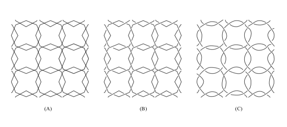
Figure 3. (A) Sets of intersecting simple closed curves in the Euclidean plane. (B) Crossing information to each intersection in the Euclidean plane. (C) Polycatenane in the thickened Euclidean plane view from the top.

Definition 2.5.

Let $\Xi=\{R_{1},R_{2},\cdots\}$ be a set of infinitely many simple closed curves embedded on $\mathbb{E}^{2}$, with a crossing information at each vertex given by a set of crossing sequences $\Sigma=(C_{i,j})_{i<j}$, with $i,j$ distinct positive integers. Then, we call polycatenane the projection to $\mathbb{X}^{3}$ under the map $\pi$ of the pair $(\Xi,\Sigma)$, which is an embedding of non-intersecting simple closed curves in $\mathbb{X}^{3}$, called rings.

2.3. Diagrammatic representation and motifs

A weave or a polycatenane in a general position in $\mathbb{X}^{3}$ can be projected onto the Euclidean plane by the map $\pi$, as in knot theory [24]. By general position, we mean that the planar projection of two components, threads or rings, by the natural projection map $\pi$ are distinct. This projection leads to a planar quadrivalent connected graph with crossing information, meaning that all the vertices have degree four and are assigned an over or under information. Moreover, if this planar structure is doubly periodic, then any periodic cell defines a particular link diagram on a torus, as seen in [14]. From now, we will use the terms entangled structures to enclose weaves, polycatenanes and mixed structures.

Definition 2.6.

The projection of an entangled structure onto $\mathbb{X}^{2}$ by the map $\pi:\mathbb{X}^{3}\to\mathbb{E}^{2}$, $(x,y,z)\mapsto(x,y,0)$ is called a regular projection. If each vertex is specified by an over or under information, then this projection is called an infinite diagram.

An entangled diagram $D$ admitting translation symmetry on two non-parallel directions in $\mathbb{E}^{2}$ is said to be doubly periodic. This implies the existence of a discrete group $G$ generated by two independent translations, called periodic lattice such that the quotient of $(D,\mathbb{E}^{2})$ by $G$ is a periodic cell $U$ of $D$.

Definition 2.7.

Let $D$ be a doubly periodic entangled diagram on $\mathbb{E}^{2}$ with periodic lattice $G$. Then, a periodic unit cell $U$ of $D$ for $G$, defined as the quotient of $D$ by $G$, is a link diagram on a torus $T^{2}$ called a motif.

By reducing the study of doubly periodic entangled structures to their unit cells, we are able to classify them from a knot theoretical point of view, with additional considerations that encode the periodicity. A motif is defined as a set a closed curves on a torus intersecting each other, and possibly themselves, in transverse double points specified by a crossing information. To characterize the relation between such a link diagram on a torus and the corresponding doubly periodic entangled diagram on the universal cover, we must recall some classic definitions from algebraic topology [12].

Let $T^{2}$ be a torus defined as the quotient space of the Euclidean plane $\mathbb{E}^{2}$ by a periodic lattice $G$ isomorphic to $\mathbb{Z}^{2}$. Then, a closed curve $\omega$ in $T^{2}$ is a continuous map

$$\omega:S^{1}\mapsto T^{2}.$$

Any such closed curve $\omega_{1}$ on $T^{2}$ can be continuously deformed into another curve $\omega_{2}$ by a map $h:S^{1}\times[0,1]\mapsto T^{2}$ where $h(x,0)=\omega_{1}(x)$ and $h(x,1)=\omega_{2}(x)$. In this case, $\omega_{1}$ and $\omega_{2}$ are said to be homotopic, which states a notion of equivalence between the two curves.

There exists two types of closed curves on a torus, namely essential closed curves and contractible ones. A contractible curve, also called null-homotopic, is defined to be homotopic to a constant curve, which intuitively means that it can be continuously contracted to a single point. Otherwise, the curve is essential.

Then, a curve is said to be simple if it does not admit any self-intersection, or in other words if the map $\omega$ is injective. Conversely, a non-simple curve admits a finite number of self-intersections, each being a transverse double point, such that $\omega$ is injective everywhere except at those singular points.

We are interesting in characterizing the images of each of these different curves on $\mathbb{E}^{2}$, as being the covering space of $T^{2}$ by the continuous map

$$\lambda:\mathbb{E}^{2} \to T^{2}$$

$$\mathbb{R} \mapsto S^{1}$$

The image $\omega\circ\lambda$ of a closed curve $\omega$ in $T^{2}$ to $\mathbb{E}^{2}$ by the map $\lambda$ is called a lift of the curve $\omega$. If $\omega$ is essential on $T^{2}$, then it lifts to a set of infinite parallel open curves in $\mathbb{E}^{2}$, where two such curves are said to be parallel since they run along the same axis of direction. In other words, if the lift of an essential closed curve $\omega_{1}$ by $p$ is a translate to another curve $\omega_{2}$, then $\lambda\circ\omega_{1}=\lambda\circ\omega_{2}$ and $\omega_{1}$ and $\omega_{2}$ are also said to be parallel on $T^{2}$.

Finally, note that the lift of a self-intersecting curve $\omega$ on $T^{2}$ may or may not self-intersect on $\mathbb{E}^{2}$, which is an important point to consider here since weaving, polycatenane and mixed infinite diagrams consist only of curves without self-intersections. We refer to [28] for the details of the following arguments.

Definition 2.8.

Let $p$ be a self-intersection point of $\omega$. Then, $p$ divides $\omega$ into two closed curves, both being seen as homology cycles. By walking on these loops starting from $p$, one will return to $p$ from the left of the starting direction and the other from the right, both being denoted by $\omega_{p}$ and $\omega^{\prime}p$, respectively. We call $\omega_{p}$ and $\omega^{\prime}_{p}$ the divided curves of $\omega$ for $p$.

Next, we define the quotient $T^{2}=\mathbb{E}^{2}\setminus\mathbb{Z}^{2}$, as well as the restriction

$$\Omega:[0,1]\mapsto\mathbb{E}^{2}$$

of the lift $\omega\circ\lambda$ to $\mathbb{E}^{2}$, such that $\Omega(0)=(0,0)$. First, consider the case where $\omega$ is an essential curve on $T^{2}$. Then, $\omega\neq 0$ in the first homology group of the torus $H_{1}(T^{2},\mathbb{Z})$, which defines the equivalence classes of cycles. Thus, $\Omega(1)\neq\Omega(0)$. If $\omega_{p}\neq 0$ and $\omega^{\prime}_{p}\neq 0$ in homology, then the intersection point $p$ vanishes on the lift $\Omega$. Otherwise, if $\omega_{p}=0$ or $\omega^{\prime}_{p}=0$ in homology, then the lift of such a trivial divided curve is a closed component on $\mathbb{E}^{2}$ since $H_{1}(T^{2},\mathbb{Z})$ is isomorphic to the fundamental group of the torus with basepoint $p$, and thus the intersection point is also lifted. Similarly, if $\omega$ is a null-homotopic self-intersecting curve.

Therefore, by definition of a motif as a generating cell of a doubly periodic diagram, the characterization of each type of entangled structure as a link diagram on a torus follows by identification of opposite sides of a unit cell [14].

Definition 2.9.

(Link diagram of a doubly periodic entangled structure)

Let $D$ be a doubly periodic entangled diagram on $\mathbb{E}^{2}$ with periodic lattice $G$ and let $U$ be a corresponding motif.

• A weaving motif is a link diagram consisting of at least two non-parallel essential closed curves without trivial divided curves.

• A polycatenane motif is a link diagram whose components are null-homotopic closed curves without trivial divided curves.

Moreover, we call mixed motif a link diagram containing both types of components.

Note that the case of a link diagram with only parallel essential curve components is not cover in this paper. We conclude this section by recalling the notion of equivalence adopted for doubly periodic entangled structures, as defined by S. Grishanov et al. in [14], generalizing the classical Reidemeister Theorem to periodic torus diagrams.

Definition 2.10.

Two entangled structures in $\mathbb{X}^{3}$ are said to be equivalent if their infinite diagrams can be obtained from each other by a sequence of Reidemeister moves $R_{1}$, $R_{2}$, $R_{3}$ and planar isotopies. Moreover, for doubly periodic structures, equivalent motifs are invariant under torus isotopies and torus twists.

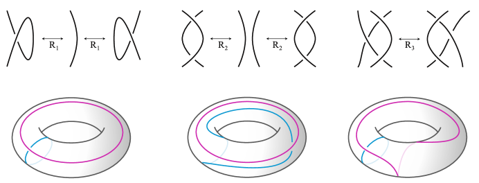
Figure 4. On the top, the three classical Reidemeister moves. On the bottom, a torus with a meridian and a longitude curves (left), its longitudinal twist (middle) and its meridional twist (right)

Note that in the case of a doubly periodic weave, definitions of untwisted and twisted weaves are naturally reduced to a thickened parallelogram unit cell with boundary conditions, that is copied by translation in two non-parallel directions. In particular, the twisting surgery appears in such a generating cell, which obviously implied that a doubly periodic twisted weave contains infinitely many twists.

3. Weaving and polycatenane motifs constructed by polygonal links

In this section, we first give a formal mathematical description of the polygonal link methods, which were originally introduced by W.Y. Qiu et al. in [16, 22, 26] to transform polyhedra into links. Then, using algebraic and combinatorial arguments, we will define a strategy to predict the type of entangled structure a given polygonal link method applied to a chosen periodic tiling of the plane can create, namely a weaving motif, a polycatenane motif or a mixed motif. Recall that on a torus, the components of a weaving motif are essential closed curves, a polycatenane motif contains only null-homotopic closed curves, and the set of components of a mixed motif contains at least one of each.

3.1. Polygonal link methods

From the definitions stated in the previous section, we have seen that an entangled diagram can be constructed by assigning an over or under information to each vertex of a particular type of quadrivalent graph. As mentioned above, we will not discuss the properties of crossings in this paper and we will consider that all the diagram are alternating by convention. An entangled structure is to be alternating if its crossings alternate cyclically between undercrossings and overcrossings, as one travels along each of its components. In [16, 22, 26], new methods to transform a polyhedron into a polyhedral link are introduced, which consist in transforming each edge and each vertex by one of the methods illustrated in Fig. 5. We generalize these transformations to planar graphs and name them polygonal link methods.

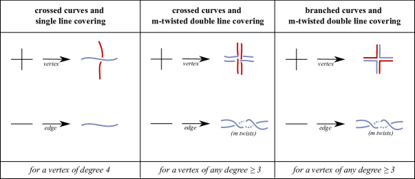
Figure 5. Polygonal link methods: transformation of a vertex and its adjacent edges.

Let $P$ be any generating cell of a given doubly periodic topological polygonal tessellation of $\mathbb{E}^{2}$. Then, our strategy is to obtain a systematic way to construct entangled motifs by transforming simultaneously all the vertices and edges of $P$ using the same polygonal link method. By a polygonal tessellation is meant a covering of the plane by polygons, called tiles, such that the interior points of the tiles are pairwise disjoint. We restrict to tilings which are also edge-to-edge, meaning that the vertices are corners of all the incident polygons. However, we do not consider geometric constrains such as lengths and angles, meaning that tilings by squares or parallelograms are considered equivalent here, for example. More specifically, two polygonal tessellations are said to be topologically equivalent if one can be mapped to the other by a homeomorphism preserving the degree of the vertices and the number of adjacent neighbors of each tile, as defined in [15]. We will call any doubly periodic tiling $\mathcal{T}$ satisfying all these conditions a 2-tiling for simpler notation and any generating cell a $\mathcal{T}$-cell. We start by introducing a formal definition of the methods illustrated in Fig. 5, considering a right-handed orientation of the plane from now on.

Definition 3.1.

Let $e_{v,v^{\prime}}$ be the edge of a given $\mathcal{T}$-cell connecting the vertices $v$ and $v^{\prime}$. Then $e_{v,v^{\prime}}$ is said to be transformed by,

• a single line covering, if it is replaced by a single strand $s_{v,v^{\prime}}$;

• an $m$-twisted double line covering, if it is replaced by a pair of strands $s_{v,v^{\prime}}$ and $s^{\prime}_{v,v^{\prime}}$ crossing $m$ times in an alternating fashion, with $m$ a positive integer.

Remark 3.2.

In the case of an $m$-twisted double line covering, we will decompose the strands into three connected segments,

$$s_{v,v^{\prime}}=s_{v_{r},v^{\prime}}\cup S_{v,v^{\prime}}\cup s_{v,v^{\prime}_{\mu}},$$

$$s^{\prime}_{v,v^{\prime}}=s^{\prime}_{v_{l},v^{\prime}}\cup S^{\prime}_{v,v^{\prime}}\cup s^{\prime}_{v,v^{\prime}_{\mu}},$$

with $\mu\in\{l,r\}$, where $l$ stand for left and $r$ for right. To assign the value $\mu$, consider a neighboring disk $D_{v}$ of the vertex $v$ and orient the edge $e_{v,v^{\prime}}$ toward $v$ in $D_{v}$. This implies that in a neighboring disk $D_{v^{\prime}}$ of the vertex $v^{\prime}$, the orientation of $e_{v,v^{\prime}}$ is opposite since it is now toward $v^{\prime}$. Each such edge segment separates its neighborhoods into a left and a right regions, with respect to its orientation. Therefore, if an edge is covered by an $m$-twisted double line, then in the interior of those disks, one of the strand is said to be on the left and the other on the right (Fig. 6). We denote by $S_{v,v^{\prime}}$ (resp. $S^{\prime}_{v,v^{\prime}}$) the curves that connect the strand on the right (resp. left) in $D_{v}$ with one of the strand in $D_{v^{\prime}}$. We will use the following convention.

• If $m=0$ or $m$ is even,

  $$s_{v,v^{\prime}}=s_{v_{r},v^{\prime}}\cup S_{v,v^{\prime}}\cup s_{v,v^{\prime}_{l}},$$

  $$s^{\prime}_{v,v^{\prime}}=s_{v_{l},v^{\prime}}\cup S^{\prime}_{v,v^{\prime}}\cup s_{v,v^{\prime}_{r}}.$$

• If $m$ is odd,

  $$s_{v,v^{\prime}}=s_{v_{r},v^{\prime}}\cup S_{v,v^{\prime}}\cup s_{v,v^{\prime}_{r}},$$

  $$s^{\prime}_{v,v^{\prime}}=s_{v_{l},v^{\prime}}\cup S^{\prime}_{v,v^{\prime}}\cup s_{v,v^{\prime}_{l}}.$$

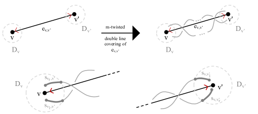
Figure 6. Strand labeling for an $m$-twisted double line covering.

Next, each vertex $v$ of degree $n\geq 3$ belonging to the given $\mathcal{T}$-cell will be transformed into an entangled area in three ways. At the neighborhood $D_{v}$ of $v$, we label its adjacent edge segments starting from an arbitrary edge $e_{v}=(e_{v})_{0}$. Then, its first counterclockwise adjacent edge is $(e_{v})_{1}$, the second adjacent edge is $(e_{v})_{2}$, and so forth such that $(e_{v})_{0}=(e_{v})_{n}$. Conversely, by reading clockwise, its first adjacent edge is $(e_{v})_{-1}$, the second adjacent edge is $(e_{v})_{-2}$, and so forth such that $(e_{v})_{0}=(e_{v})_{-n}$ (see Fig. 7).

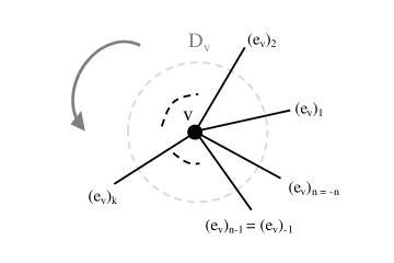
Figure 7. Edge labeling at a neighborhood of a vertex $v$ of degree $n$.

For a single line covering transformation at the edges, the only option for the adjacent vertex is a crossed curves transformation, and is only allowed if the degree of the vertex is four. In that case, each pair of opposite strands are glued into a single strand, and we will use the convention that at the construction time, the strand being the union of $(s_{v})_{1}$ and $(s_{v})_{3}$ will be over the second strand, where a strand $(s_{v})_{i}$ replaced the edge segment $(e_{v})_{i}$ in $D_{v}$, for $i=0,1,2,3$. Such a crossing information can be reverse. However, for an $m$-twisted double line covering transformation at the edges, there are two options. One possibility is to connect each right strand $(s_{v_{r},v^{\prime}})_{i}$ in $D_{v}$ to its closest neighboring left strand $(s_{v_{l},v^{\prime\prime}})_{i+1}$, constructed from the edge adjacent to the vertices $v$ and $v^{\prime\prime}\neq v^{\prime}$, by a branched curves transformation. Otherwise, a crossed curves transformation is also possible in this case by connected each right strand $(s_{v_{r},v^{\prime}})_{i}$ to the second counterclockwise adjacent left strand $(s_{v_{l},v^{\prime\prime}})_{i+2}$. For these two transformations, we will use the convention that at the resulting crossings, the left strand is always over, and the right strand under, with the possibility to reverse the crossing information afterwards.

Definition 3.3.

Each vertex $v$ of degree $n_{v}\geq 3$ of a $\mathcal{T}$-cell is said to be transformed by,

• crossed curves, if $n_{v}=4$ and if each strand $(s_{v,v^{\prime}})_{i}$ is glued to the strand $(s_{v,v^{\prime\prime}})_{i+2}$ to become a single strand, where each edge adjacent to $v$ has been replaced by a single line covering, and $v,v^{\prime},v^{\prime\prime}$ are distinct adjacent vertices;

• crossed curves, meaning that each strand $(s_{v_{r},v^{\prime}})_{i}$ connects with the strand $(s_{v_{l},v^{\prime\prime}})_{i+2}$ to become a single strand, where each edge adjacent to $v$ has been replaced by an $m$-twisted double line covering, $m\geq 0$, and $v,v^{\prime},v^{\prime\prime}$ are distinct adjacent vertices;

• branched curves, meaning that each strand $(s_{v_{r},v^{\prime}})_{i}$ connects with the strand $(s_{v_{l},v^{\prime\prime}})_{i+1}$ to become a single strand, where each edge adjacent to $v$ has been replaced by an $m$-twisted double line covering, $m\geq 0$, and $v,v^{\prime},v^{\prime\prime}$ are distinct adjacent vertices.

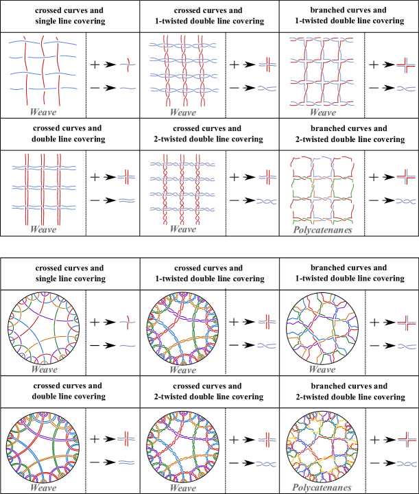
Figure 8. Examples of weave and polycatenane diagrams constructed from a periodic Euclidean tiling (top) and hyperbolic tiling (bottom).

We can summarize the transformation of the vertices and edges of a given $\mathcal{T}$-cell by one of the three different methods in the following definition, illustrated in Fig. 8.

Definition 3.4.

A $\mathcal{T}$-cell is said to be transformed by the polygonal link method $(\Lambda,L)$, $L\in\{s,m\}$, $m$ being a positive integer, and $\Lambda\in\{\mathit{C}_{r},\mathit{B}_{r}\}$, if all its vertices and all its edges are transformed by the same method with,

$$(\Lambda,L)=\left\{\begin{array}[]{lll}(\mathit{C}_{r},s)&\mbox{: crossed curves and single line covering},\\ (\mathit{C}_{r},m)&\mbox{: crossed curves and $m$-twisted double line covering},\\ (\mathit{B}_{r},m)&\mbox{: branched curves and $m$-twisted double line covering}.\\ \end{array}\right.$$

Remark 3.5.

In this paper, we discussed the transformation of doubly periodic tilings of the Euclidean plane. However, we can also apply the same polygonal link methods to hyperbolic periodic tilings to construct hyperbolic motifs and diagrams, see Fig. 8. Moreover, such transformations can also be applied to non-periodic planar tilings or graphs.

3.2. Characteristic loops of polygonal link methods

The second main purpose of this paper is to predict whether a $(\Lambda,L)$ method applied to a chosen $\mathcal{T}$-cell will generate a weaving motif, a polycatenane motif or a mixed motif. We indeed observed cases where closed curve components were created in the universal cover which motivated this study, such as the polycatenane in Fig. 8. However, this provides the opportunity to characterize different types of entangled doubly periodic objects. Given a $\mathcal{T}$-cell with labelled and oriented edges, our strategy is to predict the type of polygonal chains that will be covered by the curve components created from the chosen $(\Lambda,L)$ method. Such a polygonal chain is homotopic to a closed curve on a torus by definition, and is therefore either null-homotopic or essential by periodic conditions as seen above. We call such a closed path a characteristic loop of $(\Lambda,L)$ and characterize it combinatorially.

Definition 3.6.

Let $P$ be an arbitrary $\mathcal{T}$-cell and $(\Lambda,L)$ a given polygonal link method. A characteristic loop of $(\Lambda,L)$ is an oriented closed curve homotopic to a polygonal chain in $P$ defined by an ordered and reduced iterative sequence of adjacent oriented edges,

$$\Delta_{(\Lambda,L)}=(\delta_{0}^{\pm},\delta_{1}^{\pm},\cdots,\delta_{k}^{\pm})_{(\Lambda,L)},$$ (3.1)

where $\delta_{k}^{+}$ and $\delta_{k}^{-}$ denote the same edge with opposite orientation, and $\delta_{0}$ and $\delta_{k}$ being edges of $P$ sharing a common vertex, with $k$ a positive integer.

We define such a closed polygonal chain for the three distinct $(\Lambda,L)$ methods independently, see Fig. 9 and Fig. 10 for two examples on a triangular tiling.

3.2.1. Crossed curves and single line covering: $(\Lambda,L)=(\mathit{C}_{r},s)$

Lemma 3.7.

If $(\Lambda,L)=(\mathit{C}_{r},s)$, then for all $i\in(1,...,k)$ a characteristic loop,

$$\Delta_{(C_{r},s)}=(\delta_{0}^{\pm},\delta_{1}^{\pm},\cdots,\delta_{k}^{\pm})_{(C_{r},s)},$$

is defined by the iterative sequence,

$$\delta_{i}=(\delta_{i-1})_{2}\mbox{ and }\delta_{0}=(\delta_{k})_{2},$$ (3.2)

where each $\delta_{i}$ is an edge of $P$ covered by a single line.

Proof.

Let $P$ be an arbitrary $\mathcal{T}$-cell satisfying the above conditions. Select an arbitrary vertex $v$ of $P$ from which we will start and end a characteristic loop $\Delta_{(\mathit{C}_{r},s)}$. Then, by Definition 3.3 and using the above notations, the arbitrary strand covering an edge adjacent to $v$ and $v^{\prime}$ is glued to the strand covering its second counterclockwise adjacent edge in $v^{\prime}$, also adjacent to another vertex $v^{\prime\prime}$. This last is itself glued to the strand covering its second counterclockwise adjacent edge in $v^{\prime\prime}$, and so forth. In other words, each element of $\Delta_{(\mathit{C}_{r},s)}$ is therefore the second clockwise adjacent edge to the previous one at their common vertex. Thus, by using the notations of Definition 3.6 and Fig.  7, we can conclude this Lemma.

$\Box$

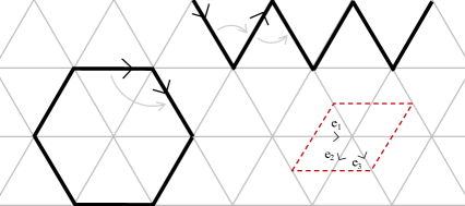
Figure 9. Triangular tiling. On the left: A simple closed polygonal chain that would be covered by applying $(\Lambda,L)=(C_{r},2m)$. On the top: A subset of a simple open polygonal chain that would be covered by applying $(\Lambda,L)=(B_{r},2m+1)$. On the right: A periodic cell with the vertex and edges labelled.

3.2.2. Crossed curves and $m$-twisted double line covering: $(\Lambda,L)=(\mathit{C}_{r},m)$

Lemma 3.8.

If $(\Lambda,L)=(\mathit{C}_{r},m)$, then for all $i\in(1,...,k)$ a characteristic loop,

$$\Delta_{(C_{r},m)}=(\delta_{0}^{\pm},\delta_{1}^{\pm},\cdots,\delta_{k}^{\pm})_{(C_{r},m)},$$

is defined by the following iterative sequence if $m$ is an even integer,

$$\delta_{i}=(\delta_{i-1})_{2}\mbox{ and }\delta_{0}=(\delta_{k})_{2},$$ (3.3)

otherwise by,

$$\delta_{\,2i}=(\delta_{\,2i-1})_{2}\ \mbox{ , }\ \delta_{\,2i+1}=(\delta_{\,2i})_{-2}\mbox{ and }\delta_{0}=(\delta_{k})_{2},$$ (3.4)

where each $\delta_{i}$ is an edge of $P$ covered by a $m$-twisted double line.

Proof.

With the same notations, the strategy for this method is similar to the previous one. The main difference concerns the $m$-twisted double line covering. Indeed, the transformation of $P$ by the $(\mathit{C}_{r},m)$ method can possibly create close components, depending on the parity of the positive integer $m$ representing the number of twists between the two strands replacing each edge of $P$. Again, by Definition 3.3 and using the notations above, as well as Remark 3.2, we can state that,

• if $m$ is even, each curve constructed after transforming all the edges and vertices by $(\mathit{C}_{r},m)$ is an alternating union of a right strand, followed by a left strand, and so forth which cover edges that are consecutive second counterclockwise adjacent edge, at each vertex they cross.

• if $m$ is odd, each curve constructed after transforming all the edges and vertices by $(\mathit{C}_{r},m)$ is an alternating union of two consecutive right strands, followed by two consecutive left strands, and so forth. In this case, the consecutive edges forming the polygonal chain alternate between second counterclockwise adjacent edge and second clockwise adjacent edge from the previous one.

Thus, Definition 3.6 and the notations of Fig.  7 conclude the proof. $\Box$

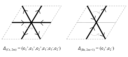
Figure 10. Periodic cell of a triangular tiling. On the left: Characteristic loop corresponding to Fig. 9 (left). On the right: Characteristic loop corresponding to Fig. 9 (top).

3.2.3. Branched curves and $m$-twisted double line covering: $(\Lambda,L)=(\mathit{B}_{r},m)$

Lemma 3.9.

If $(\Lambda,L)=(\mathit{B}_{r},m)$, then for all $i\in(1,...,k)$ a characteristic loop,

$$\Delta_{(B_{r},m)}=(\delta_{0}^{\pm},\delta_{1}^{\pm},\cdots,\delta_{k}^{\pm})_{(B_{r},m)},$$

is defined by the following iterative sequence if $m$ is an even integer,

$$\delta_{i}=(\delta_{i-1})_{1}\mbox{ and }\delta_{0}=(\delta_{k})_{1},$$ (3.5)

otherwise by,

$$\delta_{\,2i}=(\delta_{\,2i-1})_{1}\ \mbox{ , }\ \delta_{\,2i+1}=(\delta_{\,2i})_{-1}\mbox{ and }\delta_{0}=(\delta_{k})_{1},$$ (3.6)

where each $\delta_{i}$ is an edge of $P$ covered by a $m$-twisted double line.

Proof.

The proof follows directly from the one of Lemma 3.8 by replacing the second (counter-)clockwise adjacent edge by the first one in each case. $\Box$

3.3. Weaving, polycatenane or mixed motifs

Let $P$ be a $\mathcal{T}$-cell of a planar edge-to-edge doubly periodic tiling $\mathcal{T}$ and let $(\Lambda,L)$ be a polygonal link method. Then, since each curve component of a motif covers a characteristic loop in $P$, which is also a closed curve on a torus, we can identify its type by Definition 2.9.

Proposition 3.10.

A pair $\big{(}P,(\Lambda,L)\big{)}$ will generate

1. a polycatenane motif if and only if all the characteristic loops in $P$ are null-homotopic closed curve without trivial divided curves on $T^{2}$.

2. a mixed motif if and only if the set of all the characteristic loops in $P$ contains at least a null-homotopic and an essential closed curves without trivial divided curves.

3. a weaving motif if and only if all the characteristic loops in $P$ are homotopic to essential closed curves without trivial divided curves and such that at least two of them are non-parallel.
   

Proof.

The proof of this proposition is immediate and follows from Definition 2.9. Indeed up to isotopy, any weaving, polycatenane or mixed motif constructed from a polygonal method $(\Lambda,L)$ can have its components covering the edges of a $\mathcal{T}$-cell $P$. These curve components are essential and/or null-homotopic closed curves by definition, and if any curve admits a self-intersection point, then this point always divides it in two nontrivial components by Definition 2.8. Moreover, for a weaving motif, two of these curves are non-parallel by definition. Conversely, for a polygonal link method $(\Lambda,L)$, consider a set of characteristic loops on a $\mathcal{T}$-cell $P$ which does not admit null-homologous divided curves. If this set contains only null-homotopic closed curves, then $\big{(}P,(\Lambda,L)\big{)}$ is the scaffold of a polycatenane. If it contains at least a null-homotopic and an essential closed curve, then $\big{(}P,(\Lambda,L)\big{)}$ is the scaffold of a mixed motif. Finally, if the set contains only essential closed curves, such that two of them are non-parallel, then $\big{(}P,(\Lambda,L)\big{)}$ is the scaffold of a weaving motif. $\Box$

To identify if a characteristic loop on a torus $T^{2}$ satisfies the above conditions, we will use the polygonal description of each loop as an ordered sequence of oriented edges, detailed in the previous subsections, and prove our main theorem using algebraic arguments. Let $\pi_{1}(T^{2})$ be the fundamental group of the torus with generator $\alpha$ and $\beta$. Any closed curve on a torus can be described by a reduced cyclic torus word in $\pi_{1}(T^{2})$, and by commutativity of this fundamental group, the identity element is given by the trivial word $\alpha\beta\alpha^{-1}\beta^{-1}$, which thus characterizes a null-homotopic curve on $T^{2}$, as detailed in [12].

Definition 3.11.

Let $P$ be an arbitrary $\mathcal{T}$-cell and $(\Lambda,L)$ be a given polygonal link method. Let $S=(e_{1}^{+},e_{2}^{+},\cdots,e_{l}^{+})$ be the set of all edges of $P$ in the chosen positive direction, and let $F_{S}$ be the free group over $S$. Then, any characteristic loop $\Delta_{(\Lambda,L)}=(\delta_{0}^{\pm},\delta_{1}^{\pm},\cdots,\delta_{k}^{\pm})_{(\Lambda,L)}$ can be written as an edge word in $F_{S}$,

$$w=\delta_{0}^{\pm}.\delta_{1}^{\pm}.\cdots.\delta_{k}^{\pm}.$$

In particular, the edge word $w$ is said to be

• simple if for all $i,j\in\{1,\cdots,k\}$ distinct, $\delta_{i}\neq\delta_{j}$ and each pair of adjacent elements in $w$ have a distinct vertex in common,

• trivial if there exists a word $g$ in $F_{S}$ such that $w=g.g^{-1}$.

• knotted if there exists a word $g$ in $F_{S}$ such that $w=\delta_{0}^{\pm}.\cdots.\delta_{i}^{\pm}.g.\delta_{j}^{\pm}.\cdots.\delta_{k}^{\pm}$, with the edges $\delta_{i}$ and $\delta_{j}$ having a common vertex, which thus has degree four.

We illustrate this definition with the following example.

Example 3.12.

Let $P$ be a $\mathcal{T}$-cell of an hexagonal lattice and label and orient its edges as illustrated in Fig. 11. Note that this labeling is arbitrary.

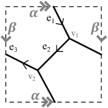
Figure 11. Periodic cell of an hexagonal tiling.

• To predict the type of motif created by applying $(\Lambda,L)=(\mathit{C}_{r},2)$ to $P$, one must list the characteristic loops covered by each strand after transformation, using the polygonal chain description given in Section 3.2.2. Here, in this first case, all the characteristic loop are equivalent, up to cyclic permutation and reversing of all orientations, to the following polygonal chain,

  $$\Delta_{(\mathit{C}_{r},2)}=(e_{1}^{+},e_{3}^{-},e_{2}^{-},e_{1}^{-},e_{3}^{+},e_{2}^{+})$$

  The symbols $\pm$ relate to the orientation of the edges given in Fig. 11, with a sign $+$ for the natural direction and $-$ for the reversed one. The corresponding trivial edge word is given by,

  $$w(\Delta_{(\mathit{C}_{r},2)})=e_{1}^{+}.e_{3}^{-}.e_{2}^{-}.e_{1}^{-}.e_{3}^{+}.e_{2}^{+},$$

  which is trivial. Indeed, following the torus orientation, the torus word $w^{\prime}(\Delta_{(\mathit{C}_{r},2)})$ of this cycle can be decomposed by the following,

  $$w^{\prime}(e_{1}^{+}.e_{3}^{-}) =\beta$$

  $$w^{\prime}(e_{3}^{-}.e_{2}^{-}.e_{1}^{-}) =\alpha$$

  $$w^{\prime}(e_{1}^{-}.e_{3}^{+}) =\beta^{-1}$$

  $$w^{\prime}(e_{3}^{+}.e_{2}^{+}.e_{1}^{+}) =\alpha^{-1}.$$

  Thus,

  $$w^{\prime}(\Delta_{(\mathit{C}_{r},2)})=\beta.\alpha.\beta^{-1}.\alpha^{-1}=0$$

  Moreover, this loop has a null-homotopic torus word. Therefore, by the following Theorem 3.13, we can conclude that the crossed curves and 2-twisted double line covering method applied to an hexagonal tiling will always generate a polycatenane. The same conclusion also holds for any even number of twists.

• for $(\Lambda,L)=(\mathit{B}_{r},3)$, we can describe all the characteristic loops by the following simple edge words, up to cyclic permutation and reversing all orientations,

  $$w(\Delta^{1}_{(\mathit{B}_{r},3)})=e_{1}^{+}.e_{3}^{-},$$

  $$w(\Delta^{2}_{(\mathit{B}_{r},3)})=e_{1}^{+}.e_{2}^{+},$$

  $$w(\Delta^{3}_{(\mathit{B}_{r},3)})=e_{3}^{+}.e_{2}^{+},$$

  Moreover, these characteristic loops have non-trivial and distinct torus words, namely $\beta$, $\alpha$ and $\beta^{-1}$, respectively. Thus, by Theorem 3.13, the branched curves and 3-twisted double line covering method applied to an hexagonal tiling will always generate a twisted weave. The same conclusion also holds for any odd number of twists.

Therefore, we can predict the type of motif that can be generated from a given $\mathcal{T}$-cell and a chosen polygonal link method in a general case.

Theorem 3.13.

(Motif Prediction Theorem)

Let $P$ be a $\mathcal{T}$-cell and $(\Lambda,L)$ be a polygonal link method. Then, $\big{(}P,(\Lambda,L)\big{)}$ generates

1. a weaving motif if and only if all the characteristic loops $\Delta_{(\Lambda,L)}$ in $P$ are essential, with at least two of them being non-parallel, and such that each of them has a word that can be written as a product of simple words,

2. a polycatenane motif if and only if each characteristic loops $\Delta_{(\Lambda,L)}$ in $P$ is null-homotopic and can be written as trivial word or as a product of simple words,

3. a mixed motif if and only if the set of all the characteristic loops $\Delta_{(\Lambda,L)}$ in $P$ contains at least an essential and a null-homotopic characteristic loops whose words can be written as trivial words and as a product of simple words.

Proof.

The indirect implications is immediate by definition. Then, for the direct implications, we can study separately the cases where a self-intersection on a characteristic loop is considered or not, namely, if the curve is simple or self-intersecting. First, we label all the edges and vertices of $P$ and assign to each edge an arbitrary orientation. For a chosen method $(\Lambda,L)$, define the edge word of a first characteristic loop $\Delta_{(\Lambda,L)}$, denoted by $w=w(\Delta_{(\Lambda,L)})$, using Definition 3.6 and the corresponding Lemmas 3.7,3.8,3.9. Recall that $w$ encodes the orientation of the edges with a sign $+$ or $-$, if the orientation of $\Delta_{(\Lambda,L)}$ follows the given orientation of the edge or not, respectively,

$$w=\delta_{0}^{\pm}.\delta_{1}^{\pm}.\cdots.\delta_{k}^{\pm}.$$

Moreover, considering non-simple characteristic loops, it is important to note that if an edge word contains twice the same edge in the same direction, then one of its endpoint lifts to a self-intersecting point on the corresponding characteristic loop if the polygonal link method transforms each edge by a double line twisting zero or an even number of times. However, for a characteristic loop intersecting the flat torus boundary, if the same condition than above holds for an odd number of twists, then the self-intersection point on the torus vanishes after lift. Finally, if an edge word contains twice the same edge in opposite direction, then if the polygonal link method transforms each by a double link without twist, then the characteristic loop is simple. Otherwise, it is self-intersecting.

Case 1: simple characteristic loops. If $w$ is a trivial or simple word, then $\Delta_{(\Lambda,L)}$ is a simple closed curve on the torus which thus lifts to a curve without self-intersection on $\mathbb{E}^{2}$. Thus, given the presentation of the torus considered above, one can assign a torus word $w^{\prime}=w^{\prime}(\Delta_{(\Lambda,L)})$ to $\Delta_{(\Lambda,L)}$ and deduce that the characteristic loop is essential or null-homotopic if $w^{\prime}$ is a nontrivial or trivial element of $\pi_{1}(T^{2})$, respectively. In particular, let $\alpha\beta\alpha^{-1}\beta^{-1}$ be the oriented flat torus boundary of $P$, with opposite sides characterized by the same symbol and oriented in opposite direction. Let $i$ and $j$ be two positive integers used to label the edges. Then, if an edge $\delta_{i}^{\pm}$ of $\Delta_{(\Lambda,L)}$ intersects the boundary $\alpha$ such that the orientation of the edge matches with (resp. is opposite to) the orientation given to $\beta$, then $\delta_{i}^{\pm}$ will be assigned the value $\beta$ (resp. $\beta^{-1}$) in $w^{\prime}$. The same holds by exchanging the roles of $\alpha$ and $\beta$. However, an edge $\delta_{j}^{\pm}$ of $\Delta_{(\Lambda,L)}$ that does not intersect any boundary of the flat torus will not contribute to $w^{\prime}$. Moreover, if $\Delta_{(\Lambda,L)}$ contains a subpath of connected ordered edges that do not intersect any flat torus boundary and whose edge word is simple, then its torus word is the identity and the subpath is said to be contractible. Thus, if none of the edges of $\Delta_{(\Lambda,L)}$ intersect a boundary of the flat torus, then its torus word is trivial and $\Delta_{(\Lambda,L)}$ is null-homotopic. Recall, that by commutativity of $\pi_{1}(T^{2})$, a torus word containing as many elements $\alpha$ (resp.$\beta$) as elements $\alpha^{-1}$ (resp. $\beta^{-1}$) is trivial. Therefore, if $\Delta_{(\Lambda,L)}$ is simple, then it is null-homotopic if $w^{\prime}$ is a trivial torus word on $\pi_{1}(T^{2})$ and if every characteristic loops satisfy these conditions, then $\big{(}P,(\Lambda,L)\big{)}$ generates a polycatenane motif by Definition 2.9. The converse holds immediately. Otherwise, if every characteristic loops have a non-trivial torus word, then they all are essential simple closed curves on $T^{2}$, and if at least two of them are non-parallel, then by Definition 2.9, $\big{(}P,(\Lambda,L)\big{)}$ generates a weaving motif. Once again the converse holds by definition. Finally, if the set of simple characteristic loops contains at least an essential one and a null-homotopic one, then $\big{(}P,(\Lambda,L)\big{)}$ generates a mixed motif.

Case 2: self-intersecting characteristic loops. If $\Delta_{(\Lambda,L)}$ contains any self-intersection point $p$, then $p$ is a vertex of degree four on the characteristic loop and separates it in two divided curves $\omega_{1}$ and $\omega_{2}$ intersecting in $p$. If $w$ is knotted, then at least one of $\omega_{1}$ or $\omega_{2}$ has a trivial torus word, or equivalently is null-homotopic, and $p$ is lifted to $\mathbb{E}^{2}$. Thus, since the corresponding curve component is not simple on $\mathbb{E}^{2}$, then the doubly periodic structure is neither a weave, a polycatenane nor a mixed diagram. Otherwise, $w$ is not knotted and the divided curves have edge words being either knotted or that can be decomposed as a product of simple words. Thus, $\omega_{1}$ and $\omega_{2}$ are not null-homologous, which implies that $p$ vanishes when lifting $\Delta_{(\Lambda,L)}$ to $\mathbb{E}^{2}$ as seen in Section 2.3, according to [28]. Therefore, $\big{(}P,(\Lambda,L)\big{)}$ generates one of the three type of entangled motif depending on the torus words of its characteristic loops as discussed in the first case above.

Finally, recall that even if the torus words of the characteristic loops depend on the choice of the generators of $\pi_{1}(\mathbb{(}T)^{2})$, as well as on the orientation and label of the elements $P$, the fact that these words are trivial or not is independent of this choice by definition of the mapping class group of the torus [12], and therefore does not affect our result, which concludes the proof of the theorem. $\Box$

Finally, we can end this section with some properties that can be proved immediately.

• For any $\mathcal{T}$-cell, $(\Lambda,L)=(\mathit{B}_{r},2m)$ always generates a polycatenane, with the particular case of an absence of crossings, namely a trivial structure, if $m=0$. This result generalizes to non-periodic tilings. Indeed, each tile is isotopic to a characteristic loop itself.

• Similarly, for any $\mathcal{T}$-cell such that all the vertices have degree 3, $(\Lambda,L)=(\mathit{C}_{r},2m)$ always generates a polycatenane by definition. This result generalizes to non-periodic tilings. Indeed, once again, each tile is isotopic to a characteristic loop itself.

• A characteristic loop isotopic to a polygonal chain containing parallel edges is essential by definition. Therefore, for any $\mathcal{T}$-cell such that all the vertices have degree 4, $(\Lambda,L)=(\mathit{C}_{r},2m)$ always generates a polycatenane by definition. This result generalizes to non-periodic tilings. Indeed, once again, each tile is isotopic to a characteristic loop itself.
  

4. Acknowledgements

We would like to thank K. Shimokawa (Ochanomizu University) and M. Chas (Stony Brook University) for their precious comments and advice during this study. This work is supported by a Research Fellowship from JST CREST Grant Number JPMJCR17J4 and Grant-in Aid for JSPS Fellows Number 22J13397.

References

- [1] C. Adams. The knot book: an elementary introduction to the mathematical theory of knots. (American Mathematical Society, Providence, 2004).
- [2] C. Adams, C. Albors-Riera, B. Haddock, Z. Li, D. Nishida, B. Reinoso, L. Wang. Hyperbolicity of links in thickened surfaces. Topology and Its Applications. 256 (2019), 262–278.
- [3] C. Adams, A. Calderon, N. Mayer. Generalized bipyramids and hyperbolic volumes of alternating k-uniform tiling links. Topology and Its Applications. 271 (2020),107045.
- [4] A. Champanerkar, I. Kofman, J.S. Purcell. Volume bounds for weaving knots. Algebr. Geom. Topol. 16 (2016), 3301–3323.
- [5] A. Champanerkar, I. Kofman, J.S. Purcell. Geometrically and diagrammatically maximal knots. J. London Math. Soc. 94 (2016), 883–908.
- [6] P.R. Cromwell. Knots and Links, 1st ed. (Cambridge University Press, 2004).
- [7] S. De Toffoli, V. Giardino. Forms and Roles of Diagrams in Knot Theory. Erkenn. 79 (2014), 829–842.
- [8] T. Endo, T. Itoh, K. Taniyama. A graph-theoretic approach to a partial order of knots and links. Topology and Its Applications. 157 (2010), 1002–1010.
- [9] M.E. Evans, V. Robins and S.T. Hyde. Periodic entanglement I: networks from hyperbolic reticulations. Acta Cryst. A69 (2013), 241–261.
- [10] M.E. Evans, V. Robins and S.T. Hyde. Periodic entanglement II: weavings from hyperbolic line patterns. Acta Cryst. A69 (1984), 262–275.
- [11] M.E. Evans and S.T. Hyde. Periodic entanglement III: tangled degree-3 finite and layer net intergrowths from rare forests. Acta Cryst. A71 (2015),599–611.
- [12] B. Farb and D. Margalit. A primer on mapping class groups. (Princeton University Press, Princeton, 2012).
- [13] Mizuki Fukuda, Motoko Kotani, Sonia Mahmoudi, Classification of doubly periodic untwisted (p,q)-weaves by their crossing number. To appear in J. Knot Theory Its Ramif..
- [14] S. Grishanov, V. Meshkov and A. Omelchenko. Kauffman-type polynomial invariants for doubly periodic structures. J. Knot Theory Its Ramif. 16 (2007),779–788.
- [15] B. Grünbaum and G.C. Shephard. Tilings and Patterns (second edition). (Dover Publications, Mineola, New York, 2016).
- [16] G. Hu, X.-D. Zhai, D. Lu and W.-Y. Qiu. The architecture of Platonic polyhedral links. J. Math. Chem. 46 (2009), 592–603.
- [17] S.T. Hyde, B. Chen and M. O’Keeffe. Some equivalent two-dimensional weavings at the molecular scale in 2D and 3D metal–organic frameworks. CrystEngComm. 18 (2016), 7607–7613.
- [18] S.T. Hyde, M.E. Evans. Symmetric tangled Platonic polyhedra. Proc. Natl. Acad. Sci. U.S.A. 119 (2022), e2110345118.
- [19] A. Kawauchi. Complexities of a knitting pattern. Reactive and Functional Polymers. 131 (2018) 230–236.
- [20] K. Kobata, T. Tanaka. A circular embedding of a graph in Euclidean 3-space. Topology and Its Applications. 157 (2010), 213–219.
- [21] Y. Liu, M. O’Keeffe, M.M.J. Treacy and O.M. Yaghi. The geometry of periodic knots, polycatenanes and weaving from a chemical perspective: a library for reticular chemistry. Chem. Soc. Rev. 47 (2018), 4642–4664.
- [22] D. Lu, G. Hu, Y.-Y. Qiu and W.-Y. Qiu. Topological transformation of dual polyhedral links. MATCH Commun. Math. Comput. Chem. 63 (2010), 67–78.
- [23] H.R. Morton, S.A. Grishanov. Doubly periodic textile structures. J. Knot Theory Ramifications. 18 (2009), 1597–1622.
- [24] K. Murasugi. Knot theory and its applications (Birkhäuser, Boston 2008).
- [25] E. Panagiotou, K.C. Millett, S. Lambropoulou, The linking number and the writhe of uniform random walks and polygons in confined spaces. J. Phys. A: Math. Theor. 43 (2010), 045208.
- [26] W.-Y. Qiu, X.-D. Zhai and Y.-Y. Qiu. Architecture of Platonic and Archimedean polyhedral links. J. Math. Chem. 51 (2008), 13–18.
- [27] K. Shimokawa, K. Ishihara, Y. Tezuka. Topology of polymers. (Springer Nature, Tokyo, 2019).
- [28] H. Tanio, O. Kobayashi. Rotation numbers for curves on a torus. Geom. Dedicata. 61 (1996), 1–9.
- [29] B. Thompson and S.T. Hyde. A theoretical schema for building weavings of nets via colored tilings of two-dimensional spaces and some simple polyhedral, planar and three-periodic examples. Isr. J. Chem. 58 (2018), 1144–1156.
- [30] N. Wakayama, K. Shimokawa. On the classification of polyhedral links. Symmetry. 14(8) (2022), 1712.