ER: Equivariance Regularizer for  Knowledge Graph Completion

Abstract

Tensor factorization and distanced based models play important roles in knowledge graph completion (KGC). However, the relational matrices in KGC methods often induce a high model complexity, bearing a high risk of overfitting. As a remedy, researchers propose a variety of different regularizers such as the tensor nuclear norm regularizer. Our motivation is based on the observation that the previous work only focuses on the “size” of the parametric space, while leaving the implicit semantic information widely untouched. To address this issue, we propose a new regularizer, namely, Equivariance Regularizer (ER), which can suppress overfitting by leveraging the implicit semantic information. Specifically, ER can enhance the generalization ability of the model by employing the semantic equivariance between the head and tail entities. Moreover, it is a generic solution for both distance based models and tensor factorization based models. The experimental results indicate a clear and substantial improvement over the state-of-the-art relation prediction methods.

Introduction

Knowledge Graph (KG) represents a collection of interlinked descriptions of entities, namely, real-world objects, events, and abstract concepts. Knowledge graphs are applied for a wide spectrum of applications ranging from question answering (Ramnath and Hasegawa-Johnson 2020), natural language processing (Zhang et al. 2019c), computer vision (Marino, Salakhutdinov, and Gupta 2017) and recommendation systems (Wang et al. 2018). However, the knowledge graph is usually incomplete with missing relations between entities. To predict missing links between entities based on known links effectively, a key step, known as Knowledge Graph Completion (KGC) has attracted increasing attention from the community.

There are mainly two important branches of KGC models: distance based (DB) models and tensor factorization based (TFB) models. As for the former, they use the Minkowski distance to calculate the similarity between vectors of entities, and they can achieve reasonable performance relying on the geometric significance. As for the latter, they treat knowledge graph completion as a tensor completion problem so that these models are highly expressive in theory. A noteworthy fact is that the relation-specific matrices in DB and TFB models contain lots of parameters, which can embrace rich potential relations. However, the performance of such models usually suffers from the overfitting problem since the relational matrices induce a high model complexity. For example, (Wang et al. 2017) has shown models such as RESCAL (Nickel, Tresp, and Kriegel 2011) are overfitting.

To address this challenge, researchers propose various regularizers. The squared Frobenius norm regularizer is a popular choice (Salakhutdinov and Srebro 2010a; Yang et al. 2015; Trouillon et al. 2016) for its convenience in applications. However, since the regularizer only imposes constraints to limit the parameter space (e.g., entities and relations), it cannot effectively improve the performance of some models with more implicit constraints (Ruffinelli, Broscheit, and Gemulla 2020) (e.g., RESCAL). Futhermore, (Lacroix, Usunier, and Obozinski 2018) proposes a tensor nuclear p-norm regularizer, which encourages to use the matrix trace norm in the matrix completion problem (Srebro, Rennie, and Jaakkola 2004; Candès and Recht 2009). Unfortunately, it is only suitable for canonical polyadic (CP) decomposition (Hitchcock and Frank 1927) based models such as ComplEx (Trouillon et al. 2016). For models with more complex mechanisms such as RESCAL (Nickel, Tresp, and Kriegel 2011), the tensor nuclear p-norm regularizer cannot utilize the potential semantic information so that it is weak in suppressing overfitting. Recently, (Zhang, Cai, and Wang 2020) proposes a regularizer called DURA for TFB models. It essentially imposes constraints on linked entities, which is deficient in exploring latent semantic relations. In summary, most of the aforementioned methods overlook the latent semantic relations and could only improve some specific models for KGC. How to find an efficient regularizer embracing both DB and TFB models remains wide open.

Figure 1: An illustration for the equivariance of proximity (left part in the figure) and dissimilarity (right part in the figure). $r$ denotes $relation$, $h_{i}$ denotes $head_{i}$ and $t_{i}$ denotes $tail_{i}$ ($i=1,2$).

In this paper, we propose a novel regularizer for both tensor factorization and distance based KGC models called Equivariance Regularizer (EA). As mentioned above, our motivation is based on the observation that previous work only focuses on limiting the parameter space, overlooking the potential semantic relation between entities. For example, given triples $(head_{1},relation,tail_{1})$ and $(head_{2},relation,tail_{2})$ shown in FIgure 1, if the semantics of $head_{1}$ and $head_{2}$ are similar, the semantics of $tail_{1}$ and $tail_{2}$ respectively linked by same $relation$ should be also similar generally, and vice versa. Motivated by this, different from previous work, we attempt to utilize the latent semantic information between entities to suppress overfitting, which can be realized on top of the equivariance of proximity and dissimilarity jointly. In light of this, ER can be applied to a variety of DB and TFB models, including RESCAL, ComplEx and RotatE (Sun et al. 2019). Experiments show that ER can yield consistent and significant improvements on datasets for the knowledge graph completion task.

Our contributions can be summarized as follows. (1) To the best of our knowledge, our regularizer is the first to focus on exploring potential semantic relations based on the equivariance of proximity and dissimilarity. (2) We provide a reformulation of our regularization, which shows the relationship between our work and traditional regularizers. Moreover, ER is a flexible regularizer that can be applied to both DB and TFB models. (3) We evaluate our model to address the challenge of relation prediction tasks for a wide variety of real-world datasets, and show that ER can produce sharp improvement on benchmarks.

Related Work

Knowledge graph embedding is an important research direction in representation learning. Therefore, a number of approaches have been developed for embedding KGs. We roughly divide previous KGC models into distance based models and tensor factorization based models.

Distance based (DB) models can model relations and entities by matrix or vector maps for a triple $(head,relation,tail)$. Specifically, Minkowski distance is applied to calculate the similarity between vectors of entities. Translational methods proposed first by TransE (Bordes et al. 2013) are widely used embedding methods, which interpret relation vectors as translations in vector space, i.e., $head+relation\approx tail$. A number of models aiming to improve TransE are proposed subsequently, such as TransH (Wang et al. 2014), TransR (Lin et al. 2015) and TransD (Ji et al. 2015). They use the score function like the formulation of $s(\bm{x}_{i},\bm{R}_{j},\bm{x}_{k})=-||f(\bm{x}_{i},\bm{R}_{j},\bm{x}_{k})||$, where $f$ is a model-specific function. Recently, there are some effective DB models proposed such as RotatE (Sun et al. 2019), RotH (Chami et al. 2020) and OTE (Tang et al. 2020), which have made great progress in the sense of geometric interpretation. However, some DB models (e.g., TransR (Lin et al. 2015)) have shortcomings in the expressive ability of the model since the DB models perform KGC based solely on observed facts rather than utilizing latent semantic information.

Tensor factorization based (TFB) models formulate the KGC task as a third-order binary tensor completion problem. Denote the head entity (tail entity) as $\bm{x}_{i}(\bm{x}_{k})$, and denote the matrix representing relation as $\bm{R}_{j}$. Suppose $\bm{Re}(\cdot)$ denotes the real part, and $\overline{\cdot}$ denotes the conjugate of a complex matrix. Then TFB models factorize the third-order tensor as $\bm{Re}(\overline{\bm{H}}\bm{R}_{j}\bm{T}^{\top})$. Specifically, the score functions are defined as $s(\bm{x}_{i},\bm{R}_{j},\bm{x}_{k})=\bm{Re}(\overline{\bm{x}}_{i}\bm{R}_{j}\bm{x}^{\top}_{k})$. RESCAL (Nickel, Tresp, and Kriegel 2011) proposes the three-way rank-r factorization over each relational slice of knowledge graph tensor. In this method a large amount of parameters are contained in the relation-specifific matrices and it bring a risk of overfifitting thereby. By restricting relation matrix to be diagonal for multi-relational representation learning, DistMult (Yang et al. 2015) proposes a simplified bilinear formulation but it cannot handle asymmetric relations. Going a step further, ComplEx (Trouillon et al. 2016) proposes to embed entities using complex vectors, which can capture symmetric and antisymmetric relations. Moreover, TuckER (Balažević, Allen, and Hospedales 2019c) learns embeddings by outputting a core tensor and embedding vectors of entities and relations. But due to the existence of overfitting (Nickel, Tresp, and Kriegel 2011), their performance lags behind the DB model. There are also some neural network models such as (Jin et al. 2021b), (Yu et al. 2021) (Jin et al. 2021a) and (Nathani et al. 2019), but they also have the risk of overfitting due to the huge number of parameters.

To tackle the overfitting problem of KGC models and enhance the performance of these models, researchers propose various regularizers. In the previous work, squared Frobenius norm ( L2 norm) regularizer is usually applied in TFB models (Nickel, Tresp, and Kriegel 2011; Yang et al. 2015; Trouillon et al. 2016). However, TFB models can not achieve comparable performance as distance based models (Sun et al. 2019; Zhang et al. 2019b). Then (Lacroix, Usunier, and Obozinski 2018) proposes to use the tensor nuclear 3-norm (Friedland and Lim 2014) (N3) as a regularizer. However, it is designed for some specific models such as ComplEx, and it is not appropriate for other general models such as RESCAL. Moreover, (Minervini et al. 2017a) uses a set of model-dependent soft constraints imposed on the predicate embeddings to model the equivalence and inversion patterns. There are also some methods such as (Ding et al. 2018; Minervini et al. 2017a, b) leveraging external background knowledge to achieve the regularization. (Guo et al. 2015) enforces the embedding space to be semantically smooth, i.e., entities belonging to the same semantic category will lie close to each other in the embedding space. (Xie, Liu, and Sun 2016) proposes that entities should have multiple representations in different types. In order to impose the prior belief for the structure in the embeddings space, (Ding et al. 2018) imposes approximate entailment constraints on relation embeddings and non-negativity constraints on entity embeddings. Recently, (Zhang, Cai, and Wang 2020) proposes the duality-induced regularizer for TFB models. However, it is derived from the score function of DB models, so it cannot significantly improve the performance of DB model.

Based on the survey above, so far, we can see that previous regularizers pay more attention to constraints of individual entities or relations rather than the latent semantics of the interaction between entities. Therefore, we attempt to design a regularizer applied for both DB and TFB models by employing the potential relations.

Methodology

In this section, we introduce a novel regularizer called Equivariance Regularizer (ER) for tensor factorization and distance based KGC models. Before introducing the methodology, we first provide a brief review of the knowledge graph completion. After that, we introduce the ER based on the equivariance of proximity and dissimilarity respectively, in which we explain their working mechanism. Then we propose the overall ER by integrating proximity and dissimilarity, and futher apply ER to knowledge graphs without entity categories. Finally, we give a theoretical analysis for the reformulation of ER.

Knowledge graph completion (KGC). Given a set $\mathcal{E}$ of entities and a set $\mathcal{R}$ of relations, a knowledge graph $\mathcal{G}\subseteq\mathcal{E}\times\mathcal{R}\times\mathcal{E}$ is a set of subject-predicate-object triples generally. A KGC model aims to predict missing links between entities based on known links automatically in the knowledge graph. For the convenience of expression, we denote embeddings of entities and relations as $\bm{x}_{i}$ (head entity) or $\bm{x}_{k}(\text{tail entity})\in\mathbb{R}^{d_{e}}$ and $\bm{R}_{j}\in\mathbb{R}^{d_{r}\times d_{r}}$ in a low-dimensional vector space, respectively; here $d_{e},d_{r}\in\mathbb{N}^{+}$ are the embedding size. Each particular model uses a scoring function $s$ to associate a score $s(i,k,j)$ with each potential triple $(i,j,k)\in\mathcal{E}\times\mathcal{R}\times\mathcal{E}$. Then we have the scoring function as $s(i,j,k)=f(\bm{x}_{i},\bm{R}_{j},\bm{x}_{k})$. The higher the score of a triple is, the more likely it is considered to be true by the model. Our goal is to predict true but unobserved triples based on the information in $\mathcal{G}$.

Generally, the score functions of the TFB and DB models are as follows, respectively: $f_{j}^{TFB}(i,j,k)=\boldsymbol{\operatorname{Re}}\left(\overline{\boldsymbol{x}}_{i}\boldsymbol{R}_{j}\boldsymbol{x}_{k}^{\top}\right)=\boldsymbol{\operatorname{Re}}\left(\left\langle\boldsymbol{x}_{i}\overline{\boldsymbol{R}}_{j},\boldsymbol{x}_{k}\right\rangle\right),f_{j}^{DB}(i,j,k)=-\left\|\boldsymbol{x}_{i}\mathbf{R}_{j}-\boldsymbol{x}_{k}\right\|,$ where $\bm{Re}(\cdot)$ denotes the real part of the complex number, and $\overline{\cdot}$ denotes the conjugate of a complex matrix.

Notice that the relation-specific matrices play important roles in modeling relations but meanwhile they may also carry some side effects. On one hand, the relation-specific matrices in TFB and DB models contain lots of parameters, which makes modeling complex relations available. On the other hand, increasing the model complexity also bears the risk of overfitting.

Researchers have proposed a series of regularizers to suppress overfitting. The basic paradigm of the regularized formulation is as follows:

$$\min\sum_{(\bm{x}_{i},\bm{R}_{j},\bm{x}_{k})\in\mathcal{S}}L\left(\bm{x}_{i},\bm{R}_{j},\bm{x}_{k}\right)+\lambda g(\bm{x}_{i},\bm{R}_{j},\bm{x}_{k}),$$ (1)

where $L\left(\cdot\right)$ represents the loss function in KGs, $\mathcal{S}$ is the set of triples in KGs, $\lambda$ is a fixed parameter, and $g(\cdot)$ is the regularization function.

Proximity Based Equivariance

Notice that the previous methods (e.g., (Guo et al. 2015), (Liu, Wu, and Yang 2017) (Xie, Liu, and Sun 2016), (Padia et al. 2019), (Minervini et al. 2017a)) pay more attention to explicit relational constraints, such as limiting the space of entities and relations. Unfortunately, the potential relational constraints such as multiple-hop space are not taken seriously. Therefore, we aim to utilize potential relations based on this perspective.

Let us take an example. As shown in Figure 2, London and Paris have similar semantics since they are all subordinate to the concept of capital (i.e., Paris is the capital of France and London is the capital of England). In this way, we expect that France and England linked by the same relation (capital$\_$of) should have similar semantics, since they are all subordinate to the concept of country. This suggests that embedding proximity is equivariant across head and tail entities, as expressed in the following assumption:

Assumption 1.

If $\bm{x}_{i}$ and $\bm{x}_{k}$ have similar semantics ($\boldsymbol{x}_{k}\stackrel{{\scriptstyle near}}{{\longrightarrow}}\boldsymbol{x}_{i}$), the entities $\bm{x}_{i}\boldsymbol{\overline{R}}_{j}$ and $\bm{x}_{k}\boldsymbol{\overline{R}}_{j}$ which are produced by $\bm{x}_{i}$ and $\bm{x}_{k}$ linking to the same relation $\boldsymbol{R}_{j}$, satisfy the equivariance of proximity ($\bm{x}_{k}\boldsymbol{\overline{R}}_{j}\stackrel{{\scriptstyle near}}{{\longrightarrow}}\bm{x}_{i}\boldsymbol{\overline{R}}_{j}$).

Motivated by this, we attempt to leverage the latent semantic relations in KGs to tackle the overfitting problem. First, for any entities $\boldsymbol{x}_{i}$ and $\boldsymbol{x}_{k}$ (e.g., London and Paris) which have similar semantics, we have the norm constraint:

$$\mathcal{R}_{1}=||\boldsymbol{x}_{i}||+||\boldsymbol{x}_{k}||,$$ (2)

where $||\cdot||$ can represent any norm of the vector. The function of the norm constraint here is to limit the embedding of entities in a similar semantic space.

Recall the given triples $(\bm{x}_{i},\bm{R}_{j_{1}},\bm{x}_{p})$ and $(\bm{x}_{k},\bm{R}_{j_{1}},\bm{x}_{q})$ in the example above. We can naturally deduce the the equivariance of proximity of $\boldsymbol{x}_{i}\overline{\mathbf{R}}_{j_{1}}$ (England) and $\boldsymbol{x}_{k}\overline{\mathbf{R}}_{j_{1}}$ (Franch) from $\bm{x}_{i}$ (London) and $\bm{x}_{k}$ (Paris) through the same relation $\mathbf{R}_{j_{1}}$ (capital$\_$of). Then we can seek such a semantics constraint on them to take into account the equivariance of proximity, which we name the proximity equivariance constraint:

$$\mathcal{R}_{2}=\sum_{i=1}^{n}\sum_{k=1}^{n}||\boldsymbol{x}_{i}\overline{\mathbf{R}}_{j_{1}}-\boldsymbol{x}_{k}\overline{\mathbf{R}}_{j_{1}}||a_{ik},$$ (3)

where $c_{\bm{x}_{i}}$ and $c_{\bm{x}_{k}}$ are the category labels of entities $\bm{x}_{i}$ and $\bm{x}_{k}$ respectively, and

$$a_{ik}=\left\{\begin{array}[]{ll}1,if\ c_{\bm{x}_{i}}=c_{\bm{x}_{k}},\\ 0,otherwise.\end{array}\right.$$ (4)

The function of the equivariant proximity constraint is to limit the embedding of link-derived entities to locate in a similar semantic space.

(a) A KG.

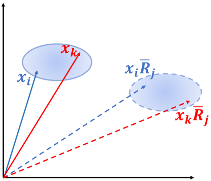
(b) Similar embeddings.

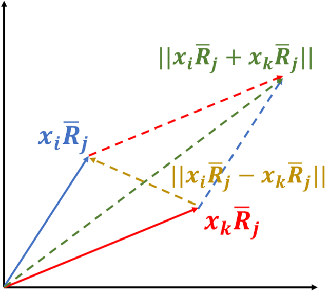
(c) ER.

Figure 2: An illustration of why ER can improve the performance of KGC models when the embedding dimensions are 2. Figure 2(a) shows that there are two triples (London, capital$\_$of, England) denoted as $(\boldsymbol{x}_{i},\boldsymbol{R}_{j},\boldsymbol{x}_{p})$ and (Paris, capital$\_$of, France) denoted as $(\boldsymbol{x}_{k},\boldsymbol{R}_{j},\boldsymbol{x}_{q})$. Figure 2(b) shows that if two entities are similar in semantics, the other entities connected to them through the same relation separately satisfy equivariant proximity in semantics. Figure 2(c) shows that ER can realize regularization function with $\|\boldsymbol{x}_{i}\overline{\mathbf{R}}_{j}-\boldsymbol{x}_{k}\overline{\mathbf{R}}_{j}||$ based on the equivariance of proximity, and realize regularization function with $\|\boldsymbol{x}_{i}\overline{\mathbf{R}}_{j}+\boldsymbol{x}_{k}\overline{\mathbf{R}}_{j}||$ based on the equivariance of dissimilarity, respectively.

Then the new model performs the embedding task by minimizing the following objective function:

$$\min\sum_{(\bm{x}_{i},\bm{R}_{j},\bm{x}_{k})\in\mathcal{S}}L\left(\bm{x}_{i},\bm{R}_{j},\bm{x}_{k}\right)+\lambda(\mathcal{R}_{1}+\mathcal{R}_{2}).$$ (5)

Dissimilarity Based Equivariance

We have proposed ER based on the equivariance of proximity between entities in the above. From another perspective, notice that not all head entities in triplets are semantically similar, i.e., some entities are semantically distant in the knowledge graph. Motivated by this, we will give another expression of ER based on the equivariance of dissimilarity.

Consider such an example. Given two triples (London, attribute$\_$of, city) and (Mississippi River, attribute$\_$of, river), $\bm{x}_{i}(\textbf{London})$ and $\bm{x}_{k}$ (Mississippi River) are not close in semantics, i.e., they are semantically distant. Since they have a public relation $\bm{R}_{j_{1}}$ (attribute$\_$of), we can infer that $\boldsymbol{x}_{i}\overline{\mathbf{R}}_{j_{1}}$ (city) and $\boldsymbol{x}_{k}\overline{\mathbf{R}}_{j_{1}}$ (river) satisfy the equivariance of dissimilarity in semantics. This suggests that embedding dissimilarity is equivariant across head and tail entities, as expressed in the following assumption:

Assumption 2.

if $\boldsymbol{x}_{i}$ and $\boldsymbol{x}_{k}$ are semantically distant $\boldsymbol{x}_{k}(\stackrel{{\scriptstyle far}}{{\longrightarrow}}\boldsymbol{x}_{i}$), the entities $\bm{x}_{i}\boldsymbol{\overline{R}}_{j}$ and $\bm{x}_{k}\boldsymbol{\overline{R}}_{j}$, which are produced by $\bm{x}_{i}$ and $\bm{x}_{k}$ linking to the same relation $\boldsymbol{R}_{j}$, should be equivariant dissimilarity ($\bm{x}_{k}\boldsymbol{\overline{R}}_{j}\stackrel{{\scriptstyle far}}{{\longrightarrow}}\bm{x}_{i}\boldsymbol{\overline{R}}_{j}$).

First of all, the semantic space of the entities should be bounded to ensure that it will not diverge, so we have the norm cosntraint $\mathcal{W}_{1}$ same as Eq.(2). Then we can notice such a fact as shown in Figure 2(c): the more futher the semantics of $\boldsymbol{x}_{i}\overline{\mathbf{R}}_{j_{1}}$ and $\boldsymbol{x}_{k}\overline{\mathbf{R}}_{j_{1}}$ are away from each other, the larger $||\boldsymbol{x}_{i}\overline{\mathbf{R}}_{j_{1}}-\boldsymbol{x}_{k}\overline{\mathbf{R}}_{j_{1}}||$ is, which means that $||\boldsymbol{x}_{i}\overline{\mathbf{R}}_{j_{1}}+\boldsymbol{x}_{k}\overline{\mathbf{R}}_{j_{1}}||$ will be smaller in the vector parallelogram for this case. We denote the labels of entity $\bm{x}_{i}$ and $\bm{x}_{k}$ as $c_{\bm{x}_{i}}$ and $c_{\bm{x}_{k}}$ respectively. Then we can use the following constraints as the dissimilarity equivariance constraint:

$$\mathcal{W}_{2}=\sum_{i=1}^{n}\sum_{k=1}^{n}||\boldsymbol{x}_{i}\overline{\mathbf{R}}_{j_{1}}+\boldsymbol{x}_{k}\overline{\mathbf{R}}_{j_{1}}||b_{ik},$$ (6)

where

$$b_{ik}=\left\{\begin{array}[]{ll}0,\ if\ c_{\bm{x}_{i}}=c_{\bm{x}_{k}},\\ 1,\ otherwise.\end{array}\right.$$ (7)

The objective function could then be formulated as follows:

$$\min\sum_{(\bm{x}_{i},\bm{R}_{j},\bm{x}_{k})\in\mathcal{S}}L\left(\bm{x}_{i},\bm{R}_{j},\bm{x}_{k}\right)+\lambda(\mathcal{W}_{1}+\mathcal{W}_{2}).$$ (8)

Joint Model Based Equivariance

In the above, we have applied ER to the knowledge graphs with predefined entity types. However, in fact, the entities in some knowledge graphs are not classified into different categories, so we cannot utilize their information about the entity type in this case. Therefore it motivates us to attempt to use a appropriate metric equivalently instead of using entity categories. Based on the observations above, we have the following assumption:

Assumption 3.

If two entities $\bm{x}_{i}$ and $\bm{x}_{k}$ have similar embeddings ($\boldsymbol{x}_{k}\stackrel{{\scriptstyle near}}{{\longrightarrow}}\boldsymbol{x}_{i}$), they may belong to the same semantic category ($c_{\bm{x}_{i}}=c_{\bm{x}_{k}}$).

To evaluate the similarity of two entities $\bm{x}_{i}$ and $\bm{x}_{k}$, we propose a discriminant for their embeddings approximately:

$$\left\{\begin{array}[]{c}c_{\bm{x}_{i}}=c_{\bm{x}_{k}},if\ ||\bm{x}_{i}-\bm{x}_{k}||\leq\epsilon_{j},\\ c_{\bm{x}_{i}}\neq c_{\bm{x}_{k}},if\ ||\bm{x}_{i}-\bm{x}_{k}||>\epsilon_{j},\end{array}\right.$$ (9)

where $\epsilon_{j}$ is the semantic-similarity parameter for each relation $\bm{R}_{j}$, which can be learned automatically in ER. Combining Eq.(9) with Eq.(4) and Eq.(7), we can apply ER to knowledge graphs without entity categories. Specifically, if $||\bm{x}_{i}-\bm{x}_{k}||\leq\epsilon_{j}$, we can use ER based on proximity equivariance; otherwise, we can use ER based on dissimilarity equivariance.

Moreover, we notice that there are some instances which does not fit the equivariance of proximity and dissimilarity. For example, two entities are close in semantics but their linking entities are not so close in semantics. Fortunately, ER can adjust $\epsilon_{j}$ appropriately larger automatically in order to make a trade-off. In this case, it can take into account differences of entities while capturing similarities.

In general, ER can handle knowledge graphs with and without category labels of entities, which provides a theoretical guarantee that the ER can be widely used in different knowledge graphs. Moreover, we will see ER can be widely adopted in various KGC models and achieve the competitive performance in the experimental part.

Theoretic Analysis for ER

We have derived the general form of the regularizer based on the equivariance of proximity and dissimilarity, respectively. Next, we take the some models using ER as an example to give the reformulation of the regularizer. First of all, we define the nuclear t-norm of a 3D tensor.

Definition 1.

In the knowledge graph completion problem, the tensor nuclear t-norm of $\hat{\mathcal{X}}$ is

$${\|\hat{\mathcal{X}}\|_{t}}=\min \left\{\sum_{d=1}^{D}\left\|\mathbf{p}_{:d}\right\|_{t}\left\|\mathbf{r}_{:d}\right\|_{t}\left\|\mathbf{q}_{:d}\right\|_{t}:\right.$$ (10)

$$\left.\hat{\mathcal{X}}=\sum_{d=1}^{D}\mathbf{p}_{:d}\otimes\mathbf{r}_{:d}\otimes\mathbf{q}_{:d}\right\},$$

where $D$ is the embedding dimension, $\bm{p}_{:d}$, $\bm{r}_{:d}$, and $\bm{q}_{:d}$ denote the $d$-th columns of $\bm{x}_{i}$, $\bm{R}_{j}$, and $\bm{x}_{k}$.

Then we have the following reformulations of ER based on the equivariance for the case of 2-norm. The conclusion for other models can be analogized accordingly.

Theorem 1.

Suppose that the model mechanism $\hat{\bm{X}}=\bm{x}_{i}\overline{\bm{R}}_{j}\bm{x}^{\top}_{k}$ for $j=1,2,\cdots,|\mathcal{R}|$, where $\bm{x}_{i},\bm{x}_{k}$ are real matrices, $\bm{R}_{j}$ is diagonal. Denote $\mathcal{S}$ as the set of triples in KGs. Then, the following equation holds

$$\frac{1}{\sqrt{|\mathcal{R}|}}{\min\sum_{(\boldsymbol{x}_{i},\boldsymbol{R}_{j},\boldsymbol{x}_{k})\in\mathcal{S}}}||\boldsymbol{x}_{i}||_{F}^{2}+||\boldsymbol{x}_{k}||_{F}^{2}+\|\boldsymbol{x}_{i}\mathbf{R}_{j}-\boldsymbol{x}_{k}\mathbf{R}_{j}||_{F}^{2}$$ (11)

$$=\|\hat{\mathcal{X}}\|_{2}$$

Proof.

Please see the AppendixA.

Theorem 2.

Suppose that the model mechanism $\hat{\bm{X}}=\bm{x}_{i}\overline{\bm{R}}_{j}-\bm{x}_{k}$ for $j=1,2,\cdots,|\mathcal{R}|$, where $\bm{x}_{i},\bm{x}_{k},\bm{R}_{j}$ are real matrices and $\bm{R}_{j}$ is diagonal. Then, the following equation holds

$${\frac{1}{2\sqrt{|\mathcal{R}|}}\min\sum_{(\boldsymbol{x}_{i},\boldsymbol{R}_{j},\boldsymbol{x}_{k})\in\mathcal{S}}||\boldsymbol{x}_{i}||_{F}^{2}+||\boldsymbol{x}_{k}||_{F}^{2}+\|\boldsymbol{x}_{i}\mathbf{R}_{j}+\boldsymbol{x}_{k}\mathbf{R}_{j}||_{F}^{2}}$$ (12)

$$=\|\hat{\mathcal{X}}\|_{2}$$

Proof.

Please see the AppendixB.

We have discussed the reformulation of the regularizer with the 2-norm ($t=2$ in Eq.(10)) above. It shows the relationship between ER and the tensor nuclear 2-norm regularizer. Notice that the norm-based regularization has been extensively studied in the context of matrix completion. The trace norm (or nuclear norm) has been proposed as a convex relaxation of the rank (Srebro, Rennie, and Jaakkola 2004) for matrix completion in the setting of rating prediction, with strong theoretical guarantees (Candès and Recht 2009). Then the weighted nuclear 3-norm $||\cdot||_{3}$ can be easily implemented by keeping the regularization terms corresponding to the sampled triples only. Therefore, based on the equivariance of proximity and dissimilarity respectively, we introduce reformulations of the regularizer with 3-norm ($t=3$ in Eq.(10)).

Theorem 3.

Suppose that the model mechanism $\hat{\bm{X}}=\bm{x}_{i}\overline{\bm{R}}_{j}\bm{x}^{\top}_{k}$ for $j=1,2,\cdots,|\mathcal{R}|$, where $\bm{x}_{i},\bm{x}_{k},\bm{R}_{j}$ are real matrices and $\bm{R}_{j}$ is diagonal. Then, the following equation holds

$${\frac{1}{\sqrt{|\mathcal{R}|}}\min\sum_{(\boldsymbol{x}_{i},\boldsymbol{R}_{j},\boldsymbol{x}_{k})\in\mathcal{S}}||\boldsymbol{x}_{i}||_{3}^{3}+||\boldsymbol{x}_{k}||_{3}^{3}+\|\boldsymbol{x}_{i}\mathbf{R}_{j}-\boldsymbol{x}_{k}\mathbf{R}_{j}||_{3}^{3}}$$ (13)

$$=\|\hat{\mathcal{X}}\|_{3}$$

Proof.

Please see the AppendixC.

Theorem 4.

Suppose that the model mechanism $\hat{\bm{X}}=\bm{x}_{i}\overline{\bm{R}}_{j}-\bm{x}_{k}$ for $j=1,2,\cdots,|\mathcal{R}|$, where $\bm{x}_{i},\bm{x}_{k},\bm{R}_{j}$ are real matrices and $\bm{R}_{j}$ is diagonal. Then, the following equation holds

$${\frac{1}{4\sqrt{|\mathcal{R}|}}\min\sum_{(\boldsymbol{x}_{i},\boldsymbol{R}_{j},\boldsymbol{x}_{k})\in\mathcal{S}}||\boldsymbol{x}_{i}||_{3}^{3}+||\boldsymbol{x}_{k}||_{3}^{3}+\|\boldsymbol{x}_{i}\mathbf{R}_{j}+\boldsymbol{x}_{k}\mathbf{R}_{j}||_{3}^{3}}$$ (14)

$$=\|\hat{\mathcal{X}}\|_{3}$$

Proof.

Please see the AppendixD.

We have given the reformulation of ER to the regularizer of 3-norm. It shows the relationship between ER and the tensor nuclear 3-norm regularizer. Moreover, we can see that ER based on the equivariance of proximity is a stronger constraint than ER based on the equivariance of dissimilarity. It means that ER based on the equivariance of proximity may be more conducive to improving the performance of the model than ER based on the equivariance of dissimilarity when the overfitting is severe. We will verify this conjecture in the experimental part.

Experiments

In this section, we first introduce the experimental settings and show main results. Then we conduct some ablation experiments.

Experimental Settings

Datasets Description: We conduct experiments on three widely used benchmarks, WN18RR (Dettmers et al. 2017), FB15K-237 (Dettmers et al. 2017) and YAGO3-10 (Mahdisoltani, Biega, and Suchanek 2013), of which the statistics are summarized in Table 7. WN18RR is a subset of WN18 (Bordes et al. 2013) and it embraces a hierarchical collection of relations between words. FB15K-237 is a subset of FB15K (Bordes et al. 2013), in which inverse relations are removed. YAGO3-10 is larger in scale.

Evaluation Protocol: Two popular evaluation metrics are used: Mean Reciprocal Rank (MRR) and Hit ratio with cut-off values (Hits@n,n = 1,10). MRR is the average inverse rank for correct entities. Hit@n measures the proportion of correct entities in the top $n$ entities. Following (Bordes et al. 2013), we report the filtered results to avoid possibly flawed evaluation.

Baselines: We compared ER with a number of strong baselines. For DB models, we report MuRP (Balažević, Allen, and Hospedales 2019a), RotatE (Sun et al. 2019), QuatE (Zhang et al. 2019a), DualE (Cao et al. 2021), HypER (Balažević, Allen, and Hospedales 2019b), REFE (Chami et al. 2020) and GC-OTE (Tang et al. 2020); For TFB models, we report TuckER (Balažević, Allen, and Hospedales 2019c), CP (Hitchcock and Frank 1927), DistMult (Yang et al. 2015) and ComplEx (Trouillon et al. 2016).

Implementation Details: Following (Ruffinelli, Broscheit, and Gemulla 2020), we adopt the cross entropy loss function for all compared models. We take Adagrad (Duchi, Hazan, and Singer 2011) as the optimizer in the experiment, and use grid search based on the performance of the validation datasets to choose the best hyperparameters. Specifically, we search learning rates in $\{0.5,0.1,0.05,0.01,0.005,0.001\}$, and search regularization coefficients in $\{0.001,0.005,0.01,0.05,0.1,0.5\}$. All models are trained for a maximum of 200 epochs.

As shown in (Salakhutdinov and Srebro 2010b) and (Lacroix, Usunier, and Obozinski 2018), the weighted versions of regularizers will usually have a better performance than the unweighted versions if we sample entries of the matrix or tensor non-uniformly. Therefore, in the experiments, we implement ER of 2-norm in a weighted way (note that we all use the version of ER with this setting if there is no special explanations in the experiments).

	WN18RR			FB15K-237			YAGO3-10
Models	MRR	Hits@1	Hits@10	MRR	Hits@1	Hits@10	MRR	Hits@1	Hits@10
DistMult	.430	.390	.490	.241	.155	.419	.340	.240	.540
ConvE	.430	.400	.520	.325	.237	.501	.440	.350	.620
MuRP	.481	.440	.566	.335	.243	.518	-	-	-
TuckER	.470	.443	.526	.358	.266	.544	-	-	-
CP	.438	.414	.485	.333	.247	.508	.567	.494	.698
RESCAL	.455	.419	.493	.353	.264	.528	.566	.490	.701
ComplEx	.460	.428	.522	.346	.256	.525	.573	.500	.703
RotatE	.476	.428	.571	.338	.241	.533	.495	.402	.670
QuatE	.488	.438	.580	.348	.248	.550	.571	.501	.705
DualE	492	.444	.581	.365	.268	.559	.575	.505	.710
REFE	.473	.430	.561	.351	.256	.541	.577	.503	.712
GC-OTE	.491	.442	.583	.361	.267	.550	-	-	-
ROTH	.496	.449	$\bm{.586}$	.344	.246	.535	.570	.495	.706
CP-ER	.482	.444	.557	.371	.275	.561	.584	.508	.712
RotatE-ER	.490	.445	.581	.352	.255	.547	.581	.505	.704
RESCAL-ER	.499	.458	.582	.373	.281	.554	.583	.509	.715
ComplEx-ER	.494	.453	.575	.374	.282	.563	.588	.515	.718

Table 1: Evaluation results on WN18RR, FB15k-237 and YAGO3-10 datasets. The best performance on each model are marked in bold and second best results are underlined.

Results

we can see that ER is an effective regularizer from Table 1. Due to the existence of overfitting, the performance of the TFB models is usually not as advantaged as the DB models. However, using ER, the performance of RESCAL and ComplEx has been significantly improved, and can exceed that of the DB models.

For the three datasets in the table, the size of WN18RR is the smallest since it has only 11 relations and about 86,000 training samples. Generally, if there are more parameters in a model, it is more likely to cause overfitting when it is applied to a dataset with a smaller size. Therefore, compared with other datasets, we predict that the improvement brought by ER on WN18RR is expected to be greater, and the experiment also proves this point. On WN18RR dataset, RESCAL gets an MRR score of 0.455, which is lower than ComplEx ($0.460$). However, incorporated with ER, RESCAL gets the $4.4\%$ improvement on MRR and finally attains $0.499$, which outperforms all compared models. Overfitting problem also exists on larger data sets and we can see that the performance of the model has been significantly improved after utilizing ER. We find that the application of ER can also bring stable and meaningful improvements to the model, which shows that ER can effectively suppress the overfitting.

Experiment Analysis

Ablation Study on Equivariance of Proximity. Recall we have given the expression of ER in the section of the methodology. Furthermore, given triples $(\boldsymbol{x}_{i}\overline{\mathbf{R}}_{j_{1}},\mathbf{R}_{j_{2}},?)$ and $(\boldsymbol{x}_{k}\overline{\mathbf{R}}_{j_{1}},\mathbf{R}_{j_{2}},?)$, if $\mathbf{R}_{j_{2}}$ (country_of) is a relation connected to the entities $\boldsymbol{x}_{i}\overline{\mathbf{R}}_{j_{1}}$ (England) and $\boldsymbol{x}_{k}\overline{\mathbf{R}}_{j_{1}}$ (Franch) respectively, we expect the embeddings of $\boldsymbol{x}_{i}\overline{\mathbf{R}}_{j_{1}}\overline{\mathbf{R}}_{j_{2}}$ (Europe) and $\boldsymbol{x}_{k}\overline{\mathbf{R}}_{j_{1}}\overline{\mathbf{R}}_{j_{2}}$ (Europe) locate in a similar region. Then we can derive the second order equivariance of proximity:

$$\mathcal{R}_{3}=||\boldsymbol{x}_{i}\overline{\mathbf{R}}_{j_{1}}\overline{\mathbf{R}}_{j_{2}}-\boldsymbol{x}_{k}\overline{\mathbf{R}}_{j_{1}}\overline{\mathbf{R}}_{j_{2}}||.$$ (15)

To take advantage of various semantic information, we integrate Eq.(15), Eq.(2) and Eq.(3), then we propose the regularization based on the second order equivariance of proximity as follows:

$$\min\sum_{(\bm{x}_{i},\bm{R}_{j},\bm{x}_{k})\in\mathcal{S}}L\left(\bm{x}_{i},\bm{R}_{j},\bm{x}_{k}\right)+\lambda\sum_{i=1}^{3}\mathcal{R}_{i}$$ (16)

where $\mathcal{R}_{i}$ represents the $i$-th order equivariance of proximity.

In order to explore the impact of $\mathcal{R}_{i}$, we implement an ablation study on different order equivariance of proximity for ComplEx in FB15K237. As shown in Table 8 in Appendix, ComplEx_i means ComplEx using $\mathcal{R}_{i}$. We can see that ComplEx₁ is significantly higher than ComplEx₀. With the increase of the semantics constraints, we can see that the effect of ComplEx₂ is also improving compared to ComplEx₁, but the improvements are not very significant. This shows that it may be more appropriate and concise to adopt ER with the firstr order equivariance of proximity as the regularizer.

Comparison to Other Regularizers. We compare ER to the squared Frobenius norm (FRO) regularizer, the tensor nuclear 3-norm regularizer and DURA regularizer. As stated in Table 9 in Appendix, we shows the performance of the four regularizers on three TFB models: CP, ComplEx, and RESCAL. Table 10 in Appendix shows the performance of four regularizers on two DB models: TransE and RotatE.

First of all, we can see that ER achieves the best performance and DURA regularizer achieves the second for TFB models, while ER achieves the best performance and N3 regularizer achieves the second for DB models. It illustrates that ER is more beneficial for both TFB and DB models than other regularizers. Overall, capturing semantic similarity can produce powerful and consistent improvements to DB and TFB models. It further proves the rationality that ER regularizer takes advantage of semantics order constraints. Specifically, for the previous KGC models such as ComplEx and RotatE, ER produces further improvements than the DURA and N3 regularizers. Overall, ER shows obvious advantages over other models by applying latent semantic relations so that it can bring consistent improvements to KGC models. And the results also demonstrate that ER is more effective than DURA, N3 and FRO regularizers.

Comparison to Other Semantic Constraint Models. We have noticed these models: (Guo et al. 2015) enforces the embedding space to be semantically smooth, which we denote as LLE; (Xie, Liu, and Sun 2016) suggests that entities should have multiple representations in different types, which we denote as RHE; (Padia et al. 2019) predicts knowledge graph fact via knowledge-enriched tensor factorization, which we denote as TFR; (Minervini et al. 2017a) regularize knowledge graph embeddings via equivalence and inversion axioms, which we denote as EIA; (Zhang et al. 2020) leverages the abundant linguistic knowledge from pretrained language models, which we denote as Pretrain. Here we compare them with ER as shown in Table 11 in Appendix. Some of them try to enforce semantically similar entities to have similar embedding vectors or exploit the analogical structures in a knowledge graph. However, the semantic information they use mostly based on first-order like Eq.(2). For the potential deeper semantic relation, such as Eq.(3) and Eq.(6) which they have not paid attention to. Moreover, some methods above are not suitable for knowledge graphs of unknown entity categories. Notice pretrain method can learn entity and relation representations via pretrained language models, but we can see that ER performs better than pretrain method, which show the importance of capturing the potential semantics in KGC.

Study for ER of 3-norm. In the experiments above, we mainly study the ER of 2-norm. Next, we conduct a comparative experiment on ER of 3-norm. As shown in Table 12 in Appendix, we can see ER of 3-norm can effectively improve the performance of the model, which is similar to the performance of ER of the 2-norm. This demonstrates that ER is a stable regularizer, and it is robust to applications in different norm scenarios.

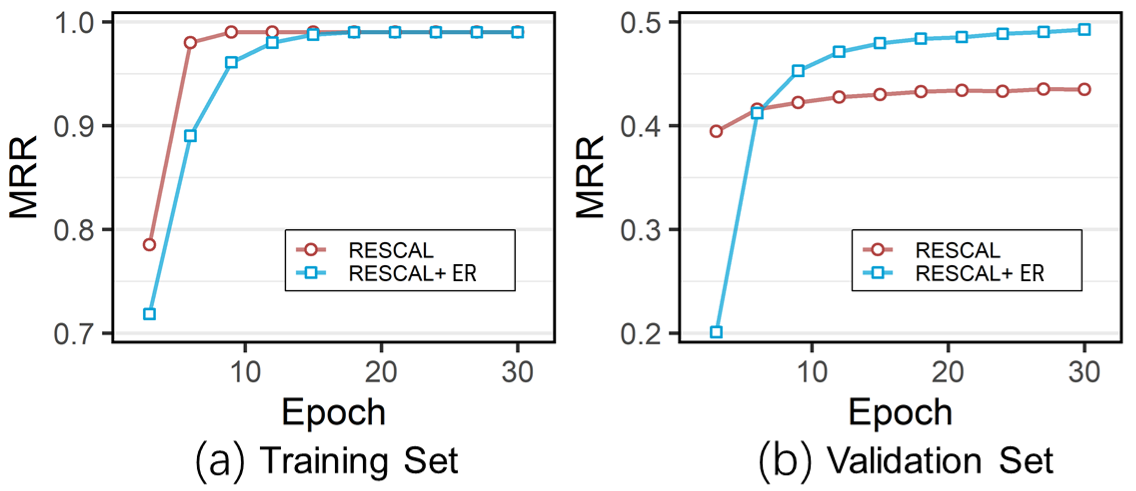
Figure 3: Study of training and validation curves.

Study of Training and Validation Curves. We conduct the research for RESCAL on training set and validation set of WN18RR. As shown in Figure 3 in Appendix, we can see that RESCAL without regularizer performs very well on the training set, but it performs poorly on the validation set, which shows that RECAL has a serious overfitting phenomenon. As the number of training epochs increases on the validation set, MRR of RESCAL without regularizer stops growing when it reaches around 0.455 while MRR of RESCAL with ER can reach 0.502. It demonstrates that ER can effectively suppresses overfitting and improve the generalization performance of the model.

Conclusion

We propose a widely applicable and effective regularizer named Equivariance Regularizer (ER) to suppress overfitting in KGE problem. It is based on the observation that the previous work only focuses on the similarity between entities while ignoring the latent semantic relation between them. Theoretically, ER can suppress overfitting and benefit the expressive ability of the model by utilizing the potential semantic information based on the equivariance of proximity and dissimilarity. All the results demonstrate that ER is more widely applicable than other regularizers. Experiments show that ER brings consistent and significant improvements to TFB and DB models on benchmark datasets.

Appendix

Appendix A Proof for Theorem 1

Theorem 1: Suppose that $\hat{\bm{X}}=\bm{x}_{i}\overline{\bm{R}}_{j}\bm{x}^{\top}_{k}$ for $j=1,2,\cdots,|\mathcal{R}|$, where $\bm{x}_{i},\bm{x}_{k},\bm{R}_{j}$ are real matrices and $\bm{R}_{j}$ is diagonal. Then, the following equation holds

$${\min}\frac{1}{\sqrt{|\mathcal{R}|}}\sum_{(\boldsymbol{x}_{i},\boldsymbol{R}_{j},\boldsymbol{x}_{k})\in\mathcal{S}}||\boldsymbol{x}_{i}||_{F}^{2}+||\boldsymbol{x}_{k}||_{F}^{2}+\|\boldsymbol{x}_{i}\mathbf{R}_{j}-\boldsymbol{x}_{k}\mathbf{R}_{j}||_{F}^{2}$$

$$=\|\hat{\mathcal{X}}\|_{2}.$$

Proof.

Notice that

$$\min\sum_{(\boldsymbol{x}_{i},\boldsymbol{R}_{j},\boldsymbol{x}_{k})\in\mathcal{S}}||\boldsymbol{x}_{i}||_{F}^{2}+||\boldsymbol{x}_{k}||_{F}^{2}+\|\boldsymbol{x}_{i}\mathbf{R}_{j}-\boldsymbol{x}_{k}\mathbf{R}_{j}||_{F}^{2}$$ (17)

$$\stackrel{{\scriptstyle a}}{{\leq}} \min\sum_{(\boldsymbol{x}_{i},\boldsymbol{R}_{j},\boldsymbol{x}_{k})\in\mathcal{S}}||\boldsymbol{x}_{i}||_{F}^{2}+||\boldsymbol{x}_{k}||_{F}^{2}+\|\boldsymbol{x}_{i}\mathbf{R}_{j}\|_{F}^{2}+\|\boldsymbol{x}_{k}\mathbf{R}_{j}||_{F}^{2}$$

$$-\|\boldsymbol{x}_{i}\mathbf{R}_{j}\boldsymbol{x}_{k}\mathbf{R}_{j}\|-\|\boldsymbol{x}_{k}\mathbf{R}_{j}\boldsymbol{x}_{i}\mathbf{R}_{j}\|$$

$$\leq \min\sum_{(\boldsymbol{x}_{i},\boldsymbol{R}_{j},\boldsymbol{x}_{k})\in\mathcal{S}}||\boldsymbol{x}_{i}||_{F}^{2}+||\boldsymbol{x}_{k}||_{F}^{2}+\|\boldsymbol{x}_{i}\mathbf{R}_{j}\|_{F}^{2}+\|\boldsymbol{x}_{k}\mathbf{R}_{j}||_{F}^{2}$$

$$-2\|\boldsymbol{x}_{i}\mathbf{R}_{j}\boldsymbol{x}_{k}\mathbf{R}_{j}\|_{F}^{2}$$

$$\leq \min\sum_{(\boldsymbol{x}_{i},\boldsymbol{R}_{j},\boldsymbol{x}_{k})\in\mathcal{S}}||\boldsymbol{x}_{i}||_{F}^{2}+||\boldsymbol{x}_{k}||_{F}^{2}+\|\boldsymbol{x}_{i}\mathbf{R}_{j}\|_{F}^{2}+\|\boldsymbol{x}_{k}\mathbf{R}_{j}||_{F}^{2}.$$

Since $\boldsymbol{x}_{i}\boldsymbol{R}_{j}$ and $\boldsymbol{x}_{k}\boldsymbol{R}_{j}$ are all vectors, we can have $\|\boldsymbol{x}_{i}\boldsymbol{R}_{j}\boldsymbol{x}_{k}\boldsymbol{R}_{j}\|=\|\boldsymbol{x}_{k}\boldsymbol{R}_{j}\boldsymbol{x}_{i}\boldsymbol{R}_{j}\|$. Then the inequality (a) holds.

We first prove that the following equation holds

$$\min_{\hat{X}_{j}=\boldsymbol{x}_{i}R_{j}x_{k}^{\top}}\frac{1}{\sqrt{|\mathcal{R}|}}\sum_{j=1}^{|\mathcal{R}|}\left(\|\boldsymbol{x}_{i}\|_{F}^{2}+\|\boldsymbol{x}_{k}\|_{F}^{2}+\left\|\boldsymbol{x}_{i}\boldsymbol{R}_{j}\right\|_{F}^{2}\right.$$ (18)

$$\left.+\|\boldsymbol{x}_{k}\boldsymbol{R}_{j}\|_{F}^{2}\right)=\|\hat{\mathcal{X}}\|_{2}.$$

Denote $\boldsymbol{x}_{i}$ as $\boldsymbol{p}$ and $\boldsymbol{x}_{k}$ as $\boldsymbol{q}$. Then we have that

$$\begin{aligned} &\sum_{j=1}^{|\mathcal{R}|}\left(\left\|\boldsymbol{x}_{i}\mathbf{R}_{j}\right\|_{F}^{2}+\|\boldsymbol{x}_{k}\|_{F}^{2}\right)\\ =&\sum_{j=1}^{|\mathcal{R}|}\left(\sum_{d=1}^{D}\left\|\mathbf{q}_{:d}\right\|_{F}^{2}+\sum_{i=1}^{I}\sum_{d=1}^{D}\mathbf{p}_{id}^{2}\mathbf{r}_{jd}^{2}\right)\\ =&\sum_{j=1}^{|\mathcal{R}|}\sum_{d=1}^{D}\left\|\mathbf{q}_{:d}\right\|_{2}^{2}+\sum_{d=1}^{D}\left\|\mathbf{p}_{:d}\right\|_{2}^{2}\left\|\mathbf{r}_{:d}\right\|_{2}^{2}\\ =&\sum_{d=1}^{D}\left(\left\|\mathbf{p}_{:d}\right\|_{2}^{2}\left\|\mathbf{r}_{:d}\right\|_{2}^{2}+|\mathcal{R}|\left\|\mathbf{q}_{:d}\right\|_{2}^{2}\right)\\ \geq&\sum_{d=1}^{D}2\sqrt{|\mathcal{R}|}\|\mathbf{p}_{:d}\left\|{}_{2}\right\|\mathbf{r}_{:d}\left\|{}_{2}\right\|\mathbf{q}_{:d}\|_{2}\\ =&2\sqrt{|\mathcal{R}|}\sum_{d=1}^{D}\left\|\mathbf{p}_{:d}\right\|_{2}\left\|\mathbf{r}_{:d}\right\|_{2}\left\|\mathbf{q}_{:d}\right\|_{2}\end{aligned}.$$

We can have the equality holds if and only if $\left\|\mathbf{p}_{:d}\right\|_{2}^{2}\left\|\mathbf{r}_{:d}\right\|_{2}^{2}=|\mathcal{R}|\left\|\mathbf{q}_{:d}\right\|_{2}^{2},$ i.e., $\left\|\mathbf{p}_{:d}\right\|_{2}\left\|\mathbf{r}_{:d}\right\|_{2}=\sqrt{|\mathcal{R}|}\left\|\mathbf{q}_{:d}\right\|_{2}$.

For all CP decomposition $\hat{\mathcal{X}}=\sum_{d=1}^{D}\mathbf{p}_{:d}\otimes\mathbf{r}_{:d}\otimes\mathbf{q}_{:d}$, we can always let $\bm{p}^{\prime}_{:d}=\bm{p}_{:d}$, $\bm{r}^{\prime}_{:d}=\sqrt{\frac{\left\|\mathbf{q}_{d}\right\|_{2}\sqrt{|\mathcal{R}|}}{\left\|\mathbf{p}_{:d}\right\|_{2}\left\|\mathbf{r}_{:d}\right\|_{2}}}\mathbf{r}_{:d}$ and $\bm{q}^{\prime}_{:d}=\sqrt{\frac{\left\|\mathbf{p}_{:d}\right\|_{2}\left\|\mathbf{r}_{:d}\right\|_{2}}{\left\|\mathbf{q}_{\cdot d}\right\|_{2}\sqrt{|\mathcal{R}|}}}\mathbf{p}_{:d}$, then we have

$$\left\|\mathbf{p}_{:d}^{\prime}\right\|_{2}\left\|\mathbf{r}_{:d}^{\prime}\right\|_{2}=\sqrt{|\mathcal{R}|}\left\|\mathbf{q}_{:d}^{\prime}\right\|_{2},$$

and at the same time we make sure that $\hat{\mathcal{X}}=\sum_{d=1}^{D}\mathbf{p}_{:d}^{\prime}\otimes\mathbf{r}_{:d}^{\prime}\otimes\mathbf{q}_{:d}^{\prime}$. Then, we can have

$${\frac{1}{\sqrt{|\mathcal{R}|}}}\sum_{j=1}^{|\mathcal{R}|}\left\|\hat{\mathcal{X}}_{j}\right\|_{2} =\frac{1}{2\sqrt{|\mathcal{R}|}}\sum_{j=1}^{|\mathcal{R}|}\min_{\hat{\mathcal{X}}_{j}=\boldsymbol{x}_{i}\mathbf{R}_{j}\boldsymbol{x}_{k}^{\top}}\left(\left\|\boldsymbol{x}_{i}\mathbf{R}_{j}\right\|_{F}^{2}+\|\boldsymbol{x}_{k}\|_{F}^{2}\right)$$

$$\leq\frac{1}{2\sqrt{|\mathcal{R}|}}\min_{\hat{\mathcal{X}}_{j}=\boldsymbol{x}_{i}\mathbf{R}_{j}\boldsymbol{x}_{k}^{\top}}\sum_{j=1}^{|\mathcal{R}|}\left(\left\|\boldsymbol{x}_{i}\mathbf{R}_{j}\right\|_{F}^{2}+\|\boldsymbol{x}_{k}\|_{F}^{2}\right)$$

$$=\min_{\hat{\mathcal{X}}=\sum_{d=1}^{D}\mathbf{p}_{j}\otimes\mathbf{r}_{id}\otimes\mathbf{q}_{:d}}\sum_{d=1}^{D}\left\|\mathbf{p}_{:d}\right\|_{2}\left\|\mathbf{r}_{:d}\right\|_{2}\left\|\mathbf{q}_{:d}\right\|_{2}$$

$$=\|\hat{\mathcal{X}}\|_{2}.$$

And in the same manner, we can have that

$${\min}\frac{1}{\sqrt{|\mathcal{R}|}}\sum_{(\boldsymbol{x}_{i},\boldsymbol{R}_{j},\boldsymbol{x}_{k})\in\mathcal{S}}||\boldsymbol{x}_{i}||_{F}^{2}+||\boldsymbol{x}_{k}||_{F}^{2}+\|\boldsymbol{x}_{i}\mathbf{R}_{j}-\boldsymbol{x}_{k}\mathbf{R}_{j}||_{F}^{2}$$

$$=\|\hat{\mathcal{X}}\|_{2}.$$

We can have the equality holds if and only if $\left\|\mathbf{q}_{:d}\right\|_{2}\left\|\mathbf{r}_{:d}\right\|_{2}=\sqrt{|\mathcal{R}|}\left\|\mathbf{p}_{:d}\right\|_{2}$. Then we can see that the conclusion holds if and only if $\left\|\mathbf{p}_{:d}\right\|_{2}\left\|\mathbf{r}_{:d}\right\|_{2}=\sqrt{|\mathcal{R}|}\left\|\mathbf{q}_{:d}\right\|_{2}$ and $||\bm{q}_{:d}||_{2}||\bm{r}_{:,d}||_{2}=\sqrt{|\mathcal{R}|}\left\|\mathbf{p}_{:d}\right\|_{2},\forall d\in\{1,2,\ldots,D\}$. Then the proof of Theorem 1 completes.

Appendix B Proof for Theorem 2

Theorem 2. Suppose that $\hat{\bm{X}}=\bm{x}_{i}\overline{\bm{R}}_{j}\bm{x}^{\top}_{k}$ for $j=1,2,\cdots,|\mathcal{R}|$, where $\bm{x}_{i},\bm{x}_{k},\bm{R}_{j}$ are real matrices and $\bm{R}_{j}$ is diagonal. Then, the following equation holds

$${\min}\frac{1}{2\sqrt{|\mathcal{R}|}}\sum_{(\boldsymbol{x}_{i},\boldsymbol{R}_{j},\boldsymbol{x}_{k})\in\mathcal{S}}||\boldsymbol{x}_{i}||_{F}^{2}+||\boldsymbol{x}_{k}||_{F}^{2}+\|\boldsymbol{x}_{i}\mathbf{R}_{j}+\boldsymbol{x}_{k}\mathbf{R}_{j}||_{F}^{2}$$

$$=\|\hat{\mathcal{X}}\|_{2}.$$

Proof.

First we have

$${\min}\frac{1}{2\sqrt{|\mathcal{R}|}}\sum_{(\boldsymbol{x}_{i},\boldsymbol{R}_{j},\boldsymbol{x}_{k})\in\mathcal{S}}||\boldsymbol{x}_{i}||_{F}^{2}+||\boldsymbol{x}_{k}||_{F}^{2}+\|\boldsymbol{x}_{i}\mathbf{R}_{j}+\boldsymbol{x}_{k}\mathbf{R}_{j}||_{F}^{2}$$

$$\leq \min_{(\boldsymbol{x}_{i},\boldsymbol{R}_{j},\boldsymbol{x}_{k})\in\mathcal{S}}\frac{1}{2\sqrt{|\mathcal{R}|}}\sum_{j=1}^{|\mathcal{R}|}\|\boldsymbol{x}_{i}\|_{F}^{2}+\|\boldsymbol{x}_{k}\|_{F}^{2}+\left\|\boldsymbol{x}_{i}\boldsymbol{R}_{j}\right\|_{F}^{2}$$

$$+\|\boldsymbol{x}_{k}\boldsymbol{R}_{j}\|_{F}^{2}+\|\boldsymbol{x}_{i}\boldsymbol{R}_{j}\boldsymbol{x}_{k}\boldsymbol{R}_{j}\|+\|\boldsymbol{x}_{k}\boldsymbol{R}_{j}\boldsymbol{x}_{i}\boldsymbol{R}_{j}\|$$

$$\stackrel{{\scriptstyle a}}{{=}} \min_{(\boldsymbol{x}_{i},\boldsymbol{R}_{j},\boldsymbol{x}_{k})\in\mathcal{S}}\frac{1}{2\sqrt{|\mathcal{R}|}}\sum_{j=1}^{|\mathcal{R}|}\|\boldsymbol{x}_{i}\|_{F}^{2}+\|\boldsymbol{x}_{k}\|_{F}^{2}+\left\|\boldsymbol{x}_{i}\boldsymbol{R}_{j}\right\|_{F}^{2}$$

$$+\|\boldsymbol{x}_{k}\boldsymbol{R}_{j}\|_{F}^{2}+2\|\boldsymbol{x}_{i}\boldsymbol{R}_{j}\boldsymbol{x}_{k}\boldsymbol{R}_{j}\|$$

$$\leq \min_{(\boldsymbol{x}_{i},\boldsymbol{R}_{j},\boldsymbol{x}_{k})\in\mathcal{S}}\frac{1}{2\sqrt{|\mathcal{R}|}}\sum_{j=1}^{|\mathcal{R}|}\|\boldsymbol{x}_{i}\|_{F}^{2}+\|\boldsymbol{x}_{k}\|_{F}^{2}+\left\|\boldsymbol{x}_{i}\boldsymbol{R}_{j}\right\|_{F}^{2}$$

$$+\|\boldsymbol{x}_{k}\boldsymbol{R}_{j}\|_{F}^{2}+\left\|\boldsymbol{x}_{i}\boldsymbol{R}_{j}\right\|_{F}^{2}+\|\boldsymbol{x}_{k}\boldsymbol{R}_{j}\|_{F}^{2}$$

$$\leq \min_{(\boldsymbol{x}_{i},\boldsymbol{R}_{j},\boldsymbol{x}_{k})\in\mathcal{S}}\frac{1}{2\sqrt{|\mathcal{R}|}}\sum_{j=1}^{|\mathcal{R}|}\|\boldsymbol{x}_{i}\|_{F}^{2}+\|\boldsymbol{x}_{k}\|_{F}^{2}+2\left\|\boldsymbol{x}_{i}\boldsymbol{R}_{j}\right\|_{F}^{2}$$

$$+2\|\boldsymbol{x}_{k}\boldsymbol{R}_{j}\|_{F}^{2}$$

$$\leq \min_{(\boldsymbol{x}_{i},\boldsymbol{R}_{j},\boldsymbol{x}_{k})\in\mathcal{S}}{\frac{1}{\sqrt{|\mathcal{R}|}}}\sum_{j=1}^{|\mathcal{R}|}\|\boldsymbol{x}_{i}\|_{F}^{2}+\|\boldsymbol{x}_{k}\|_{F}^{2}+\left\|\boldsymbol{x}_{i}\boldsymbol{R}_{j}\right\|_{F}^{2}+\|\boldsymbol{x}_{k}\boldsymbol{R}_{j}\|_{F}^{2}$$

Since $\boldsymbol{x}_{i}\boldsymbol{R}_{j}$ and $\boldsymbol{x}_{k}\boldsymbol{R}_{j}$ are all vectors, we can have $\|\boldsymbol{x}_{i}\boldsymbol{R}_{j}\boldsymbol{x}_{k}\boldsymbol{R}_{j}\|=\|\boldsymbol{x}_{k}\boldsymbol{R}_{j}\boldsymbol{x}_{i}\boldsymbol{R}_{j}\|$. Then the equality (a) holds.

Then in the same manner with Eq.(18), we can have that

$$\min{\frac{1}{2\sqrt{|\mathcal{R}|}}}\sum_{(\boldsymbol{x}_{i},\boldsymbol{R}_{j},\boldsymbol{x}_{k})\in\mathcal{S}}||\boldsymbol{x}_{i}||_{F}^{2}+||\boldsymbol{x}_{k}||_{F}^{2}+\|\boldsymbol{x}_{i}\mathbf{R}_{j}+\boldsymbol{x}_{k}\mathbf{R}_{j}||_{F}^{2}$$

$$=\|\hat{\mathcal{X}}\|_{2}.$$

We can have the equality holds if and only if $\left\|\mathbf{q}_{:d}\right\|_{2}\left\|\mathbf{r}_{:d}\right\|_{2}=\sqrt{|\mathcal{R}|}\left\|\mathbf{p}_{:d}\right\|_{2}$. Then we can see that the conclusion holds if and only if $\left\|\mathbf{p}_{:d}\right\|_{2}\left\|\mathbf{r}_{:d}\right\|_{2}=\sqrt{|\mathcal{R}|}\left\|\mathbf{q}_{:d}\right\|_{2}$ and $||\bm{q}_{:d}||_{2}||\bm{r}_{:,d}||_{2}=\sqrt{|\mathcal{R}|}\left\|\mathbf{p}_{:d}\right\|_{2},\forall d\in\{1,2,\ldots,D\}$. Then the proof of Theorem 2 completes.

Appendix C Proof for Theorem 3

Here we denote $|\bm{x}|^{3}$ as $||\bm{x}||_{3}^{3}$ and denote $|\bm{x}|^{\frac{3}{2}}$ as $||\bm{x}||_{C}$. Then we have Theorem 3 and Theorem 4 with their proofs as follows:

Theorem 3 Suppose that $\hat{\bm{X}}=\bm{x}_{i}\overline{\bm{R}}_{j}\bm{x}^{\top}_{k}$ for $j=1,2,\cdots,|\mathcal{R}|$, where $\bm{x}_{i},\bm{x}_{k},\bm{R}_{j}$ are real matrices and $\bm{R}_{j}$ is diagonal. Then, the following equation holds

$$\frac{1}{\sqrt{|\mathcal{R}|}}{\min}\sum_{(\boldsymbol{x}_{i},\boldsymbol{R}_{j},\boldsymbol{x}_{k})\in\mathcal{S}}||\boldsymbol{x}_{i}||_{3}^{3}+||\boldsymbol{x}_{k}||_{3}^{3}+\|\boldsymbol{x}_{i}\mathbf{R}_{j}-\boldsymbol{x}_{k}\mathbf{R}_{j}||_{3}^{3}$$ (19)

$$=\|\hat{\mathcal{X}}\|_{3}$$

Proof.

Notice that

$$\min\sum_{(\boldsymbol{x}_{i},\boldsymbol{R}_{j},\boldsymbol{x}_{k})\in\mathcal{S}}||\boldsymbol{x}_{i}||_{3}^{3}+||\boldsymbol{x}_{k}||_{3}^{3}+\|\boldsymbol{x}_{i}\mathbf{R}_{j}-\boldsymbol{x}_{k}\mathbf{R}_{j}||_{3}^{3}$$

$$\leq \min\sum_{(\boldsymbol{x}_{i},\boldsymbol{R}_{j},\boldsymbol{x}_{k})\in\mathcal{S}}||\boldsymbol{x}_{i}||_{3}^{3}+||\boldsymbol{x}_{k}||_{3}^{3}+\|\boldsymbol{x}_{i}\mathbf{R}_{j}\|_{3}^{3}+\|\boldsymbol{x}_{k}\mathbf{R}_{j}||_{3}^{3}.$$

We first prove that the following equation holds

$$\min_{\hat{X}_{j}=\boldsymbol{x}_{i}R_{j}x_{k}^{\top}}{\frac{1}{\sqrt{|\mathcal{R}|}}}\sum_{j=1}^{|\mathcal{R}|}\left(\|\boldsymbol{x}_{i}\|_{3}^{3}+\|\boldsymbol{x}_{k}\|_{3}^{3}+\left\|\boldsymbol{x}_{i}\boldsymbol{R}_{j}\right\|_{3}^{3}+\|\boldsymbol{x}_{k}\boldsymbol{R}_{j}\|_{3}^{3}\right)$$ (20)

$$=\|\hat{\mathcal{X}}\|_{3}.$$

Denote $\boldsymbol{x}_{i}$ as $\boldsymbol{p}$ and $\boldsymbol{x}_{k}$ as $\boldsymbol{q}$. Then we have that

$$\begin{aligned} &\sum_{j=1}^{|\mathcal{R}|}\left(\left\|\boldsymbol{x}_{i}\mathbf{R}_{j}\right\|_{3}^{3}+\|\boldsymbol{x}_{k}\|_{3}^{3}\right)\\ =&\sum_{j=1}^{|\mathcal{R}|}\left(\sum_{d=1}^{D}\left\|\mathbf{q}_{:d}\right\|_{3}^{3}+\sum_{i=1}^{I}\sum_{d=1}^{D}\mathbf{p}_{id}^{3}\mathbf{r}_{jd}^{3}\right)\\ =&\sum_{j=1}^{|\mathcal{R}|}\sum_{d=1}^{D}\left\|\mathbf{q}_{:d}\right\|_{3}^{3}+\sum_{d=1}^{D}\left\|\mathbf{p}_{:d}\right\|_{3}^{3}\left\|\mathbf{r}_{:d}\right\|_{3}^{3}\\ =&\sum_{d=1}^{D}\left(\left\|\mathbf{p}_{:d}\right\|_{3}^{3}\left\|\mathbf{r}_{:d}\right\|_{3}^{3}+|\mathcal{R}|\left\|\mathbf{q}_{:d}\right\|_{3}^{3}\right)\\ \geq&\sum_{d=1}^{D}2\sqrt{|\mathcal{R}|}\|\mathbf{p}_{:d}\left\|{}_{C}\right\|\mathbf{r}_{:d}\left\|{}_{C}\right\|\mathbf{q}_{:d}\|_{C}\\ =&2\sqrt{|\mathcal{R}|}\sum_{d=1}^{D}\left\|\mathbf{p}_{:d}\right\|_{C}\left\|\mathbf{r}_{:d}\right\|_{C}\left\|\mathbf{q}_{:d}\right\|_{C}\end{aligned}.$$

We can have the equality holds if and only if $\left\|\mathbf{p}_{:d}\right\|_{3}^{3}\left\|\mathbf{r}_{:d}\right\|_{3}^{3}=|\mathcal{R}|\left\|\mathbf{q}_{:d}\right\|_{3}^{3},$ i.e., $\left\|\mathbf{p}_{:d}\right\|_{C}\left\|\mathbf{r}_{:d}\right\|_{C}=\sqrt{|\mathcal{R}|}\left\|\mathbf{q}_{:d}\right\|_{C}$.

For all CP decomposition $\hat{\mathcal{X}}=\sum_{d=1}^{D}\mathbf{p}_{:d}\otimes\mathbf{r}_{:d}\otimes\mathbf{q}_{:d}$, we can always let $\bm{p}^{\prime}_{:d}=\bm{p}_{:d}$, $\bm{r}^{\prime}_{:d}=\sqrt{\frac{\left\|\mathbf{q}_{d}\right\|_{C}\sqrt{|\mathcal{R}|}}{\left\|\mathbf{p}_{:d}\right\|_{C}\left\|\mathbf{r}_{:d}\right\|_{C}}}\mathbf{r}_{:d}$ and $\bm{q}^{\prime}_{:d}=\sqrt{\frac{\left\|\mathbf{p}_{:d}\right\|_{C}\left\|\mathbf{r}_{:d}\right\|_{C}}{\left\|\mathbf{q}_{\cdot d}\right\|_{C}\sqrt{|\mathcal{R}|}}}\mathbf{p}_{:d}$, then we have

$$\left\|\mathbf{p}_{:d}^{\prime}\right\|_{C}\left\|\mathbf{r}_{:d}^{\prime}\right\|_{C}=\sqrt{|\mathcal{R}|}\left\|\mathbf{q}_{:d}^{\prime}\right\|_{C},$$

and at the same time we make sure that that $\hat{\mathcal{X}}=\sum_{d=1}^{D}\mathbf{p}_{:d}^{\prime}\otimes\mathbf{r}_{:d}^{\prime}\otimes\mathbf{q}_{:d}^{\prime}$. Therefore, we can have

$$\frac{1}{\sqrt{|\mathcal{R}|}}\sum_{j=1}^{|\mathcal{R}|}\left\|\hat{\mathcal{X}}_{j}\right\|_{C}$$

$$= \frac{1}{2\sqrt{|\mathcal{R}|}}\sum_{j=1}^{|\mathcal{R}|}\min_{\hat{\mathcal{X}}_{j}=\boldsymbol{x}_{i}\mathbf{R}_{j}\boldsymbol{x}_{k}^{\top}}\left(\left\|\boldsymbol{x}_{i}\mathbf{R}_{j}\right\|_{3}^{3}+\|\boldsymbol{x}_{k}\|_{3}^{3}\right)$$

$$\leq \frac{1}{2\sqrt{|\mathcal{R}|}}\min_{\hat{\mathcal{X}}_{j}=\boldsymbol{x}_{i}\mathbf{R}_{j}\boldsymbol{x}_{k}^{\top}}\sum_{j=1}^{|\mathcal{R}|}\left(\left\|\boldsymbol{x}_{i}\mathbf{R}_{j}\right\|_{3}^{3}+\|\boldsymbol{x}_{k}\|_{3}^{3}\right)$$

$$= \min_{\hat{\mathcal{X}}=\sum_{d=1}^{D}\mathbf{p}_{j}\otimes\mathbf{r}_{id}\otimes\mathbf{q}_{:d}}\sum_{d=1}^{D}\left\|\mathbf{p}_{:d}\right\|_{C}\left\|\mathbf{r}_{:d}\right\|_{C}\left\|\mathbf{q}_{:d}\right\|_{C}$$

$$= \|\hat{\mathcal{X}}\|_{3}.$$

And in the same manner, we can have that

$${\min}\frac{1}{\sqrt{|\mathcal{R}|}}\sum_{(\boldsymbol{x}_{i},\boldsymbol{R}_{j},\boldsymbol{x}_{k})\in\mathcal{S}}||\boldsymbol{x}_{i}||_{3}^{3}+||\boldsymbol{x}_{k}||_{3}^{3}+\|\boldsymbol{x}_{i}\mathbf{R}_{j}-\boldsymbol{x}_{k}\mathbf{R}_{j}||_{3}^{3}$$

$$=\|\hat{\mathcal{X}}\|_{3}.$$

We can have that the equality holds if and only if $\left\|\mathbf{q}_{:d}\right\|_{C}\left\|\mathbf{r}_{:d}\right\|_{C}=\sqrt{|\mathcal{R}|}\left\|\mathbf{p}_{:d}\right\|_{C}$. Then we can see that the conclusion holds if and only if $\left\|\mathbf{p}_{:d}\right\|_{C}\left\|\mathbf{r}_{:d}\right\|_{C}=\sqrt{|\mathcal{R}|}\left\|\mathbf{q}_{:d}\right\|_{C}$ and $||\bm{q}_{:d}||_{C}||\bm{r}_{:,d}||_{C}=\sqrt{|\mathcal{R}|}\left\|\mathbf{p}_{:d}\right\|_{C},\forall d\in\{1,2,\ldots,D\}$. Then the proof of Theorem 3 completes.

Appendix D Proof for Theorem 4

Theorem 4 Suppose that $\hat{\bm{X}}=\bm{x}_{i}\overline{\bm{R}}_{j}\bm{x}^{\top}_{k}$ for $j=1,2,\cdots,|\mathcal{R}|$, where $\bm{x}_{i},\bm{x}_{k},\bm{R}_{j}$ are real matrices and $\bm{R}_{j}$ is diagonal. Then, the following equation holds

$${\frac{1}{4\sqrt{|\mathcal{R}|}}}\min\sum_{(\boldsymbol{x}_{i},\boldsymbol{R}_{j},\boldsymbol{x}_{k})\in\mathcal{S}}||\boldsymbol{x}_{i}||_{3}^{3}+||\boldsymbol{x}_{k}||_{3}^{3}+\|\boldsymbol{x}_{i}\mathbf{R}_{j}+\boldsymbol{x}_{k}\mathbf{R}_{j}||_{3}^{3}$$ (21)

$$=\|\hat{\mathcal{X}}\|_{3}$$

First we prove $\|\boldsymbol{x}_{i}\mathbf{R}_{j}\|^{2}|\boldsymbol{x}_{k}\mathbf{R}_{j}|+|\boldsymbol{x}_{i}\mathbf{R}_{j}|||\boldsymbol{x}_{k}\mathbf{R}_{j}||^{2}\leq\|\boldsymbol{x}_{i}\mathbf{R}_{j}\|_{3}^{3}+\|\boldsymbol{x}_{k}\mathbf{R}_{j}\|_{3}^{3}$ holds. Notice that $|\boldsymbol{x}_{i}\mathbf{R}_{j}|+|\boldsymbol{x}_{k}\mathbf{R}_{j}|\geq 0$ and $(|\boldsymbol{x}_{i}\mathbf{R}_{j}|-|\boldsymbol{x}_{k}\mathbf{R}_{j}|)^{2}\geq 0$. Then we have

$$(|\boldsymbol{x}_{i}\mathbf{R}_{j}|+|\boldsymbol{x}_{k}\mathbf{R}_{j}|)(|\boldsymbol{x}_{i}\mathbf{R}_{j}|-|\boldsymbol{x}_{k}\mathbf{R}_{j}|)^{2}\geq 0$$ (22)

$$(|\boldsymbol{x}_{i}\mathbf{R}_{j}|+|\boldsymbol{x}_{k}\mathbf{R}_{j}|)(|\boldsymbol{x}_{i}\mathbf{R}_{j}|-|\boldsymbol{x}_{k}\mathbf{R}_{j}|)(|\boldsymbol{x}_{i}\mathbf{R}_{j}|-|\boldsymbol{x}_{k}\mathbf{R}_{j}|)\geq 0$$

$$(|\boldsymbol{x}_{i}\mathbf{R}_{j}|^{2}-|\boldsymbol{x}_{k}\mathbf{R}_{j}|^{2})(|\boldsymbol{x}_{i}\mathbf{R}_{j}|-|\boldsymbol{x}_{k}\mathbf{R}_{j}|)\geq 0$$

Then we can derive the following formula:

$$|\boldsymbol{x}_{i}\mathbf{R}_{j}|^{2}(|\boldsymbol{x}_{i}\mathbf{R}_{j}|-|\boldsymbol{x}_{k}\mathbf{R}_{j}|)\geq |\boldsymbol{x}_{k}\mathbf{R}_{j}|^{2}(|\boldsymbol{x}_{i}\mathbf{R}_{j}|-|\boldsymbol{x}_{k}\mathbf{R}_{j}|)$$ (23)

$$|\boldsymbol{x}_{i}\mathbf{R}_{j}|^{3}-|\boldsymbol{x}_{i}\mathbf{R}_{j}|^{2}|\boldsymbol{x}_{k}\mathbf{R}_{j}|\geq |\boldsymbol{x}_{k}\mathbf{R}_{j}|^{2}|\boldsymbol{x}_{i}\mathbf{R}_{j}|-|\boldsymbol{x}_{i}\mathbf{R}_{j}|^{3}$$

$$\|{\boldsymbol{x}_{i}}\mathbf{R}_{j}\|_{3}^{3}+\|\boldsymbol{x}_{k}\mathbf{R}_{j}\|_{3}^{3}\geq \|{\boldsymbol{x}_{i}}\mathbf{R}_{j}\|^{2}|\boldsymbol{x}_{k}\mathbf{R}^{\top}_{j}|+|\boldsymbol{x}_{i}\mathbf{R}_{j}|||\boldsymbol{x}_{k}\mathbf{R}_{j}||^{2}$$

Then we have:

$${\min}\frac{1}{4\sqrt{|\mathcal{R}|}}\sum_{(\boldsymbol{x}_{i},\boldsymbol{R}_{j},\boldsymbol{x}_{k})\in\mathcal{S}}||\boldsymbol{x}_{i}||_{3}^{3}+||\boldsymbol{x}_{k}||_{3}^{3}+\|\boldsymbol{x}_{i}\mathbf{R}_{j}+\boldsymbol{x}_{k}\mathbf{R}_{j}||_{3}^{3}$$

$$\stackrel{{\scriptstyle a}}{{\leq}} \min_{(\boldsymbol{x}_{i},\boldsymbol{R}_{j},\boldsymbol{x}_{k})\in\mathcal{S}}\frac{1}{4\sqrt{|\mathcal{R}|}}\sum_{j=1}^{|\mathcal{R}|}\|\boldsymbol{x}_{i}\|_{3}^{3}+\|\boldsymbol{x}_{k}\|_{3}^{3}+\left\|\boldsymbol{x}_{i}\boldsymbol{R}_{j}\right\|_{3}^{3}$$

$$+\|\boldsymbol{x}_{k}\boldsymbol{R}_{j}\|_{3}^{3}+3\|\boldsymbol{x}_{i}\mathbf{R}_{j}\|^{2}|\boldsymbol{x}_{k}\mathbf{R}_{j}|+3|\boldsymbol{x}_{i}\mathbf{R}_{j}|||\boldsymbol{x}_{k}\mathbf{R}_{j}||^{2}$$

$$\stackrel{{\scriptstyle b}}{{\leq}} \min_{(\boldsymbol{x}_{i},\boldsymbol{R}_{j},\boldsymbol{x}_{k})\in\mathcal{S}}\frac{1}{4\sqrt{|\mathcal{R}|}}\sum_{j=1}^{|\mathcal{R}|}\|\boldsymbol{x}_{i}\|_{3}^{3}+\|\boldsymbol{x}_{k}\|_{3}^{3}+\left\|\boldsymbol{x}_{i}\boldsymbol{R}_{j}\right\|_{3}^{3}$$

$$+\|\boldsymbol{x}_{k}\boldsymbol{R}_{j}\|_{3}^{3}+3\left\|\boldsymbol{x}_{i}\boldsymbol{R}_{j}\right\|_{3}^{3}+3\|\boldsymbol{x}_{k}\boldsymbol{R}_{j}\|_{3}^{3}$$

$$\leq \min_{(\boldsymbol{x}_{i},\boldsymbol{R}_{j},\boldsymbol{x}_{k})\in\mathcal{S}}\frac{1}{4\sqrt{|\mathcal{R}|}}\sum_{j=1}^{|\mathcal{R}|}\|\boldsymbol{x}_{i}\|_{3}^{3}+\|\boldsymbol{x}_{k}\|_{3}^{3}+4\left\|\boldsymbol{x}_{i}\boldsymbol{R}_{j}\right\|_{3}^{3}$$

$$+4\|\boldsymbol{x}_{k}\boldsymbol{R}_{j}\|_{3}^{3}$$

$$\leq \min_{(\boldsymbol{x}_{i},\boldsymbol{R}_{j},\boldsymbol{x}_{k})\in\mathcal{S}}{\frac{1}{\sqrt{|\mathcal{R}|}}}\sum_{j=1}^{|\mathcal{R}|}\|\boldsymbol{x}_{i}\|_{3}^{3}+\|\boldsymbol{x}_{k}\|_{3}^{3}+\left\|\boldsymbol{x}_{i}\boldsymbol{R}_{j}\right\|_{3}^{3}+\|\boldsymbol{x}_{k}\boldsymbol{R}_{j}\|_{3}^{3}$$

Since $\boldsymbol{x}_{i}\boldsymbol{R}_{j}$ and $\boldsymbol{x}_{k}\boldsymbol{R}_{j}$ are all vectors, we can have $\|\boldsymbol{x}_{i}\boldsymbol{R}_{j}\boldsymbol{x}_{k}\boldsymbol{R}_{j}\|=\|\boldsymbol{x}_{k}\boldsymbol{R}_{j}\boldsymbol{x}_{i}\boldsymbol{R}_{j}\|$. Then the inequality (a) holds. The inequality (b) holds due to the Eq.(22).

Then in the same manner with Eq.(20), we can have that

$${\min}\frac{1}{4\sqrt{|\mathcal{R}|}}\sum_{(\boldsymbol{x}_{i},\boldsymbol{R}_{j},\boldsymbol{x}_{k})\in\mathcal{S}}||\boldsymbol{x}_{i}||_{3}^{3}+||\boldsymbol{x}_{k}||_{3}^{3}+\|\boldsymbol{x}_{i}\mathbf{R}_{j}+\boldsymbol{x}_{k}\mathbf{R}_{j}||_{3}^{3}$$

$$=\|\hat{\mathcal{X}}\|_{3}.$$

We can have that the equality holds if and only if $\left\|\mathbf{q}_{:d}\right\|_{C}\left\|\mathbf{r}_{:d}\right\|_{C}=\sqrt{|\mathcal{R}|}\left\|\mathbf{p}_{:d}\right\|_{C}$. Then we can see that the conclusion holds if and only if $\left\|\mathbf{p}_{:d}\right\|_{C}\left\|\mathbf{r}_{:d}\right\|_{C}=\sqrt{|\mathcal{R}|}\left\|\mathbf{q}_{:d}\right\|_{C}$ and $||\bm{q}_{:d}||_{C}||\bm{r}_{:,d}||_{C}=\sqrt{|\mathcal{R}|}\left\|\mathbf{p}_{:d}\right\|_{C},\forall d\in\{1,2,\ldots,D\}$. Then the proof of Theorem 4 completes.

Appendix E Experimental Details and Appendix

We implement our model using PyTorch and test it on a single GPU. Here Table 7 shows statistics of the datasets used in this paper. The hypermeters for CP, ComplEx, RESCAL RotatE models are shown in Table 2, Table 3, Table 4 and Table 5 respectively. We have counted the running time of each epoch for different models with ER in WN18RR as follows: CP with ER takes 58s, ComplEx with ER takes 84s and RESCAL with ER takes 73s.

Study on semantic-similarity hyperparameter $\epsilon$. In the experiments above, we provide the semantic-similarity parameter $\epsilon_{j}$ for each relation $\bm{R}_{j}$ in ER. To characterize the similarity between entities adequately and study the impact of $\epsilon$, here we also conduct another version of ER where we provide $\epsilon_{ik}$ for $a_{ik}$ (in Eq.(3)), which we denote as $ER*$. From Table 6, we can see $ER$ and $ER*$ have similar performance. It shows providing $\epsilon_{j}$ for each relation $\bm{R}_{j}$ in ER is proper.

Datasets	WN18RR	FB15K237	YAGO3-10
dimension	2000	2000	2000
batch size	100	100	500
learning rate	0.1	0.05	0.1

Table 2: Hyperparameters found by grid search for CP mdoel.

Datasets	WN18RR	FB15K237	YAGO3-10
dimension	2000	2000	2000
batch size	200	200	1000
learning rate	0.05	0.1	0.05

Table 3: Hyperparameters found by grid search for ComplEx mdoel.

Datasets	WN18RR	FB15K237	YAGO3-10
dimension	512	512	512
batch size	400	400	1000
learning rate	0.1	0.1	0.05

Table 4: Hyperparameters found by grid search for RESCAL mdoel.

Datasets	WN18RR	FB15K237	YAGO3-10
dimension	400	400	400
batch size	100	100	500
learning rate	0.1	0.05	0.05

Table 5: Hyperparameters found by grid search for RotatE mdoel.

Model	MRR	Hits@1	Hits@10
ComplEx-ER	.374	.282	.563
ComplEx-ER*	.375	.282	.565

Table 6: Evaluation results of $\epsilon$ on FB15K237.

Dataset	$\#$Entity	$\#$Relation	$\#$Training	$\#$Valid	$\#$Test
WN18RR	40,943	11	86,835	3,034	3,134
FB15K237	14,541	237	272,115	17,535	20,466
YAGO3-10	123,182	37	1,079,040	5,000	5,000

Table 7: Statistics of the datasets used in this paper.

Model	MRR	Hits@1	Hits@10
ComplEx0	.355	.263	.542
ComplEx1	.374	.282	.563
ComplEx2	.378	.284	.569

Table 8: Evaluation results on FB15K237.

	WN18RR			FB15K-237			YAGO3-10
Models	MRR	Hits@1	Hits@10	MRR	Hits@1	Hits@10	MRR	Hits@1	Hits@10
CP-FRO	.460	-	.480	.340	-	.510	.540	-	.680
CP-N3	.470	.430	.544	.354	.261	.544	.577	.505	.705
CP-DURA	.478	.441	.552	.367	.272	.555	.579	.506	.709
CP-ER	.482	.444	.557	.371	.275	.561	.584	.508	.712
ComplEx-FRO	.470	-	.540	.350	-	.530	.573	-	.710
ComplEx-N3	.489	.443	.580	.366	.271	.558	.577	.502	.711
ComplEx-DURA	.491	.449	.571	.371	.276	.560	.584	.511	.713
ComplEx-ER	.494	.453	.575	.374	.282	.563	.588	.515	.718
RESCAL-FRO	.397	.363	.452	.323	.235	.501	.474	.392	.628
RESCAL-DURA	.498	.455	.577	.368	.276	.550	.579	.505	.712
RESCAL-ER	.499	.458	.582	.373	.281	.554	.583	.509	.715

Table 9: Comparison between DURA, the squared Frobenius norm (FRO), and the nuclear 3-norm (N3) regularizers (N3 does not apply to RESCAL). The best performance on each model are marked in bold.

	WN18RR			FB15K-237			YAGO3-10
Models	MRR	Hits@1	Hits@10	MRR	Hits@1	Hits@10	MRR	Hits@1	Hits@10
TransE-FRO	.259	.105	.532	.327	.231	.519	.478	.377	.665
TransE-N3	.265	.107	.533	.328	.232	.518	.483	.385	.664
TransE-DURA	.260	.105	.531	.328	.233	.518	.475	.371	.666
TransE-ER	.268	.110	.536	.329	.235	.525	.489	.384	.669
RotatE-FRO	.481	.434	.572	.337	.242	.528	.570	.481	.680
RotatE-N3	.483	.440	.580	346	.251	.538	.574	.498	.701
RotatE-DURA	.487	.443	.580	.342	.246	.533	.567	.491	.702
RotatE-ER	.490	.445	.581	.352	.255	.547	.581	.505	.704

Table 10: Comparison between DURA, the squared Frobenius norm (FRO), and the nuclear 3-norm (N3) regularizers. The best performance on each model are marked in bold.

	WN18RR			FB15K-237			YAGO3-10
Models	MRR	Hits@1	Hits@10	MRR	Hits@1	Hits@10	MRR	Hits@1	Hits@10
ComplEx-RHE	.469	.430	.538	.348	.262	.542	.570	.501	.708
ComplEx-LLE	.477	.442	.551	.363	.271	.552	.576	.504	.701
ComplEx-TFR	.473	.441	.545	.358	.264	.541	.573	.502	.702
ComplEx-EIA	.463	.345	.542	.356	.266	.529	.573	.501	.703
ComplEx-Pretrain	.479	.440	.553	.353	.268	.533	.578	.502	.704
ComplEx-ER	.494	.453	.575	.374	.282	.563	.588	.515	.718

Table 11: Evaluation results of different models on WN18RR, FB15k-237 and YAGO3-10 datasets.

	WN18RR			FB15K-237			YAGO3-10
Models	MRR	Hits@1	Hits@10	MRR	Hits@1	Hits@10	MRR	Hits@1	Hits@10
CP-ER	.479	.441	.556	.371	.273	.560	.582	.506	.709
ComplEx-ER	.492	.452	.574	.371	.275	.560	.586	.514	.712

Table 12: Evaluation results of ER based on 3-norm on WN18RR, FB15k-237 and YAGO3-10 datasets.

References

• Balažević, Allen, and Hospedales (2019a) Balažević; Allen, C.; and Hospedales, T. 2019a. Multi-relational Poincaré Graph Embeddings. In NIPS, 4465–4475.
• Balažević, Allen, and Hospedales (2019b) Balažević, I.; Allen, C.; and Hospedales, T. M. 2019b. Hypernetwork knowledge graph embeddings. In ICANN, 553–565. Springer.
• Balažević, Allen, and Hospedales (2019c) Balažević, I.; Allen, C.; and Hospedales, T. M. 2019c. Tucker: Tensor factorization for knowledge graph completion. In EMNLP, 5185–5194.
• Bordes et al. (2013) Bordes, A.; Usunier, N.; Garcia-Duran, A.; Weston, J.; and Yakhnenko, O. 2013. Translating embeddings for modeling multi-relational data. In NIPS, 2787–2795.
• Candès and Recht (2009) Candès, E. J.; and Recht, B. 2009. Exact Matrix Completion via Convex Optimization. Found. Comput. Math., 9(6): 717–772.
• Cao et al. (2021) Cao, Z.; Xu, Q.; Yang, Z.; Cao, X.; and Huang, Q. 2021. Dual Quaternion Knowledge Graph Embeddings. In AAAI, 6894–6902.
• Chami et al. (2020) Chami, I.; Wolf, A.; Juan, D.-C.; Sala, F.; Ravi, S.; and Ré, C. 2020. Low-Dimensional Hyperbolic Knowledge Graph Embeddings. In ACL.
• Dettmers et al. (2017) Dettmers, T.; Minervini, P.; Stenetorp, P.; and Riedel, S. 2017. Convolutional 2D Knowledge Graph Embeddings. In AAAI, 1811–1818.
• Ding et al. (2018) Ding, B.; Wang, Q.; Wang, B.; and Guo, L. 2018. Improving Knowledge Graph Embedding Using Simple Constraints. In ACL, 110–121.
• Duchi, Hazan, and Singer (2011) Duchi, J.; Hazan, E.; and Singer, Y. 2011. Adaptive subgradient methods for online learning and stochastic optimization. Journal of machine learning research, 12(Jul): 2121–2159.
• Friedland and Lim (2014) Friedland, S.; and Lim, L. H. 2014. Nuclear Norm of Higher-Order Tensors. volume 87, 1.
• Guo et al. (2015) Guo, S.; Wang, Q.; Wang, B.; Wang, L.; and Guo, L. 2015. Semantically Smooth Knowledge Graph Embedding. In ACL, 84–94.
• Hitchcock and Frank (1927) Hitchcock; and Frank, L. 1927. The Expression of a Tensor or a Polyadic as a Sum of Products. volume 6, 164–189.
• Ji et al. (2015) Ji, G.; He, S.; Xu, L.; Liu, K.; and Zhao, J. 2015. Knowledge Graph Embedding via Dynamic Mapping Matrix. In ACL, 687–696.
• Jin et al. (2021a) Jin, D.; Huo, C.; Liang, C.; and Yang, L. 2021a. Heterogeneous Graph Neural Network via Attribute Completion. In WWW, 391–400.
• Jin et al. (2021b) Jin, D.; Yu, Z.; Jiao, P.; Pan, S.; Yu, P. S.; and Zhang, W. 2021b. A Survey of Community Detection Approaches: From Statistical Modeling to Deep Learning. IEEE Transactions on Knowledge and Data Engineering, DOI: 10.1109/TKDE.2021.3104155.
• Lacroix, Usunier, and Obozinski (2018) Lacroix, T.; Usunier, N.; and Obozinski, G. 2018. Canonical Tensor Decomposition for Knowledge Base Completion. In ICML, 2863–2872.
• Lin et al. (2015) Lin, Y.; Liu, Z.; Sun, M.; Liu, Y.; and Zhu, X. 2015. Learning entity and relation embeddings for knowledge graph completion. In AAAI, 2181–2187.
• Liu, Wu, and Yang (2017) Liu, H.; Wu, Y.; and Yang, Y. 2017. Analogical Inference for Multi-relational Embeddings. In ICML, 2168–2178. PMLR.
• Mahdisoltani, Biega, and Suchanek (2013) Mahdisoltani, F.; Biega, J.; and Suchanek, F. 2013. YAGO3: A Knowledge Base from Multilingual Wikipedias. In CIDR.
• Marino, Salakhutdinov, and Gupta (2017) Marino, K.; Salakhutdinov, R.; and Gupta, A. 2017. The More You Know: Using Knowledge Graphs for Image Classification. In CVPR, 20–28.
• Minervini et al. (2017a) Minervini, P.; Costabello, L.; Muñoz, E.; Novácek, V.; and Vandenbussche, P. 2017a. Regularizing Knowledge Graph Embeddings via Equivalence and Inversion Axioms. volume 10534, 668–683. Springer.
• Minervini et al. (2017b) Minervini, P.; Demeester, T.; Rocktschel, T.; and Riedel, S. 2017b. Adversarial Sets for Regularising Neural Link Predictors. In 33rd Conference on Uncertainty in Artificial Intelligence (UAI), 11-15 August 2017, Sydney, Australia.
• Nathani et al. (2019) Nathani, D.; Chauhan, J.; Sharma, C.; and Kaul, M. 2019. Learning Attention-based Embeddings for Relation Prediction in Knowledge Graphs. In ACL, 4710–4723.
• Nickel, Tresp, and Kriegel (2011) Nickel, M.; Tresp, V.; and Kriegel, H. P. 2011. A Three-Way Model for Collective Learning on Multi-Relational Data. In ICML.
• Padia et al. (2019) Padia, A.; Kalpakis, K.; Ferraro, F.; and Finin, T. 2019. Knowledge graph fact prediction via knowledge-enriched tensor factorization. J. Web Semant., 59.
• Ramnath and Hasegawa-Johnson (2020) Ramnath, K.; and Hasegawa-Johnson, M. 2020. Seeing is Knowing! Fact-based Visual Question Answering using Knowledge Graph Embeddings. CoRR, abs/2012.15484.
• Ruffinelli, Broscheit, and Gemulla (2020) Ruffinelli, D.; Broscheit, S.; and Gemulla, R. 2020. You CAN Teach an Old Dog New Tricks! On Training Knowledge Graph Embeddings. In ICLR.
• Salakhutdinov and Srebro (2010a) Salakhutdinov, R.; and Srebro, N. 2010a. Collaborative Filtering in a Non-Uniform World: Learning with the Weighted Trace Norm. In NIPS, 2056–2064.
• Salakhutdinov and Srebro (2010b) Salakhutdinov, R.; and Srebro, N. 2010b. Collaborative Filtering in a Non-Uniform World: Learning with the Weighted Trace Norm. 2056–2064.
• Srebro, Rennie, and Jaakkola (2004) Srebro, N.; Rennie, J. D. M.; and Jaakkola, T. S. 2004. Maximum-Margin Matrix Factorization. In NIPS, 1329–1336.
• Sun et al. (2019) Sun, Z.; Deng, Z.; Nie, J.; and Tang, J. 2019. RotatE: Knowledge Graph Embedding by Relational Rotation in Complex Space. In ICLR, 1–18.
• Tang et al. (2020) Tang, Y.; Huang, J.; Wang, G.; He, X.; and Zhou, B. 2020. Orthogonal Relation Transforms with Graph Context Modeling for Knowledge Graph Embedding. In ACL, 2713–2722.
• Trouillon et al. (2016) Trouillon, T.; Welbl, J.; Riedel, S.; Gaussier, E.; and Bouchard, G. 2016. Complex embeddings for simple link prediction. In ICML, 2071–2080.
• Wang et al. (2018) Wang, H.; Zhang, F.; Wang, J.; Zhao, M.; Li, W.; Xie, X.; and Guo, M. 2018. RippleNet: Propagating User Preferences on the Knowledge Graph for Recommender Systems. In CIKM, 417–426.
• Wang et al. (2017) Wang, Q.; Mao, Z.; Wang, B.; and Guo, L. 2017. Knowledge Graph Embedding: A Survey of Approaches and Applications. IEEE Trans. Knowl. Data Eng., 29(12): 2724–2743.
• Wang et al. (2014) Wang, Z.; Zhang, J.; Feng, J.; and Chen, Z. 2014. Knowledge graph embedding by translating on hyperplanes. In AAAI, 1112–1119.
• Xie, Liu, and Sun (2016) Xie, R.; Liu, Z.; and Sun, M. 2016. Representation Learning of Knowledge Graphs with Hierarchical Types. In IJCAI, 2965–2971.
• Yang et al. (2015) Yang, B.; Yih, W.; He, X.; Gao, J.; and Deng, L. 2015. Embedding Entities and Relations for Learning and Inference in Knowledge Bases. In ICLR, 1–13.
• Yu et al. (2021) Yu, Z.; Jin, D.; Liu, Z.; He, D.; Wang, X.; Tong, H.; and Han, J. 2021. AS-GCN: Adaptive Semantic Architecture of Graph Convolutional Networks for Text-Rich Networks. In ICDM.
• Zhang et al. (2019a) Zhang, S.; Tay, Y.; Yao, L.; and Liu, Q. 2019a. Quaternion knowledge graph embeddings. In NIPS, 2731–2741.
• Zhang, Cai, and Wang (2020) Zhang, Z.; Cai, J.; and Wang, J. 2020. Duality-Induced Regularizer for Tensor Factorization Based Knowledge Graph Completion. In NIPS.
• Zhang et al. (2019b) Zhang, Z.; Cai, J.; Zhang, Y.; and Wang, J. 2019b. Learning Hierarchy-Aware Knowledge Graph Embeddings for Link Prediction.
• Zhang et al. (2019c) Zhang, Z.; Han, X.; Liu, Z.; Jiang, X.; Sun, M.; and Liu, Q. 2019c. ERNIE: Enhanced Language Representation with Informative Entities. In ACL, 1441–1451.
• Zhang et al. (2020) Zhang, Z.; Liu, X.; Zhang, Y.; Su, Q.; Sun, X.; and He, B. 2020. Pretrain-KGEs: Learning Knowledge Representation from Pretrained Models for Knowledge Graph Embeddings.