Aggregated Multi-output Gaussian Processes with Knowledge Transfer Across Domains

Abstract

Aggregate data often appear in various fields such as socio-economics and public security. The aggregate data are associated not with points but with supports (e.g., spatial regions in a city). Since the supports may have various granularities depending on attributes (e.g., poverty rate and crime rate), modeling such data is not straightforward. This article offers a multi-output Gaussian process (MoGP) model that infers functions for attributes using multiple aggregate datasets of respective granularities. In the proposed model, the function for each attribute is assumed to be a dependent GP modeled as a linear mixing of independent latent GPs. We design an observation model with an aggregation process for each attribute; the process is an integral of the GP over the corresponding support. We also introduce a prior distribution of the mixing weights, which allows a knowledge transfer across domains (e.g., cities) by sharing the prior. This is advantageous in such a situation where the spatially aggregated dataset in a city is too coarse to interpolate; the proposed model can still make accurate predictions of attributes by utilizing aggregate datasets in other cities. The inference of the proposed model is based on variational Bayes, which enables one to learn the model parameters using the aggregate datasets from multiple domains. The experiments demonstrate that the proposed model outperforms in the task of refining coarse-grained aggregate data on real-world datasets: Time series of air pollutants in Beijing and various kinds of spatial datasets from New York City and Chicago.

1 Introduction

Aggregate data often appear in various fields such as socio-economics [1, 2], public security [3, 4], ecology [5], agricultural economics [6, 7], epidemiology [8], meteorology [9, 10], public health [11], urban planning [12], and remote sensing [13]. The aggregate data contain a pair of support and attribute. The support is a predefined unit for aggregation, such as a time bin and a spatial region. The attribute value is obtained by aggregating point-referenced data over the corresponding support (see Figure 1). For example, time series of air pollutant concentration gathered by low-cost sensors is associated with coarse-grained time bins (e.g., six hours) because the point-referenced data are averaged over the bin to alleviate possible noise effects. Another example is the city’s poverty rate collected via household surveys; the point-referenced data are aggregated over spatial regions (e.g., districts) to preserve privacy.

In this article, we suppose the situation where various aggregate datasets in multiple domains are available and consider the problem of inferring functions for respective attributes. Here, the domain indicates an input space; for example, the domain is one-dimensional when we are interested in time series, and it is two-dimensional when we consider spatial data obtained from a city. The problem setting for two-dimensional domains is illustrated in Figure 1. The estimated function can be used to make predictions of attributes at any point, which is significant in various applications, such as improving city environments [2, 4]. For instance, analyzing the spatial distribution of poverty in a city allows one to optimize the allocation of resources for remedial action.

This problem is challenging because the aggregated attributes are obtained at supports with various granularities, namely different shapes and sizes (see Figure 1). Learning is difficult, especially when the data are sparse, that is, they are associated with coarse-grained supports. In that case, one promising approach is joint modeling of all attributes; however, it is still not obvious how to establish dependences between aggregated attributes across multiple domains.

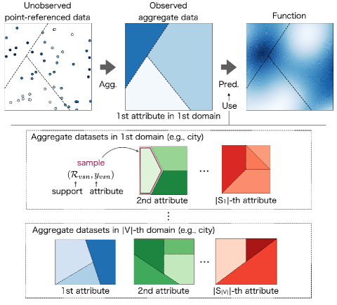
Figure 1: The problem setting when using aggregate datasets defined on two-dimensional domains. Darker hues represent higher attribute values. Assume that we obtain aggregate datasets in multiple domains, where each attribute value is given by aggregating point-referenced data over the corresponding support. Note that we do not use point-referenced data in either training or test phases. The goal is to infer a function for the attribute using aggregate datasets in multiple domains.

Gaussian processes (GPs) are nonparametric distributions over functions, which are widely used as priors to infer unknown functions from data [14]. Multi-output Gaussian processes (MoGPs) are promising to tackle the data sparsity issue, allowing one to learn functions by considering dependences between attributes [15]. However, almost all the GP-based models assume that the samples are obtained at points; they are not straightforwardly applicable to aggregate data observed at supports [16, 17, 18, 19, 20, 21, 22, 23].

This article presents a probabilistic model, called Aggregated Multi-output Gaussian Processes (A-MoGPs), to infer functions for attributes using aggregate datasets in multiple domains. In A-MoGP, the functions for attributes are assumed to be a dependent GP modeled as a linear mixing of independent latent GPs. The covariance functions of the latent GPs are shared among attributes and domains. By introducing a prior distribution of the mixing weights shared among domains, one can obtain appropriate estimates of the covariance functions and the weights via a knowledge transfer mechanism, even if some aggregate datasets have coarse granularities. The critical component of A-MoGP is to have an observation model with aggregation processes, in which attribute values are assumed to be calculated by integrating the mixed GP over the corresponding support. The covariances between supports are then given by the double integral of the covariance function over the corresponding pair of supports. This component is helpful because one can accurately evaluate the covariance between supports considering support shape and size.

The inference of A-MoGP is based on variational Bayes (VB). The model parameters can be learned by maximizing the evidence lower bound (ELBO), in which GPs are analytically integrated out. We adopt the reparameterization trick [24], which allows us to use gradient-based optimization methods for learning the variational parameters. By deriving the predictive distribution, we can obtain the functions for respective attributes considering the covariance of data points and the dependences between aggregated attributes simultaneously.

The main contributions of this article are as follows :

• We propose A-MoGP, a novel multi-output GP model that incorporates the aggregation process for each attribute in multiple domains.

• We develop a VB algorithm that can learn model parameters by maximizing the ELBO, in which latent GPs are analytically integrated out. This is the first derivation of the predictive distribution given aggregate datasets in multiple domains.

• The experiments on real-world datasets defined in temporal or spatial domains demonstrate the effectiveness of A-MoGP in the task of refining coarse-grained aggregate data.

This article is organized as follows: In Section 2, we describe related works. Section 3 describes aggregate datasets in multiple domains. In Section 4, we propose A-MoGP for inferring functions from aggregate datasets in multiple domains. In Section 5, we present the VB algorithm for learning model parameters and derive the predictive distribution. Section 6 demonstrates the effectiveness of A-MoGP using multiple real-world aggregate datasets. Finally, we describe concluding remarks and a discussion of future work in Section 7.

2 Related work

The problem of refining spatially aggregated data has long been addressed in the geostatistics community under the name of statistical downscaling, spatial disaggregation, and areal interpolation; the problem of predicting point-referenced data from aggregate data is also called the change of support problem [26]. One difficulty in these problems is that the covariance of aggregate data is not equal to that of point-referenced data, which is called the ecological fallacy [27, 28] in the field of statistics. In order to estimate the covariance from aggregate data precisely, it has been indicated that data aggregation processes should be incorporated into the models, as in prior works (e.g., [26, 29]) as well as in our proposal. The following paragraphs describe existing methods for addressing the problem we focus on, which can be roughly categorized into two approaches: Regression approach and multivariate approach.

A regression approach has been adopted frequently for refining coarse-grained aggregate data. This approach distinguishes multiple datasets into one target dataset and the others (auxiliary datasets) and then models the target attribute as a linear or non-linear mapping of the auxiliary attributes [30, 29, 5, 31, 32]. These models have the aggregation process only for the target attribute, encouraging consistency between the fine- and coarse-grained target attribute. The aggregation process is incorporated via block kriging [33] or transformations of Gaussian process (GP) priors [34, 35]. In recent years, regression-based models for aggregate settings have been studied in the field of machine learning [36, 37, 38, 39]. It has been pointed out that this task is a kind of multiple instance learning [36, 38]. The regression-based models assume that all the auxiliary datasets have sufficiently fine granularities (e.g., 5 minutes intervals in the timeline and 1 km $\times$ 1 km grid cells in the geographical space); thus they do not consider aggregation constraints for the auxiliary datasets. However, this assumption is not always fulfilled; for example, spatially aggregated datasets from cities are often associated with various geographical partitions such as districts and police precincts; hence, one might not be able to access fine-grained auxiliary datasets. In such cases, the regression-based approach cannot fully use all the aggregate datasets containing the coarse-grained ones.

An alternative for modeling multiple datasets is a multivariate approach. Unlike the regression approach, this approach does not distinguish multiple datasets; it aims to design a joint distribution of all attributes. Generally, the multivariate approach is expected to alleviate data sparsity issues. Multi-output Gaussian processes (MoGPs) [15] and co-kriging [40] are typical choices for modeling multivariate data that can consider covariances of data points and dependences between attributes simultaneously. Along the research line of MoGPs, there have been several sophisticated methods, including process convolution [18, 22] and latent factor modeling [16, 17, 19, 20, 21, 23], for establishing dependences between attributes. The linear model of coregionalization (LMC) is the general and most widely-used framework for constructing a multivariate function, in which outputs (i.e., attributes) are represented as a linear combination of independent latent functions [41, 42]. The MoGP models based on latent factor modeling are instances of LMC, where the latent functions are defined by GPs. Unfortunately, all the existing MoGP models cannot straightforwardly apply to the aggregate data this study focuses on because they assume point-referenced data. In other words, they do not have an important mechanism, that is, the aggregation constraints, for handling attributes aggregated over supports.

The proposed model is an extension of LMC. To handle the aggregate data, we introduce an observation model with the aggregation process for all attributes; this is represented by the integral of the MoGP over each corresponding support, as in [35]. We also present the variational Bayes algorithm for learning model parameters and derive the predictive distribution, given aggregate datasets in multiple domains. MoGP models for aggregate data have been independently proposed at the same time [43, 13, 25]. The main differences of ours from [43, 13] are as follows: (a) derivation of the predictive distribution given aggregate datasets from multiple domains; (b) knowledge transfer across domains by incorporating the prior distribution of mixing weights; (c) extensive experiments on real-world aggregate datasets gathered from temporal or spatial domains.

3 Aggregate Data

In this section, we introduce mathematical notations of aggregate datasets in multiple domains. Let $\mathcal{V}$ be a set of domain indices. Let $\mathcal{X}_{v}\subset\mathbb{R}^{D}(v\in\mathcal{V})$ be a domain of dimension $D$. In the case of $D=1$, a typical example of the domain is an observation time period; a domain example in the case of $D=2$ is a total region of a city. When we consider multiple domains, i.e., $|\mathcal{V}|\geq 2$, where $|\bullet|$ is the cardinality of the set, we regard that different domains do not intersect. Let $\bm{x}\in\mathcal{X}_{v}(v\in\mathcal{V})$ denote an input variable. Let $\mathcal{S}_{v}(v\in\mathcal{V})$ be a set of attribute indices for each domain. A partition $\mathcal{P}_{vs}(v\in\mathcal{V},s\in\mathcal{S}_{v})$ of $\mathcal{X}_{v}$ is a collection of disjoint subsets, called supports, of $\mathcal{X}_{v}$. Let $\mathcal{R}_{vsn}\in\mathcal{P}_{vs}$ be an $n$-th support in $\mathcal{P}_{vs}$. The support corresponds to the time bin ($D=1$), the spatial region ($D=2$), and so on. A data sample is specified by a pair $(\mathcal{R}_{vsn},y_{vsn})$, where $y_{vsn}\in\mathbb{R}$ is an attribute value that is observed by aggregating the point-referenced data over the corresponding support $\mathcal{R}_{vsn}$ (see Figure 1). Here, we assume that the aggregation process (e.g., averaging) for each attribute is known. Suppose that we have the collection of aggregate datasets $\mathcal{D}=\{\mathcal{D}_{v}\mid v\in\mathcal{V}\}$, where $\mathcal{D}_{v}=\{(\mathcal{R}_{vsn},y_{vsn})\mid s\in\mathcal{S}_{v};n=1,\ldots,|\mathcal{P}_{vs}|\}$. The notations used in this article are listed in Table I.

TABLE I: Notation of aggregate datasets.

Symbol	Description
$\mathcal{V}$	set of domain indices
$v$	domain index, $v\in\mathcal{V}$
$D$	dimension of domain, $D\in\mathbb{N}$
$\mathcal{X}_{v}$	$v$-th domain, $\mathcal{X}_{v}\subset\mathbb{R}^{D}$
$\mathcal{S}_{v}$	set of attribute indices for $v$-th domain
$s$	attribute index, $s\in\mathcal{S}_{v}$
$\mathcal{P}_{vs}$	partition of $\mathcal{X}_{v}$ for $s$-th attribute
$n$	support index, $n\in\{1,\ldots,|\mathcal{P}_{vs}|\}$
$\mathcal{R}_{vsn}$	support, $\mathcal{R}_{vsn}\in\mathcal{P}_{vs}$
$y_{vsn}$	attribute value associated with the support $\mathcal{R}_{vsn}$

4 Model

We propose A-MoGP (Aggregated Multi-output Gaussian Process), a probabilistic model for inferring functions from aggregate datasets with various granularities in multiple domains. The proposed model when we have two spatial domains is illustrated schematically in Figure 2. For simplicity, we assume that the types of attributes are the same for different domains; namely, we let $\mathcal{S}=\mathcal{S}_{v}$ denote the set of attribute indices for all domains. Notice that one can straightforwardly apply the proposed model to the case where the types of attributes are partially different across domains. In the following, we first construct a multi-output Gaussian process (MoGP) prior by linearly mixing independent latent GPs to establish dependences between attributes (see (a) Linear mixing in Figure 2). We then introduce a prior distribution of the mixing weights to transfer knowledge across domains (see (b) Prior dist. in Figure 2). Lastly, we present an observation model with aggregation processes for respective attributes (see (c) Agg. process in Figure 2), allowing a model learning from aggregate datasets.

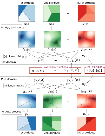
Figure 2: Schematic diagram of A-MoGP: Generative process of multiple aggregated attributes in two spatial domains. Covariance functions and prior distributions of weight parameters are shared among domains.

MoGP prior. In the proposed model, the functions for attributes on the continuous space are assumed to be an MoGP. We construct the MoGP by linearly mixing some independent latent GPs, which is one of the most widely used approaches for establishing dependences between outputs (i.e., attributes) [17, 15]. Let $\mathcal{L}$ be an index set of latent GPs. Consider $|\mathcal{V}||\mathcal{L}|$ independent zero-mean GPs,

$$g_{vl}(\bm{x}) \sim\mathcal{GP}\left(0,\gamma_{l}(\bm{x},\bm{x}^{\prime})\right),\quad v\in\mathcal{V};\,l\in\mathcal{L},$$ (1)

where $\gamma_{l}(\bm{x},\bm{x}^{\prime}):\mathbb{R}^{D}\times\mathbb{R}^{D}\to\mathbb{R}$ is a covariance function for the $l$-th latent GP, which is assumed integrable. It should be noted that the covariance functions $\{\gamma_{l}(\bm{x},\bm{x}^{\prime})\mid l\in\mathcal{L}\}$ are shared among all attributes and all domains, which enables us to effectively learn covariances of data points by utilizing dependences between attributes in multiple domains. Defining $f_{vs}(\bm{x})$ as the GP for the $s$-th attribute in the $v$-th domain, the $|\mathcal{S}|$-dimensional dependent GP $\bm{f}_{v}(\bm{x})=(f_{v1}(\bm{x}),\ldots,f_{v|\mathcal{S}|}(\bm{x}))^{\top}$ in the $v$-th domain is assumed to be modeled as a linear combination of the $|\mathcal{L}|$ independent latent GPs. The MoGP for the $v$-th domain is then given by

$$\bm{f}_{v}(\bm{x}) ={\bf W}_{v}\bm{g}_{v}(\bm{x}),$$ (2)

where $\bm{g}_{v}(\bm{x})=(g_{v1}(\bm{x}),\ldots,g_{v|\mathcal{L}|}(\bm{x}))^{\top}$, and where ${\bf W}_{v}$ is an $|\mathcal{S}|\times|\mathcal{L}|$ weight matrix whose $(s,l)$-entry $w_{vsl}\in\mathbb{R}$ is the weight of the $l$-th latent GP in the $s$-th attribute. Since a linear combination of GPs is again a GP, $\bm{f}_{v}(\bm{x})$ can be written by

$$\bm{f}_{v}(\bm{x})\mid{\bf W}_{v} \sim\mathcal{GP}\left(\bm{0},{\bf K}_{v}(\bm{x},\bm{x}^{\prime})\right),$$ (3)

where $\bm{0}$ is a column vector of 0’s, and where ${\bf K}_{v}(\bm{x},\bm{x}^{\prime}):\mathcal{X}_{v}\times\mathcal{X}_{v}\to\mathbb{R}^{|\mathcal{S}|\times|\mathcal{S}|}$ is the matrix-valued covariance function represented by

$${\bf K}_{v}(\bm{x},\bm{x}^{\prime}) ={\bf W}_{v}{\bf\Gamma}(\bm{x},\bm{x}^{\prime}){\bf W}_{v}^{\top}.$$ (4)

Here, ${\bf\Gamma}(\bm{x},\bm{x}^{\prime})={\rm diag}\left(\gamma_{1}(\bm{x},\bm{x}^{\prime}),\ldots,\gamma_{|\mathcal{L}|}(\bm{x},\bm{x}^{\prime})\right)$. The $(s,s^{\prime})$-entry of ${\bf K}_{v}(\bm{x},\bm{x}^{\prime})$ is given by

$$k_{vss^{\prime}}(\bm{x},\bm{x}^{\prime}) =\sum_{l=1}^{L}w_{vsl}w_{vs^{\prime}l}\gamma_{l}(\bm{x},\bm{x}^{\prime}).$$ (5)

From (5), one can see that the covariance functions ${\bf\Gamma}(\bm{x},\bm{x}^{\prime})$ for latent GPs are shared by all attributes and all domains. In this article, we focus on the case $|\mathcal{L}|\leq|\mathcal{V}||\mathcal{S}|$, with the aim of reducing the model complexity as this is helpful in alleviating over-fitting, as in [17].

Prior of the weights. Each weight $w_{vsl}$ is assumed to be generated from a Gaussian prior distribution,

$$w_{vsl} \sim\mathcal{N}\left(w_{vsl}\mid\bar{w}_{sl},\eta_{sl}^{2}\right),$$ (6)

where $\bar{w}_{sl}$ and $\eta_{sl}^{2}$ are a mean and a variance, respectively. $\eta_{sl}^{2}$ controls the degrees of knowledge transfer across domains. When $\eta_{sl}^{2}$ is close to zero, the weights $\{w_{vsl}\}_{v\in\mathcal{V}}$ for all domains are likely to take the same value. This allows the model to learn parameters from the full use of all datasets by appropriately transferring knowledge between domains. This modeling is especially beneficial when some datasets in a domain are too coarse to learn the dependences between attributes.

Observation model for aggregate data. To handle aggregate data, we design an observation model with aggregation processes that are integrals of GPs over corresponding supports. Let $\bm{y}_{vs}=(y_{vs1},\ldots,y_{vs|\mathcal{P}_{vs}|})$ be a $|\mathcal{P}_{vs}|$-dimensional vector consisting of the values for the $s$-th attribute in the $v$-th domain. Let $\bm{y}_{v}=(\bm{y}_{v1},\ldots,\bm{y}_{v|\mathcal{S}|})^{\top}$ denote an $N_{v}$-dimensional vector consisting of the values for all attributes in the $v$-th domain, where $N_{v}=\sum_{s\in\mathcal{S}}|\mathcal{P}_{vs}|$ is the total number of samples in the $v$-th domain. Each attribute value is assumed to be obtained by integrating the GP $\bm{f}_{v}(\bm{x})$ over the corresponding support; $\bm{y}_{v}$ is then generated from a Gaussian distribution,

$$\bm{y}_{v}\mid\bm{f}_{v}(\bm{x}),{\bf W}_{v} \sim\mathcal{N}\left(\bm{y}_{v}\Bigm{|}\int_{\mathcal{X}_{v}}{\bf A}_{v}(\bm{x})\bm{f}_{v}(\bm{x})\,d\bm{x},\bm{\Sigma}_{v}\right),$$ (7)

where ${\bf A}_{v}(\bm{x}):\mathcal{X}_{v}\to\mathbb{R}^{N_{v}\times|\mathcal{S}|}$ is represented by

$${\bf A}_{v}(\bm{x}) ={\rm diag}\left(\bm{a}_{v1}(\bm{x}),\ldots,\bm{a}_{v|\mathcal{S}|}(\bm{x})\right),$$ (8)

in which $\bm{a}_{vs}(\bm{x})=(a_{vs1}(\bm{x}),\ldots,a_{vs|\mathcal{P}_{vs}|}(\bm{x}))^{\top}$, whose entry $a_{vsn}(\bm{x})$ is a weight function for aggregation over support $\mathcal{R}_{vsn}$. This modeling does not depend on the particular choice of $\{a_{vsn}(\bm{x})\}$ as long as they are integrable. If one takes, for support $\mathcal{R}_{vsn}$,

$$a_{vsn}(\bm{x}) =\frac{{\mathbbm{1}}(\bm{x}\in\mathcal{R}_{vsn})}{\int_{\mathcal{X}_{v}}{\mathbbm{1}}(\bm{x}^{\prime}\in\mathcal{R}_{vsn})\,d\bm{x}^{\prime}},$$ (9)

where ${\mathbbm{1}}(\bullet)$ is the indicator function; ${\mathbbm{1}}(Z)=1$ if $Z$ is true and ${\mathbbm{1}}(Z)=0$ otherwise, then $y_{vsn}$ is the average of $f_{vs}(\bm{x})$ over $\mathcal{R}_{vsn}$. One may also consider other aggregation processes to suit the property of the attribute values, including simple summation and population-weighted averaging over $\mathcal{R}_{vsn}$. $\bm{\Sigma}_{v}={\rm diag}(\sigma_{v1}^{2}{\bf I},\ldots,\sigma_{v|\mathcal{S}|}^{2}{\bf I})$ in (7) is an $N_{v}\times N_{v}$ block diagonal matrix, where $\sigma_{vs}^{2}$ is the noise variance for the $s$-th attribute in the $v$-th domain, where ${\bf I}$ is the identity matrix.

On domains. We here summarize our assumptions of A-MoGP in modeling multiple domains, in order to avoid possible misunderstandings. The field $\bm{f}_{v}(\bm{x})$ (2) for attribute values is assumed to be determined by the product of the latent field $\bm{g}_{v}(\bm{x})$ and the weight matrix ${\bf W}_{v}$. It should be noted that, for each domain $v\in\mathcal{V}$, $\bm{g}_{v}(\bm{x})$ and ${\bf W}_{v}$ in (2) are assumed to be realizations from the prior distributions of (1) and (6), respectively, so that a single realization of $\bm{g}_{v}(\bm{x})$ on $\mathcal{X}_{v}$, as well as a single realization of ${\bf W}_{v}$, is shared over the whole domain $\mathcal{X}_{v}$ to define the field $\bm{f}_{v}(\bm{x})$ on $\mathcal{X}_{v}$ via (2). Another assumption is that $\{(\bm{g}_{1}(\bm{x}),{\bf W}_{1}),(\bm{g}_{2}(\bm{x}),{\bf W}_{2}),\ldots,(\bm{g}_{|\mathcal{V}|}(\bm{x}),{\bf W}_{|\mathcal{V}|})\}$ are assumed independent. Due to this assumption we do not have to consider cross-domain covariance ${\bf\Gamma}(\bm{x},\bm{x}^{\prime})$ with $\bm{x}\in\mathcal{X}_{v},\bm{x}^{\prime}\in\mathcal{X}_{v^{\prime}},v\not=v^{\prime}$. Meanwhile, we assume that the prior distributions for $(\bm{g}_{v}(\bm{x}),{\bf W}_{v})$ are shared across domains, which allows domain transfer. In the case where the set of attributes is different across domains, we use the same priors for the same kind of attributes in different domains.

5 Inference

Our aim is to obtain the predictive distribution on the basis of variational Bayesian inference procedures. The model parameters, $\{{\bf W}_{v}\mid v\in\mathcal{V}\}$, $\{\bm{\Sigma}_{v}\mid v\in\mathcal{V}\}$, $\bm{\Gamma}(\bm{x},\bm{x}^{\prime})$, $\{\bar{w}_{sl}\mid s\in\mathcal{S};l\in\mathcal{L}\}$, and $\{\eta_{sl}^{2}\mid s\in\mathcal{S};l\in\mathcal{L}\}$, are estimated by maximizing the evidence lower bound (ELBO), in which GPs are analytically integrated out. We adopt the reparameterization trick [24] to estimate variational parameters via gradient-based optimization methods. One can subsequently obtain the predictive distribution using the estimated parameters. The inference procedure is shown in Algorithm 1.

Algorithm 1 Inference procedure for A-MoGP.

1:Aggregate datasets $\mathcal{D}$, the numbers of Monte-Carlo samples $T_{\rm e}$, $T_{\rm p}$

2:Predictive distribution $p(\bm{f}_{v}^{*}\mid\bm{x},\mathcal{D})$

3:Initialize $\{\bm{\Sigma}_{v}\}$, $\bm{\Gamma}(\bm{x},\bm{x}^{\prime})$, $\{\bar{w}_{sl}\}$, $\{\eta_{sl}^{2}\}$, $\{\bar{w}_{sl}^{\prime}\}$, $\{\eta_{sl}^{\prime 2}\}$

4:/* Parameter learning */

5:repeat

6:     for $t=1,\ldots,T_{\rm e}$ do

7:         for all $v,s,l$ do

8:              $\hat{w}_{vsl}^{(t)}\leftarrow\bar{w}_{vsl}^{\prime}+\epsilon\cdot\sqrt{\eta_{vsl}^{\prime 2}}$,  where  $\epsilon\sim\mathcal{N}(0,1)$

9:         end for

10:     end for

11:     Update $\{\bm{\Sigma}_{v}\}$, $\bm{\Gamma}(\bm{x},\bm{x}^{\prime})$, $\{\bar{w}_{sl}\}$, $\{\eta_{sl}^{2}\}$, $\{\bar{w}_{sl}^{\prime}\}$, $\{\eta_{sl}^{\prime 2}\}$ by maximizing the ELBO (14)

12:until Convergence

13:/* Prediction */

14:for $t=1,\ldots,T_{\rm p}$ do

15:     for all $v,s,l$ do

16:         $\hat{w}_{vsl}^{(t)}\leftarrow w_{vsl}\sim\mathcal{N}\left(w_{vsl}\mid\bar{w}_{vsl}^{\prime},\,\eta_{vsl}^{\prime}\right)$ (15)

17:     end for

18:end for

19:Construct the predictive distribution $p(\bm{f}_{v}^{*}\mid\bm{x},\mathcal{D})$ (22) using the estimated parameters

ELBO. Given the aggregate datasets in multiple domains $\mathcal{D}$, the marginal likelihood (i.e., evidence) of $\{\bm{y}_{v}\}$ is given by

$$p(\{\bm{y}_{v}\}) =\prod_{v\in\mathcal{V}}\int p(\bm{y}_{v}\mid{\bf W}_{v})p({\bf W}_{v})\,d{\bf W}_{v}.$$ (10)

Here, the likelihood of $\bm{y}_{v}$ is

$$p(\bm{y}_{v}\mid{\bf W}_{v}) =\mathcal{N}\left(\bm{y}_{v}\mid\bm{0},{\bf C}_{v}\right),$$ (11)

where we analytically integrate out the GP prior $\bm{f}_{v}(\bm{x})$, and where ${\bf C}_{v}$ is an $N_{v}\times N_{v}$ covariance matrix represented by

$${\bf C}_{v} =\iint_{\mathcal{X}_{v}\times\mathcal{X}_{v}}{\bf A}_{v}(\bm{x}){\bf K}_{v}(\bm{x},\bm{x}^{\prime}){\bf A}_{v}(\bm{x}^{\prime})^{\top}\,d\bm{x}\,d\bm{x}^{\prime}+\bm{\Sigma}_{v}.$$ (12)

It is an $|\mathcal{S}|\times|\mathcal{S}|$ block matrix whose $(s,s^{\prime})$-th block ${\bf C}_{vss^{\prime}}$ is a $|\mathcal{P}_{vs}|\times|\mathcal{P}_{vs^{\prime}}|$ matrix represented by

$${\bf C}_{vss^{\prime}} =\iint_{\mathcal{X}_{v}\times\mathcal{X}_{v}}k_{vss^{\prime}}(\bm{x},\bm{x}^{\prime})\bm{a}_{vs}(\bm{x})\bm{a}_{vs^{\prime}}(\bm{x}^{\prime})^{\top}\,d\bm{x}\,d\bm{x}^{\prime}$$

$$\quad+\delta_{s,s^{\prime}}\sigma_{vs}^{2}{\bf I},$$ (13)

where $\delta_{\bullet,\bullet}$ represents Kronecker’s delta; $\delta_{Z,Z^{\prime}}=1$ if $Z=Z^{\prime}$ and $\delta_{Z,Z^{\prime}}=0$ otherwise. The closed-form expression (12) for ${\bf C}_{v}$ is not trivial for the following reason: One needs to consider averaging with respect to the infinite-dimensional Gaussian $\bm{f}_{v}(\bm{x})$ since the attribute values are obtained by aggregating the function values evaluated at an infinite number of points within the corresponding supports. Our works [25, 44] have shown that the integral with respect to $\bm{f}_{v}(\bm{x})$ under the integrability conditions mentioned in footnote 2 can be analytically performed by the following procedures: Consider the Riemann sums to define the integral of $\bm{f}_{v}(\bm{x})$ using a regular grid covering $\mathcal{X}_{v}$ with the grid cell volume $\Delta$; integrate out the GP prior in a similar way to the vanilla GP; take the limit $\Delta\rightarrow 0$, obtaining the likelihood (11). Details appear in Supplementary Material of [25]. Equation (12) takes the form of the double integral of the covariance function ${\bf K}_{v}(\bm{x},\bm{x}^{\prime})$ over the respective pairs of supports, which conceptually corresponds to the aggregation of the covariance function values that are calculated at the infinite pairs of points in the corresponding supports; this allows one to evaluate the support-to-support covariances taking into account support size and shape. How to evaluate the integral of the covariance function in (12) is described at the end of this section. In general, it is difficult to evaluate the logarithm of the evidence (10), so that we consider what is called the evidence lower bound (ELBO), defined as

$$\ln p(\{\bm{y}_{v}\})$$

$$\;\;\geq\sum_{v\in\mathcal{V}}\left\{\mathbb{E}_{q({\bf W}_{v})}\left[\ln p(\bm{y}_{v}\mid{\bf W}_{v})\right]-{\rm KL}\left[q({\bf W}_{v})\,\|\,p({\bf W}_{v})\right]\right\},$$ (14)

where $\mathbb{E}[\bullet]$ is the expectation, ${\rm KL}[\bullet\|\bullet]$ is the Kullback-Leibler (KL) divergence, and $q({\bf W}_{v})$ is a variational distribution that approximates the true posterior $p({\bf W}_{v}\mid\{\bm{y}_{v}\})$. On the basis of the mean-field approximation [45], we take, for each domain, the variational distribution given by a factorized Gaussian distribution,

$$q({\bf W}_{v}) =\prod_{s\in\mathcal{S}}\prod_{l\in\mathcal{L}}\mathcal{N}\left(w_{vsl}\mid\bar{w}_{vsl}^{\prime},\,\eta_{vsl}^{\prime 2}\right),$$ (15)

where $\bar{w}_{vsl}^{\prime}$ and $\eta_{vsl}^{\prime 2}$ are the element-wise variational parameters. It is, unfortunately, difficult to directly obtain the ELBO as the expectation in (14) is not tractable; we compute it using Monte-Carlo approximation as follows:

$$\mathbb{E}_{q({\bf W}_{v})}\left[\ln p(\bm{y}_{v}\mid{\bf W}_{v})\right] \approx\frac{1}{T_{\rm e}}\sum_{t=1}^{T_{\rm e}}\ln p(\bm{y}_{v}\mid\hat{{\bf W}}_{v}^{(t)}),$$ (16)

where $\hat{{\bf W}}_{v}^{(t)}\sim q({\bf W}_{v})$ and $T_{\rm e}$ is the number of Monte-Carlo samples for evaluating the ELBO. We use the reparameterization trick [24], so that the $t$-th sample $\hat{w}_{vsl}^{(t)}$ of $\hat{w}_{vsl}$ is given by

$$\hat{w}_{vsl}^{(t)} =\bar{w}_{vsl}^{\prime}+\epsilon\cdot\sqrt{\eta_{vsl}^{\prime 2}},$$ (17)

where $\epsilon\sim\mathcal{N}(0,1)$. This technique allows us to use gradient-based optimization methods for estimating the variational parameters. Accordingly, the model parameters and the variational parameters can be obtained by maximizing the ELBO (14).

Predictive distribution. Let $\bm{f}^{*}_{v}$ denote the predictive value of $\bm{f}(\bm{x})$ at $\bm{x}$. We first describe the posterior distribution for $\bm{f}^{*}_{v}$ conditional on ${\bf W}_{v}$, obtained in the closed form as

$$p(\bm{f}_{v}^{*}\mid\bm{x},{\bf W}_{v},\mathcal{D}) =\mathcal{N}\left(\bm{f}_{v}^{*}\mid\bm{m}_{v}^{*}(\bm{x}),{\bf K}_{v}^{*}(\bm{x},\bm{x}^{\prime})\right),$$ (18)

where $\bm{m}_{v}^{*}(\bm{x}):\mathcal{X}_{v}\to\mathbb{R}^{|\mathcal{S}|}$ and ${\bf K}_{v}^{*}(\bm{x},\bm{x}^{\prime}):\mathcal{X}_{v}\times\mathcal{X}_{v}\to\mathbb{R}^{|\mathcal{S}|\times|\mathcal{S}|}$ are the mean function and the covariance function, respectively, for the conditional posterior. Defining ${\bf H}_{v}(\bm{x}):\mathcal{X}_{v}\to\mathbb{R}^{N_{v}\times|\mathcal{S}|}$ as

$${\bf H}_{v}(\bm{x}) =\int_{\mathcal{X}_{v}}{\bf A}_{v}(\bm{x}^{\prime}){\bf K}_{v}(\bm{x}^{\prime},\bm{x})\,d\bm{x}^{\prime},$$ (19)

which consists of the point-to-support covariances, the mean function $\bm{m}_{v}^{*}(\bm{x})$ and the covariance function ${\bf K}_{v}^{*}(\bm{x},\bm{x}^{\prime})$ are given by

$$\bm{m}_{v}^{*}(\bm{x}) ={\bf H}_{v}(\bm{x})^{\top}{\bf C}_{v}^{-1}\bm{y}_{v},$$ (20)

$${\bf K}_{v}^{*}(\bm{x},\bm{x}^{\prime}) ={\bf K}_{v}(\bm{x},\bm{x}^{\prime})-{\bf H}_{v}(\bm{x})^{\top}{\bf C}_{v}^{-1}{\bf H}_{v}(\bm{x}^{\prime}),$$ (21)

respectively. Derivation of the conditional posterior (18) is similar to that of the likelihood (11). According to variational Bayesian inference procedures, the predictive distribution of $\bm{f}^{*}_{v}$ is given by the expectation of $\bm{f}^{*}_{v}$ with respect to the variational distribution of ${\bf W}_{v}$; however, it is intractable; we thus compute it using Monte-Carlo approximation as follows:

$$p(\bm{f}_{v}^{*}\mid\bm{x},\mathcal{D}) =\int p(\bm{f}_{v}^{*}\mid\bm{x},{\bf W}_{v},\mathcal{D})q({\bf W}_{v})\,d{\bf W}_{v}$$

$$\approx\frac{1}{T_{\rm p}}\sum_{t=1}^{T_{\rm p}}p(\bm{f}_{v}^{*}\mid\bm{x},\hat{{\bf W}}_{v}^{(t)},\mathcal{D})$$ (22)

where $\hat{{\bf W}}_{v}^{(t)}\sim q({\bf W}_{v})$, and where $T_{\rm p}$ is the number of Monte-Carlo samples to approximate the predictive distribution. One can observe that the approximate distribution (22) is the form of a multivariate Gaussian mixture. Then, one can obtain the mean function $\hat{\bm{m}}_{v}^{*}(\bm{x})$ and the covariance function $\hat{{\bf K}}_{v}^{*}(\bm{x},\bm{x}^{\prime})$ for the approximate predictive distribution, represented by

$$\hat{\bm{m}}_{v}^{*}(\bm{x}) =\frac{1}{T_{\rm p}}\sum_{t=1}^{T_{\rm p}}\bm{m}_{v}^{*(t)}(\bm{x}),$$ (23)

$$\hat{{\bf K}}_{v}^{*}(\bm{x},\bm{x}^{\prime}) =\frac{1}{T_{\rm p}}\sum_{t=1}^{T_{\rm p}}\left({\bf K}_{v}^{*(t)}(\bm{x},\bm{x}^{\prime})+\bm{m}_{v}^{*(t)}(\bm{x})\bm{m}_{v}^{*(t)}(\bm{x}^{\prime})^{\top}\right)$$

$$\quad-\hat{\bm{m}}_{v}^{*}(\bm{x})\hat{\bm{m}}_{v}^{*}(\bm{x}^{\prime})^{\top}$$ (24)

Here, $\bm{m}_{v}^{*(t)}(\bm{x})$ and ${\bf K}_{v}^{*(t)}(\bm{x},\bm{x}^{\prime})$ are the mean function (20) and the covariance function (21), respectively, that are evaluated using the $t$-th sample $\hat{{\bf W}}_{v}^{(t)}$.

Integral of the covariance function. In (12) and (19), we need the integrals of the covariance function ${\bf K}_{v}(\bm{x},\bm{x}^{\prime})$ over the domain $\mathcal{X}_{v}$. If the dimension $D$ of $\mathcal{X}_{v}$ is one, it can be obtained in a closed form as long as the covariance function is analytically integrable. One can find an example using the squared-exponential kernel as the covariance function in Section 2 of [35], which we adopt in the following experiments. If $D\geq 2$, on the other hand, this integral generally requires a numerical approximation. In the implementation, we approximate these integrals by using sufficiently fine-grained $D$-dimensional square grid cells. We divide domain $\mathcal{X}_{v}$ into square grid cells, and take $\mathcal{G}_{vsn}$ to be the set of grid points that are contained in support $\mathcal{R}_{vsn}$. Consider the approximation of the integral in the covariance matrix (12). The $(n,n^{\prime})$-entry $C_{vss^{\prime}}(n,n^{\prime})$ of ${\bf C}_{vss^{\prime}}$ is approximated as follows:

$$C_{vss^{\prime}}(n,n^{\prime})$$

$$\;\;=\iint_{\mathcal{X}_{v}\times\mathcal{X}_{v}}k_{vss^{\prime}}(\bm{x},\bm{x}^{\prime})a_{vsn}(\bm{x})a_{vs^{\prime}n}(\bm{x}^{\prime})\,d\bm{x}\,d\bm{x}^{\prime}+\delta_{s,s^{\prime}}\sigma^{2}_{vs}$$

$$\;\;\approx\frac{1}{|\mathcal{G}_{vsn}|}\frac{1}{|\mathcal{G}_{vs^{\prime}n^{\prime}}|}\sum_{i\in\mathcal{G}_{vsn}}\sum_{j\in\mathcal{G}_{vs^{\prime}n^{\prime}}}k_{vss^{\prime}}(i,j)+\delta_{s,s^{\prime}}\sigma^{2}_{vs},$$ (25)

where we use the formulation of the support-average-observation model (9). The integrals in (19) can be approximated in a similar way. Letting $|{\mathcal{G}}_{v}|$ denote the number of all grid points in the $v$-th domain, the computational complexity of ${\bf C}_{vss^{\prime}}$ (12) is $O(|\mathcal{G}_{v}|^{2})$. Assuming the constant weight $a_{vsn}(\bm{x})=a_{vsn}$ (e.g., support-average), the computational complexity can be reduced to $O(|\mathcal{P}_{vs}||\mathcal{P}_{vs^{\prime}}||\mathcal{E}|)$, where $|\mathcal{E}|$ is the cardinality of the set of distinct distance values between grid points. Here, we use the property that $k_{vss^{\prime}}(i,j)$ in (25) depends only on the distance between $i$ and $j$, which is helpful for saving the computation time and the memory requirement. The average computation time for training was 738.7 seconds for the areal datasets from New York City and Chicago; the experiments were conducted on an NVIDIA Titan RTX GPU.

6 Experiments

6.1 Datasets

We evaluated the proposed model, A-MoGP, using real-world datasets defined in one- and two-dimensional domains. The one-dimensional domain is a temporal domain, and the attribute values are obtained by aggregating time series on time bins. The two-dimensional domain is a spatial domain; the attributes are aggregated on spatial regions. Details of the datasets are described in subsequent paragraphs. In the experiments, the attribute values were centered and normalized so that each attribute in each domain has zero mean and unit variance.

Time series of air pollutants. This dataset includes hourly air pollutant concentrations from multiple air quality monitoring stations in Beijing [46]; the observation period is from March 1st, 2013, to February 28th, 2017. For evaluation, we used three pollutants, $\mathrm{NO}_{2},\mathrm{CO},\mathrm{O}_{3}$, which are denoted in the following by NO2, CO, and O3, respectively, from three monitoring stations, Changping, Aotizhongxin, and Dingling. The observation period was divided equally into three disjoint parts, each of which was regarded as the domain for each monitoring station. In other words, in the time series datasets we used in the following experiments, there are three domains, that is, three observation periods for respective monitoring stations. We explored the task of refining the time series aggregated on the coarse-grained time bins by using the aggregated time series from multiple monitoring stations. Here, the support in the time series datasets corresponds to each of the time bins. To evaluate the performance in predicting the fine-grained attribute, we first picked up one target dataset and used its coarser version for learning model parameters; then, we predicted the fine-grained target attribute via the learned model. We created the coarse- and fine-grained target attributes by aggregating the original data on time bins of different sizes. More concretely, we prepared three kinds of coarse-grained time bins to evaluate performance when changing bin sizes as one, two, and four months. The bin size of the fine-grained target attribute was set to one week.

TABLE II: Real-world areal datasets.

Attribute	Partition	#regions	Time range
Poverty rate	Community	59	2009 – 2013
Unemployment rate	Community	59	2009 – 2013
PM2.5	UHF42	42	2009 – 2010
Mean commute	Community	59	2009 – 2013
Recycle diversion rate	Community	59	2009 – 2013
Population density	Community	59	2009 – 2013
Crime rate	Police precinct	77	2010 – 2016

(a) New York City

Attribute	Partition	#regions	Time range
Poverty rate	Community	77	2008 – 2012
Unemployment rate	Community	77	2008 – 2012
Crime rate	Police precinct	25	2012

(b) Chicago

Areal data in cites. We conducted the experiments using seven and three real-world areal datasets from New York City [47] and Chicago [48], respectively. There are two domains in the areal datasets, where the domain corresponds to the total region of each city. The areal dataset is associated with one of the predefined geographical partitions with various granularities: UHF42 (42), Community (59), and Police precinct (77) in New York City; Police precinct (25), and Community (77) in Chicago, where each number in parentheses denotes the number of spatial regions in the corresponding partition. In the areal datasets, the spatial region corresponds to the support for data aggregation. Details about the real-world areal datasets are shown in Table II. These datasets were gathered once a year at the time ranges shown in Table II; thus, we used the datasets by yearly averaging their attribute values. The evaluation procedure is similar to the case of the time series datasets (described in the preceding paragraph). For evaluation, we created the coarse-grained target attributes by aggregating the original data on the coarse-grained partition: Borough (5) in New York City and Side (9) in Chicago.

Evaluation metric. Let $v^{\prime}\in\mathcal{V}$ and $s^{\prime}\in\mathcal{S}_{v^{\prime}}$ be the domain index and the attribute index we targeted, respectively. The evaluation metric is the mean absolute percentage error (MAPE) of the fine-grained target attribute values, represented by

$$\frac{1}{|{\mathcal{P}}_{v^{\prime}s^{\prime}}|}\sum_{n\in{\mathcal{P}}_{v^{\prime}s^{\prime}}}\left|\frac{y^{\rm true}_{v^{\prime}s^{\prime}n}-y^{\ast}_{v^{\prime}s^{\prime}n}}{y^{\rm true}_{v^{\prime}s^{\prime}n}}\right|,$$ (26)

where $y^{\rm true}_{v^{\prime}s^{\prime}n}$ is the true value associated with the $n$-th support in the target fine-grained partition; $y^{\ast}_{v^{\prime}s^{\prime}n}$ is its predicted value, obtained by integrating the $s^{\prime}$-th posterior mean function of the $v^{\prime}$-th domain, $\hat{\bm{m}}_{v^{\prime}}^{*}(\bm{x})$ (23), over the corresponding target fine-grained support.

6.2 Setup of A-MoGP

In the experiments, we used the squared-exponential kernel as the covariance function for the latent GPs, represented by

$$\gamma_{l}(\bm{x},\bm{x}^{\prime})=\alpha^{2}_{l}\exp\left(-\frac{1}{2\beta^{2}_{l}}\|\bm{x}-\bm{x}^{\prime}\|^{2}\right),$$ (27)

where $\alpha^{2}_{l}$ is a signal variance that controls the magnitude of the covariance, where $\beta_{l}$ is a scale parameter that determines the covariances of data points, and where $\|\cdot\|$ is the Euclidean norm. Here, we set $\alpha^{2}_{l}=1$ because the variance can already be modeled by scaling the columns of ${\bf W}_{v}$ in (4). The model parameters were estimated by maximizing the ELBO (14) using the Adam optimizer [49] with learning rate 0.001, implemented in PyTorch [50]. As described in the last paragraph of Section 5, we need to approximate the integral of kernel over the regions in the areal data setting. We divided the total region of each city into sufficiently fine-grained square grid cells, the size of which was 300 m $\times$ 300 m for both cities; the resulting sets of grid points ${\mathcal{G}}_{v}$ for New York City and Chicago include 9,352 and 7,400 grid points, respectively. The number $|\mathcal{L}|$ of the latent GPs was chosen from $\{1,\ldots,S\}$ via leave-one-out cross-validation [45], where $S=\sum_{v\in\mathcal{V}}|\mathcal{S}_{v}|$. We obtained the validation error using each held-out coarse-grained attribute value, namely, we did not use the fine-grained target data in the validation process. We set the numbers of Monte-Carlo samples as $T_{\rm e}=1$ and $T_{\rm p}=100$, where the choice $T_{\rm e}=1$ amounts to estimating the variational parameters via stochastic gradient ascent of the ELBO with sample size 1.

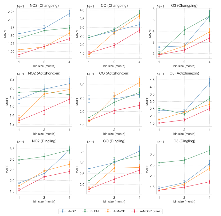
Figure 3: MAPE and standard errors for the prediction of fine-grained aggregated time-series datasets. Each row shows the results for each of the monitoring stations, and each column shows the results for each of the pollutants.

6.3 Baselines

We compared A-MoGP with Gaussian process regression for binned data [35]. This model is a special case of A-MoGP when only target aggregate dataset in a single domain is available; in this article, we call it aggregated Gaussian process (A-GP) with single-output. Another baseline is one of the standard MoGP models, semiparametric latent factor model (SLFM) [17]. A-MoGP is an extension of SLFM; A-MoGP newly incorporates the observation model with aggregation processes for handling aggregate data. SLFM assumes that samples are observed at location points rather than supports; we thus associate each attribute value with the centroid of the support. Additionally, A-GP and SLFM do not have a mechanism for knowledge transfer across domains.

6.4 Results for time-series data

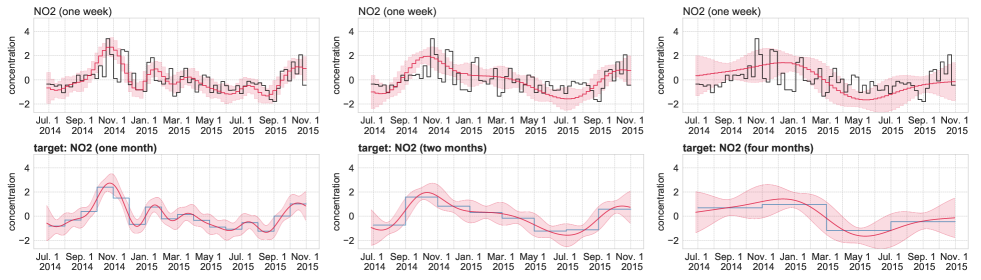
Figure 4: Prediction result of A-GP for the attributes in Aotizhongxin. In the first row, the black and red lines are the true and predicted values, respectively; the red shaded area denotes twice the standard deviation in prediction at each fine-grained bin. The blue and red lines in the second row are the training data and its prediction, respectively; the predictive variance is calculated on a continuous timeline.

Figure 5: Prediction result of SLFM for the attributes in Aotizhongxin. Further figure details are the same as Figure 4.

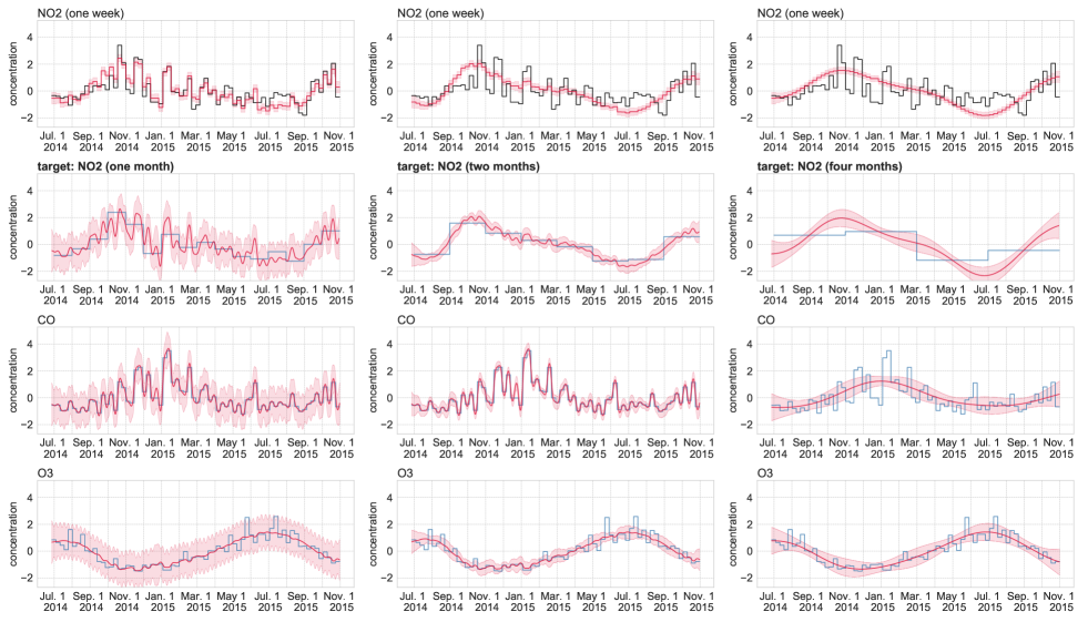
Figure 6: Prediction result of A-MoGP for the attributes in Aotizhongxin. Further figure details are the same as Figure 4.

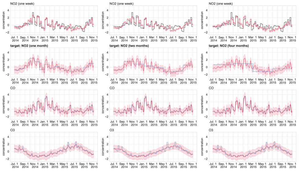
Figure 7: Prediction result of A-MoGP (trans) for the attributes in Aotizhongxin. Further figure details are the same as Figure 4.

(a) Relationships estimated by A-MoGP.

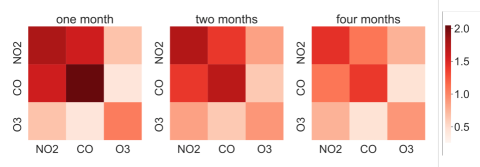
(b) Relationships estimated by A-MoGP (trans).

Figure 8: Estimated relationships between attributes when using NO2 in Aotizhongxin as the target dataset.

In this section, we present the experimental results for time-series data of air pollutants. Figure 3 shows MAPE and standard errors for A-GP, SLFM, A-MoGP, and A-MoGP (trans). Here, A-GP, SLFM, and A-MoGP were trained and tested using the aggregate datasets from a single domain; A-MoGP (trans) utilized all the datasets from three domains. As expected, one observes that for all models, MAPE increased with the bin size for creating the coarse-grained target dataset. In many cases, A-MoGP achieved better performance than A-GP and SLFM. This result shows that A-MoGP can effectively utilize multiple aggregate datasets from a single domain. Moreover, A-MoGP (trans) outperformed A-MoGP, especially when the bin size was set to two and four months. This result shows that the refinement performance can be improved by making use of aggregate datasets from other domains even if the target dataset is coarser.

TABLE III: MAPE and standard errors for the prediction of fine-grained areal data in New York City and Chicago. The numbers in parentheses denote the number $L$ of the latent GPs estimated by the leave-one-out cross-validation.

	A-GP	SLFM	A-MoGP	A-MoGP (trans)
Poverty rate	0.263 $\pm$ 0.032 (–)	0.184 $\pm$ 0.019 (2)	0.186 $\pm$ 0.018 (3)	0.168 $\pm$ 0.018 (3)
Unemployment rate	0.215 $\pm$ 0.023 (–)	0.172 $\pm$ 0.020 (6)	0.177 $\pm$ 0.021 (7)	0.151 $\pm$ 0.020 (6)
PM2.5	0.054 $\pm$ 0.007 (–)	0.037 $\pm$ 0.005 (3)	0.037 $\pm$ 0.006 (3)	0.039 $\pm$ 0.007 (4)
Mean commute	0.072 $\pm$ 0.009 (–)	0.072 $\pm$ 0.009 (6)	0.054 $\pm$ 0.006 (3)	0.051 $\pm$ 0.006 (4)
Recycle diversion rate	0.282 $\pm$ 0.037 (–)	0.257 $\pm$ 0.029 (4)	0.180 $\pm$ 0.022 (2)	0.166 $\pm$ 0.021 (4)
Population density	0.354 $\pm$ 0.039 (–)	0.386 $\pm$ 0.046 (4)	0.355 $\pm$ 0.040 (3)	0.325 $\pm$ 0.052 (4)
Crime rate	0.601 $\pm$ 0.129 (–)	0.472 $\pm$ 0.081 (3)	0.427 $\pm$ 0.105 (2)	0.426 $\pm$ 0.124 (8)

(a) New York City

	A-GP	SLFM	A-MoGP	A-MoGP (trans)
Poverty rate	0.255 $\pm$ 0.031 (–)	0.309 $\pm$ 0.030 (2)	0.243 $\pm$ 0.031 (3)	0.223 $\pm$ 0.021 (7)
Unemployment rate	0.414 $\pm$ 0.073 (–)	0.356 $\pm$ 0.049 (2)	0.240 $\pm$ 0.025 (3)	0.268 $\pm$ 0.037 (8)

(b) Chicago

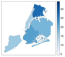
(a) Training data (coarse granularity)

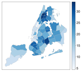
(b) True data (fine granularity)

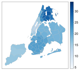
(c) A-GP

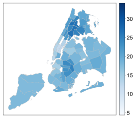
(d) SLFM

(e) A-MoGP

(f) A-MoGP (trans)

Figure 10: Refinement results of the Poverty rate dataset in New York City.

Figures 4, 5, 6, and 7 illustrate the prediction results of the attributes in Aotizhongxin, by A-GP, SLFM, A-MoGP, and A-MoGP (trans), respectively. Here, the target dataset is set to NO2 in Aotizhongxin. In these figures, the first row is the result for the test dataset (i.e., fine-grained target dataset). The remaining rows in these figures are the results for the training datasets, including the coarse-grained target dataset. In the results of A-GP, A-MoGP, and A-MoGP (trans), the predictive variance (depicted by the red shaded area) was obtained via the double integral of the posterior covariance function $\hat{{\bf K}}_{v^{\prime}}^{*}(\bm{x},\bm{x}^{\prime})$ (24) over the corresponding bin. Each column in these figures shows the result when using the coarse-grained target dataset with the corresponding bin size (described by the bold font in the figures). As one can see from Figure 4, A-GP incorporating the aggregation process can effectively interpolate the target aggregated attribute without over-fitting while encouraging consistency between the coarse- and the fine-grained target dataset. However, the performance of A-GP is limited because it does not use multiple datasets to refine the coarse-grained target dataset. Although SLFM can utilize multiple datasets from a single domain, it does not have the observation model for handling aggregate datasets; this might prevent the model from learning properly. In the third column of Figure 5, one observes the over-fitting of SLFM to the CO dataset because SLFM regarded the areal data as the point-referenced data. It is one of the reasons why SLFM does not yield better performance in refining the coarse-grained dataset. As one can see from Figure 6, A-MoGP captured the fine-scale variation of the target attribute by utilizing the relevant attribute (i.e., CO), only in the case where the target dataset has the relatively fine granularities (i.e., one month). In Figure 7, one can see that A-MoGP (trans) yielded an excellent prediction even if there is only the target dataset with coarser granularities. By comparing the estimated function (depicted by the red lines in Figures 4, 5, 6, and 7) when setting the target coarse-grained bin size to four months among all the models, we can see that the improvement with A-MoGP (trans) is obvious. This is because A-MoGP (trans) can utilize the aggregate datasets in multiple domains and appropriately learn the relationships between attributes and the covariances of data points. To confirm this observation, in Figure 8, we show the visualization of the relationships between attributes, estimated by A-MoGP and A-MoGP (trans). Letting $\bar{{\bf W}}^{\prime}_{v}$ be an $|\mathcal{S}_{v}|\times|\mathcal{L}|$ matrix whose $(s,l)$-entry is the variational posterior mean $\bar{w}_{vsl}^{\prime}$ in (15), the relationships between attributes were calculated as follows: $\bar{{\bf W}}^{\prime}_{v}\bar{{\bf W}}^{\prime\top}_{v}\in\mathbb{R}^{|\mathcal{S}_{v}|\times|\mathcal{S}_{v}|}$, which is known as a coregionalization matrix [15]. Figure 8 illustrates the absolute values of the elements of the coregionalization matrix. This result shows that A-MoGP captured the useful relationship between attributes, that is, the correlation between NO2 and CO, only in the case where the bin size for the coarse-grained target attribute was one month. Meanwhile, A-MoGP (trans) emphasized this relationship even if the target attribute was associated with coarser time bins.

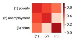
(a) Estimated relationships (Chicago).

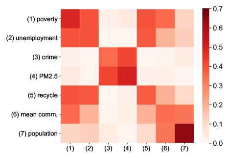
(b) Estimated relationships (New York City).

Figure 11: Relationships between attributes learned by A-MoGP (trans). The target dataset was set to the Poverty rate dataset in New York City.

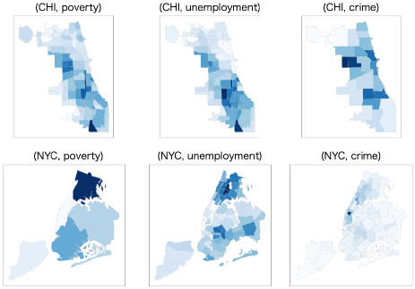
Figure 12: Visualizations of the training datasets contained in both Chicago and New York City.

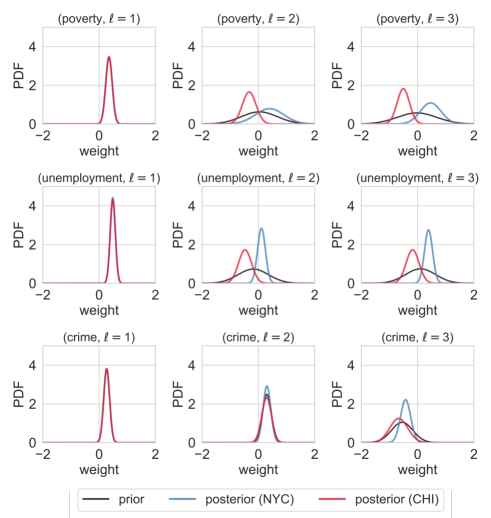
Figure 13: Visualizations of the prior and the variational posterior for weight parameters, estimated by A-MoGP (trans).

6.5 Results for areal data

This section presents the experimental results for areal datasets in cities. Table III shows MAPE and standard errors for A-GP, SLFM, A-MoGP, and A-MoGP (trans). Here, the experiments for the Crime rate dataset in Chicago have not been conducted because the coarser version for training is not available online. For all datasets, A-MoGP and A-MoGP (trans) achieved better performance in refining the coarse-grained areal dataset than the baseline models. Also, in most cases, A-MoGP (trans) was able to use the aggregate datasets in two cities to improve refinement performance. Figure 10 shows the Poverty rate dataset in New York City and the refinement results attained by A-GP, SLFM, A-MoGP, and A-MoGP (trans). Compared with the true values in Figure 10(b), A-MoGP (trans) yielded more accurate estimates of the fine-grained data than the other models.

We analyzed the relationships between the attributes, estimated by A-MoGP (trans). Figure 11 shows the visualization of the relationships when setting the Poverty rate dataset in New York City as the target dataset, which was illustrated by the same procedure as that described in Section 6.4. In Figure 11, one can see that the poverty rate and the unemployment rate had strong relationships in both cities; meanwhile, the strength of the relationship between the poverty rate and the crime rate was stronger in Chicago than that in New York City. Comparing these results with the visualizations of training datasets in Figure 12, we can confirm that A-MoGP (trans) captures the correlations between three attributes (i.e., poverty rate, unemployment rate, and crime rate) appropriately. One advantage of A-MoGP (trans) is that it has the mechanism for knowledge transfer across domains, allowing for utilizing datasets from multiple domains to learn weight parameters defining relationships between attributes. Sharing the prior distribution (6) for the weight parameters among all domains makes the knowledge transfer possible; Figure 13 visualizes the prior (6) and the variational posterior (15), estimated by A-MoGP (trans). Each tile shows the distribution for the weight $w_{vsl}$ of the $l$-th latent GP in each attribute. One observes that the prior variances were small in the case of $l=1$ and in the case of the Crime rate dataset of $l=2$ (see black lines in Figure 13); the variational posteriors for New York City (blue lines in Figure 13) and Chicago (red lines in Figure 13) were close to the prior distributions. In these cases, knowledge transfer is more encouraged. Accordingly, Table III and Figure 13 show that A-MoGP (trans) achieves performance improvement by using the aggregate datasets from both cities via the knowledge transfer.

7 Conclusion

In this article, we have proposed the Aggregated Multi-output Gaussian Process (A-MoGP) that can estimate functions for attributes by utilizing aggregate datasets of respective granularities from multiple domains. Experiments on real-world datasets have confirmed that the A-MoGP can perform better than baselines in refining coarse-grained aggregate data; moreover, the A-MoGP has improved performance by using aggregate datasets from multiple domains via the knowledge transfer across domains.

There are several research directions that can be explored in the future. First, we can introduce alternative likelihoods such as the Poisson distribution for count data. Second, we can speed up the inference using the inducing point technique, similarly to [51]. Third, incorporating rich additional data is promising to improve refinement performance. For example, satellite images are known to be helpful in the refinement of spatially aggregated data [36]. A powerful option to leverage such data is to use deep neural networks as a model component, which would help automatically extract meaningful representations from data.

References

- [1] A. Rupasinghaa and S. J. Goetz, “Social and political forces as determinants of poverty: A spatial analysis,” The Journal of Socio-Economics, vol. 36, no. 4, pp. 650–671, 2007.
- [2] C. C. Smith, A. Mashhadi, and L. Capra, “Poverty on the cheap: Estimating poverty maps using aggregated mobile communication networks,” in CHI, 2014, pp. 511–520.
- [3] A. Bogomolov, B. Lepri, J. Staiano, N. Oliver, F. Pianesi, and A. Pentland, “Once upon a crime: Towards crime prediction from demographics and mobile data,” in ICMI, 2014, pp. 427–434.
- [4] H. Wang, D. Kifer, C. Graif, and Z. Li, “Crime rate inference with big data,” in KDD, 2016, pp. 635–644.
- [5] P. Keil, J. Belmaker, A. M. Wilson, P. Unitt, and W. Jetz, “Downscaling of species distribution models: A hierarchical approach,” Methods in Ecology and Evolution, vol. 4, no. 1, pp. 82–94, 2013.
- [6] R. Howitt and A. Reynaud, “Spatial disaggregation of agricultural production data using maximum entropy,” European Review of Agricultural Economics, vol. 30, no. 2, pp. 359–387, 2003.
- [7] A. Xavier, M. B. C. Freitas, M. D. S. Rosrio, and R. Fragoso, “Disaggregating statistical data at the field level: An entropy approach,” Spatial Statistics, vol. 23, pp. 91–103, 2016.
- [8] H. J. W. Sturrock, J. M. Cohen, P. Keil, A. J. Tatem, A. L. Menach, N. E. Ntshalintshali, M. S. Hsiang, and R. D. Gosling, “Fine-scale malaria risk mapping from routine aggregated case data,” Malaria Journal, vol. 13, p. 421, 2014.
- [9] R. L. Wilby, S. P. Zorita, E. Timbal, B. Whetton, and L. O. Mearns, Guidelines for Use of Climate Scenarios Developed from Statistical Downscaling Methods, 2004. [Online]. Available: http://www.narccap.ucar.edu/doc/tgica-guidance-2004.pdf
- [10] E. Zorita and H. von Storch, “The analog method as a simple statistical downscaling technique: Comparison with more complicated methods,” Journal of Climate, vol. 12, pp. 2474–2489, 1999.
- [11] M. Jerrett, R. T. Burnett, B. S. Beckerman, M. C. Turner, D. Krewski, G. Thurston, and et al., “Spatial analysis of air pollution and mortality in California,” American Journal of Respiratory and Critical Care Medicine, vol. 188, no. 5, pp. 593–599, 2013.
- [12] Y. Tanaka, T. Iwata, T. Kurashima, H. Toda, N. Ueda, and T. Tanaka, “Time-delayed collective flow diffusion models for inferring latent people flow from aggregated data at limited locations,” Artificial Intelligence, vol. 292, p. 103430, 2021.
- [13] F. Yousefi, M. T. Smith, and M. A. Álvarez, “Multi-task learning for aggregated data using Gaussian processes,” in NeurIPS, 2019.
- [14] C. E. Rasmussen and C. K. I. Williams, Gaussian Processes for Machine Learning. MIT Press, 2006.
- [15] M. A. Álvarez, L. Rosasco, and N. D. Lawrence, “Kernels for vector-valued functions: A review,” Foundations and Trends® in Machine Learning, vol. 4, no. 3, pp. 195–266, 2012. [Online]. Available: http://dx.doi.org/10.1561/2200000036
- [16] E. Bonilla, K. M. Chai, and C. Williams, “Multi-task Gaussian process prediction,” in NeurIPS, 2008, pp. 153–160.
- [17] Y. W. Teh, M. Seeger, and M. I. Jordan, “Semiparametric latent factor models,” in AISTATS, 2005, pp. 333–340.
- [18] P. Boyle and M. Frean, “Dependent Gaussian processes,” in NeurIPS, 2005, pp. 217–224.
- [19] T. V. Nguyen and E. V. Bonilla, “Collaborative multi-output Gaussian processes,” in UAI, 2014, pp. 643–652.
- [20] K. Yu, V. Tresp, and A. Schwaighofer, “Learning Gaussian processes from multiple tasks,” in ICML, 2005, pp. 1012–1019.
- [21] C. A. Micchelli and M. Pontil, “Kernels for multi-task learning,” in NeurIPS, 2004, pp. 921–928.
- [22] D. Higdon, “Space and space-time modelling using process convolutions,” Quantitative Methods for Current Environmental Issues, pp. 37–56, 2002.
- [23] J. Luttinen and A. Ilin, “Variational Gaussian-process factor analysis for modeling spatio-temporal data,” in NeurIPS, 2009, pp. 1177–1185.
- [24] D. Kingma and M. Welling, “Auto-encoding variational Bayes,” in ICLR, 2014.
- [25] Y. Tanaka, T. Tanaka, T. Iwata, T. Kurashima, M. Okawa, Y. Akagi, and H. Toda, “Spatially aggregated Gaussian processes with multivariate areal outputs,” in NeurIPS, 2019.
- [26] C. A. Gotway and L. J. Young, “Combining incompatible spatial data,” Journal of the American Statistical Association, vol. 97, no. 458, pp. 632–648, 2002.
- [27] W. S. Robinson, “Ecological correlations and the behavior of individuals,” Americal Sociological Review, vol. 15, pp. 351–357, 1950.
- [28] G. King, A solution to the ecological inference problem: Reconstructing individual behavior from aggregate data. Princeton University Press, 2013.
- [29] N. W. Park, “Spatial downscaling of TRMM precipitation using geostatistics and fine scale environmental variables,” Advances in Meteorology, vol. 2013, pp. 1–9, 2013.
- [30] D. Murakami and M. Tsutsumi, “A new areal interpolation technique based on spatial econometrics,” Procedia-Social and Behavioral Sciences, vol. 21, pp. 230–239, 2011.
- [31] B. M. Taylor, R. Andrade-Pacheco, and H. J. W. Sturrock, “Continuous inference for aggregated point process data,” Journal of the Royal Statistical Society: Series A (Statistics in Society), p. 12347, 2018.
- [32] K. Wilson and J. Wakefield, “Pointless spatial modeling,” Biostatistics, vol. 21, no. 2, pp. e17–e32, 2018.
- [33] T. M. Burgess and R. Webster, “Optimal interpolation and isarithmic mapping of soil properties I: The semi-variogram and punctual kriging,” Journal of Soil Science, vol. 31, no. 2, pp. 315–331, 1980.
- [34] R. Murray-Smith and B. A. Pearlmutter, “Transformations of Gaussian process priors,” in DSMML, 2004, pp. 110–123.
- [35] M. T. Smith, M. A. Álvarez, and N. D. Lawrence, “Gaussian process regression for binned data,” in arXiv e-prints, arXiv:1809.02010v2 [stat.ML], 2018.
- [36] H. C. L. Law, D. Sejdinovic, E. Cameron, T. C. D. Lucas, S. Flaxman, K. Battle, and K. Fukumizu, “Variational learning on aggregate outputs with Gaussian processes,” in NeurIPS, 2018, pp. 6084–6094.
- [37] Y. Tanaka, T. Iwata, T. Tanaka, T. Kurashima, M. Okawa, and H. Toda, “Refining coarse-grained spatial data using auxiliary spatial data sets with various granularities,” in AAAI, 2019, pp. 5091–5100.
- [38] Y. Zhang, N. Charoenphakdee, Z. Wu, and M. Sugiyama, “Learning from aggregate observations,” in NeurIPS, 2020, pp. 7993–8005.
- [39] S. L. Chau, S. Bouabid, and D. Sejdinovic, “Deconditional downscaling with Gaussian processes,” in NeurIPS, 2021, pp. 17 813–17 825.
- [40] D. E. Myers, “Matrix formulation of co-kriging,” Journal of the International Association for Mathematical Geology, vol. 14, no. 3, pp. 249–257, 1982.
- [41] P. Goovaerts, Geostatistics For Natural Resources Evaluation. Oxford University Press, 1997.
- [42] A. G. Journel and C. J. Huijbregts, Mining Geostatistics. Academic Press, 1978.
- [43] O. Hamelijnck, T. Damoulas, K. Wang, and M. Girolami, “Multi-resolution multi-task Gaussian processes,” in NeurIPS, 2019.
- [44] Y. Tanaka, Probabilistic Models for Spatially Aggregated Data. Doctoral Thesis, Graduate School of Informatics, Kyoto University, 2019.
- [45] C. M. Bishop, Pattern Recognition and Machine Learning. Springer, 2006.
- [46] S. Zhang, B. Guo, A. Dong, J. He, Z. Xu, and S. Chen, “Cautionary tales on air-quality improvement in Beijing,” in Proceedings of the Royal Society A, vol. 473, no. 2005, 2017, p. 20170457.
- [47] City of New York, “NYC open data,” https://opendata.cityofnewyork.us/.
- [48] City of Chicago, “Chicago Data Portal,” https://data.cityofchicago.org/.
- [49] D. P. Kingma and J. Ba, “Adam: A method for stochastic optimization,” in ICLR, 2015. [Online]. Available: http://arxiv.org/abs/1412.6980
- [50] A. Paszke, S. Gross, F. Massa, A. Lerer, J. Bradbury, G. Chanan, T. Killeen, Z. Lin, N. Gimelshein, L. Antiga, A. Desmaison, A. Kopf, E. Yang, Z. DeVito, M. Raison, A. Tejani, S. Chilamkurthy, B. Steiner, L. Fang, J. Bai, and S. Chintala, “Pytorch: An imperative style, high-performance deep learning library,” in NeurIPS, 2019, pp. 8024–8035.
- [51] M. Titsias, “Variational learning of inducing variables in sparse Gaussian processes,” in AISTATS, 2009, pp. 567–574.