Scalable Multiple Network Inference With The Joint Graphical Horseshoe
MRC Biostatistics Unit
University of Cambridge
camilla.lingjaerde@mrc-bsu.cam.ac.uk
&
MRC Weatherall Institute for Molecular Medicine
University of Oxford
benjamin.fairfax@oncology.ox.ac.uk
&
MRC Biostatistics Unit
University of Cambridge
sylvia.richardson@mrc-bsu.cam.ac.uk
&
MRC Biostatistics Unit
University of Cambridge
helene.ruffieux@mrc-bsu.cam.ac.uk
Abstract
Network models are useful tools for modelling complex associations. In statistical omics, such models are increasingly popular for identifying and assessing functional relationships and pathways. If a Gaussian graphical model is assumed, conditional independence is determined by the non-zero entries of the inverse covariance (precision) matrix of the data. The Bayesian graphical horseshoe estimator provides a robust and flexible framework for precision matrix inference, as it introduces local, edge-specific parameters which prevent over-shrinkage of non-zero off-diagonal elements. However, its applicability is currently limited in statistical omics settings, which often involve high-dimensional data from multiple conditions that might share common structures. We propose (i) a scalable expectation conditional maximisation (ECM) algorithm for obtaining a posterior estimate of the precision matrix in the graphical horseshoe, and (ii) a novel joint graphical horseshoe estimator, which borrows information across multiple related networks to improve estimation. We show numerically that our single-network ECM approach is more scalable than the existing graphical horseshoe Gibbs implementation, while achieving the same level of accuracy. We also show that our joint-network proposal successfully leverages shared edge-specific information between networks while still retaining differences, outperforming state-of-the-art methods at any level of network similarity. Finally, we leverage our approach to clarify gene regulation activity within and across immune stimulation conditions in monocytes, and formulate hypotheses on the pathogenesis of immune-mediated diseases.
Keywords Bayesian graphical models Cancer genomics Expectation conditional maximisation Gene networks Genomics Graphical horseshoe Horseshoe prior High-dimensional inference Integrative analysis Multi omics Network models
1 Introduction
In statistical omics, network models are increasingly popular for representing complex associations and assessing pathway activity. With such models, the links between genes, proteins or other types of omics data can be represented and studied, providing valuable insight into functional relationships. The progress of high-throughput genomic technologies has led to the collection of large, genome-wide data sets, and the availability of biomeasurements of different types has enabled the development of integrative modelling approaches which can increase statistical power while providing detailed insight into complex biological mechanisms (Someren et al. (2002); Karczewski and Snyder (2018)).
If a Gaussian graphical model is assumed, an association (conditional independence) network can be estimated by determining the non-zero entries of the inverse covariance (precision) matrix of the data. There is significant literature on this problem, both frequentist and Bayesian. Notable frequentist methods include the neighbourhood selection (Meinshausen and Bühlmann (2006)), the graphical lasso (Friedman et al. (2008)) and the graphical SCAD (Fan et al. (2009)). In later years, Bayesian methods such as the Bayesian graphical lasso (Wang et al. (2012)), Bayesian spike-and-slab approaches (Wang (2015)) and the graphical horseshoe (Li et al. (2019a)) have gained popularity. The Bayesian model formulation of the graphical horseshoe leads to many desirable properties, particularly for identifying weak edges. Indeed, the global-local horseshoe prior it relies on permits the introduction of edge-specific parameters that prevent over-shrinkage of non-zero off-diagonal elements, resulting in a highly flexible framework. However, in the high-dimensional settings commonly needed for investigating biological networks, the Gibbs sampling implementation proposed by Li et al. (2019a) becomes computationally inefficient or even unfeasible. Moreover, the graphical horseshoe has only been formulated for a single network, whereas interest has grown in the network analysis of multiple data sets that might share common structures. In biomedical applications, such related data sets could be different tissues, conditions or patient subgroups, or different omics types, such as gene levels and the protein levels encoded by these genes. A joint approach that utilises the common information while preserving the differences will both have increased statistical power and provide insight into the different mechanisms in play.
In the field of multiple Gaussian graphical models, notable frequentist methods include the joint graphical lasso (Danaher et al. (2014)), which enforces similar graphical structures by solving a penalised likelihood problem, and a group extension of the graphical lasso to multiple networks (Guo et al. (2011)). In a Bayesian framework, Peterson et al. (2015) propose a Gibbs sampling approach which uses a Markov random field prior on multiple graphs to learn the similarity of graphical structures. Other notable Bayesian approaches include two expectation-maximisation (EM) approaches, namely, the Bayesian spike-and-slab joint graphical lasso (Li et al. (2019b)), which builds on seminal work by Wang (2015) and formulates a multiple-network model based on a Gaussian spike-and-slab prior, and GemBag (Yang et al. (2021)), which relies on a spike-and-slab prior with Laplace distributions. For a more thorough review on existing Bayesian graphical methods, we refer to Ni et al. (2022).
The method presented in this paper is, to our knowledge, the first to adapt graphical modelling based on global-local priors to the multiple network setting. We propose an expectation conditional maximisation (ECM) algorithm for obtaining a posterior estimate of the precision matrix in the graphical horseshoe which allows us to tackle network inference in biological problems of realistic sizes. Building on this efficient implementation, we formulate a joint model that permits borrowing information between multiple networks using the graphical horseshoe prior. We provide the two R packages fastGHS and jointGHS, which implement the single and joint methods respectively.
The paper is organised as follows. In Section 2, we recall the classical graphical horseshoe estimator of Li et al. (2019a) and discuss the advantages of the horseshoe prior in graphical settings. In Section 3, we motivate the need for further development to enable practical and meaningful inference at scale by introducing a multi-condition gene regulation study in monocytes. In Section 4, we describe our new inference procedure for the single-network graphical horseshoe, and in Section 5, we present our joint graphical horseshoe model formulation. In Section 6, we demonstrate the performance of our proposed methodology on simulated data, and in Section 7, we apply it to the monocyte gene regulation study. Finally, we highlight possible extensions in Section 8.
2 Problem statement
Consider a network model where each node is associated with some measurable attribute. Observed values of the multivariate random vector of node attributes, each entry corresponding to one of variables, can then be used to infer a graph under suitable model assumptions. Given multivariate Gaussian node attributes, with observation matrix with i.i.d. rows , we can infer a partial correlation network by estimating the inverse covariance matrix, or precision matrix, . The partial correlation between nodes and conditioned upon all others is then given by
where the ’s are the entries of and is the set of all node pairs (Lauritzen (1996)). For Gaussian variables, correlation equal to zero is equivalent to independence, which implies that a conditional independence graph can be constructed by determining the non-zero entries of the precision matrix. The graph is assumed to be sparse, i.e., the number of edges in the edge set relative to the number of potential edges in the graph, , is small. The precision matrix must also necessarily be positive definite, .
Li et al. (2019a) have recently proposed the graphical horseshoe to obtain a sparse estimate of the precision matrix , repurposing the horseshoe prior initially introduced by Carvalho et al. (2010) in the normal means setting to a graphical setting. The graphical horseshoe model puts horseshoe priors on the off-diagonal elements of the precision matrix, encouraging sparse solutions. An uninformative prior is put on the diagonal elements, and the positive definiteness constraint is respected. Due to symmetry, it is sufficient to consider the upper off-diagonal elements of . Normal scale mixtures with half-Cauchy hyperpriors are used on the off-diagonal elements. The hierarchy of the model is as follows:
| (1) | ||||
with and where is the half-Cauchy distribution with density . A key feature of the horseshoe prior in (2) is the presence of local shrinkage parameters, , which are meant to flexibly capture edge-specific effects with no or very limited over-shrinkage, while the global parameter is set to ensure overall sparsity. In the next section, we motivate the extension of the graphical horseshoe to a multiple network setting, with a scalable implementation.
3 Data and motivating example
A wide array of prevalent diseases, such as inflammatory bowel disease, rheumatoid arthritis and cancer, are believed to result from an inappropriate immune activity and consequent inflammation. It is now established that exposing monocyte cell cultures to specific stimuli can create conditions that resemble certain immune-mediated disease states (Biswas and Mantovani (2010)). Indeed, different stimuli may activate different cellular or molecular pathways that contribute to disease development. Hence, systematically investigating the impact of different types of immune stimulation on gene regulatory activity – and pinpointing the mechanisms that are common to several stimuli or stimulus specific – can provide valuable insights into the pathophysiology of such diseases.
We propose to contribute to this research by analysing graphical structures from a detailed gene expression dataset where primary CD14+ monocytes in healthy European individuals were exposed to different types of immune stimulation (hereafter “conditions”). Specifically, monocyte expression was quantified using Illumina HumanHT-12 v4 BeadChip arrays before and after immune stimulation via exposition to inflammation proxies, namely, () or differing durations of lipopolysaccharide (LPS 2h or LPS 24h). The number of samples available in each condition is , , , for unstimulated cells, and -, LPS 2h- and LPS 24h- stimulated cells, respectively (Fairfax et al. (2014)).
Examining the effect of genetic variation on gene regulatory activity after stimulation can help pinpointing gene sets implicated in disease risk and development. Indeed, previous studies suggest that gene stimulation triggers regulatory activity that leads to a beneficial environment for hotspots to establish (Fairfax et al. (2014); Lee et al. (2014); Kim et al. (2014); Ruffieux et al. (2020)) – hotspots are genetic variants regulating large numbers of genes, thereby potentially representing important players in disease mechanisms (Yao et al. (2017)). We will therefore focus our study to networks of genes under hotspot control, in the different conditions.
While Fairfax et al. (2014) mainly report condition-specific gene regulatory activities, they also observe effects across all conditions. The largest hotspot identified by Ruffieux et al. (2020) is persistent across all four conditions. Specifically, using their global-local hotspot modelling approach ATLASQTL, they found that the genetic variant rs6581889 was the top hotspot in the , unstimulated and LPS 2h studies (associated with , and transcripts, respectively), and it was the second largest hotspot in the LPS 24h study (associated with transcripts). This hotspot is located on chromosome 12, only a few Kb away from two genes it controls, namely, LYZ and YEATS4, which are thought to play a central role in the pathogenesis of immune disorders (Fairfax et al. (2012)).
Given the shared hotspot control in all four immune stimulation conditions, borrowing information with a joint network approach on the controlled genes across these conditions seems particularly appropriate to further investigate the gene regulation mechanisms triggered by rs6581889. At the same time, Ruffieux et al. (2020) found that there is only a partial overlap between the genes associated with the hotspot across the different conditions, which calls for a modelling approach that can also effectively detect stimulus-specific effects – such effects being highly relevant to understand how distinct pathways may be activated in different disease states. Such an analysis should help characterising the complex interplays among the genes controlled, i.e., the direct effects on the distal genes or the indirect effects, mediated via other genes controlled by the hotspot (typically via proximal genes, such as LYZ and YEATS4). Although graphical modelling approaches seem particularly appropriate to disentangle direct and mediated effects, they have not been employed thus far.
With its desirable theoretical properties as well as its high performance in numerical studies, the graphical horseshoe estimator (Li et al. (2019a)) would be a natural choice for graph inference. However its applicability in the above monocyte setting is hampered by two limitations: first, its Gibbs sampler implementation does not scale to the problem dimensions ( genes for observations in each condition). Second, its model is formulated for the analysis of a single network, meaning that it can only be applied separately to each of the four conditions. Although relevant for identifying common structures across the conditions, the Bayesian spike-and-slab joint graphical lasso (Li et al. (2019b)) and the joint graphical lasso (Danaher et al. (2014)) do not enjoy the flexibility granted by the horseshoe prior’s local scales for identifying network-specific effects (whose detection is key to disentangle disease-specific mechanisms as explained above). Moreover, these methods did not reach convergence within hours, as jointly modelling all four conditions requires inferring a total of edges. This severe high dimensionality makes essential to develop approaches that are specifically designed to scale to the current statistical omics problem sizes.
Motivated by the monocyte problem, this work is concerned with proposing a new framework that addresses the two shortcomings outlined above to enable effective network inference in realistic practical settings. Namely, we aim to (i) develop an expectation conditional maximisation (ECM) algorithm for the graphical horseshoe as a fast yet accurate alternative to the Gibbs sampling procedure proposed by Li et al. (2019a), and (ii) formulate a joint model for multiple networks, leveraging the global-local horseshoe feature to borrow strength across shared patterns while preserving differences across networks.
Equipped with this framework, we will return to the monocyte problem in Section 7 to demonstrate the computational feasibility of joint network modelling on these data and exploit the advantages of the global-local formulation for inferring and interpreting condition-specific and shared gene regulation structures.
4 An ECM algorithm for estimating the graphical horseshoe
As a first step in detailing our proposal, we outline the expectation conditional maximisation (ECM) procedure, which adapts the spike-and-slab EM approach of Ročková and George (2014) to the graphical horseshoe setting. We first detail the updates for the single-network graphical horseshoe prior (2). The ECM approach, described first by Meng and Rubin (1993), is a generalised EM algorithm (Dempster et al. (1977)) where a complex maximisation step (M-step) is replaced with several computationally simpler conditional maximisation steps (CM-steps).
4.1 Full conditional posteriors
As in Li et al. (2019a), the full conditional posteriors of the local ’s can be derived by introducing the augmented variables . We next employ the following reparameterisation, introducing the latent and writing
Using a key observation from Makalic and Schmidt (2015), we find the full conditional posteriors as
| (2) |
where denotes all other variables. The latent variables can be collected in the latent matrix . The global shrinkage parameter in (2) is for now treated as a fixed hyperparameter; its specification will be detailed in Section 5.3. To obtain conditional posteriors for the precision matrix and the local scale parameters, each column and row of the matrices and are partitioned from a matrix of parameters. Without loss of generality, we describe the updates for the last row and column. As in Wang et al. (2012), we write
where is the scatter matrix of the observed data . The diagonal elements of are not of relevance and can be set to an arbitrary value such as . The posterior distribution for the last column (and row) of can be obtained as
With a variable change, the conditional distributions can be reformulated as
| (3) |
where and . By iteratively permuting each row and column to be the last, the conditional posterior of all elements of the precision matrix can then be found row and column wise.
4.2 ECM algorithm
Given the estimates from the previous iteration , the objective function is obtained as
| (4) | ||||
where denotes and const. is a constant not depending on or . Note that the objective function accounts for the full priors of and .
In the E-step of the algorithm, the conditional expectations in (4.2) are computed, and the CM-step performs the maximisation with respect to . Similarly to the Bayesian spike-and-slab joint graphical lasso of Li et al. (2019b) where the objective function is maximised over both the precision matrix and sparsity parameters, this approach finds the posterior mode of , accounting for prior distributions on all parameters.
From (4.1), the full conditional distributions of the ’s are inverse Gamma. Therefore, the E-step updates are:
| (5) |
where is the digamma function.
Next, the CM-step maximises (4.2) with respect to in a coordinate ascent fashion, with the expectations replaced with the expressions found in (4.2). The following closed-form updates are obtained for the ’s
| (6) |
There is no closed form for the update of the precision matrix, however, (4.1) gives the updates for the last row and column of :
| (7) |
setting at each iteration. By iteratively permuting each row and column to be the last, all elements of the precision matrix can be updated row and column wise. With these updates, the positive definiteness constraint for is maintained at each iteration as long as the initial value is positive definite. This can be shown with an argument equivalent to that of Wang et al. (2012): assume that the update is positive definite, then all its leading principal minors are positive. After updating the last row and column as in (4.2), the updated precision matrix has the same leading principal minors as in except for the last one, which is of order . The last leading principal minor is clearly equal to , where is the leading principal minor of and thus positive, and we have, from (4.1), that . Consequently, and so the updated is positive definite.
With this CM-step update, it is ensured that (Meng and Rubin (1993)). By iterating between the E-step and the CM-step until convergence, we obtain an estimator of the posterior mode of . The full derivations for this section are given in Section S.1 of Supplement A.
One of the main computational advantages of the ECM approach over stochastic search is that the posterior mode is fast to obtain. The estimates are computed directly and a full stochastic search is not necessary. Further, the entries corresponding to unidentified edges tend to converge to values close to zero and the separation with the identified edges increases as the algorithm converges – such an observation has also been reported by others in the context of EM or variational inference (Kook et al. (2021)). We hereafter refer to this ECM implementation as “fastGHS”.
5 Multiple network inference
In this section, we describe the joint graphical horseshoe for multiple network inference. By sharing information through common latent variables, the method gives more precise estimates for networks with any level of similarity. The heavy tails of the horseshoe prior permits effectively capturing network-specific edges, a property that few Bayesian methods developed for similar purposes share. The resulting joint graphical horseshoe estimator simultaneously shares information between networks and captures their differences. In addition, due to the scalability of the ECM implementation, our method allows for joint network modelling for a larger number of networks than existing Bayesian approaches do.
5.1 Joint graphical horseshoe model formulation
Given networks with nodes each, and observation matrices for , we are interested in estimating the precision matrices . We let the precision matrix follow the hierarchical model
with , . This is the standard graphical horseshoe model for each network separately. To share information across networks, we introduce the latent variables and write
We then derive the full conditional posteriors. Because the ’s of the different data sets are independent given the ’s, we have
similarly to the standard graphical horseshoe. Hence, information is now shared across networks through the common latent variable , and the full conditional posterior of the ’s now depends on the ’s of all networks:
| (8) |
The derivation of (8) is given in Section S.1.4 of Supplement A.
The global scales are network-specific to allow for different sparsity levels across networks; their specification is detailed in Section 5.3. Alternative approaches that directly model structured and shared sparsity, e.g., using a Markov random field prior as in the spike-and-slab graphical approach of Peterson et al. (2015), could also be considered. In practice however, the use of local scales results in considerable flexibility in adapting to the overall sparsity levels of the different networks, as our numerical experiments from Sections 6 and 7 below suggest.
5.2 ECM approach
The E-step and CM-step of the multiple-network ECM algorithm are similar to the single network version. Since the networks are independent given the common latent variables , we can perform the maximisation of the ’s and the ’s for separately. The main difference is that the distribution of now depends on the local shrinkage parameters of all networks.
Using the full conditional distribution (8), the E-step updates are:
| (9) |
The CM-step updates for the ’s are obtained by replacing the expectation in (6) by the update of the E-step in (5.2):
| (10) |
The precision matrices are also updated separately for each network, as they are independent given the ’s. Setting at each iteration, we get the ordinary graphical horseshoe block updates (Li et al. (2019a)) given by
where the matrix partitioning is analogous to (4.2). We iterate between the E-step and the CM-step until convergence is achieved for all graphs, when the updates for all precision matrix elements of all graphs differ from their previous estimate in absolute value by less than some tolerance threshold. We hereafter refer to this ECM implementation of our joint graphical network model as “jointGHS”.
5.3 Global shrinkage parameter selection
The specification of the horseshoe global scale parameter (or in the multiple network case) has been a subject of active debate over the past years (see, e.g., Carvalho et al. (2009, 2010); Piironen and Vehtari (2017)). The different proposals may be grouped into three strategies: (i) use a prior on , typically a half-Cauchy prior, (ii) fix it, or (iii) use a selection criterion. Previous work has found that strategy (i) can result in degenerate solutions when using deterministic inference algorithms (such as our ECM algorithm) or other empirical Bayes procedures, in very sparse settings (Scott and Berger (2010); Polson and Scott (2010); Bhadra et al. (2019); van de Wiel et al. (2019)). As Li et al. (2019a) indicate, strategy (ii) can be employed to control the sparsity level of the graphical horseshoe estimates and avoid over-shrinkage. This is a common approach in non-graphical horseshoe settings. For instance, Van Der Pas et al. (2014) fix based on theoretical justification, namely should be of the order of the proportion of non-null effects to guarantee asymptotic minimaxity, an argument that Bhadra et al. (2017) also follow in the context of the horseshoe+ estimator. Piironen and Vehtari (2017) instead proposed to make assumptions on the “effective model size”; their approach is however not transferable to our graphical setting due to the iterative nature of our updates (4.2). We instead implement a procedure based on strategy (iii), as detailed hereafter.
Assuming the multiple network setting, we propose to select each separately for each network using the AIC criterion for Gaussian graphical models (Akaike et al. (1973)), before running the joint analysis. As demonstrated in Section S.5 of Supplement A, fastGHS and jointGHS typically do not over-select edges, and using more stricter criteria such as the BIC would result in severe under-selection of edges. For a given global shrinkage parameter and corresponding precision matrix estimate found with fastGHS, the AIC score is given by
where tr is the trace, is the scatter matrix and is the size of the corresponding edge set.
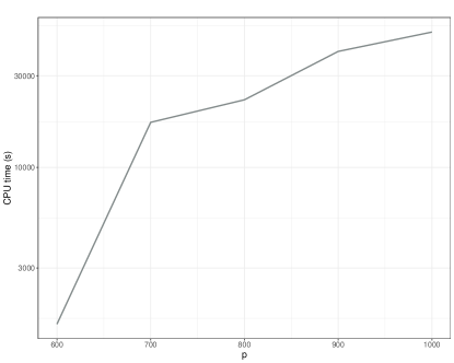
For small , small increases lead to large changes in the AIC score (see Section S.5 of Supplement A). However, for sufficiently large values, the AIC score stabilises as the global shrinkage parameter increases. This can be attributed to the flexibility of the local scale parameters, which compensate for the larger global scale parameter, thus still effectively capturing the magnitude of local effects. Hence, instead of attempting to identify the globally AIC minimising value of , which is computationally expensive, we start with a small value and increase it until the AIC has stabilised. This approach shares similarities with the “dynamic posterior search” of Ročková and George (2018). Formally, using a suitable grid of increasing values , we set to be
for some convergence tolerance .
By selecting the ’s separately, we allow for different sparsity levels across networks. In practice, our jointGHS implementation runs the single-network approach on each network separately (optionally in parallel for computational efficiency), sets using the above procedure, and then uses them in the final joint network run.
5.4 More on the heavy horseshoe tail
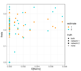
In the joint graphical horseshoe, information is shared through the common latent parameter . In practice, only the full conditional expectation of is used in the ECM algorithm. The larger in (5.2), the larger the CM-updates (10) for the local scales , , and hence the larger the updates for the corresponding precision matrix elements. Thus, a large posterior expected value of signifies strong evidence for the edge being present in all networks. It is also clear from the CM-updates (10) that a conditional expectation of close to zero does not imply that the updates for all the local scales will be close to zero. That is, thanks to the heavy tail of the half-Cauchy distribution, if there is enough evidence from the data, an edge can be identified in an individual network even though the common latent parameter suggests no edge. This is illustrated by Figure 1, which shows the precision elements estimated by the joint graphical horseshoe for networks, plotted against the posterior expectations of the corresponding shared latent parameters . The true networks have edges each, of which in common. Figure 1 shows that the expectation of is only far from zero when an edge is present in both networks. When this expectation is close to zero, i.e., shared information is not found, posterior output still captures edges (i.e. non-zero ) specific to each network. This illustrates how the joint graphical horseshoe estimator can simultaneously share information between networks and capture their differences.
6 Simulations
To evaluate the performance of our approach, we have performed comprehensive simulation studies in R (R Core Team (2013)). We have generated data as close as possible to our omics application of interest, with non-zero partial correlations between and in magnitude and with the scale-free property (i.e. the degree distribution follows a power-law distribution), a common assumption for omics data (Chen and Sharp (2004)). We assess graph accuracy by the precision, i.e., the fraction of the inferred edges that are actually present in the true graph (also known as positive predictive value or complement of the false discovery rate), and by the recall, i.e., the fraction of edges in the true graph that are present in the inferred one (also known as sensitivity or true positive rate). Because the networks inferred by the different methods may result in different sparsity estimates, some consideration is needed when comparing their precision and recall. For example, the recall tends to increase as the number of edges increases, favouring methods that over-select edges. In omics applications, one rather wishes to identify few but highly reliable associations than a large number of associations, many of which will be spurious. In the discussion of the results, we therefore put more emphasis on the precision, and consider the recall to be an informative additional measure, particularly in situations when two methods have comparable precision.
Our numerical experiments are divided into three parts. In Section 6.1, we assess the statistical and computational performance of fastGHS in a single-network setting, comparing it to the Gibbs sampling version of Li et al. (2019a) and to the graphical lasso (Friedman et al. (2008)). In Section 6.2, we demonstrate that, thanks to joint modelling, the accuracy of the jointGHS increases with the number of related networks. Finally, in Section 6.3, we compare the performance of jointGHS to the Bayesian spike-and-slab joint graphical lasso (Li et al. (2019b)), the joint graphical lasso (Danaher et al. (2014)) and GemBag (Yang et al. (2021)). Details on all simulation studies are given in Section S.3 of Supplement A, and the corresponding code is available on Github (https://github.com/Camiling/jointGHS_simulations).
6.1 Comparison of fastGHS with the Gibbs sampling scheme for single networks
In this section we compare the performance of our ECM implementation of the graphical horseshoe to that of the Gibbs sampler by Li et al. (2019a). As a baseline reference, we also provide the results of the widely used graphical lasso algorithm (Friedman et al. (2008)). We consider settings with different numbers of nodes, , and observations, . For each setting, we construct a precision matrix and sample data sets with observations from the corresponding multivariate Gaussian distribution.
6.1.1 Runtime profiling
All above graphical settings give rise to high-dimensional problems: for instance, with and , there are potential edges. For the Gibbs sampling implementation of the graphical horseshoe, a larger , such as , leads to computational problems as the algorithm entails singular updates, likely a result overflow not being properly dealt with (this holds for both the original MATLAB implementation and our translation into R, where the algorithm halts as it attempts to solve a singular system); running examples for this can be found at https://github.com/Camiling/jointGHS_simulations. In this comparison we therefore only consider up to nodes. We emphasise that the limitation for the Gibbs sampler applies to our particular simulation settings. In their simulations, Li et al. (2019a) apply the Gibbs sampler to networks with as many as nodes, but these networks are sparser than ours and have larger partial correlations of magnitude (ours are of magnitude ). This makes the networks strongly identifiable from data, and thus fewer singularity and convergence issues are encountered.
6.1.2 Edge-selection performance
Table 1 indicates the edge-selection performance of fastGHS is comparable to the Gibbs sampler. The two graphical horseshoe implementations perform better than the graphical lasso in terms of both precision and recall in all but one case. For this exception, the graphical lasso has the best performance in terms of precision, likely because it has the sparsest estimate and therefore its inferred edges are more accurate, yet at the expense of a lower recall. The horseshoe-based methods have the best overall performance for a wider range of scenarios.
| Case | True sparsity | p | n | Method | Estimated Sparsity | Precision | Recall |
|---|---|---|---|---|---|---|---|
| 1 | 0.04 | 50 | 100 | Glasso | 0.019 (0.006) | 0.80 (0.12) | 0.37 (0.08) |
| GHS | 0.017 (0.002) |
0.91 |
0.38 (0.05) | ||||
| fastGHS | 0.017 (0.002) |
0.94 |
0.39 (0.05) | ||||
| 2 | 0.04 | 50 | 200 | Glasso | 0.020 (0.003) | 0.88 (0.08) | 0.44 (0.03) |
| GHS | 0.017 (0.002) |
0.98 |
0.42 (0.04) | ||||
| fastGHS | 0.017 (0.002) |
0.99 |
0.43 (0.04) | ||||
| 3 | 0.02 | 100 | 100 | Glasso | 0.011 (0.002) |
0.61 |
0.33 (0.04) |
| GHS | 0.015 (0.001) | 0.49 (0.06) | 0.37 (0.04) | ||||
| fastGHS | 0.015 (0.001) | 0.46 (0.05) | 0.35 (0.03) | ||||
| 4 | 0.02 | 100 | 200 | Glasso | 0.008 (0.001) | 0.86 (0.06) | 0.36 (0.02) |
| GHS | 0.009 (0.001) |
0.91 |
0.40 (0.03) | ||||
| fastGHS | 0.009 (0.001) |
0.93 |
0.41 (0.04) |
As anticipated, our runtime profiling for the Gibbs sampler and our ECM implementation of the graphical horseshoe indicate striking differences. Comparing the two types of inference is not straightforward as they rely on different stopping rules and convergence diagnostics. To alleviate the risk of unfair comparison, we run the Gibbs sampler for a relatively small number of MCMC samples, namely , after burn-in iterations, while for the ECM algorithm, we use a maximum of iterations. Figure 2 shows on a logarithmic scale the CPU time used to infer a network for different numbers of nodes , with observations. For nodes, fastGHS is times faster than the Gibbs sampler. For larger , only the ECM estimator can be used, which in practice is limited only by the available memory to store the matrix updates for , and .
6.2 Increased accuracy with joint modelling
Now that we have established that the performance of our ECM implementation of the graphical horseshoe is comparable to that of the Gibbs sampler, we aim to investigate the gain in statistical power when applying our joint graphical horseshoe estimator, as a function of the number of networks modelled jointly. We use jointGHS to reconstruct graphs with nodes, also applying our single-network method fastGHS on each network separately to serve as baseline. While we simulate scenarios with different degrees of shared information across the graphs (edge disagreement), for a given scenario, the edge disagreement is the same for any pair of networks. Of note, neither the spike-and-slab joint graphical lasso (Li et al. (2019b)) nor the joint graphical lasso (Danaher et al. (2014)) can run within reasonable time for the setting with networks ( hours, see Section S.7.3 of Supplement A). The results are averaged over replicates, and show the precision and recall for the first estimated graph in each setting, reconstructed from observations. All graphs have true sparsity .
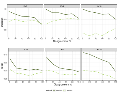
Figure 3 shows the precision and recall for jointGHS and fastGHS as a function of the available information (total number of graphs ) and level of disagreement between them. Although the simulated graph structure remains the same in all settings, the sparsity of the inferred jointGHS graphs varies with total number of graphs and their level of similarity. Hence, to ensure a fair comparison, we obtained single-network estimates with the same sparsity as the joint estimates in each setting, making the fastGHS results vary with both and the level of similarity; we refer to Section S.3 of Supplement A for details.
As expected, the joint approach clearly outperforms the single network approach in terms of both precision and recall, and the improvement increases with the number of graphs , since more shared information is available. This applies to all levels of edge disagreement, including when the graphs have no common edges. This may be explained by the sparsity of the graphs: while the networks do not share any edge, they do share the fact that no edge is present for a large number of pairs . Thus, information is still be shared through conditional expectations of the common ’s being equal to zero. The larger is, the stronger this information is, leading to a large improvement compared to a single network approach.
6.3 Comparison of jointGHS with other joint network inference methods
Now that we have demonstrated the benefit of joint modelling, we next assess the computational and statistical performance of our joint graphical horseshoe estimator, jointGHS, through comparisons with the Bayesian spike-and-slab joint graphical lasso (SSJGL; Li et al. (2019b)), the joint graphical lasso (JGL; Danaher et al. (2014)) and GemBag (Yang et al. (2021)).
6.3.1 Runtime profiling
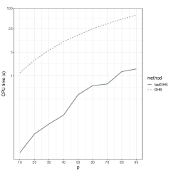
Figure 4 compares the runtime of all methods for a grid of node numbers , networks each with : jointGHS is the fastest of the four methods, for all settings, followed by GemBag, JGL and finally SSJGL. The last two approaches become computationally prohibitive as the number of networks increases. Indeed, Danaher et al. (2014) highlight that the JGL algorithm scales well in problems with only two classes (), as a closed-form solution to the generalised fused lasso problem can be obtained in that case (this also holds for SSJGL). Both SSJGL and JGL use the same alternating direction method of multipliers (ADMM) algorithm to update the precision matrix estimates.
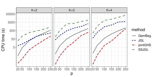
Notably, in their respective simulation studies, Li et al. (2019b) and Danaher et al. (2014) apply their methods to as many as and nodes. However, in the SSJGL numerical experiments, precision matrix elements are sampled from the G-Wishart distribution with degrees of freedom, giving very strong partial correlations ( in absolute value). Similarly, following the precision matrix construction described in the JGL experiments gives partial correlations of in absolute value. This renders the networks strongly identifiable from data, leading to faster convergence than in our simulations where partial correlations and between and . Thus, motivated by realistic biological network strengths, we are considering a more challenging inference problem.
The lower runtime of jointGHS and GemBag can be explained by their EM/ECM implementations, although their higher scalability compared to SSJGL – which also implements an EM algorithm – could be due to their computationally efficient C++ subroutines. Because of these computational limitations, we use relatively small numbers of nodes to make so all methods can run within reasonable time ( hours). Note however that jointGHS successfully completes within this timeframe on examples with nodes (see Section S.7.3 of Supplement A).
6.3.2 Edge-selection performance
We next compare the edge-selection performance of all four methods on problems with graphs of nodes each, and and observations, respectively. We consider six settings, with different levels of graph similarity, i.e., proportion of edges present in both graphs. Namely, we simulate data with similarity varying between edge disagreement (i.e., the same edge set) to edge disagreement (i.e., no common edges). For each setting, we construct two precision matrices with the desired level of similarity and we sample data sets from each of the two corresponding multivariate Gaussian distributions. In all settings, both graphs have true sparsity , corresponding to edges. We report the precision and recall of the final estimate of each method. A threshold-free comparison based on precision-recall curves and corresponding areas under the curves is given in Section S.7.2 of Supplement A.
Table 2 shows the performance of the joint network approaches. The joint graphical lasso JGL, applied with its default AIC-based selection criteria for sparsity- and similarity-selection, has low precision in all settings. The method tends to severely over-select edges, reporting nearly ten times more edges as the number simulated edges: this leads to high recall values but very low precision.
For GemBag, over-selection of edges is not as severe as for (JGL), but the method still reports more edges than the joint graphical horseshoe (jointGHS) and the spike-and-slab joint graphical lasso (SSJGL) in all settings, which results in a lower precision but a higher recall than the two methods. Interestingly, while the first network with seems to benefit from GemBag’s joint modelling, it is not the case of the second network with the largest sample size , as its estimation does not improve as the level of similarity between the two networks increases. Further, due to the larger sample size, GemBag selects more edges for the second network in all settings, which yields a higher recall yet a lower precision than for the first network. Remarkably, the disagreement level (percentage of edges present in only one of the two networks) of the estimated GemBag networks remains almost the same in all settings, and hence does not reflect the different simulated similarity between the two graphs: the method does not appear to adapt to varying network similarity levels, with possibly too much information shared between unrelated networks, yet too little information shared between highly related ones.
The precision of jointGHS is either higher or comparable to that of SSJGL in all settings. In general, jointGHS is more conservative than the other methods, and hence is most suitable for detecting edges with high confidence. This is further exemplified in our extended simulations, particularly in our threshold-free comparisons for sparse edge selection where jointGHS in all settings considered had the highest precision for a given recall level (Section S.7.1 of Supplement A). The graphs estimated by SSJGL are denser, which tends to result in a large recall values: this holds for very similar networks, where SSJGL has the highest recall, yet as network dissimilarity increases, the recall of SSJGL decreases and becomes similar to that of jointGHS. This happens because SSJGL shrinks all precision matrices towards a common structure, thereby over-selecting edges that are absent in some networks while being present in others, as exemplified further in Section 6.3.3. Table 2 indicates that the two networks are estimated by jointGHS as being increasingly different from each other as the simulated level of disagreement increases, while they are invariably estimated as almost identical by SSJGL, even when the true networks are completely unrelated. Of note, the precision of SSJGL deteriorates in settings where the simulated networks share little information, while jointGHS effectively adapts to this setting, maintaining relatively high values of both the precision and recall for completely unrelated networks. As further demonstrated in Section 6.3.3 hereafter, this clear advantage can be attributed to the local scales of the graphical horseshoe, which flexibly capture isolated effects thanks to their heavy Cauchy tails.
| Disagr. | Method | Sparsity | Precision | Recall | Sparsity | Precision | Recall | |||
|---|---|---|---|---|---|---|---|---|---|---|
| 0 | JGL | 63 | 0.312 (0.011) | 0.11 (0.01) | 0.83 (0.05) | 0.269 (0.011) | 0.13 (0.01) | 0.91 (0.04) | ||
| GemBag | 41 | 0.039 (0.006) | 0.65 (0.07) | 0.62 (0.06) | 0.064 (0.008) | 0.49 (0.05) | 0.77 (0.06) | |||
| SSJGL | 0 | 0.025 (0.003) |
0.85 |
0.53 (0.06) | 0.025 (0.003) | 0.85 (0.09) | 0.53 (0.06) | |||
| jointGHS | 17 | 0.017 (0.002) |
0.82 |
0.34 (0.04) | 0.016 (0.001) |
0.93 |
0.38 (0.03) | |||
| 20 | JGL | 65 | 0.310 (0.02) | 0.11 (0.01) | 0.83 (0.05) | 0.266 (0.017) | 0.14 (0.01) | 0.90 (0.04) | ||
| GemBag | 42 | 0.041 (0.007) | 0.61 (0.07) | 0.61 (0.06) | 0.064 (0.01) | 0.47 (0.06) | 0.73 (0.06) | |||
| SSJGL | 1 | 0.025 (0.003) | 0.77 (0.10) | 0.48 (0.05) | 0.025 (0.003) | 0.79 (0.10) | 0.49 (0.05) | |||
| jointGHS | 25 | 0.016 (0.002) |
0.79 |
0.32 (0.04) | 0.016 (0.001) |
0.93 |
0.38 (0.03) | |||
| 40 | JGL | 67 | 0.291 (0.048) | 0.12 (0.02) | 0.82 (0.06) | 0.252 (0.059) | 0.14 (0.05) | 0.83 (0.08) | ||
| GemBag | 49 | 0.038 (0.005) | 0.57 (0.08) | 0.54 (0.05) | 0.066 (0.007) | 0.41 (0.04) | 0.66 (0.05) | |||
| SSJGL | 1 | 0.020 (0.002) |
0.76 |
0.38 (0.04) | 0.020 (0.002) | 0.77 (0.09) | 0.39 (0.05) | |||
| jointGHS | 34 | 0.016 (0.002) |
0.76 |
0.30 (0.04) | 0.010 (0.002) |
0.98 |
0.25 (0.05) | |||
| 60 | JGL | 69 | 0.291 (0.049) | 0.12 (0.02) | 0.82 (0.07) | 0.247 (0.058) | 0.15 (0.05) | 0.84 (0.07) | ||
| GemBag | 48 | 0.039 (0.004) | 0.52 (0.07) | 0.50 (0.05) | 0.064 (0.009) | 0.43 (0.04) | 0.67 (0.06) | |||
| SSJGL | 2 | 0.021 (0.003) | 0.63 (0.09) | 0.33 (0.05) | 0.021 (0.003) | 0.70 (0.08) | 0.37 (0.05) | |||
| jointGHS | 47 | 0.016 (0.002) |
0.74 |
0.29 (0.04) | 0.010 (0.002) |
0.98 |
0.25 (0.05) | |||
| 80 | JGL | 71 | 0.299 (0.040) | 0.11 (0.02) | 0.81 (0.06) | 0.259 (0.046) | 0.14 (0.04) | 0.89 (0.06) | ||
| GemBag | 47 | 0.040 (0.005) | 0.46 (0.07) | 0.46 (0.06) | 0.068 (0.008) | 0.42 (0.05) | 0.70 (0.06) | |||
| SSJGL | 2 | 0.022 (0.004) | 0.52 (0.08) | 0.27 (0.04) | 0.021 (0.003) | 0.60 (0.09) | 0.32 (0.05) | |||
| jointGHS | 59 | 0.015 (0.002) |
0.70 |
0.26 (0.04) | 0.010 (0.002) |
0.98 |
0.25 (0.05) | |||
| 100 | JGL | 72 | 0.313 (0.012) | 0.11 (0.01) | 0.83 (0.05) | 0.251 (0.009) | 0.16 (0.01) | 0.98 (0.02) | ||
| GemBag | 43 | 0.050 (0.004) | 0.34 (0.05) | 0.43 (0.06) | 0.074 (0.006) | 0.48 (0.04) | 0.89 (0.04) | |||
| SSJGL | 3 | 0.029 (0.003) | 0.29 (0.06) | 0.21 (0.03) | 0.029 (0.003) | 0.55 (0.06) | 0.40 (0.05) | |||
| jointGHS | 78 | 0.015 (0.002) |
0.65 |
0.24 (0.04) | 0.013 (0.002) |
0.95 |
0.31 (0.05) | |||
6.3.3 Ability to capture edges on the individual-graph level
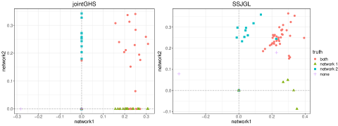
We next provide a more detailed illustration of the benefits of the horseshoe heavy-tailed local scales for capturing graph-specific edges by comparing precision matrix estimates obtained with our joint graphical horseshoe, jointGHS, and the spike-and-slab joint graphical lasso, SSJGL. We use the same data generation procedure as in Section 5.4, with networks reconstructed from two data sets corresponding to graphs with edge agreement, nodes, and and observations, respectively. Both graphs have a true sparsity of .
Figure 5 indicates that jointGHS effectively identifies both common and graph-specific edges. Thanks to its network-specific local scales, when an edge is present in only one of the graphs, the corresponding precision matrix element in the other graph is correctly estimated as null, hence no false positive is reported due to excess shrinkage towards a common graph. As a result, jointGHS is more inclined to false negatives than false positives; in a few instance, it reports edges in only one of the two networks, while they actually present in both. SSJGL displays the opposite behaviour: it shrinks excessively towards a common graph and therefore largely fails to identify the network-specific edges. While the SSJGL does well in capturing edges common to both graphs, an edge in one graph tends to be reported as present in both, resulting in a large number of false positives. This explains its excellent performance for very similar networks, but poorer performance as the similarity between two networks decreases, as discussed in Table 2. Regardless of how similar the networks may be, jointGHS effectively borrows shared information across them, while successfully avoiding over-shrinkage towards a common structure to preserve graph-specific information.
While our simulations have illustrated the flexibility of the joint graphical horseshoe, performing joint modelling of data sets consisting of many highly similar networks and a few unrelated or a priori more loosely similar networks would make little sense. While, thanks to the horseshoe local scales, the risk of the many similar networks dominating the analysis is lower with jointGHS compared to other joint graphical methods – including the spike-and-slab joint graphical lasso (Li et al. (2019b)) and the joint graphical lasso (Danaher et al. (2014)) – it may be helpful to investigators to rule out this scenario. To this end, we outline a Bayesian bootstrapping procedure (Rubin (1981)) in Section S.6 of Supplement A to check whether the joint network estimates are in strong contradiction with each of the single network estimates; this optional routine is implemented in our R package jointGHS.
7 Application to a study of hotspot activity with stimulated monocyte expression
Returning to the monocyte data set from Section 3, we now apply our proposed methodology to estimate conditional independence among the gene levels under genetic control. Specifically, the finding of Ruffieux et al. (2020) about the top hotspot genetic variant (rs6581889, on chromosome ) being persistent across all four monocytic conditions (unstimulated cells, -, LPS 2h- & LPS 24h-stimulated cells) makes a joint graphical approach particularly relevant to study the interplay within and across the different gene networks. The number of genes associated with the top hotspot in each condition was , , and respectively (permutation-based FDR ); hereafter we focus on the genes associated with the hotspot in at least one condition. Further information on the data and preprocessing steps is available in Ruffieux et al. (2020), and details on the analysis presented below can be found in Section S.4 of Supplement A.
We first present and interpret the results obtained by applying jointGHS to jointly estimate the precision matrices, and hence network structures, of the genes in the four conditions. We then describe a comparative study with (i) the classical graphical horseshoe applied separately to each network (using our fastGHS ECM implementation, which scales to this problem), and (ii) a competing joint modelling approach. For the latter comparison, we use GemBag (Yang et al. (2021)), as neither the spike-and-slab joint graphical lasso (Li et al. (2019b)) nor the joint graphical lasso (Danaher et al. (2014)) runs within hours on the data; as previously discussed in Section 6.3.1, both algorithms become substantially slower in problems with classes, due to the absence of closed-form solution for .
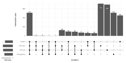
Figure 6 shows the number of edges shared between the different conditions, as inferred by jointGHS. Many edges are common to all four networks, suggesting a high degree of similarity across all monocytic conditions, likely reflecting the effect of the shared hotspot control. Very few edges are shared across three conditions only, but many pairs of conditions have edges that are shared strictly between them. In particular, LPS 2h and LPS 24h have the largest number of shared edges that are not present in the other two conditions, which is expected as they correspond to an exposition to differing durations of a same lipopolysaccharide activation. While LPS is a component of gram-negative bacterial cell walls, is a cytokine important in myobacterial and viral infections (Fairfax et al. (2014)). In addition, and in line with the results of our simulation studies, jointGHS is able to capture many condition-specific edges, with LPS 24h having the highest number of unique edges, possibly because it corresponds to the densest graph across all conditions. These observations call for further biological investigations, which may motivate new mechanistic studies, such as: whether groups of edges shared by two or more conditions pertain to known pathway activation, or whether pathways of genes involved in edges unique to one stimulated condition are indicative of some condition-specific functional mechanisms. We explore such questions in the next sections.
Network-specific activity
A number of the network-specific structures identified by jointGHS warrant close inspection. For example, the Cytochrome C Oxidase Subunit 6A1 (COX6A1) gene has large degree in both LPS 2h and LPS 24h, moderately large degree in , but low degree in the unstimulated condition. The oxidative phosphorylation pathway and immune system processes both include COX6A1 (Wang et al. (2019)), and the gene has been shown to have key functions in the replication of influenza A viruses (Hao et al. (2008)), making it noteworthy that this gene’s activity is found elevated only in the stimulated conditions. Another example pertains to the PHD-finger 1 protein encoding gene (PHF1), which has high degree only in the condition, where it is also found to be controlled by the top hotspot rs6581889. The PHD-finger 1 protein is an essential factor for epigenetic regulation and genome maintenance, and contains two kinds of histone reader modules, a Tudor domain and two PHD fingers (Baker et al. (2008); Liu et al. (2018)). The centrality of PHF1 in the network of the stimulated monocytes suggests a potential role in the immune reaction, and provides a relevant alley for further studies.
Hub genes
Investigating hub genes in the jointGHS networks for the different conditions can help gain better understanding of the immune response driving disease mechanisms. Remarkably, the Autoimmune Regulator (AIRE) gene, which is highly expressed in monocytes, has by far the most links to other genes in all conditions but , where it has the second most (Section S.4 of Supplement A). This gene is known to play an important role in immunity through gene and autoantigen activation and regulation, and negative selection of autoreactive T-cells in the thymus (Liston et al. (2003); Kyewski and Klein (2006); Peterson et al. (2008)). Mutations in this gene have been associated with autoimmune polyendocrinopathy-candidiasis-ectodermal dystrophy (APECED), distinguished by multi-organ autoimmunity (Mathis and Benoist (2007); Akirav et al. (2011)). Similarly, the arylformamidase (AFMID) gene, also known as kynurenine formamidase, is found to have amongst the higher degrees in all four conditions in addition to being associated with the top hotspot in all; it also has a link to LYZ in all four conditions. Arylformamidase is a rate-limiting enzyme in tryptophan conversion, and deficiency is associated with immune system abnormalities (Hugill et al. (2015); Dobrovolsky et al. (2005)). Additional biological results and discussion can be found in Section S.4 of Supplement A.
Hotspot control
We next explore the extent to which the top genetic hotspot rs6581889 influences the conditional independence structure of the genes it controls. Using permutation testing to derive empirical p-values, we find that the subnetwork of genes associated with rs6581889 in each condition has significantly more links than the overall network (), except in the IFN- network, suggesting a hotspot-induced increase in activity. We similarly find that, in all conditions, there is a significant enrichment of genes associated with the top hotspot among the neighbours of the LYZ gene. As LYZ is located a few Kb away from rs6581889, this may suggest a mediation of the hotspot effect on other genes via LYZ – a hypothesis already examined in different studies (Fairfax et al. (2012); Ruffieux et al. (2021)) but which would require experimental validation or dedicated inspection, e.g., with Mendelian randomisation analysis. The findings are summarised in Table 3.
| IFN-gamma | LPS 2h | LPS 24h | Unstim | |||
| Sparsity | Overall | 0.018 | 0.020 | 0.021 | 0.016 | |
| Controlled by top hotpot | 0.019 | 0.042** | 0.183** | 0.022* | ||
| Controlled by top hotspot | Overall | 0.77 | 0.23 | 0.04 | 0.56 | |
| LYZ neighbourhood | 0.78 | 0.42* | 0.33** | 0.77* | ||
| YEATS4 neighbourhood | 0.62 | 0.17 | 0.22** | 0.43 |
Comparison to the single-network analysis
We next aim to assess the possible added value of joint modelling for increasing biological insight by comparing the jointGHS results to those of our single-network ECM implementation of the graphical horseshoe, fastGHS. To obtain comparable networks, we use for fastGHS the same sparsity levels as in the jointGHS estimates, for each condition separately (see Section S.4 of Supplement A for details). The subgraph of hotspot-controlled genes inferred by jointGHS is denser as that inferred by fastGHS in all conditions; a dense graph agrees with the expectation that the hotspot triggers substantial activity among the controlled genes (Ruffieux et al. (2020)). Moreover, both LYZ and YEATS4 have a more central role in the joint network, with more edges to other genes as well as more edges among their neighbours. This lends further support to the mediation hypothesis formulated above. Finally, many genes directly associated with LYZ and YEATS4 have very high degree, suggesting that their interplay with other genes could be relevant for disease-driving mechanisms. All these observations highlight the biological insight gained by sharing information across networks with jointGHS.
Comparison to the GemBag analysis
The comparison of jointGHS with the other joint modelling approach GemBag (Yang et al. (2021)) is also informative. Strikingly, GemBag identifies a strict subset of the edges identified by jointGHS. Moreover, almost all edges are estimated as shared by all four conditions and very few are condition-specific edges; this stands in strong contrast to jointGHS which finds many condition-specific edges. Similarly, the four conditions have an almost complete overlap of top hubs (genes with node degree larger than the percentile) in the GemBag networks, again contrasting the jointGHS networks where the top hubs are mainly network-specific. The biological plausibility of the network specificities discussed above lends support to the argument that jointGHS succeeds at capturing network-specific effects thanks to its horseshoe local scales. Further, LYZ and YEATS4 have very low node degrees in all conditions in the GemBag networks, whereas the two genes are central in the jointGHS networks, with a large number of neighbours, many central neighbours (i.e., hubs) and many top hotspot controlled neighbours, which aligns with evidence from previous studies (Fairfax et al. (2012); Ruffieux et al. (2021)). Further results and details on comparison of GemBag and jointGHS are given in Section S.4 of Supplement A.
While it is reassuring that our method identifies genes known from literature to be relevant, this type of validation is biased towards gene and protein functions that have already been explored. We believe though that jointGHS could serve to generate further unexplored hypotheses about genetic co-regulation and co-expression across the stimulated monocyte networks – this would deserve further follow-up research. More generally, our findings illustrate the potential of the joint graphical horseshoe for gaining deeper insight into the mechanisms at play among large networks of cellular and/or molecular variables for multiple conditions or tissues.
8 Conclusion
We have introduced an efficient ECM algorithm for estimating the precision matrix in the graphical horseshoe, fastGHS, and a novel joint graphical horseshoe estimator for multiple-network inference, jointGHS. Through simulations, we have shown that fastGHS achieves equivalent performance to the fully Bayes graphical horseshoe Gibbs sampler while being substantially more scalable. In the multiple-network setting, we have also shown that jointGHS successfully shares information between networks while capturing their differences, outperforming competing methods such as the joint graphical lasso, GemBag and the spike-and-slab joint graphical lasso, which can be very anti-conservative. This holds for any level of network similarity, even when there is little or no information to share between networks. This clear advantage of the jointGHS can be attributed to the horseshoe heavy-tailed local scales, which are able to adapt even in the absence of shared information, favouring the detection of isolated network-specific edges – to date, no existing joint graphical modelling approach enjoys this property. Hence, jointGHS stands out as a joint approach capable to also pinpoint differences across networks, which, in practice, is often of great interest, sometimes even more than the identification of shared structures. Finally, while our ECM implementation does not provide a fully Bayesian solution, we have demonstrated that this does not affect performance for our primary inference goal, namely edge selection, but now enables estimation for problems of realistic dimensions, which was a key ambition of our work. If desired, parameter uncertainty could still be quantified using an additional bootstrapping procedure.
We have taken advantage of jointGHS to study the gene regulation mechanisms underpinning immune-mediated diseases, using monocyte expression from four immune stimulation conditions. Joint inference on these data identified biologically-supported links, and allowed us to formulate sound mechanistic hypotheses.
There are many possible extensions. For example, given the increasing prevalence of longitudinal studies, a natural continuation would be to propose a time-variant version of the model. Such an extension could be particularly profitable for studies aimed at understanding disease progression, and may also be relevant for the omics application of this paper, where two of the monocyte conditions involved exposure to differing durations of lipopolysaccharide (LPS 2h and LPS 24h). In settings with large numbers of timepoints, autoregression-like approach could be developed, where information would be shared between successive time points.
To conclude, our approach is, to our knowledge, the first to extend graphical models based on global-local priors to the multiple network setting. Additionally, thanks to its remarkable scalability, jointGHS effectively bridges the gap between Bayesian joint network modelling and large-scale inference for real-world studies such as encountered in statistical omics.
Software
The ECM graphical horseshoe approach for single or multiple networks has been implemented in the R packages fastGHS (https://github.com/Camiling/fastGHS) and jointGHS (https://github.com/Camiling/jointGHS), and has all subroutines implemented in C++ for computational efficiency. R code for the simulations and data analyses in this paper is available at https://github.com/Camiling/jointGHS_simulations and https://github.com/Camiling/jointGHS_analysis.
Data
Funding
This research is funded by the UK Medical Research Council programme MRC MC UU 00002/10 (C.L., H.R. and S.R.), Aker Scholarship (C.L.), Lopez–Loreta Foundation (H.R.) and Wellcome Intermediate Clinical Fellowship 01488/Z/16/Z (B.P.F.).
References
- Someren et al. [2002] EP van Someren, Lodewyk FA Wessels, Eric Backer, and Marcel JT Reinders. Genetic network modeling. Pharmacogenomics, 3:507–525, 2002.
- Karczewski and Snyder [2018] Konrad J Karczewski and Michael P Snyder. Integrative omics for health and disease. Nature Reviews Genetics, 19:299–310, 2018.
- Meinshausen and Bühlmann [2006] Nicolai Meinshausen and Peter Bühlmann. High-dimensional graphs and variable selection with the lasso. The Annals of Statistics, 34:1436–1462, 2006.
- Friedman et al. [2008] Jerome Friedman, Trevor Hastie, and Robert Tibshirani. Sparse inverse covariance estimation with the graphical lasso. Biostatistics, 9:432–441, 2008.
- Fan et al. [2009] Jianqing Fan, Yang Feng, and Yichao Wu. Network exploration via the adaptive lasso and scad penalties. The Annals of Applied Statistics, 3:521, 2009.
- Wang et al. [2012] Hao Wang et al. Bayesian graphical lasso models and efficient posterior computation. Bayesian Analysis, 7:867–886, 2012.
- Wang [2015] Hao Wang. Scaling it up: Stochastic search structure learning in graphical models. Bayesian Analysis, 10:351–377, 2015.
- Li et al. [2019a] Yunfan Li, Bruce A Craig, and Anindya Bhadra. The graphical horseshoe estimator for inverse covariance matrices. Journal of Computational and Graphical Statistics, pages 1–24, 2019a.
- Danaher et al. [2014] Patrick Danaher, Pei Wang, and Daniela M Witten. The joint graphical lasso for inverse covariance estimation across multiple classes. Journal of the Royal Statistical Society: Series B (Statistical Methodology), 76:373–397, 2014.
- Guo et al. [2011] Jian Guo, Elizaveta Levina, George Michailidis, and Ji Zhu. Joint estimation of multiple graphical models. Biometrika, 98:1–15, 2011.
- Peterson et al. [2015] Christine Peterson, Francesco C Stingo, and Marina Vannucci. Bayesian inference of multiple gaussian graphical models. Journal of the American Statistical Association, 110:159–174, 2015.
- Li et al. [2019b] Zehang Li, Tyler Mccormick, and Samuel Clark. Bayesian joint spike-and-slab graphical lasso. In International Conference on Machine Learning, pages 3877–3885. PMLR, 2019b.
- Yang et al. [2021] Xinming Yang, Lingrui Gan, Naveen N Narisetty, and Feng Liang. Gembag: Group estimation of multiple bayesian graphical models. The Journal of Machine Learning Research, 22:2450–2497, 2021.
- Ni et al. [2022] Yang Ni, Veerabhadran Baladandayuthapani, Marina Vannucci, and Francesco C Stingo. Bayesian graphical models for modern biological applications. Statistical Methods & Applications, 31:197–225, 2022.
- Lauritzen [1996] S. L. Lauritzen. Graphical models, volume 17. Clarendon Press, 1996.
- Carvalho et al. [2010] Carlos M Carvalho, Nicholas G Polson, and James G Scott. The horseshoe estimator for sparse signals. Biometrika, 97:465–480, 2010.
- Biswas and Mantovani [2010] S. K. Biswas and A. Mantovani. Macrophage plasticity and interaction with lymphocyte subsets: cancer as a paradigm. Nature Immunology, 11:889–896, 2010.
- Fairfax et al. [2014] Benjamin P Fairfax, Peter Humburg, Seiko Makino, Vivek Naranbhai, Daniel Wong, Evelyn Lau, Luke Jostins, Katharine Plant, Robert Andrews, Chris McGee, et al. Innate immune activity conditions the effect of regulatory variants upon monocyte gene expression. Science, 343:1246949, 2014.
- Lee et al. [2014] Mark N Lee, Chun Ye, Alexandra-Chloé Villani, Towfique Raj, Weibo Li, Thomas M Eisenhaure, Selina H Imboywa, Portia I Chipendo, F Ann Ran, Kamil Slowikowski, et al. Common genetic variants modulate pathogen-sensing responses in human dendritic cells. Science, 343:1246980, 2014.
- Kim et al. [2014] Sarah Kim, Jessica Becker, Matthias Bechheim, Vera Kaiser, Mahdad Noursadeghi, Nadine Fricker, Esther Beier, Sven Klaschik, Peter Boor, Timo Hess, et al. Characterizing the genetic basis of innate immune response in tlr4-activated human monocytes. Nature Communications, 5:1–7, 2014.
- Ruffieux et al. [2020] Hélène Ruffieux, Anthony C Davison, Jörg Hager, Jamie Inshaw, Benjamin P Fairfax, Sylvia Richardson, and Leonardo Bottolo. A global-local approach for detecting hotspots in multiple-response regression. The Annals of Applied Statistics, 14:905–928, 2020.
- Yao et al. [2017] Chen Yao, Roby Joehanes, Andrew D Johnson, Tianxiao Huan, Chunyu Liu, Jane E Freedman, Peter J Munson, David E Hill, Marc Vidal, and Daniel Levy. Dynamic role of trans regulation of gene expression in relation to complex traits. The American Journal of Human Genetics, 100:571–580, 2017.
- Fairfax et al. [2012] Benjamin P Fairfax, Seiko Makino, Jayachandran Radhakrishnan, Katharine Plant, Stephen Leslie, Alexander Dilthey, Peter Ellis, Cordelia Langford, Fredrik O Vannberg, and Julian C Knight. Genetics of gene expression in primary immune cells identifies cell type–specific master regulators and roles of hla alleles. Nature Genetics, 44:502–510, 2012.
- Ročková and George [2014] Veronika Ročková and Edward I George. Emvs: The em approach to bayesian variable selection. Journal of the American Statistical Association, 109:828–846, 2014.
- Meng and Rubin [1993] Xiao-Li Meng and Donald B Rubin. Maximum likelihood estimation via the ecm algorithm: A general framework. Biometrika, 80:267–278, 1993.
- Dempster et al. [1977] Arthur P Dempster, Nan M Laird, and Donald B Rubin. Maximum likelihood from incomplete data via the em algorithm. Journal of the Royal Statistical Society: Series B (Methodological), 39:1–22, 1977.
- Makalic and Schmidt [2015] Enes Makalic and Daniel F Schmidt. A simple sampler for the horseshoe estimator. IEEE Signal Processing Letters, 23:179–182, 2015.
- Kook et al. [2021] Jeong Hwan Kook, Kelly A Vaughn, Dana M DeMaster, Linda Ewing-Cobbs, and Marina Vannucci. Bvar-connect: A variational bayes approach to multi-subject vector autoregressive models for inference on brain connectivity networks. Neuroinformatics, 19:39–56, 2021.
- Carvalho et al. [2009] Carlos M Carvalho, Nicholas G Polson, and James G Scott. Handling sparsity via the horseshoe. In Artificial intelligence and statistics, pages 73–80. PMLR, 2009.
- Piironen and Vehtari [2017] Juho Piironen and Aki Vehtari. Sparsity information and regularization in the horseshoe and other shrinkage priors. Electronic Journal of Statistics, 11:5018–5051, 2017.
- Scott and Berger [2010] James G Scott and James O Berger. Bayes and empirical-bayes multiplicity adjustment in the variable-selection problem. The Annals of Statistics, pages 2587–2619, 2010.
- Polson and Scott [2010] Nicholas G Polson and James G Scott. Shrink globally, act locally: Sparse bayesian regularization and prediction. Bayesian statistics, 9:105, 2010.
- Bhadra et al. [2019] A. Bhadra, J. Datta, N. G. Polson, and B. Willard. Lasso meets horseshoe. Statistical Science, 34:405–427, 2019.
- van de Wiel et al. [2019] Mark A van de Wiel, Dennis E Te Beest, and Magnus M Münch. Learning from a lot: Empirical bayes for high-dimensional model-based prediction. Scandinavian Journal of Statistics, 46(1):2–25, 2019.
- Van Der Pas et al. [2014] Stéphanie L Van Der Pas, Bas JK Kleijn, and Aad W Van Der Vaart. The horseshoe estimator: Posterior concentration around nearly black vectors. Electronic Journal of Statistics, 8:2585–2618, 2014.
- Bhadra et al. [2017] Anindya Bhadra, Jyotishka Datta, Nicholas G Polson, and Brandon Willard. The horseshoe+ estimator of ultra-sparse signals. Bayesian Analysis, 12:1105–1131, 2017.
- Akaike et al. [1973] Hirotsugu Akaike, Boris Nikolaevich Petrov, and Frigyes Csaki. Information theory and an extension of the maximum likelihood principle. Second International Symposium on Information Theory, pages 267–281, 1973.
- Ročková and George [2018] Veronika Ročková and Edward I George. The spike-and-slab lasso. Journal of the American Statistical Association, 113:431–444, 2018.
- R Core Team [2013] R Core Team. R: A Language and Environment for Statistical Computing. R Foundation for Statistical Computing, Vienna, Austria, 2013. URL http://www.R-project.org/.
- Chen and Sharp [2004] Hao Chen and Burt M Sharp. Content-rich biological network constructed by mining pubmed abstracts. BMC bioinformatics, 5:1–13, 2004.
- Rubin [1981] Donald B Rubin. The bayesian bootstrap. The Annals of Statistics, pages 130–134, 1981.
- Conway et al. [2017] Jake R Conway, Alexander Lex, and Nils Gehlenborg. Upsetr: an r package for the visualization of intersecting sets and their properties. Bioinformatics, 2017.
- Wang et al. [2019] Lamei Wang, Yu Huang, Xiaolong Wang, and Yulin Chen. Label-free lc-ms/ms proteomics analyses reveal proteomic changes accompanying mstn ko in c2c12 cells. BioMed Research International, 2019, 2019.
- Hao et al. [2008] Linhui Hao, Akira Sakurai, Tokiko Watanabe, Ericka Sorensen, Chairul A Nidom, Michael A Newton, Paul Ahlquist, and Yoshihiro Kawaoka. Drosophila rnai screen identifies host genes important for influenza virus replication. Nature, 454:890–893, 2008.
- Baker et al. [2008] Lindsey A Baker, C David Allis, and Gang G Wang. Phd fingers in human diseases: disorders arising from misinterpreting epigenetic marks. Mutation Research/Fundamental and Molecular Mechanisms of Mutagenesis, 647:3–12, 2008.
- Liu et al. [2018] Ruiqiong Liu, Jie Gao, Yang Yang, Rongfang Qiu, Yu Zheng, Wei Huang, Yi Zeng, Yongqiang Hou, Shuang Wang, Shuai Leng, et al. Phd finger protein 1 (phf1) is a novel reader for histone h4r3 symmetric dimethylation and coordinates with prmt5–wdr77/crl4b complex to promote tumorigenesis. Nucleic Acids Research, 46:6608–6626, 2018.
- Liston et al. [2003] Adrian Liston, Sylvie Lesage, Judith Wilson, Leena Peltonen, and Christopher C Goodnow. Aire regulates negative selection of organ-specific t cells. Nature Immunology, 4:350–354, 2003.
- Kyewski and Klein [2006] Bruno Kyewski and Ludger Klein. A central role for central tolerance. Annu. Rev. Immunol., 24:571–606, 2006.
- Peterson et al. [2008] Pärt Peterson, Tõnis Org, and Ana Rebane. Transcriptional regulation by aire: molecular mechanisms of central tolerance. Nature Reviews Immunology, 8:948–957, 2008.
- Mathis and Benoist [2007] Diane Mathis and Christophe Benoist. A decade of aire. Nature Reviews Immunology, 7:645–650, 2007.
- Akirav et al. [2011] Eitan M Akirav, Nancy H Ruddle, and Kevan C Herold. The role of aire in human autoimmune disease. Nature Reviews Endocrinology, 7:25–33, 2011.
- Hugill et al. [2015] Alison J Hugill, Michelle E Stewart, Marianne A Yon, Fay Probert, I Jane Cox, Tertius A Hough, Cheryl L Scudamore, Liz Bentley, Gary Wall, Sara E Wells, et al. Loss of arylformamidase with reduced thymidine kinase expression leads to impaired glucose tolerance. Biology Open, 4:1367–1375, 2015.
- Dobrovolsky et al. [2005] Vasily N Dobrovolsky, John F Bowyer, Michael K Pabarcus, Robert H Heflich, Lee D Williams, Daniel R Doerge, Björn Arvidsson, Jonas Bergquist, and John E Casida. Effect of arylformamidase (kynurenine formamidase) gene inactivation in mice on enzymatic activity, kynurenine pathway metabolites and phenotype. Biochimica et Biophysica Acta (BBA)-General Subjects, 1724:163–172, 2005.
- Ruffieux et al. [2021] Hélène Ruffieux, Benjamin P Fairfax, Isar Nassiri, Elena Vigorito, Chris Wallace, Sylvia Richardson, and Leonardo Bottolo. Epispot: an epigenome-driven approach for detecting and interpreting hotspots in molecular qtl studies. The American Journal of Human Genetics, 108:983–1000, 2021.
- Kolaczyk [2009] Eric D Kolaczyk. Statistical Analysis of Network Data: Methods and Models. Springer Science & Business Media, 2009.
- Liu et al. [2010] Han Liu, Kathryn Roeder, and Larry Wasserman. Stability approach to regularization selection (stars) for high dimensional graphical models. In Advances in Neural Information Processing Systems, pages 1432–1440, 2010.
- Yang et al. [1996] Ri-Yao Yang, DANIEL K Hsu, and FU-TONG LIu. Expression of galectin-3 modulates t-cell growth and apoptosis. Proceedings of the National Academy of Sciences, 93:6737–6742, 1996.
- Dumic et al. [2006] Jerka Dumic, Sanja Dabelic, and Mirna Flögel. Galectin-3: an open-ended story. Biochimica et Biophysica Acta (BBA)-General Subjects, 1760:616–635, 2006.
- Bernardes et al. [2006] Emerson Soares Bernardes, Neide M Silva, Luciana Pereira Ruas, Jose Roberto Mineo, Adriano Motta Loyola, Daniel K Hsu, Fu-Tong Liu, Roger Chammas, and Maria Cristina Roque-Barreira. Toxoplasma gondii infection reveals a novel regulatory role for galectin-3 in the interface of innate and adaptive immunity. The American Journal of Pathology, 168:1910–1920, 2006.
- Li et al. [2008] Yubin Li, Mousa Komai-Koma, Derek S Gilchrist, Daniel K Hsu, Fu-Tong Liu, Tabitha Springall, and Damo Xu. Galectin-3 is a negative regulator of lipopolysaccharide-mediated inflammation. The Journal of Immunology, 181:2781–2789, 2008.
- Fermino et al. [2011] Marise Lopes Fermino, Claudia Danella Polli, Karina Alves Toledo, Fu-Tong Liu, Dan K Hsu, Maria Cristina Roque-Barreira, Gabriela Pereira-da Silva, Emerson Soares Bernardes, and Lise Halbwachs-Mecarelli. Lps-induced galectin-3 oligomerization results in enhancement of neutrophil activation. PloS ONE, 6:e26004, 2011.
- Nishi et al. [2007] Yumiko Nishi, Hideki Sano, Tatsuo Kawashima, Tomoaki Okada, Toshihisa Kuroda, Kyoko Kikkawa, Sayaka Kawashima, Masaaki Tanabe, Tsukane Goto, Yasuo Matsuzawa, et al. Role of galectin-3 in human pulmonary fibrosis. Allergology International, 56:57–65, 2007.
- Radosavljevic et al. [2012] Gordana Radosavljevic, Vladislav Volarevic, Ivan Jovanovic, Marija Milovanovic, Nada Pejnovic, Nebojsa Arsenijevic, Daniel K Hsu, and Miodrag L Lukic. The roles of galectin-3 in autoimmunity and tumor progression. Immunologic Research, 52:100–110, 2012.
- Huang et al. [2021] Zhong-Yin Huang, Ming-Ming Shao, Jian-Chu Zhang, Feng-Shuang Yi, Juan Du, Qiong Zhou, Feng-Yao Wu, Sha Li, Wei Li, Xian-Zhen Huang, et al. Single-cell analysis of diverse immune phenotypes in malignant pleural effusion. Nature Communications, 12:1–12, 2021.
- Amit et al. [2007] Ido Amit, Ami Citri, Tal Shay, Yiling Lu, Menachem Katz, Fan Zhang, Gabi Tarcic, Doris Siwak, John Lahad, Jasmine Jacob-Hirsch, et al. A module of negative feedback regulators defines growth factor signaling. Nature Genetics, 39:503–512, 2007.
- Rodriguez and Williams [2022] Josue E Rodriguez and Donald R Williams. Bayesian bootstrapped correlation coefficients. The Quantitative Methods for Psychology, 18:39–54, 2022. doi:10.20982/tqmp.18.1.p039.
Appendix A Appendix
Appendix B Derivation of the ECM algorithm with fixed
B.1 Deriving the objective function
Assuming is fixed, the objective function for the graphical horseshoe ECM algorithm is as follows:
| (11) | ||||
B.2 Deriving the E-step
Given the updates for the ’s
| (12) |
the objective function becomes
| (13) | ||||
B.3 Deriving the CM-step
The maximisation of the objective function (B.2) with respect to the ’s is easily found by solving
which has a closed-form solution that gives the updates for :
B.4 Deriving full conditional posteriors for multiple networks
The full conditional posteriors of the ’s depends on the ’s of all networks. They are given by
Appendix C Derivation of the ECM algorithm without fixed
C.1 Full model
When including in the updating scheme, we let it follow a half Cauchy distribution , like the local scales.
C.2 Full conditional posterior
When including in the updating scheme, we use the same reparameterisation trick as for the ’s, i.e. we let and , and get inverse Gamma conditional posteriors for them as well. All other conditional posteriors are as in the setting when is fixed.
C.3 Deriving the objective function
The objective function for the graphical horseshoe ECM algorithm is then as follows:
| (14) | ||||
where denotes and const. is a constant not depending on or .
In the E-step of the algorithm, the conditional expectations in (C.3) are computed. After the E-step is computed, the CM-step performs the maximisation with respect to .
C.4 Deriving the E-step
Given the updates for the ’s and
| (15) | ||||
the objective function becomes
| (16) | ||||
C.5 Deriving the CM-step
The maximisation of the objective function (C.4) with respect to is easily found by solving
which has a closed-form solution that gives the update
| (17) |
Similarly, we can maximise (C.3) with respect to the ’s to find the updates for :
which is solved by
The updates for are as in B, but with the fixed replaced by the latest update .
C.6 Deriving full conditional posteriors for multiple networks, with ’s fixed
The full conditional posteriors of the ’s depends on the ’s of all networks. They are given by
C.7 Deriving full conditional posteriors for multiple networks, without ’s fixed
When including the ’s in the updating scheme, we let them follow half Cauchy distributions , like the local scales. Similarly, like for the local scales, we introduce the latent variables for the ’s with a similar parameterisation and , and get inverse Gamma full conditional posteriors for them as well. The global scales are kept network-specific to allow for different sparsity levels across networks.
The full conditional posteriors of the ’s depends on the ’s of all networks. They are given by
In the E-step, the ’s follow the same distribution as in the standard graphical horseshoe within each network. This means that
In the CM-step for multiple networks, the global shrinkage parameter for each graph is updated as the maximising value (17) within the network:
Appendix D Simulation study details
To evaluate the performance our proposed methodology, we have done comprehensive simulation studies in R (R Core Team [2013]). We have used our R packages fastGHS and jointGHS to perform the single-network graphical horseshoe ECM routine and the joint graphical horseshoe ECM routine respectively, and the code for the simulations is available on Github (https://github.com/Camiling/jointGHS_simulations).
D.1 Single network inference
The first part of the simulation studies compares our graphical horseshoe ECM implementation (fastGHS) to the graphical horseshoe Gibbs sampler and the graphical lasso. The performance of the methods is assessed on multivariate Gaussian simulated data sets.
Generating networks and data
We aim to generate data similar to our omic application of interest. We have done this using the R package huge. The package provides the function huge.generator(), which generates multivariate Gaussian data with the scale-free property as it is a known characteristic of multiomic data (Kolaczyk [2009]). Given a number of vertices, huge constructs a precision matrix with edges. For a desired number of observations , a data set can then be generated from the resulting multivariate Gaussian distribution with covariance matrix and expectation vector . This results in a by data matrix , where each column corresponds to a node. As for the values of the non-zero partial correlations, we let them be in , a range we found to reflect the values observed in our omic application. Such data is generated times. In our simulations, we consider different settings, i.e., different combinations of and . When , the final graph has edges and thus a sparsity of . When , the sparsity of the graph is .
Data analysis details
In our simulation study, we wish to compare the graph reconstruction accuracy of the Gibbs sampling implementation of Li et al. [2019b] to our ECM implementation of the graphical horseshoe (fastGHS). We also include the graphical lasso of Friedman et al. [2008], a state-of-the-art frequentist method for Gaussian graph reconstruction. For each setting we consider, and each generated data set, we obtain a precision matrix estimate from the data of interest for each of the methods.
We perform the ordinary graphical lasso using the R function huge, while we perform the Gibbs sampling procedure using the code of Li et al. [2019b] translated by us from MATLAB to R. A translation is necessary for us to perform the simulation study in R, but we have ensured that it gives identical results to those of the original MATLAB implementation.
The sparsity level of the graphical lasso is selected using the Stability Approach to Regularisation Selection (StARS), a selection method based on model stability (Liu et al. [2010]), with variability threshold . For the Gibbs sampling procedure of Li et al. [2019b], we draw MCMC samples after burn-in iterations. In fastGHS, we use a convergence tolerance threshold of for the precision matrix estimate and an AIC convergence threshold of for the global scale parameter selection. The results are averaged over the simulations for all settings, and we report the precision and recall, as well as the sparsity of the estimates.
Computational time simulation details
To illustrate the scalability of our ECM implementation for the graphical horseshoe, we save the CPU time used to infer a network for different numbers of nodes , using Gaussian graphical data sets with observations. We limit ourselves to , to permit comparison to the less scalable Gibbs sampler of Li et al. [2019b]. We run all methods on a 16-core Intel Xeon CPU, 2.60 GHz. We use the same parameters as for the single network simulation study, and consider the time used for one run, i.e. for a given value of in the joint graphical horseshoe or one initial value in the Gibbs sampler.
D.2 Multiple network inference
Generating Gaussian graphs and data of specific similarity
We generate data for the joint graphical horseshoe simulation study using the same method as in 6.1 in the main manuscript, with the huge package in R to generate graphs and drawing data from the corresponding multivariate Gaussian distributions. The main difference is that we now have graphs instead of one. Because we wish to investigate different settings with various similarity of the true graph structures, we can not generate the graph structures independently. Starting by generating the first graph using huge, we instead modify its precision matrix in order to obtain a second graph with the desired level of similarity. Specifically, for the initial precision matrix we create, we permute a certain percentage of the edges by randomly reallocating them. This allows us to generate graphs of various similarity, ranging from edge disagreement (i.e. the same edge set) to edge disagreement (i.e. no common edges). In all settings, both graphs have true sparsity . For each pair of graphs, we sample data sets from each of the two corresponding multivariate Gaussian distributions, with observations for the first graph and observations for the second.
Data analysis details
For each pair of generated data sets, we use the different joint graph reconstruction methods to obtain precision matrix estimates and assess their performance. In addition to our joint graphical horseshoe approach, we consider the Bayesian spike-and-slab joint graphical lasso of Li et al. [2019b] and the joint graphical lasso of Danaher et al. [2014]. Li et al. [2019b] provide R code for the Bayesian spike-and-slab at https://github.com/richardli/SSJGL, and the joint graphical lasso is implemented by Danaher et al. [2014] in the R package JGL. Yang et al. [2021] provide R code for GemBag at https://github.com/xinming104/GemBag.
The spike-and-slab joint graphical lasso (SSJGL) has a wide range of parameters that must be selected, and we use the values Li et al. [2019b] use for their own simulations, including an EM convergence tolerance of . In the joint graphical lasso, the sparsity- and similarity controlling parameters must be selected. We do this using the approach suggested by Danaher et al. [2014], considering a grid of two parameters to find the values minimising their proposed adapted AIC score. For GemBag, we use the BIC to select the hyperparameters and , as suggested by Yang et al. [2021]. For the other hyperparameters, we use the values suggested and used by Yang et al. [2021] in their simulations.
In our joint graphical horseshoe approach, we use a convergence tolerance threshold of for the precision matrix estimate and an AIC convergence threshold of for the global scale parameter selection. For both graphs, the results are averaged over the simulations for all settings and methods, and we report the precision and recall as well as the sparsity of the estimates. When comparing jointGHS and fastGHS, we get the fastGHS estimate of each network to the same sparsity as the corresponding jointGHS estimate by setting the global scale parameter to a small value, and slowly increasing it until the same sparsity is achieved.
Appendix E Monocyte data
E.1 Data analysis details
For the jointGHS application, we use a convergence tolerance of for the precision matrices. We use the same tolerance when applying fastGHS to each condition separately. Due to the large size of the problem, with potential links to be inferred, we use a looser AIC convergence threshold of for the global scale parameter selection to speed up computations. As previously discussed, inference is not very sensitive to this choice: a wide range of global scale parameter values tend to give similar results. When comparing the results from jointGHS and fastGHS, we get the fastGHS estimate of each condition to the same sparsity as the corresponding jointGHS estimate by setting the global scale parameter to a small value, and slowly increasing it until the same sparsity is achieved.
E.2 Additional results
Model parameters
Figure E.1 shows the scaled precision matrix elements of the jointGHS estimates plotted against the common latent parameters in all four conditions. We see that while many edges are found to be in common meaning information has been shared, there are still many network-specific edges that have been inferred. Thanks to the heavy horseshoe tail, we are able to capture these edges even though no common information about them is found between the conditions.
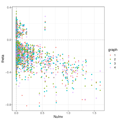
Degree distribution
Table E.1 shows the node degree of the genes with degree larger than the percentile in the respective jointGHS networks of the different conditions. A complete list of all node degrees is given in Supplement B, and can be used for further investigation.
| IFN-gamma | LPS-2h | LPS-24h | Unstimulated | |||||||
|---|---|---|---|---|---|---|---|---|---|---|
| Gene | Degree | Gene | Degree | Gene | Degree | Gene | Degree | |||
| ACBD5* | 33 | AIRE | 37 | AIRE | 38 | AIRE* | 40 | |||
| AIRE* | 25 | B3GNT5 | 28 | TNK2 | 25 | AFMID* | 33 | |||
| AFMID* | 24 | AFMID* | 26 | AFMID* | 25 | PHRF1 | 24 | |||
| LGALS3 | 23 | LGALS3 | 24 | COX6A1 | 24 | LGALS3 | 23 | |||
| SLC3A2 | 20 | COX6A1 | 24 | LGALS3 | 22 | NBPF8 | 20 | |||
| PHF1* | 20 | ACBD5 | 24 | TBC1D9 | 21 | AKR1D1* | 20 | |||
| YEATS4* | 18 | AFTPH | 22 | EPSTI1 | 21 | AFTPH | 20 | |||
| PTPLAD2* | 18 | PRPF8 | 21 | CYP27A1 | 21 | GIMAP1 | 19 | |||
| GIMAP1 | 18 | EPSTI1 | 21 | YEATS4* | 20 | STAG3L3 | 18 | |||
| COPZ1* | 18 | IMPDH1 | 19 | STK24 | 20 | SLC3A2 | 18 | |||
| TNK2 | 17 | GIMAP1 | 19 | STAG3L3 | 20 | ADAMTS4* | 18 | |||
| STK24 | 17 | BIRC3 | 19 | AFTPH | 20 | VHL* | 17 | |||
| SORL1 | 17 | TBC1D15 | 18 | CCL20 | 19 | SGK3* | 17 | |||
| SNX17 | 17 | SORL1 | 18 | TNFSF14 | 18 | GSDM1* | 17 | |||
| RELB | 17 | SLC3A2 | 18 | SORL1 | 18 | ZNF845 | 16 | |||
| CYP27A1 | 17 | CYP27A1 | 18 | SLC3A2 | 18 | YEATS4* | 16 | |||
| NLRP3 | 16 | BFAR | 18 | RELB | 18 | TBC1D9 | 16 | |||
| NBPF8 | 16 | SNX17 | 17 | PTPLAD2 | 18 | KIAA0101* | 16 | |||
| KIAA0101* | 16 | PION | 17 | GNB4 | 18 | JARID2 | 16 | |||
| EPSTI1 | 16 | NOD1 | 17 | CRTC3 | 18 | GLTSCR1 | 16 | |||
| COX6A1 | 16 | NLRP3 | 17 | CD72 | 18 | PTPLAD2 | 15 | |||
| B3GNT5 | 16 | ALPP | 17 | BATF3 | 18 | LYZ* | 15 | |||
| SMC4 | 15 | ZYX | 16 | TLK1 | 17 | FLJ38717 | 15 | |||
| PRPF8* | 15 | SGK3 | 16 | SMC4 | 17 | COX19 | 15 | |||
| MAFF* | 15 | RELB | 16 | IMPDH1 | 17 | ALPP* | 15 | |||
| LOC728457 | 15 | NBPF8 | 16 | HNRPR | 17 | AGTRAP* | 15 | |||
| IMPDH1* | 15 | LOC641522 | 16 | DENND4C | 17 | ACBD5* | 15 | |||
| GSDM1* | 15 | KIAA0101* | 16 | COPZ1 | 17 | TLK1 | 14 | |||
| BATF3 | 15 | HNRPR | 16 | CHRNA5* | 17 | SORL1 | 14 | |||
| TNFSF15* | 14 | GTF2IRD2B | 16 | C4orf34 | 17 | RELB | 14 | |||
| STAG3L3* | 14 | AGTRAP | 16 | TPM4 | 16 | PCDHB9 | 14 | |||
| SGK3* | 14 | SNX17 | 16 | NLRP3 | 14 | |||||
| NFIL3 | 14 | PLEKHB2 | 16 | KLHL8* | 14 | |||||
| HNRPR | 14 | PHRF1 | 16 | IMPDH1 | 14 | |||||
| FLJ38717* | 14 | NFIL3 | 16 | IL12RB1 | 14 | |||||
| BIRC3* | 14 | C4orf34* | 14 | |||||||
| AFTPH* | 14 | C12orf43 | 14 | |||||||
| ADAMTS4* | 14 | BIRC3* | 14 | |||||||
Hub genes
This discussion complements the hub gene subsection found in the main manuscript. A gene with many links consistent across all conditions is Galectin-3 (LGALS3), whose expression is found to modulate T-cell growth and apoptosis (Yang et al. [1996]). Studies indicate that it affects numerous biological processes through specific interactions with a variety of intra- and extracellular proteins, and has a regulatory role in both innate and adaptive immunity (Dumic et al. [2006], Bernardes et al. [2006]). It has been found to be a negative regulator of lipopolysaccharide (LPS) mediated inflammation (Li et al. [2008], Fermino et al. [2011]), and lack of Galectin-3 has been directly linked to higher levels (Nishi et al. [2007], Radosavljevic et al. [2012]). Finally, the Aftiphilin (AFTPH) gene has many links in all conditions, including to YEATS4. Aftiphilin has been found to be differentially expressed in the immune cells of tumor patients, suggesting it might affect tumor development through immune cell regulation (Huang et al. [2021]).
LYZ and YEATS4 and their neighbours
To investigate the role of LYZ and YEATS4 in the different conditions, Figure E.2 shows their edges in the four conditions. It is clear that the two genes have a number of neighbours, and thus are relatively influential in the networks. These neighbours are fairly spread out on the chromosomes, in accordance with our expectations about the hotspot-induced effect of LYZ and YEATS4 on distal genes (Ruffieux et al. [2020]). While several edges are common to all conditions, we see that jointGHS identifies many edges on the specific condition level. Further, we see that a lot of the edges represent negative partial correlations, implying that the two genes could have a role in the down-regulation as well as the up-regulation of the other genes.
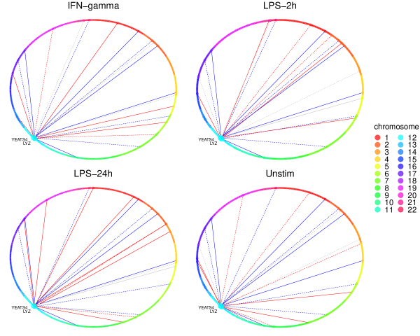
Investigating the neighbourhood of LYZ and YEATS4 in each condition can also be useful for understanding the possible mediation effect of LYZ and YEATS4. Table E.2 shows the node degree of all neighbours in the jointGHS networks of the different conditions. As we see, AFMID is a neighbour of LYZ in all four conditions. Given its central role in each network, this potential interplay between LYZ and AFMID is noteworthy. Another notable observation is that PHF1 is a neighbour of LYZ or YEATS4 only in . Given its importance only in this network, the possible association between LYZ and PHF1 may provide further insight into the role of this gene. Another neighbour of LYZ in all conditions is MAF BZIP Transcription Factor F (MAFF), which is a regulator for growth factor signaling (Amit et al. [2007]). We also observe that AFTPH, which we found to have a high degree in all conditions, is a neighbour of YEATS4 in all four conditions.
| LYZ | ||||||||||
| IFN-gamma | LPS-2h | LPS-24h | Unstimulated | |||||||
| Gene | Degree | Gene | Degree | Gene | Degree | Gene | Degree | |||
| AFMID* | 24 | AFMID* | 26 | AFMID* | 25 | AFMID* | 33 | |||
| LGALS3 | 23 | LGALS3 | 24 | YEATS4* | 20 | PHRF1 | 24 | |||
| PHF1* | 20 | NDUFV3* | 13 | MAFF | 14 | LGALS3 | 23 | |||
| NBPF8* | 16 | MAFF* | 12 | SNRNP48 | 12 | LOC202781 | 13 | |||
| MAFF* | 15 | TPM3 | 11 | MBD4 | 12 | KLHL28* | 11 | |||
| KLHL28* | 11 | SNRNP48 | 11 | LRRFIP1 | 10 | SNRNP48* | 10 | |||
| SNRNP48* | 9 | LOC653086 | 11 | KLHL28* | 10 | NCAPD2* | 10 | |||
| LIN52* | 9 | MBOAT2 | 10 | LOC100128098 | 8 | MAFF* | 8 | |||
| LOC100128098* | 7 | KLHL28* | 10 | KIAA1751 | 8 | LOC100128098* | 7 | |||
| TBCCD1 | 7 | TBCCD1* | 6 | |||||||
| MINK1 | 7 | RAG1AP1* | 6 | |||||||
| LOC100128098* | 6 | MEFV* | 5 | |||||||
| MINK1* | 4 | |||||||||
| YEATS4 | ||||||||||
| IFN-gamma | LPS-2h | LPS-24h | Unstimulated | |||||||
| Gene | Degree | Gene | Degree | Gene | Degree | Gene | Degree | |||
| AIRE* | 25 | AIRE | 37 | LGALS3 | 22 | AFTPH | 20 | |||
| LGALS3 | 23 | AFTPH | 22 | TBC1D9 | 21 | TBC1D9 | 16 | |||
| COPZ1* | 18 | IMPDH1 | 19 | AFTPH | 20 | GLTSCR1 | 16 | |||
| RELB | 17 | SORL1 | 18 | TLK1 | 17 | TLK1 | 14 | |||
| IMPDH1* | 15 | TBC1D9 | 15 | IMPDH1 | 17 | IMPDH1 | 14 | |||
| AFTPH* | 14 | HIST1H2BD | 15 | COPZ1 | 17 | USP49* | 13 | |||
| TLK1 | 13 | TLK1 | 14 | AKR1D1 | 15 | COPZ1 | 13 | |||
| SLC4A5* | 13 | COPZ1 | 13 | SC4MOL | 14 | BFAR | 13 | |||
| TBC1D15 | 12 | ZNF131* | 11 | ZNF131* | 11 | SLC4A5* | 11 | |||
| CHST12* | 12 | MEFV | 10 | LYZ* | 11 | TP53BP2* | 8 | |||
| SMCR5* | 11 | TP53BP2* | 9 | ZNF738 | 10 | DDX51* | 7 | |||
| LYRM7 | 11 | TMEM106A | 9 | LRRFIP1 | 10 | TMEM106A* | 6 | |||
| TP53BP2* | 10 | XRCC2 | 9 | TMEM128* | 5 | |||||
| SC4MOL* | 10 | TP53BP2* | 9 | CDK5RAP2 | 5 | |||||
| TMEM106A* | 9 | TMEM106A | 9 | |||||||
| TBC1D9 | 9 | MFSD11 | 8 | |||||||
| DDX51* | 7 | |||||||||
| TIPRL | 6 | |||||||||
It can be relevant to investigate whether the neighbours of LYZ and YEATS4 tend to be have more associations with the top hotspot. Table 3 in the main manuscript shows the proportion of the neighbours of LYZ and YEATS4 respectively that are mediated by the top hotspot in each condition, and compares it to the total proportion of top hotspot controlled genes. We use permutation testing to assess whether more of the neighbours of each gene are controlled by the top hotspot than we would expect from a gene set of the same size; by randomly sampling gene sets with the same size as the neighbourhood, we calculate empirical p-values for the observed proportion of controlled neighbours. We see that YEATS4 does not have significantly more mediated neighbours than the overall fraction, except in LPS 24h. LYZ, on the other hand, has, at a significance level , more mediated neighbours in all conditions.
Figure E.3 shows the density of the degree distribution of the jointGHS graph of each condition, as well as the degree of LYZ and YEATS4. It appears that the degree distribution of the unstimulated network has more density on lower degrees, which is reasonable considering the unstimulated network is the sparsest among the four. As we see, the two genes have a relatively high degree in all conditions.
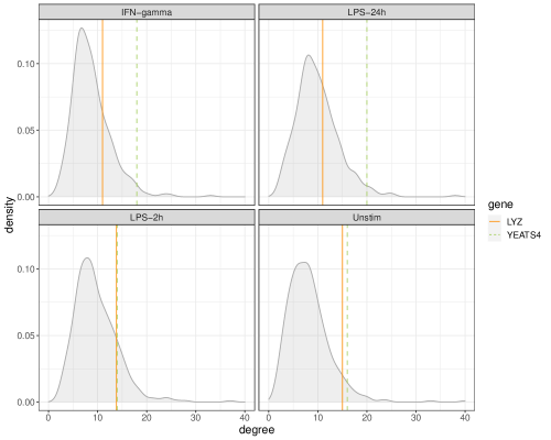
Top-hotspot mediated genes
Investigating whether the genes controlled by the top hotspot have more associations with each other can be insightful. In Table 3 in the main manuscript, we find the sparsity of the subnetwork of genes that are mediated by the top hotspot in each condition, and compares it to the sparsity of the whole network. We use permutation testing to assess whether the subnetwork of top hotspot controlled genes is denser than we would expect from a subnetwork of the same size; by randomly sampling subnetworks with the same size, we calculate empirical p-values for the observed sparsity. We see that the empirical p-value is for all conditions except , implying the subnetworks are indeed denser in these conditions. While the difference is relatively small in the unstimulated network, it is larger in the LPS ones and in particular in LPS 24h.
Comparison to results from single network analysis
Table E.3 shows the sparsity of the estimated jointGHS graphs of the different conditions, as well as the percentage of the inferred edges that the jointGHS and fastGHS estimates at the same sparsity agree on. Figure E.4 shows an upset plot (Conway et al. [2017]), an alternative to a venn diagram that shows the number of edges shared between the inferred networks of each condition, for fastGHS and jointGHS separately. For each intersection, the number of edges shared only by the corresponding conditions is shown. It indicates that many edges are common to all four networks, meaning that the joint method has identified a fair amount of shared information. Compared to the fastGHS networks, we see that the intersection of edges present in all four conditions is larger in the jointGHS networks. This is as expected, as we, with the joint method, are better equipped to identify what is common and borrow information.
| IFN-gamma | LPS-2h | LPS-24h | Unstimulated | |
|---|---|---|---|---|
| Sparsity | 0.018 | 0.020 | 0.021 | 0.016 |
| Edge agreement with fastGHS | 66.8 | 64.6 | 65.9 | 62.3 |
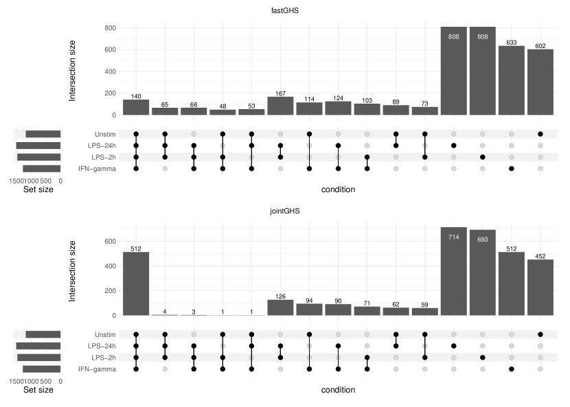
To understand more about what differs between the single and the joint estimates, we have a closer look at the genes controlled by the top hotspot rs6581889. The left panel of Figure E.5 compares the fastGHS and jointGHS density of the degree distribution of the subnetwork of genes controlled by the top hotspot in each condition. The density plots with the mean and median lines suggest that the jointGHS distribution is more shifted to the right in all conditions, implying that amongst the genes controlled by the top hotspot, the joint method identifies an overall higher activity level in terms of associations to other genes. This agrees with what we would expect, with the hotspot triggering substantial gene activity (Ruffieux et al. [2020]).
We next investigate the role of LYZ and YEATS4 in the networks inferred by the two methods. In particular, we want to investigate if their role is common to all four conditions. To this end, we compare the neighbourhood status (with respect to the two genes) of the edges common to all conditions, namely, how close an edge is to one of the two genes. If an edge is between LYZ or YEATS4 and another gene, that edge has order . If an edge is between two other genes where at least one of them is a neighbour of LYZ or YEATS4, that edge has order , and so on. Only the edges found to be common in all conditions in jointGHS but not in fastGHS are shown, and vice versa. The results from the comparison are shown in the right panel of Figure E.5. The edges identified by jointGHS but not fastGHS are in much closer proximity to LYZ or YEATS4, implying that the joint method identifies a stronger effect from the two genes, which agrees with previous findings (Ruffieux et al. [2020]). Similarly, there is not a single edge between LYZ or YEATS4 and other genes identified by fastGHS but not jointGHS, while the opposite is not true. This again implies that the joint method is able to identify more of the hotspot-mediated relationships.
We have now investigated what differs between the networks informed by fastGHS and jointGHS, but what about the edges the two methods agree on? The alluvial diagram in figure E.6 compares the order to the edges common to all conditions, and that fastGHS and jointGHS agree on, using the same definition of order as above. It shows that the two methods agree completely on all first order edges, meaning the direct effect of LYZ and YEATS4 on the other genes in this case has sufficient evidence in the data to be captured even with the single-network approach. We also observe that the edges tend to have a lower order in the jointGHS estimates, implying a stronger influence from LYZ and YEATS4 has been captured. This strong effect of the two genes observed in the jointGHS estimates agrees more with previous findings in this data set (Ruffieux et al. [2020]). In general, we see that two methods disagree more on the higher-order edges, where the effect of the LYZ and YEATS4 can be said to be weaker. In such a setting, a joint approach that gains statistical power by sharing information between conditions can be highly useful, helping us gain more insight not only into the effects of LYZ and YEATS4 on other genes but also role of the affected genes. In particular, many genes directly associated with LYZ and/or YEATS4 have a very high degree, highlighting their interplay with other genes as potentially relevant for the disease-driving mechanisms.
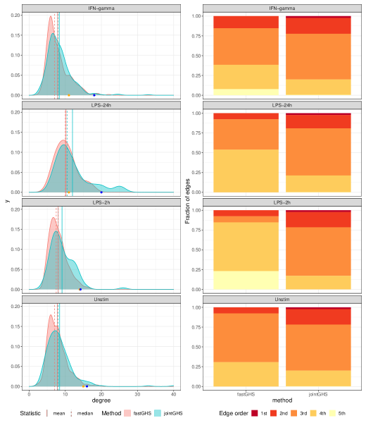
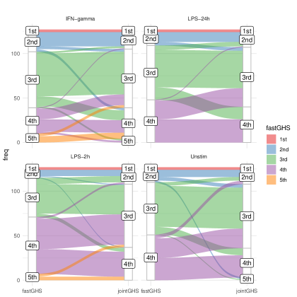
E.3 Application of GemBag
E.3.1 Data analysis details
E.3.2 Resulting networks
The resulting GemBag networks all have sparsity , which notably is much sparser than the jointGHS networks. Figure E.7 shows the number of edges solely shared between the inferred GemBag networks of each condition. As we see, mainly common edges for all four conditions are identified, and very few condition-specific edges. This stands in strong contrast to the jointGHS estimates, where a large number of condition-specific edges were found.
Comparing the GemBag networks to those found by jointGHS, we find that all of the edges that were identified by GemBag were also identified by jointGHS, making the edges identified by GemBag a subset of the edges identified by jointGHS.
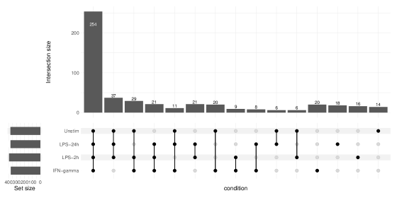
E.3.3 Hub genes
Table E.4 shows the number of genes with node degree larger than the percentile (hubs) in the respective networks of the different conditions, for the jointGHS and the GemBag networks. The number of hubs common to all four conditions is shown as well, for both methods. As we see, while the number of hubs in each condition is comparable for the two methods, there is a far bigger overlap in top hubs in the GemBag networks (24 common hubs) than the jointGHS networks (8 common hubs). This again illustrates how GemBag identifies less condition specific interactions and traits than jointGHS.
| IFN-gamma | LPS-2h | LPS-24h | Unstimulated | All conditions | |
|---|---|---|---|---|---|
| jointGHS | 38 | 31 | 35 | 34 | 8 |
| GemBag | 34 | 36 | 34 | 29 | 24 |
E.3.4 Hotspot control
Figure E.8 shows the density of the degree distribution of the GemBag graph of each condition, as well as the degree of LYZ and YEATS4. As we see, the two genes have a very low node degree in all four conditions, unlike in the jointGHS networks where they are central (Figure E.3). While the GemBag networks are sparser, and thus fewer edges can be expected, LYZ and YEATS4 still have a very low node degree relative to the overall degree distribution.
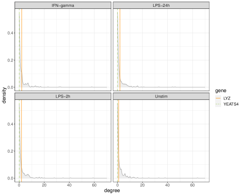
In fact, YEATS4 has node degree in all four conditions. Thus, the GemBag networks give no evidence for the mediation of the hotspot effect on other genes via this gene. Similarly, GemBag gives no evidence for an effect via LYZ. While these two genes were central in the jointGHS networks, with a large number of neighbours, many central neighbours (i.e. hubs) and many top hotspot controlled neighbours, the GemBag networks do not capture this hotspot mediated effect which had been reported by Fairfax et al. [2012] and Ruffieux et al. [2021].
Appendix F More on the choice of global shrinkage parameter
This section supplements Sections 2 and 4 in the main manuscript.
F.1 The deflation issue of the global shrinkage
Figure F.9 illustrates how the global shrinkage parameter shrinks to zero after just a few iterations, regardless of its initial value, when it is updated in the ECM algorithm. The Gaussian graphical data is generated using the procedure described in Section D, with nodes and observations in each data set.
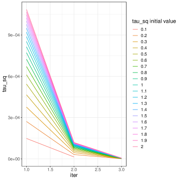
F.2 The issue of under-selection
Our ECM approach does not tend to over-select edges. Figure F.10 shows two trace plots for a Gaussian graphical data set with nodes and observations, one considering only small values of and the other larger. Since we ultimately are interested in the partial correlations, we disregard the scale and look at the size of the scaled precision matrix elements . By comparing how these elements change as increases, the plot illustrates that over-selection of edges is not a concern. This can in part be explained by the fact that the local scale parameters adapt to the global shrinkage parameter, making the model flexible with respect to the choice of as long as it is large enough to avoid overshrinkage to zero. Indeed, for small values of we see that very few edges are captured, and the estimates deviate more from their true value of . It is clear that we should take care to ensure the global scale parameter is not too small. If high computational efficiency is desired, fixing it to a large value is possible. However, for general use we propose a data-driven way to select the parameter.
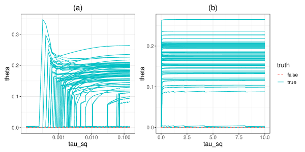
F.3 Avoiding under-selection with the AIC
Figure F.11 shows plots of the sparsity, precision and recall of ECM graphical horseshoe network estimates for different values of the fixed global shrinkage parameter , and for two data sets with (a) and with true graph sparsity and (b) and with true graph sparsity . The estimated sparsity grows with , but only to a certain point. For large enough values of the global shrinkage parameter, the results are the same in terms of precision and recall. On the other hand, too small values of can lead to severe under-selection of edges and very variable results.
Figure F.12 shows the second setting (b) for , where the values corresponding to the found by our AIC selection approach are marked as points. This rule leads to satisfactory results in terms of both precision and recall. A smaller value of would result in reduced accuracy, and a larger value would not improve the estimate further.
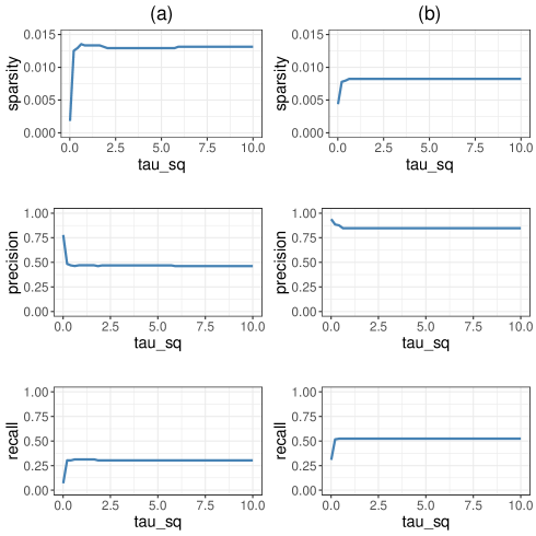
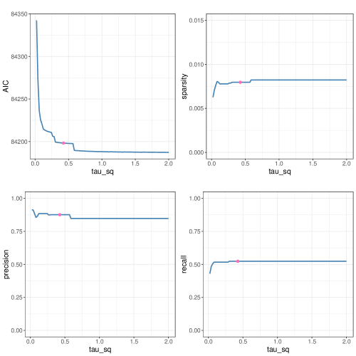
Appendix G Posterior checks with the Bayesian bootstrap
While the joint graphical horseshoe adapts well to the level of similarity between networks, issues may arise when the joint analysis is performed on a set with many highly similar networks and a few unrelated or less similar networks. In such a case, the highly similar networks might dominate the analysis through the common latent variables . We have seen that, due to the heavy tail of the horseshoe, a small does not detoriate inference since the local scales still can escape and identify edges individually on the network level. However, a large tends to lead to non-zero precision matrix elements for all networks. A setting with many highly similar and a few unrelated or less similar network can result in large for the edges common to the highly similar networks, risking wrongly included edges and thus reduced accuracy for the less similar ones.
To account for this possibility, after performing a joint network analysis it should be possible to check whether the edges of the joint network estimates strongly contradict the single network estimates. This could indicate that a joint approach is not suitable.
For this purpose, we propose an approach for performing a posterior check for the suitability of a joint analysis. This check is implemented in our R package jointGHS. This extra step is more computationally demanding, but is optional and only necessary if there is doubt about the suitability of a joint approach.
G.1 Bayesian bootstrap procedure
We propose to use Bayesian bootstrapping (Rubin [1981]) to assess the suitability of a joint analysis. Specifically, for each network and each inferred edge found in the joint analysis, we assess whether the corresponding precision matrix element from the joint analysis is plausibly non-zero given its posterior Bayesian bootstrap distribution in the single network version.
In order to obtain a bootstrap sample for , we start by drawing weights from the Dirichlet distribution with categories and parameters , i.e., the flat Dirichlet distribution. The resulting weight vector is used to weigh the observations in the by observation matrix . For notational simplicity, we will from now refer to as , as and so on.
Using an expression for the Bayesian bootstrap sample of the covariance matrix (Rodriguez and Williams [2022]), we can obtain a weighted scatter matrix estimate for each bootstrap sample , using the sampled weights
| (18) |
where is the weighted observation matrix . Here denotes the Hadamard product, is the length vector with elements and is a length vector of ones.
Replacing the unweighted scatter matrix in the ECM graphical horseshoe algorithm by (18), we can obtain Bayesian bootstrap samples of . Repeating this times, we get a set of Bayesian bootstrap samples that we can use to describe the posterior of the precision matrix elements in the single network model.
Using this sampled posterior, we can investigate whether the estimated non-zero from the joint network conflicts with its single network distribution. Since we ultimately are interested in the partial correlations, we perform comparisons regardless of scale by looking at the distribution of the scaled precision matrix elements . If a scaled precision matrix element exceeds the empirical percentile of its bootstrap distribution in absolute value, this suggests that it may have been overestimated and thus that the edge may have been wrongly included in the joint model.
One can expect a few edges from the joint approach to be in conflict with their single network posterior as more information is available in the joint approach, but if this occurs for a large portion of edges this could suggest that the network is being forced towards networks it bears little similarity to. This could indicate that a joint approach is not suitable.
In our R package jointGHS (github.com/Camiling/jointGHS), we provide a functionality for performing the Bayesian bootstrap as part of the joint graphical horseshoe, allowing assessment of all or specific edges. This also includes a plot and a print function. This optional functionality allows users to assess the suitability of a joint analysis. Notably, this tool is meant to guide users to make a decision, not to make the decision for them. For more details, we refer to the package documentation.
G.2 Examples
Two similar networks
The package has a plotting function which enables visualisation of the results of the Bayesian bootstrap. Figure G.13 shows the output for data sets with the same underlying network structure. The Gaussian graphical data is generated using the procedure described in Section D, with nodes and observations in each data set. In this case we see that no joint graphical horseshoe estimate exceeds its Bayesian bootstrap empirical percentile in absolute value, implying that the joint estimates are not in conflict with the single network estimates.
Two different networks
On the contrary, Figure G.14 shows the output of the plot function for data sets with completely unrelated network structures. The networks have nodes and the data sets and observations respectively. Once again, we see that there is no conflict between the joint graphical horseshoe estimates and the single-network bootstrap distributions. While this might be surprising given that the two networks are completely unrelated, it is important to note that we have a “symmetrical” (dis)similarity pattern and so the common latent will not be large for edges present in only one network. For this reason, a Bayesian bootstrap check is not necessary for networks.
Six networks with one unrelated
Figure G.15 shows the output of the plotting function for the last of data sets, where all but the last data set have the same underlying network structure. All networks have nodes and the data sets have observations each. It is very clear from the plot that most of the scaled precision matrix elements of the inferred edges from the joint approach strongly contradict their single-network bootstrap distributions, exceeding their empirical percentiles in absolute value. Such an output indicates that the user should reconsider using a joint analysis.
For a summary of the Bayesian bootstrap procedure, the user can also use the print function implemented in the package. The function provides a summary of the findings, including how many edges whose corresponding scaled precision matrix element from the joint analysis exceeds its Bayesian bootstrap empirical percentile in absolute value. Figures G.16 and G.17 show the output of the print function for the and the data sets from the previous example respectively. This output indicates that of the edges in network exceeds this percentile, in contrast to for network . When using the percentile, we can expect of edges to exceed this threshold. Thus, the output suggests that the joint estimate strongly contradicts the single network estimate, which agrees with the simulated truth, namely that the data set is unrelated to the others.
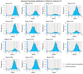
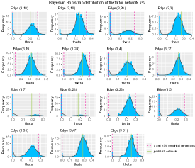
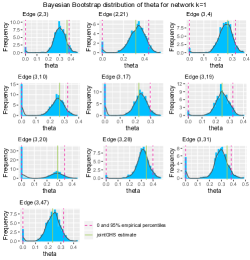
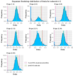
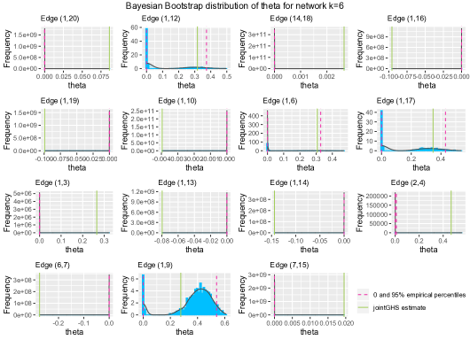
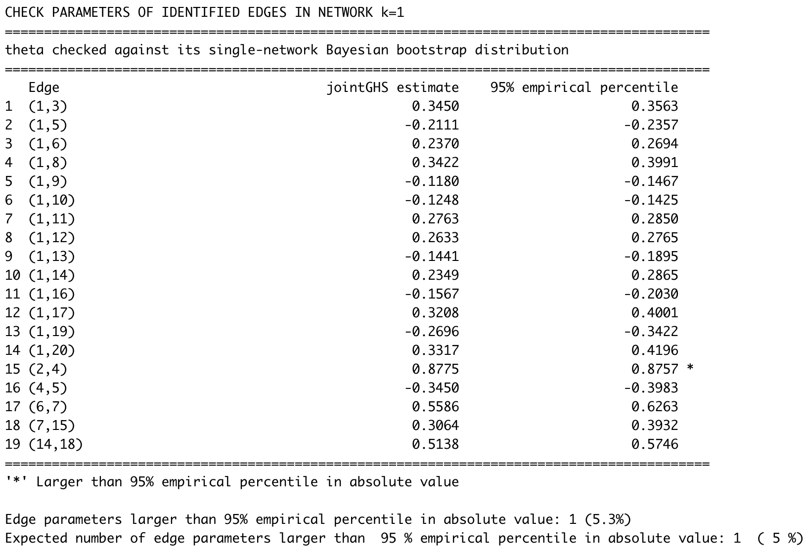
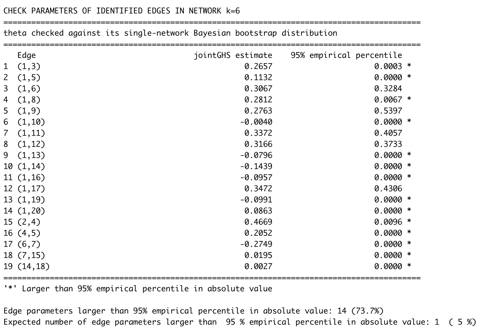
Appendix H Additional results
H.1 Extended simulation study
We have repeated the simulation study from the main manuscript with different numbers of networks , nodes and observations . Table H.5 shows the results for classes with nodes and , observations. As for the setting in the main manuscript, we observe that JGL tends to over-select edges severely and thus gets a low precision but high recall. Further, we again observe that SSJGL does not capture network-specific edges even for highly unrelated networks, leading to a decline in performance as network differences increase. Once again, GemBag does not appear to adapt to the similarity level of the networks, as the disagreement level of the inferred GemBag networks remains the same for all cases. Finally, we see that jointGHS adapts well to the varying sparsity levels, with the method performing similar to SSJGL for highly related networks and outperforming it for less similar networks.
Table H.6 shows the results for classes with nodes and , and observations. Notably, the average edge disagreement of the estimated networks that is displayed now only quantifies the amount of edges common to all networks, not pairs. Hence this number is higher for all methods. Otherwise we observe the same tendencies as in the previous setting, with JGL severely over-selecting edges, GemBag adapting little to varying disagreement levels and SSJGL having excellent performance for identical networks, but declining accuracy for less similar networks. We see that jointGHS appears to adapt well to the varying similarity levels.
| Disagr. | Method | Sparsity | Precision | Recall | Sparsity | Precision | Recall | |||
|---|---|---|---|---|---|---|---|---|---|---|
| 0 | JGL | 73 | 0.201 (0.005) | 0.08 (0.00) | 0.79 (0.03) | 0.161 (0.005) | 0.11 (0.01) | 0.85 (0.03) | ||
| GemBag | 43 | 0.020 (0.003) | 0.60 (0.06) | 0.60 (0.05) | 0.034 (0.006) | 0.42 (0.04) | 0.71 (0.04) | |||
| SSJGL | 0 | 0.009 (0.001) |
0.90 |
0.42 (0.04) | 0.009 (0.001) | 0.90 (0.06) | 0.42 (0.04) | |||
| jointGHS | 14 | 0.008 (0.000) |
0.86 |
0.35 (0.02) | 0.008 (0.000) |
0.95 |
0.36 (0.02) | |||
| 20 | JGL | 76 | 0.196 (0.009) | 0.08 (0.01) | 0.80 (0.04) | 0.151 (0.010) | 0.11 (0.01) | 0.81 (0.04) | ||
| GemBag | 54 | 0.021 (0.007) | 0.54 (0.09) | 0.54 (0.05) | 0.040 (0.016) | 0.37 (0.07) | 0.68 (0.05) | |||
| SSJGL | 0 | 0.007 (0.001) |
0.91 |
0.32 (0.03) | 0.007 (0.001) | 0.92 (0.05) | 0.32 (0.03) | |||
| jointGHS | 29 | 0.008 (0.001) | 0.79 (0.07) | 0.32 (0.02) | 0.006 (0.000) |
0.99 |
0.29 (0.02) | |||
| 40 | JGL | 77 | 0.199 (0.007) | 0.08 (0.01) | 0.79 (0.04) | 0.158 (0.007) | 0.10 (0.01) | 0.81 (0.03) | ||
| GemBag | 51 | 0.021 (0.006) | 0.52 (0.07) | 0.53 (0.04) | 0.037 (0.011) | 0.38 (0.06) | 0.67 (0.05) | |||
| SSJGL | 0 | 0.007 (0.001) |
0.89 |
0.31 (0.03) | 0.007 (0.001) | 0.90 (0.06) | 0.31 (0.03) | |||
| jointGHS | 30 | 0.008 (0.000) | 0.81 (0.06) | 0.33 (0.02) | 0.007 (0.000) |
0.96 |
0.34 (0.02) | |||
| 60 | JGL | 79 | 0.200 (0.007) | 0.08 (0.01) | 0.79 (0.04) | 0.159 (0.005) | 0.11 (0.01) | 0.84 (0.03) | ||
| GemBag | 45 | 0.022 (0.003) | 0.46 (0.05) | 0.50 (0.04) | 0.036 (0.006) | 0.38 (0.04) | 0.66 (0.03) | |||
| SSJGL | 0 | 0.006 (0.001) |
0.84 |
0.25 (0.03) | 0.006 (0.001) | 0.85 (0.06) | 0.26 (0.03) | |||
| jointGHS | 44 | 0.008 (0.001) |
0.77 |
0.32 (0.03) | 0.008 (0.000) |
0.93 |
0.35 (0.02) | |||
| 80 | JGL | 81 | 0.200 (0.007) | 0.08 (0.00) | 0.79 (0.04) | 0.156 (0.006) | 0.11 (0.01) | 0.84 (0.03) | ||
| GemBag | 48 | 0.022 (0.005) | 0.41 (0.05) | 0.45 (0.04) | 0.037 (0.01) | 0.36 (0.05) | 0.65 (0.05) | |||
| SSJGL | 1 | 0.005 (0.001) |
0.70 |
0.17 (0.02) | 0.005 (0.001) | 0.79 (0.08) | 0.19 (0.02) | |||
| jointGHS | 61 | 0.008 (0.001) |
0.72 |
0.29 (0.02) | 0.007 (0.000) |
0.94 |
0.32 (0.02) | |||
| 100 | JGL | 82 | 0.201 (0.005) | 0.08 (0.00) | 0.79 (0.04) | 0.156 (0.004) | 0.11 (0.00) | 0.89 (0.03) | ||
| GemBag | 45 | 0.023 (0.002) | 0.37 (0.04) | 0.42 (0.04) | 0.037 (0.002) | 0.36 (0.03) | 0.67 (0.04) | |||
| SSJGL | 1 | 0.005 (0.001) | 0.48 (0.08) | 0.11 (0.01) | 0.005 (0.001) | 0.65 (0.09) | 0.16 (0.02) | |||
| jointGHS | 72 | 0.008 (0.001) |
0.69 |
0.28 (0.03) | 0.006 (0.000) |
0.92 |
0.29 (0.02) | |||
| Disagr. | Method | Sparsity | Precision | Recall | Sparsity | Precision | Recall | Sparsity | Precision | Recall | ||||
|---|---|---|---|---|---|---|---|---|---|---|---|---|---|---|
| 0 | JGL | 92 | 0.201 (0.005) | 0.08 (0.00) | 0.79 (0.04) | 0.162 (0.005) | 0.11 (0.01) | 0.85 (0.04) | 0.182 (0.004) | 0.09 (0.00) | 0.82 (0.04) | |||
| GemBag | 70 | 0.020 (0.006) | 0.62 (0.08) | 0.59 (0.05) | 0.036 (0.009) | 0.42 (0.05) | 0.74 (0.05) | 0.026 (0.007) | 0.52 (0.07) | 0.64 (0.04) | ||||
| SSJGL | 33 | 0.010 (0.001) |
0.98 |
0.49 (0.04) | 0.010 (0.001) |
0.98 |
0.49 (0.04) | 0.010 (0.001) |
0.98 |
0.49 (0.04) | ||||
| jointGHS | 45 | 0.008 (0.000) | 0.87 (0.06) | 0.34 (0.03) | 0.007 (0.000) |
0.98 |
0.36 (0.02) | 0.008 (0.000) | 0.93 (0.05) | 0.35 (0.02) | ||||
| 20 | JGL | 94 | 0.197 (0.011) | 0.08 (0.01) | 0.79 (0.04) | 0.152 (0.014) | 0.11 (0.01) | 0.82 (0.03) | 0.181 (0.013) | 0.09 (0.01) | 0.80 (0.03) | |||
| GemBag | 74 | 0.018 (0.004) | 0.59 (0.07) | 0.53 (0.04) | 0.035 (0.011) | 0.39 (0.05) | 0.66 (0.05) | 0.023 (0.007) | 0.52 (0.07) | 0.57 (0.05) | ||||
| SSJGL | 35 | 0.008 (0.001) |
0.94 |
0.37 (0.03) | 0.008 (0.001) | 0.88 (0.05) | 0.34 (0.03) | 0.008 (0.001) | 0.88 (0.04) | 0.34 (0.03) | ||||
| jointGHS | 64 | 0.008 (0.001) | 0.80 (0.07) | 0.32 (0.03) | 0.006 (0.001) |
0.99 |
0.28 (0.03) | 0.007 (0.000) |
0.93 |
0.31 (0.02) | ||||
| 40 | JGL | 95 | 0.200 (0.005) | 0.08 (0.00) | 0.79 (0.04) | 0.159 (0.004) | 0.10 (0.00) | 0.81 (0.03) | 0.179 (0.005) | 0.09 (0.00) | 0.81 (0.03) | |||
| GemBag | 71 | 0.018 (0.001) | 0.56 (0.04) | 0.52 (0.04) | 0.033 (0.002) | 0.40 (0.03) | 0.66 (0.04) | 0.023 (0.002) | 0.49 (0.04) | 0.56 (0.04) | ||||
| SSJGL | 36 | 0.008 (0.001) |
0.88 |
0.34 (0.03) | 0.008 (0.001) | 0.87 (0.05) | 0.34 (0.03) | 0.008 (0.001) |
0.84 |
0.32 (0.03) | ||||
| jointGHS | 65 | 0.008 (0.001) | 0.80 (0.07) | 0.32 (0.02) | 0.007 (0.000) |
0.98 |
0.34 (0.02) | 0.008 (0.000) |
0.87 |
0.34 (0.02) | ||||
| 60 | JGL | 97 | 0.201 (0.005) | 0.08 (0.00) | 0.79 (0.04) | 0.161 (0.004) | 0.11 (0.00) | 0.85 (0.03) | 0.185 (0.004) | 0.09 (0.00) | 0.79 (0.04) | |||
| GemBag | 72 | 0.019 (0.002) | 0.51 (0.05) | 0.48 (0.04) | 0.034 (0.002) | 0.39 (0.03) | 0.66 (0.04) | 0.023 (0.002) | 0.46 (0.03) | 0.54 (0.03) | ||||
| SSJGL | 38 | 0.006 (0.001) |
0.84 |
0.26 (0.03) | 0.006 (0.001) | 0.76 (0.07) | 0.23 (0.02) | 0.006 (0.001) | 0.73 (0.06) | 0.22 (0.03) | ||||
| jointGHS | 82 | 0.008 (0.001) | 0.75 (0.07) | 0.30 (0.03) | 0.007 (0.000) |
0.92 |
0.34 (0.02) | 0.006 (0.000) |
0.92 |
0.29 (0.02) | ||||
| 80 | JGL | 97 | 0.200 (0.007) | 0.08 (0.01) | 0.78 (0.04) | 0.157 (0.007) | 0.11 (0.01) | 0.84 (0.04) | 0.185 (0.008) | 0.09 (0.01) | 0.79 (0.04) | |||
| GemBag | 73 | 0.019 (0.002) | 0.45 (0.04) | 0.43 (0.03) | 0.033 (0.002) | 0.39 (0.03) | 0.64 (0.04) | 0.024 (0.002) | 0.42 (0.03) | 0.50 (0.03) | ||||
| SSJGL | 39 | 0.005 (0.001) |
0.71 |
0.17 (0.02) | 0.005 (0.001) | 0.78 (0.07) | 0.19 (0.02) | 0.005 (0.001) | 0.69 (0.08) | 0.17 (0.02) | ||||
| jointGHS | 87 | 0.008 (0.001) |
0.72 |
0.29 (0.02) | 0.007 (0.000) |
0.95 |
0.32 (0.02) | 0.005 (0.001) |
0.94 |
0.25 (0.03) | ||||
| 100 | JGL | 98 | 0.200 (0.005) | 0.08 (0.00) | 0.78 (0.04) | 0.156 (0.004) | 0.11 (0.00) | 0.89 (0.03) | 0.178 (0.005) | 0.10 (0.00) | 0.88 (0.04) | |||
| GemBag | 76 | 0.025 (0.002) | 0.37 (0.04) | 0.45 (0.04) | 0.039 (0.003) | 0.34 (0.03) | 0.67 (0.04) | 0.032 (0.002) | 0.38 (0.03) | 0.61 (0.04) | ||||
| SSJGL | 38 | 0.007 (0.001) | 0.40 (0.07) | 0.13 (0.02) | 0.007 (0.001) | 0.44 (0.06) | 0.15 (0.02) | 0.007 (0.001) | 0.45 (0.06) | 0.15 (0.02) | ||||
| jointGHS | 98 | 0.008 (0.001) |
0.66 |
0.27 (0.03) | 0.006 (0.000) |
0.93 |
0.29 (0.02) | 0.006 (0.001) |
0.83 |
0.27 (0.02) | ||||
H.2 Threshold-free comparison
H.2.1 Precision-recall curves
To allow for a threshold-free comparison, we have created precision-recall curves. The curves show the precision plotted against the recall, and illustrates the trade-off between the two measures. A challenge when creating these curves is the tendency of the joint graphical horseshoe to do sparse edge selection, where the number of selected edges halts for sufficiently large values of the global shrinkage parameter . Further, because the ECM estimator sets precision matrix elements to be either zero (by machine precision) or clearly non-zero, thresholding partial correlation magnitudes does not allow us to exceed the number of edges selected by jointGHS. In our simulations, this means that we can not get jointGHS to exceed recall . To make a fair comparison, we thus create cut-off precision-recall curves.
To vary the number of selected edges, and thus the precision and recall, we vary the penalty parameter in JGL and the effective penalty parameter in SSJGL, as suggested by Li et al. [2019b]. To decrease the number of selected edges in jointGHS, we threshold the estimated partial correlations. In GemBag we vary the threshold for the estimated inclusion probabilities, as suggested by Yang et al. [2021]. Notably, with many edges being given the same edge inclusion probabilities, in this simulation GemBag tends to give relatively large recalls () outside of our comparison range. When we threshold so that only edges with inclusion probabilities equal to 1 are included, we get only one point within the interval with recall around . Thresholding by partial correlation magnitude leads to the same problem. Thus, a fair precision-recall curve comparison with GemBag is difficult as it does not allow for sparse enough estimates. We therefore only display the few points corresponding to Gembag in the interval, but do not connect them by line or calculate the area under the curve.
We consider the same settings as in our comparative simulation study; all with graphs and either or nodes, with various similarity of the true graph structures. For nodes, we reconstruct networks from and observations, and for nodes we reconstruct networks from and observations. The results for nodes are shown in Figure H.18 and the results for nodes are shown in Figure H.19.
As we see, the precision of the sparse jointGHS estimates remain very high in all cases. The cut-off where the recall is around is exactly when jointGHS does not allow for further edge inclusion as it does not find sufficient evidence for additional edges. This is a benefit the method has in this comparison, and it should be kept in mind when noting that it outperforms the other methods in all cases. It is however evident that if sparse edge selection with very high confidence in the selected edges is desired, jointGHS is the most suitable. The other methods appear to be more suitable if one is more interested in capturing as many of the true edges as possible, and is not as concerned about false positives.
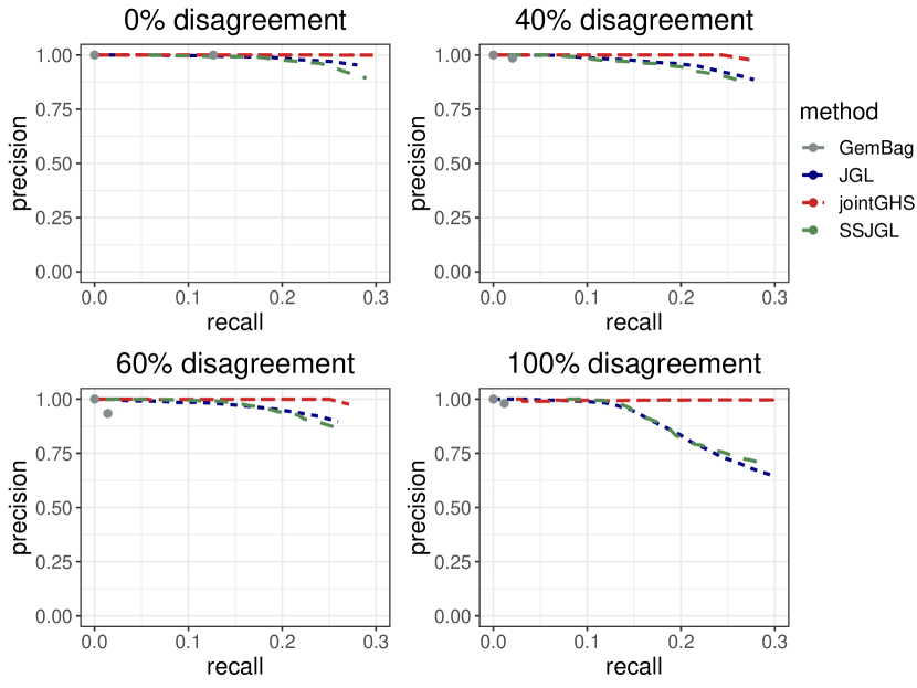
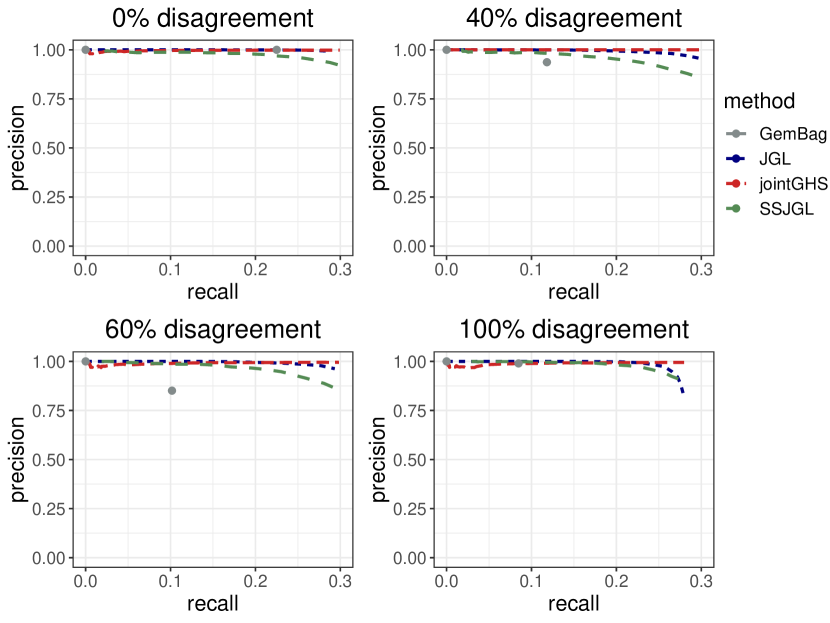
H.2.2 AUPRC
We have also calculated the cut-off area under the precision-recall curves (AUPRC), i.e. the area under the curves up to . We denote this the . The closer the is to , the better the estimation accuracy with fewer false positives. The results are shown in Table H.7. We observe that the jointGHS had either one of the highest or the highest scores in all settings, with values very close to , implying almost no false positives. The other methods also have high scores, though their scores decline more as the network disagreement increases. Again, it is evident that jointGHS is the most suitable for sparse edge selection where high confidence in the selected edges is important, while the others are more suitable for selecting more edges at the cost of lower precision.
| Disagr. | Method | ||||
|---|---|---|---|---|---|
| 0 | JGL | 0.295 |
0.300 |
||
| SSJGL | 0.292 | 0.293 | |||
| jointGHS |
0.300 |
0.299 |
|||
| 40 | JGL | 0.287 | 0.297 | ||
| SSJGL | 0.286 | 0.287 | |||
| jointGHS |
0.299 |
0.300 |
|||
| 60 | JGL | 0.285 |
0.298 |
||
| SSJGL | 0.285 | 0.289 | |||
| jointGHS |
0.299 |
0.297 |
|||
| 100 | JGL | 0.263 | 0.284 | ||
| SSJGL | 0.267 | 0.292 | |||
| jointGHS |
0.299 |
0.296 |
|||
H.3 Scalability
H.3.1 Scalability of single network inference with fastGHS
Figure H.20 shows the CPU time used to infer a network for various numbers of nodes, for fastGHS.
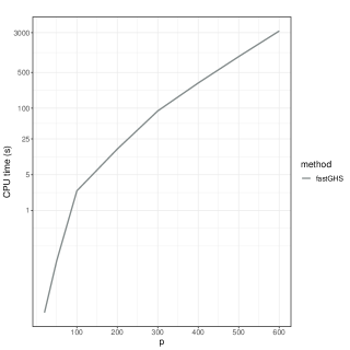
H.3.2 Scalability of multiple network inference with jointGHS
Figure H.21 shows the CPU time used to infer networks with jointGHS for various numbers of nodes.