Abstract

We study probes of neutral triple gauge couplings (nTGCs) at the LHC and the proposed 100 TeV $pp$ colliders, and compare their sensitivity reaches with those of the proposed $e^{+}e^{-}$ colliders. The nTGCs provide a unique window to the new physics beyond the Standard Model (SM) because they can arise from SM effective field theory (SMEFT) operators that respect the full electroweak gauge group $\mathrm{SU(2)}_{\mathrm{L}}\!\otimes\mathrm{U(1)}_{\mathrm{Y}}$ of the SM only at the level of dimension-8 or higher. We derive the neutral triple gauge vertices (nTGVs) generated by these dimension-8 operators in the broken phase and map them onto a newly generalized form factor formulation, which takes into account only the residual U(1)_em gauge symmetry. Using this mapping, we derive new relations between the form factors that guarantee a truly consistent form factor formulation of the nTGVs and remove large unphysical energy-dependent terms. We then analyze the sensitivity reaches of the LHC and future 100 TeV hadron colliders for probing the nTGCs via both the dimension-8 nTGC operators and the corresponding nTGC form factors in the reaction $\hskip 0.85358ptp{\hskip 0.85358pt}p{\hskip 0.85358pt}(q{\hskip 0.85358pt}\bar{q})\!\rightarrow\!Z\gamma\hskip 0.85358pt$ with $Z\!\rightarrow\!\ell^{+}\ell^{-}\!,\hskip 0.85358pt\nu{\hskip 0.85358pt}\bar{\nu}{\hskip 0.85358pt}\hskip 0.85358pt$. We compare their sensitivities with the existing LHC measurements of nTGCs and with those of the high-energy $e^{+}e^{-}$ colliders. In general, we find that the prospective LHC sensitivities are comparable to those of an $e^{+}e^{-}$ collider with center-of-mass energy $\leqslant\!1$ TeV, whereas an $e^{+}e^{-}$ collider with center-of-mass energy $(3-5)$ TeV would have greater sensitivities, and a 100 TeV $pp$ collider could provide the most sensitive probes of the nTGCs.

( Phys. Rev. D in press, Editors’ Suggestion )

1 Introduction

Neutral triple-gauge couplings (nTGCs) provide a unique window for probing the new physics beyond the Standard Model (SM). It is well known that they do not appear among the dimension-4 terms of the SM Lagrangian, nor are they generated by dimension-6 terms in its extension to the Standard Model Effective Field Theory (SMEFT) [1]. Instead, the nTGCs first appear through the gauge-invariant dimension-8 operators [2]-[6] in the SMEFT. Hence any indication of a non-vanishing nTGC would be direct prima facie evidence for new physics beyond the SM, which is different in nature from anything that might be first revealed by dimension-6 operators of the SMEFT [7]-[9]. Moreover, searching for the effects of interference between the other dimension-8 interactions and the SM contributions to amplitudes must contend with possible contributions that are quadratic in dimension-6 interactions, which is not an issue for the nTGCs.

Relatively few experimental probes of dimension-8 SMEFT interactions have been proposed in the literature. One of them is the nTGCs mentioned above [2]-[6], which first arise from the dimension-8 operators of the SMEFT and have no counterpart in the SM Lagrangian of dimension-4 or in the dimension-6 SMEFT interactions. Recent works have studied how the nTGCs can be probed by measuring $Z\gamma$ production at high-energy $e^{+}e^{-}$ colliders [5][6][10] and $pp$ colliders [11] under planning. Other examples include light-by-light scattering [12], which has been measured at the LHC and could also be interesting for high-energy $e^{+}e^{-}$ colliders [13], and the processes gluon$\hskip 0.85358pt+\hskip 0.85358pt$gluon $\!\rightarrow\!\gamma+\gamma$ [14] and gluon$\hskip 0.85358pt+\hskip 0.85358pt$gluon $\!\rightarrow\!Z+\gamma$ [15], which have been probed at the LHC. There are also recent studies on the dimension-8 operators induced by top-like heavy vector quarks and the their probes via $t\bar{t}h$ production at hadron colliders [16], and on the dimension-8 operators induced by the heavy Higgs doublet of the two-Higgs-doublet model [17].

In this work, we present a systematic study of the sensitivity reaches of probing the dimension-8 nTGC interactions by measuring $Z\gamma$ production at the LHC (13 TeV) and the $pp\hskip 0.85358pt$(100 TeV) colliders. The nTGCs are coupling coefficients of the the neutral triple gauge vertices (nTGVs), which are often parametrized in terms of effective form factors that respect only the residual U(1)_em gauge symmetry of the electromagnetism. This is in contrast with the dimension-8 nTGC operators of the SMEFT, which respect the full electroweak gauge group $\text{SU(2)}_{\mathrm{L}}\!\otimes\text{U(1)}_{\mathrm{Y}}$ of the SM.  We derive the nTGVs from these dimension-8 operators in the broken phase and map them onto a newly generalized form factor formulation of the nTGVs. Using this mapping, we derive new nontrivial relations among the form factor parameters that ensure a truly consistent form factor formulation of the nTGVs and remove unphysically large energy-dependent terms. Using these, we analyze systematically the sensitivity reaches of the LHC and future hadron colliders for nTGC couplings via both the dimension-8 nTGC operators and the corresponding nTGC form factors. We also make a direct comparison of our LHC analysis with the existing LHC measurements of nTGCs in the reaction $\hskip 0.85358ptp{\hskip 0.85358pt}p{\hskip 0.85358pt}(q{\hskip 0.85358pt}\bar{q})\!\rightarrow\!Z\gamma\hskip 0.85358pt$ with $Z\!\!\rightarrow\!\nu{\hskip 0.85358pt}\bar{\nu}{\hskip 0.85358pt}\hskip 0.85358pt$ by the CMS [18] and ATLAS [19] collaborations based on the conventional nTGC form factor formulation that takes into account only the unbroken U(1)_em gauge symmetry [3][4]. From this comparison, we demonstrate the importance of using our proposed SMEFT form factor approach to analyze nTGC constraints at the LHC and future high-energy colliders.

The outline of this paper is as follows. In Section 2 we review the parametrization of nTGCs and derive the cross sections for the reaction $\,q\hskip 0.85358pt\bar{q}\!\rightarrow\!Z\gamma\,$ (followed by $Z\!\rightarrow\!f\bar{f}\hskip 0.85358pt$ decays) as induced by the nTGCs. We also analyze the perturbative unitarity bounds on the nTGCs, showing that they are much weaker than the collider limits we present in Sections 4-5. Then, in Section 3  we present a newly generalized form factor formulation of the nTGCs and demonstrate that the full spontaneously-broken electroweak gauge symmetry $\text{SU(2)}_{\mathrm{L}}\!\otimes\!\text{U(1)}_{\mathrm{Y}}$ of the SM leads to important restrictions on the nTGC form factors. As noted above, the full electroweak gauge symmetry is respected by the construction of the SMEFT, where the nTGCs appear first through dimension-8 operators. Using this formulation, we study in Section 4  the sensitivities of the LHC and future $pp\hskip 0.85358pt$(100 TeV) colliders for probes of the nTGCs in the reaction $pp{\hskip 0.85358pt}(q\bar{q}\!\rightarrow\!Z\gamma)$ with $Z\!\rightarrow\!\ell\hskip 0.85358pt\bar{\ell},\nu\hskip 0.85358pt\bar{\nu}\hskip 0.85358pt$. We make a direct comparison of the sensitivity bounds using our SMEFT formulation of nTGCs with the existing LHC measurements on the nTGCs. In Section 5, we further present a systematic comparison with the sensitivity reaches of the prospective high-energy $e^{+}e^{-}$ colliders. Finally, we summarize our findings and conclusions in Section 6.

2 Scattering Amplitudes and Cross Sections for nTGCs

In this section, we first set up the notations and present the dimension-8 operators for the neutral triple gauge couplings (nTGCs) and the corresponding neutral triple gauge vertices (nTGVs). Then, we derive the nTGC contributions to the $Z\gamma$ amplitudes and cross sections. Finally, we derive the perturbative unitarity constraints on the nTGC couplings.

2.1 nTGCs from the Dimension-8 Operators

In previous works [5][6] we studied the dimension-8 operators that generate nTGCs and for their contributions to helicity amplitudes and cross sections at $e^{+}e^{-}$ colliders. In particular, we identified a new set of CP-conserving pure gauge operators of dimension-8 for the nTGCs, one of which ($\mathcal{O}_{G+}$) can give leading contributions to the neutral triple gauge boson vertices $Z\gamma Z^{*}$ and $Z\gamma\gamma^{*}$ with enhanced energy-dependences $\propto\!E^{5}$. In this subsection, we recast them for our applications to the LHC and future high-energy $pp$ colliders.

The general dimension-8 SMEFT Lagrangian takes the following form:

$$\Delta\mathcal{L}(\text{dim-8})\,=\,\sum_{j}\frac{\tilde{c}_{j}}{\,\tilde{\Lambda}^{4}\,}\mathcal{O}_{j}\,=\,\sum_{j}\frac{\,\text{sign}(\tilde{c}_{j})\,}{\,\Lambda_{j}^{4}\,}\mathcal{O}_{j}\,=\,\sum_{j}\frac{1}{\,[\Lambda_{j}^{4}]\,}\mathcal{O}_{j}\,,$$ (2.1)

where the dimensionless coefficients $\,\tilde{c}_{j}$ are expected to be around ${O}(1)$ and may take either sign, $\,\text{sign}(\tilde{c}_{j})\!=\!\pm$ . For each dimension-8 operator $\mathcal{O}_{j}$ , we have defined in Eq.(2.1) the corresponding effective cutoff scale for new physics, $\,\Lambda_{j}\equiv\tilde{\Lambda}/|\tilde{c}_{j}|^{1/4}\,$. We also introduced a notation $\,[\Lambda_{j}^{4}]\equiv\mathrm{sign}(\tilde{c}_{j})\Lambda^{4}_{j}\hskip 0.85358pt$.

We have analyzed the following set of dimension-8 operators [5] that are relevant for our nTGC analysis:

$$g\mathcal{O}_{G+}\!\!\! = \!\!\widetilde{B}_{\!\mu\nu}W^{a\mu\rho}(D_{\rho}D_{\lambda}W^{a\nu\lambda}\!+\!D^{\nu}D^{\lambda}W^{a}_{\lambda\rho}),$$ (2.2a)

$$g\mathcal{O}_{G-}\!\!\! = \!\!\widetilde{B}_{\!\mu\nu}W^{a\mu\rho}(D_{\rho}D_{\lambda}W^{a\nu\lambda}\!-\!D^{\nu}D^{\lambda}W^{a}_{\lambda\rho}),$$ (2.2b)

$$\mathcal{O}_{\widetilde{B}W}\!\!\! = \!\!\mathrm{i}\,H^{\dagger}\widetilde{B}_{\mu\nu}W^{\mu\rho}\!\left\{D_{\rho},D^{\nu}\right\}\!H+\text{h.c.},$$ (2.2c)

$$\mathcal{O}_{\!C+}\!\!\! = \!\!\widetilde{B}_{\!\mu\nu}W^{a\mu\rho}\!\left[D_{\!\rho}(\overline{\psi_{\!L}}T^{a}\!\gamma^{\nu}\!\psi_{\!L})+D^{\nu}(\overline{\psi_{\!L}}T^{a}\!\gamma_{\rho}\psi_{\!L})\right]\!,$$ (2.2d)

$$\mathcal{O}_{\!C-}\!\!\! = \!\!\widetilde{B}_{\!\mu\nu}W^{a\mu\rho}\!\left[D_{\!\rho}(\overline{\psi_{\!L}}T^{a}\!\gamma^{\nu}\!\psi_{\!L})-D^{\nu}(\overline{\psi_{\!L}}T^{a}\!\gamma_{\rho}\psi_{\!L})\right]\!.$$ (2.2e)

The fermionic operators $\hskip 0.85358pt\mathcal{O}_{C+}$ and $\hskip 0.85358pt\mathcal{O}_{C-}\!$ do not contribute directly to the nTGC couplings, but are connected to the three bosonic nTGC operators $(\mathcal{O}_{G+},\hskip 0.85358pt\mathcal{O}_{G-},\hskip 0.85358pt\mathcal{O}_{\widetilde{B}W})$ by the equation of motion [5]:

$$\mathcal{O}_{C+}\!\!\! = \!\!\mathcal{O}_{G-}\!-\mathcal{O}_{\widetilde{B}W}\,,$$ (2.3a)

$$\mathcal{O}_{C-}\!\!\! = \!\!\mathcal{O}_{G+}-\{\,\mathrm{i}H^{\dagger}\widetilde{B}_{\mu\nu}{W}^{\mu\rho}\!\left[D_{\rho},D^{\nu}\right]\!H\!+\mathrm{i}\,2(D_{\rho}H)^{\!\dagger}\widetilde{B}_{\mu\nu}{W}^{\mu\rho}\!D^{\nu}H+\text{h.c.}\}\hskip 0.85358pt.\hskip 28.45274pt$$ (2.3b)

They both contribute to the quartic $\hskip 0.85358ptf\bar{f}Z\gamma\hskip 0.85358pt$ vertex and thus to the on-shell amplitude $\,\mathcal{T}[f\bar{f}\!\!\rightarrow\!\!Z\gamma\hskip 0.85358pt]\,$. Hence they can be probed by the reaction $f\bar{f}\!\rightarrow\!Z\gamma$ . However, we note that the operators $\mathcal{O}_{G+}$ and $\mathcal{O}_{C-}$ give exactly the same contribution to the on-shell amplitude $\,\mathcal{T}[f\bar{f}\!\rightarrow\!Z\gamma]\,$ at tree level [5], because Eq.(2.3b) shows that the difference $(\mathcal{O}_{C-}\!\!-\mathcal{O}_{G+})$ is given by the Higgs-doublet-related term on the right-hand side (RHS) which contains at least 4 gauge fields and is thus irrelevant for the amplitude $\,\mathcal{T}[f\bar{f}\!\rightarrow\!Z\gamma\hskip 0.85358pt]\,$ at the tree level.

We consider first the dimension-8 nTGC operators $\mathcal{O}_{G+},{\cal O}_{\widetilde{B}W}$ and $\mathcal{O}_{G-}$. These operators contribute to the $Z\gamma Z^{*}$ and $Z\gamma\gamma^{*}$ vertices as follows:

$$\Gamma_{Z\gamma Z^{*}(G+)}^{\alpha\beta\mu}(q_{1},q_{2},q_{3})\!\! = \!\!-\frac{\,v(q_{3}^{2}\!-\!M_{Z}^{2})\,}{\,M_{Z}\hskip 0.85358pt[\Lambda_{G+}^{4}]\,}\!\left(q_{3}^{2}\,q_{2\nu}\epsilon^{\alpha\beta\mu\nu}\!+2q_{2}^{\alpha}q_{3\nu}q_{2\sigma}\epsilon^{\beta\mu\nu\sigma}\right)\!,\hskip 45.5244pt$$ (2.4a)

$$\Gamma_{Z\gamma\gamma^{*}(G+)}^{\alpha\beta\mu}(q_{1},q_{2},q_{3})\!\! = \!\!-\frac{\,s_{W}v\,q_{3}^{2}\,}{\,c_{W}M_{Z}\hskip 0.85358pt[\Lambda_{G+}^{4}]\,}\!\left(q_{3}^{2}\,q_{2\nu}\epsilon^{\alpha\beta\mu\nu}\!+2q_{2}^{\alpha}q_{3\nu}q_{2\sigma}\epsilon^{\beta\mu\nu\sigma}\right)\!,\hskip 45.5244pt$$ (2.4b)

$$\hskip 45.5244pt\Gamma^{\alpha\beta\mu}_{Z\gamma Z^{*}\!(\widetilde{B}W)}({q}_{1},{q}_{2},{q}_{3})\!\! = \!\!\frac{\leavevmode\nobreak\ v\hskip 0.85358ptM_{Z}\hskip 0.85358pt({q}_{3}^{2}\!-\!M_{Z}^{2})\,}{\,[\Lambda_{\widetilde{B}W}^{4}]\,}\epsilon^{\alpha\beta\mu\nu}q_{2\nu}\,,$$ (2.4c)

$$\Gamma^{\alpha\beta\mu}_{Z\gamma\gamma^{*}(G-)}({q}_{1},{q}_{2},{q}_{3})\!\! = \!\!-\frac{\,s_{W}\hskip 0.85358ptv\hskip 0.85358ptM_{Z}\,}{\,c_{W}[\Lambda_{G-}^{4}]\,}\epsilon^{\alpha\beta\mu\nu}q_{2\nu}{q}_{3}^{2}\,.$$ (2.4d)

In the above and afterwards, the three gauge bosons are defined as outgoing.

We consider next the fermion-bilinear operator $\mathcal{O}_{C_{+}}$, which contributes to the effective contact vertex $q\bar{q}Z\gamma$ as follows:

$$\Gamma^{\alpha\beta}_{q\bar{q}Z\gamma(C+)}({q}_{1},{q}_{2})\,=\,-\text{sign}(\tilde{c}_{C+})\frac{\,2M_{Z}^{2}\hskip 0.85358ptT_{3}\,}{\,\Lambda^{4}\,}\epsilon^{\alpha\beta\mu\nu}q_{2\nu}\gamma_{\mu}P_{L}\,,$$ (2.5)

where the four external fields are on-shell. In the above formula, we have introduced the third component of the weak isospin $\,T_{3}\!=\pm\mbox{$\frac{\,{1}\,}{2}$}$  and the chirality projections $\hskip 0.85358ptP_{L(R)}\!=\!\mbox{$\frac{\,{1}\,}{2}$}(1\!\mp\!\gamma_{5})\hskip 0.85358pt$.

2.2 nTGC Contributions to $Z\gamma$ Amplitude and Cross Section

Next, we study the helicity amplitude for the quark and antiquark annihilation process $\,q\hskip 0.85358pt\bar{q}\!\rightarrow\!Z\gamma\hskip 0.85358pt$,  where the quark has weak isospin $\hskip 0.85358ptT_{3}\hskip 0.85358pt$ and electric charge $\hskip 0.85358ptQ\hskip 0.85358pt$. We can compute the SM contributions to the helicity amplitude of $\,q\hskip 0.85358pt\bar{q}\!\rightarrow\!Z(\lambda)\gamma(\lambda^{\prime})\,$ as follows:

$$\mathcal{T}_{\text{sm}}^{ss^{\prime}\!,\text{T}}\!\!\left\lgroup\!\!\!\begin{array}[]{cc}--\!&\!-+\\ +-\!&\!++\\ \end{array}\!\!\right\rgroup\!\! = \!\!\!\frac{-2\hskip 0.85358pte^{2}Q}{\,s_{W}c_{W}(s\!-\!M_{Z}^{2})\,}\!\!\!\left\lgroup\!\!\!\!\begin{array}[]{ll}\left(c_{L}^{\prime}\!\cot\!\frac{\theta}{2}\!-\!c_{R}^{\prime}\!\tan\!\frac{\theta}{2}\right)\!M_{Z}^{2}\leavevmode\nobreak\ \!&\!\!\left(-c_{L}^{\prime}\!\cot\!\frac{\theta}{2}\!+\!c_{R}^{\prime}\!\tan\!\frac{\theta}{2}\right)\!s\\[5.69054pt] \left(c_{L}^{\prime}\!\tan\!\frac{\theta}{2}\!-\!c_{R}^{\prime}\!\cot\!\frac{\theta}{2}\right)\!s\!&\!\!\left(-c_{L}\!\tan\!\frac{\theta}{2}\!+\!c_{R}\!\cot\!\frac{\theta}{2}\right)\!M_{Z}^{2}\end{array}\!\!\!\right\rgroup\!\!,\hskip 39.83385pt$$ (2.6e)

$$\mathcal{T}_{\text{sm}}^{ss^{\prime}\!,\text{L}}(0-,0+)\!\!\! = \!\!\!\frac{\,-2\sqrt{2}\hskip 0.85358pte^{2}Q\hskip 0.85358pt(c_{L}^{\prime}\!\!+\!c_{R}^{\prime})\hskip 0.85358ptM_{Z}\sqrt{s\,}\leavevmode\nobreak\ }{\,s_{W}c_{W}(s\!-\!M_{Z}^{2})\,}\left(1,\,-1\right),$$ (2.6f)

for the helicity combinations $\lambda\lambda^{\prime}\!=\!(--,-+,+-,++)$ and $\lambda\lambda^{\prime}\!=\!(0-,0+)$. In the above, we have defined the coupling coefficients $\,(c_{L}^{\prime},\,c_{R}^{\prime})=((T_{3}-Qs_{W}^{2})\delta_{\!s,-\frac{1}{2}},\hskip 0.85358pt-Qs_{W}^{2}\delta_{\!s,\frac{1}{2}})$  with the notations $\,(s_{W},\,c_{W})=(\sin\theta_{W},\hskip 0.85358pt\cos\theta_{W})\,$ and the subscript index $\,s=\mp\frac{1}{2}$  denoting the initial-state fermion helicities. If the initial-state quark and antiquark masses are negligible, the relation $\hskip 0.85358pts=-s^{\prime}\hskip 0.85358pt$ holds.

We find the following contributions to the corresponding helicity amplitudes from the dimension-8 operator $\mathcal{O}_{\!G+}\,(\mathcal{O}_{\!C-})$:

$$\mathcal{T}_{(8),{G+}}^{ss^{\prime}\!,\text{T}}\!\!\left\lgroup\!\!\!\begin{array}[]{cc}--\!&\!-+\\ +-\!&\!++\\ \end{array}\!\!\!\right\rgroup\!\! = \!\!\!\frac{\,(c^{\prime}_{L}\!\!+\!c^{\prime}_{R})(s\!-\!M_{Z}^{2})\hskip 0.85358pts\sin\!\theta\leavevmode\nobreak\ }{[\Lambda_{G+}^{4}]}\!\!\left\lgroup\!\!\begin{array}[]{cc}1&0\\[2.84526pt] 0&-1\end{array}\!\!\right\rgroup\!\!,$$ (2.7e)

$$\mathcal{T}_{(8),{G+}}^{ss^{\prime}\!,\text{L}}(0-,0+)\!\!\! = \!\!\!\frac{\,\sqrt{2}M_{Z}(s\!-\!M_{Z}^{2})\sqrt{s\,}\,}{[\Lambda_{G+}^{4}]}\!\left(\!c^{\prime}_{L}\!\sin^{2}\!\frac{\theta}{2}\!-c^{\prime}_{R}\!\cos^{2}\!\frac{\theta}{2},\leavevmode\nobreak\ c^{\prime}_{R}\!\sin^{2}\!\frac{\theta}{2}\!-c^{\prime}_{L}\!\cos^{2}\!\frac{\theta}{2}\right)\!,\hskip 51.21495pt$$ (2.7f)

where the coupling coefficients are given by $\,(c^{\prime}_{L},\,c^{\prime}_{R})\!=\!-T_{3}(\delta_{\!s,-\frac{1}{2}},\,0)$, and we have used the notations $\,[\Lambda_{G+}^{4}]\equiv\mathrm{sign}(\tilde{c}_{G+})\Lambda^{4}_{G+}$ for $\mathcal{O}_{G+}\hskip 0.85358pt$. We note that in Eq.(2.7e) the off-diagonal amplitudes vanish exactly. This is because the final state $Z(\lambda)\gamma(\lambda^{\prime})$ with helicities $\lambda\lambda^{\prime}\!=\!+-,-+\hskip 0.85358pt$ should have their spin angular momenta pointing to the same direction in their central-of-mass frame and thus the sum of their spin momenta would have magnitude equal $2\hskip 0.85358pt$. But this is disallowed by the $s$-channel spin-1 gauge boson $Z^{*}$ or $\gamma^{*}$.  For the same reason, the off-diagonal amplitudes contributed by the other dimension-8 operators in the following Eq.(2.8e) have to vanish as well.

As for the other three dimension-8 operators $(\mathcal{O}_{G-},\hskip 0.85358pt\mathcal{O}_{\tilde{B}W},\hskip 0.85358pt\mathcal{O}_{C+})$, we derive their contributions to the helicity amplitudes of the reaction $\,q\hskip 0.85358pt\bar{q}\!\rightarrow\!Z\gamma\,$ as follows:

$$\mathcal{T}_{(8),j}^{ss^{\prime}\!,\text{T}}\!\!\left\lgroup\!\!\begin{array}[]{cc}--\!&\!-+\\ +-\!&\!++\\ \end{array}\!\!\right\rgroup\!\!\!\! = \!\!\!\frac{\,(c^{\prime}_{L}\!+c^{\prime}_{R})\sin\!\theta\hskip 0.85358ptM_{Z}^{2}\hskip 0.85358pt(s\!-\!M_{Z}^{2})\,}{[\Lambda_{j}^{4}]}\!\!\left\lgroup\!\!\begin{array}[]{cr}1\!&0\\[2.84526pt] 0\!&-1\end{array}\!\!\right\rgroup\!\!,$$ (2.8e)

$$\mathcal{T}_{(8),j}^{ss^{\prime}\!,\text{L}}(0-,0+)\!\! = \!\!\!\frac{\,\sqrt{2\,}M_{Z}(s\!-\!M_{Z}^{2})\sqrt{s}\,}{[\Lambda_{j}^{4}]}\!\left(\!c^{\prime}_{L}\!\sin^{2}\!\frac{\theta}{2}\!-c^{\prime}_{R}\!\cos^{2}\!\frac{\theta}{2},\leavevmode\nobreak\ c^{\prime}_{R}\!\sin^{2}\!\frac{\theta}{2}\!-c^{\prime}_{L}\!\cos^{2}\!\frac{\theta}{2}\right)\!,\hskip 39.83385pt$$ (2.8f)

where $\,[\Lambda_{j}^{4}]\!=\mathrm{sign}(\tilde{c}_{j})\Lambda_{j}^{4}\,$ and $\,j\!\in\!({G_{-}},\hskip 0.85358pt{\widetilde{B}W},\hskip 0.85358pt{C_{+}})\hskip 0.85358pt$.  In Eq.(2.8), the coupling factors $\,(c^{\prime}_{L},\,c^{\prime}_{R})$ are given by

$$(c^{\prime}_{L},\,c^{\prime}_{R}) \,=\,-Qs_{W}^{2}(\delta_{\!s,-\frac{1}{2}},\,\delta_{\!s,\frac{1}{2}})\hskip 0.85358pt, (\hskip 0.85358pt\text{for}\leavevmode\nobreak\ \mathcal{O}_{G-}\hskip 0.85358pt)\hskip 0.85358pt,$$ (2.9a)

$$(c^{\prime}_{L},\,c^{\prime}_{R}) \,=\,\big{(}q_{L}\delta_{\!s,-\frac{1}{2}},\,q_{R}\hskip 0.85358pt\delta_{\!s,\frac{1}{2}}\big{)}\hskip 0.85358pt, (\hskip 0.85358pt\text{for}\leavevmode\nobreak\ \mathcal{O}_{\!\widetilde{B}W}\hskip 0.85358pt)\hskip 0.85358pt,$$ (2.9b)

$$(c^{\prime}_{L},\,c^{\prime}_{R}) \,=\,-T_{3}(\delta_{\!s,-\frac{1}{2}},\,0)\hskip 0.85358pt, (\hskip 0.85358pt\text{for}\leavevmode\nobreak\ \mathcal{O}_{C+}\hskip 0.85358pt)\hskip 0.85358pt,$$ (2.9c)

and the coefficients $\,(q_{L},\,q_{R})\!=\!(T_{3}\!-\!Qs_{W}^{2},\,-Qs_{W}^{2})$ arise from $Z$ gauge boson couplings with the (left, right)-handed the quarks.

The kinematics for the complete annihilation process $\hskip 0.85358ptq\hskip 0.85358pt\bar{q}\rightarrow Z\gamma\!\rightarrow\!f\bar{f}\gamma\hskip 0.85358pt$ are defined by the three angles $(\theta,\,\theta_{*},\,\phi_{*})$, where $\,\theta\,$ is the polar scattering angle between the direction of the outgoing $Z$ and the initial state quark $\hskip 0.85358ptq\hskip 0.85358pt$, $\,\theta_{*}$ denotes the angle between the direction opposite to the final-state $\gamma$ and the final-state fermion $f$ direction in the $Z$ rest frame, and $\,\phi_{*}\,$ is the angle between the scattering plane and the decay plane of $Z$ in the $\hskip 0.85358ptq\hskip 0.85358pt\bar{q}\hskip 0.85358pt$ center-of-mass frame [cf. Eq.(4.8)]. We note that, at a $pp$ collider, we cannot determine which is the initial state quark (antiquark) in each collision, so we could only determine the scattering angle up to an ambiguity $\theta\leftrightarrow\pi-\theta\hskip 0.85358pt$. It follows that the determination of the angle between the scattering plane and $Z$-decay plane also has an ambiguity $\hskip 0.85358pt\phi_{*}\leftrightarrow\hskip 0.85358pt\pi-\phi_{*}\hskip 0.85358pt$.

Taking these remarks into account, we can express the full amplitude of the reaction process $\hskip 0.85358ptq\hskip 0.85358pt\bar{q}\rightarrow Z\gamma\!\rightarrow\!f\bar{f}\gamma\hskip 0.85358pt$ in the following form:

$$\mathcal{T}^{ss^{\prime}}_{\sigma\sigma^{\prime}\!\lambda}\!(f\bar{f}\gamma) \!\!=\!\! \frac{\,eM_{Z}\mathcal{D}_{Z}\,}{s_{W}c_{W}}\left[\sqrt{2\,}e^{\mathrm{i}\phi_{*}}\!\left(\!f_{R}^{\sigma}\cos^{2}\!\frac{\,\theta_{*}}{2}\!-f_{L}^{\sigma}\!\sin^{2}\!\frac{\,\theta_{*}}{2}\!\right)\!\mathcal{T}_{ss^{\prime}}^{T}(+\lambda)\right.$$ (2.10)

$$\hskip 28.45274pt\left.+\sqrt{2\,}e^{-i\phi_{*}}\!\left(\!f_{R}^{\sigma}\sin^{2}\!\frac{\,\theta_{*}}{2}\!-f_{L}^{\sigma}\!\cos^{2}\!\frac{\,\theta_{*}}{2}\!\right)\!\mathcal{T}_{ss^{\prime}}^{T}(-\lambda)+(f_{R}^{\sigma}\!+\!f_{L}^{\sigma})\sin\!\theta_{*}\mathcal{T}_{ss^{\prime}}^{L}(0\lambda)\right]\!,\hskip 8.53581pt$$

where $\,\mathcal{D}_{Z}=1/(q_{1}^{2}\!-\!M_{Z}^{2}+\mathrm{i}\hskip 0.85358ptM_{Z}\Gamma_{Z})\,$ comes from the $Z$ propagator. In Eq.(2.10), the final-state fermions have the electroweak gauge couplings given by $\hskip 0.85358pt(f_{L}^{\sigma},f_{R}^{\sigma})\!=\!((T_{3}-Qs_{W}^{2})\hskip 0.85358pt\delta_{\!\sigma,-\frac{1}{2}},\hskip 0.85358pt-Qs_{W}^{2}\delta_{\!\sigma,\frac{1}{2}})\hskip 0.85358pt$, and the scattering amplitudes $\mathcal{T}_{ss^{\prime}}^{T}(\pm\lambda)$ and $\mathcal{T}_{ss^{\prime}}^{L}(0\lambda)$ represent the on-shell helicity amplitudes for the reaction $\hskip 0.85358ptq\hskip 0.85358pt\bar{q}\!\rightarrow Z\gamma$ :

$$\mathcal{T}_{ss^{\prime}}^{T}(\pm\lambda)\!\! = \!\!\mathcal{T}^{ss^{\prime}\!,T}_{\text{sm}}(\pm\lambda)+\mathcal{T}^{ss^{\prime}\!,T}_{(8)}(\pm\lambda)\hskip 0.85358pt,$$

$$\mathcal{T}_{ss^{\prime}}^{L}(0\lambda)\!\! = \!\!\mathcal{T}^{ss^{\prime}\!,L}_{\text{sm}}(0\lambda)+\mathcal{T}^{ss^{\prime}\!,L}_{(8)}(0\lambda)\hskip 0.85358pt,$$

which receive contributions from both the SM and the dimension-8 operator.

Applying a lower angular cut $\,\sin\theta\!>\!\sin\delta\,$ for some $\delta\!\ll\!1$, we derive the following total cross section for the partonic process $\,q\hskip 0.85358pt\bar{q}\!\rightarrow\!Z\gamma\hskip 0.85358pt$,  including both the linear and quadratic contributions of $\mathcal{O}_{G+}$ and summing over the final-state $Z$ and $\gamma$ polarizations:

$$\sigma(Z\gamma)\!\! = \!\!\frac{\,e^{4}(q_{L}^{2}\!+\!q_{R}^{2})\hskip 0.85358ptQ^{2}\!\left[-(s\!-\!M^{2}_{Z})^{2}\!-\!2(s^{2}\!+\!M_{Z}^{4})\ln\sin\!\frac{\delta}{2}\,\right]\,}{\,8\pi s_{W}^{2}c_{W}^{2}(s\!-\!M^{2}_{Z})s^{2}\,}\hskip 42.67912pt$$

$$\!\!+\,\frac{\,e^{2}q_{L}Q\hskip 0.85358pt{T_{3}}M_{Z}^{2}\!\left(s\!-\!M_{Z}^{2}\right)\,}{4\pi s_{W}c_{W}s}\frac{1}{\,[\Lambda_{G+}^{4}]\,}$$

$$\!\!+\,\frac{\leavevmode\nobreak\ {T_{3}^{2}}\hskip 0.85358pt(s+\!M_{Z}^{2})\!\left(s\!-\!M^{2}_{Z}\right)^{\!3}\,}{\,48\pi\,s\,}\frac{1}{\,\Lambda_{G+}^{8}\,}+O(\delta)\,,$$

where the weak isospin $\,T_{3}=\pm\mbox{$\frac{\,{1}\,}{2}$}\,$ is associated with the $\,W_{3}\hskip 0.85358pt$ gauge coupling, and the coefficients $\,(q_{L},\,q_{R})\!=\!(T_{3}-Qs_{W}^{2},\,-Qs_{W}^{2})$ are the (left, right)-handed gauge couplings of the quarks to the $Z$ boson. In Eq.(2.2), $\sqrt{s\,}\hskip 0.85358pt$ denotes the center-of-mass energy of the partonic process $\,q\hskip 0.85358pt\bar{q}\!\rightarrow Z\gamma\hskip 0.85358pt$, but for the $pp$ collider analyses in Section 4 we will rename the above partonic center-of-mass energy as $\sqrt{\hat{s}\,}$ for clarity.

We define the normalized angular distribution functions as follows:

$$f_{\xi}^{j}\,=\,\frac{1}{\sigma_{\!j}}\frac{\mathrm{d}\sigma_{\!j}}{\,\mathrm{d}\xi\,}\,,$$ (2.13)

where the angles $\,\xi\in(\theta,\,\theta_{*},\,\phi_{*})$,  and the cross sections $\,\sigma_{j}$ ($j=0,1,2$) represent the SM contribution ($\sigma_{0}$), the ${O}(\Lambda^{-4})$ contribution ($\sigma_{1}$), and the ${O}(\Lambda^{-8})$ contribution ($\sigma_{2}$),  respectively. In the following, we derive the explicit formulas for the normalized azimuthal angular distribution functions $\,f_{\phi_{*}}^{j}\,$:

$$f_{\phi_{*}}^{0}\!\!\!\! = \!\!\!\!\frac{1}{\,2\pi\,}+\frac{\,3\pi^{2}(q_{L}^{2}\!-\!q_{R}^{2})(f_{L}^{2}\!-\!f_{R}^{2})M_{Z}\sqrt{s}\,(s\!+\!M_{Z}^{2})\cos\phi_{*}\!-8(q_{L}^{2}\!+\!q_{R}^{2})(f_{L}^{2}\!+\!f_{R}^{2})M_{Z}^{2}\,s\cos 2\phi_{*}\,}{\,16\pi(q_{L}^{2}\!+\!q_{R}^{2})(f_{L}^{2}+f_{R}^{2})\!\left[(s\!-\!M_{Z}^{2})^{2}\!+2(s^{2}\!+\!M_{Z}^{4})\ln\sin\!\frac{\delta}{2}\hskip 0.85358pt\right]\,}+O(\delta),\hskip 5.69054pt$$

$$f_{\phi_{*}}^{1}\!\!\!\! = \!\!\!\!\frac{1}{\,2\pi\,}-\frac{\,3\pi(f_{L}^{2}\!-\!f_{R}^{2})(M_{Z}^{2}+5\hskip 0.85358pts)\cos\phi_{*}\,}{256(f_{L}^{2}\!+\!f_{R}^{2})M_{Z}\sqrt{s}}+\frac{\,s\cos 2\phi_{*}\,}{8\pi M_{Z}^{2}}\,,$$ (2.14b)

$$f_{\phi_{*}}^{2}\!\!\!\! = \!\!\!\!\frac{1}{\,2\pi\,}-\frac{\,9\pi(f_{L}^{2}\!-\!f_{R}^{2})M_{Z}\sqrt{s\,}\cos\phi_{*}\,}{\,128(f_{L}^{2}\!+\!f_{R}^{2})(s\!+\!M_{Z}^{2})\,}\,,$$ (2.14c)

where we denote the $Z$ couplings with the initial state quarks as $\,(q_{L},\,q_{R})\!=\!(T_{3}-Qs_{W}^{2},\hskip 0.85358pt-Qs_{W}^{2})$, and the the $Z$ couplings with the final-state fermions as $\hskip 0.85358pt(f_{L},f_{R})\!=\!((T_{3}-Qs_{W}^{2}),\hskip 0.85358pt-Qs_{W}^{2})\hskip 0.85358pt$.

In the cases of the other nTGC operators $\mathcal{O}_{j}$, we further derive their contributions to the total cross sections of the reaction $\,q\hskip 0.85358pt\bar{q}\!\rightarrow Z\gamma\,$ as follows:

$$\sigma(Z\gamma) \!\!=\!\! \frac{\leavevmode\nobreak\ e^{4}(q_{L}^{2}\!+\!q_{R}^{2})Q^{2}\!\!\left[-(s\!-\!M^{2}_{Z})^{2}\!-\!2(s^{2}\!+\!M_{Z}^{4})\ln\sin\!\frac{\delta}{2}\,\right]\,}{\,8\pi s_{W}^{2}c_{W}^{2}(s\!-\!M^{2}_{Z})\hskip 0.85358pts^{2}\,}\hskip 42.67912pt$$

$$-\,\frac{\leavevmode\nobreak\ e^{2}Q(q_{L}x_{L}\!\!-\!q_{R}x_{R})M_{Z}^{2}\!\left(s\!-\!M_{Z}^{2}\right)\!\left(s\!+\!M^{2}_{Z}\right)\,}{\,8\pi s_{W}c_{W}\hskip 0.85358pts^{2}\,}\frac{1}{\,[\Lambda_{j}^{4}]\,}$$

$$+\frac{\leavevmode\nobreak\ (x_{L}^{2}\!+\!x_{R}^{2})M_{Z}^{2}\!\left(s\!+\!M^{2}_{Z}\right)\!\left(s\!-\!M^{2}_{Z}\right)^{\!3}\,}{\,48\pi\hskip 0.85358pts^{2}\,}\frac{1}{\,\Lambda_{j}^{8}\,}+O(\delta)\,,$$

where we define the relevant coupling coefficients $\hskip 0.85358pt(x_{L},\hskip 0.85358ptx_{R})\hskip 0.85358pt$ as

$$(x_{L},\,x_{R}) =-Qs_{W}^{2}(1,\,1), (\text{for}\leavevmode\nobreak\ \, \mathcal{O}_{j}=\mathcal{O}_{G-}),$$ (2.16a)

$$(x_{L},\,x_{R}) =\left(T_{3}\!-Qs_{W}^{2},\,-Qs_{W}^{2}\right)\!, (\text{for}\leavevmode\nobreak\ \, \mathcal{O}_{j}=\mathcal{O}_{\widetilde{B}W}),$$ (2.16b)

$$(x_{L},\,x_{R}) =-(T_{3},\,0), (\text{for}\leavevmode\nobreak\ \, \mathcal{O}_{j}=\mathcal{O}_{C+}).$$ (2.16c)

We see that in the high energy limit, the contributions of the SM, the interference term, and the squared term behave as $(s^{-1},\hskip 0.85358pts^{0},\hskip 0.85358pts^{2})$ respectively. We can compare the above cross section with that of Eq.(2.2) for the nTGC operator $\hskip 0.85358pt\mathcal{O}_{G+}$ where the SM term, the interference term, and the squared term scale as $(s^{-1},\hskip 0.85358pts^{0},\hskip 0.85358pts^{3})$ respectively. This shows that the contribution of $\hskip 0.85358pt\mathcal{O}_{G+}$ to the squared term has higher energy power enhancement of $\hskip 0.85358pts^{3}\hskip 0.85358pt$ than the factor $\hskip 0.85358pts^{2}\hskip 0.85358pt$ of the other operators.

Then, for the full process $\hskip 0.85358ptq\hskip 0.85358pt\bar{q}\!\rightarrow\!\!Z\gamma\!\!\rightarrow\!\!f\bar{f}\gamma\hskip 0.85358pt$, we further derive the following normalized angular distribution functions $\,f_{\phi_{*}}^{j}\,$ for the operators $(\mathcal{O}_{G-},\hskip 0.85358pt\mathcal{O}_{\widetilde{B}W},\hskip 0.85358pt\mathcal{O}_{C+})$:

$$f_{\phi_{*}}^{0}\!\!\! = \!\!\frac{1}{2\pi}+\frac{\,3\pi^{2}f_{-}^{2}q_{-}^{2}M_{Z}\sqrt{s}\,(s\!+\!M_{Z}^{2})\cos\!\phi_{*}\!-8f_{+}^{2}q_{+}^{2}M_{Z}^{2}\,s\cos\!2\phi_{*}\,}{\,16\pi f_{+}^{2}q_{+}^{2}\!\left[(s\!-\!M_{Z}^{2})^{2}\!+2(s^{2}\!+\!M_{Z}^{4})\ln\sin\frac{\delta}{2}\right]\,}+O(\delta),\hskip 11.38109pt$$ (2.17a)

$$f_{\phi_{*}}^{1}\!\!\! = \!\!\frac{1}{2\pi}-\frac{\,9\pi(q_{L}x_{L}\!+\!q_{R}x_{R})(f_{L}^{2}\!-\!f_{R}^{2})\sqrt{s}\,\cos\!\phi_{*}\,}{\,128(q_{L}x_{L}\!-\!q_{R}x_{R})(f_{L}^{2}\!+\!f_{R}^{2})M_{Z}\,}+\frac{s\cos\!2\phi_{*}\,}{\,4\pi(s\!+\!M_{Z}^{2})\,},$$ (2.17b)

$$f_{\phi_{*}}^{2}\!\!\! = \!\!\frac{1}{2\pi}-\frac{\,9\pi(x_{L}^{2}\!-\!x_{R}^{2})(f_{L}^{2}\!-\!f_{R}^{2})M_{Z}\sqrt{s}\,\cos\!\phi_{*}\,}{\,128(x_{L}^{2}\!+\!x_{R}^{2})(f_{L}^{2}\!+\!f_{R}^{2})(s\!+\!M_{Z}^{2})\,}\,,$$ (2.17c)

where we have defined the coefficients  $(f_{\pm}^{2},\,q_{\pm}^{2})\!\equiv\!(f_{L}^{2}\pm f_{R}^{2},\,q_{L}^{2}\pm q_{R}^{2})$, and the electroweak gauge couplings of the final state fermions are given by $\hskip 0.85358pt(f_{L},f_{R})\!=\!((T_{3}-Qs_{W}^{2}),\hskip 0.85358pt-Qs_{W}^{2})\hskip 0.85358pt$.

2.3 Analysis of Unitarity Constraints on nTGCs

In this subsection, we analyze the perturbative unitarity constraints on the nTGCs, showing that these constraints are much weaker than the sensitivity reaches of the collider probes presented in the following Sections 3-5.

We first make the following partial-wave expansion [20] of the nTGC contributions to the scattering amplitude for the reaction $f\bar{f}\!\rightarrow\!Z\gamma\hskip 0.85358pt$:

$$a_{J}\,=\,\frac{1}{\,32\pi\,}e^{i(\nu^{\prime}-\nu)\phi}\!\!\int_{-1}^{1}\!\!\text{d}(\cos\theta)\,d^{\hskip 0.85358ptJ}_{\nu^{\prime}\nu}(\cos\theta)\mathcal{T}_{\text{nTGC}}^{s_{f}s_{\bar{f}},\lambda_{Z}\lambda_{\gamma}},$$ (2.18)

where the differences of initial/final state helicities are given by $\,\nu\!=s_{f}\!-\!s_{\bar{f}}\!=\pm 1$ and $\,\nu^{\prime}\!=\lambda_{Z}\!-\!\lambda_{\gamma}\!=0,\pm 1\hskip 0.85358pt$, respectively. We note that for the present collider analysis it is sufficient to treat the initial-state fermions $(f,\bar{f})$ (light quarks or leptons) as massless. Thus we have $\,s_{f}\!=\!-s_{\bar{f}}\,$, which leads to $\,\nu=\!\pm 1\hskip 0.85358pt$. Hence the $\hskip 0.85358ptJ\!=\!1\hskip 0.85358pt$ partial wave makes the leading contribution. The relevant Wigner $d$ functions are given by

$$d^{1}_{1,0}=-\mbox{$\frac{\,{1}\,}{\,\sqrt{2\,}\,}$}\sin\theta\hskip 0.85358pt,\hskip 22.76219ptd^{1}_{1,\pm 1}=\mbox{$\frac{\,{1}\,}{\,2\,}$}(1\pm\cos\theta)\hskip 0.85358pt,$$ (2.19)

and we have a general relation $\,d^{\hskip 0.85358ptJ}_{m,m^{\prime}}\!=d^{\hskip 0.85358ptJ}_{-m,-m^{\prime}}\hskip 0.85358pt$.

In the case of the dimension-8 operator $\mathcal{O}_{G+}$ (or $\mathcal{O}_{C-}$), its leading contribution to the amplitude $\mathcal{T}_{\text{nTGC}}^{s_{f}s_{\bar{f}},\lambda_{Z}\lambda_{\gamma}}$ is given by Eq.(2.7e), as follows:

$$\mathcal{T}_{(8)G+}^{s_{f}s_{\bar{f}},\text{T}}(\mp\mp)=\pm\frac{\leavevmode\nobreak\ (c^{\prime}_{L}\!+\!c^{\prime}_{R})\hskip 0.85358pts^{2}\sin\theta\leavevmode\nobreak\ }{[\Lambda_{G+}^{4}]}\,,$$ (2.20)

where $\sqrt{s\,}=\!E_{\mathrm{CM}}$ stands for the c.m. energy of $\,f\bar{f}$. As for the other three dimension-8 operators $\,\mathcal{O}_{j}\!\in\!(\mathcal{O}_{G-},\hskip 0.85358pt\mathcal{O}_{\tilde{B}W},\hskip 0.85358pt\mathcal{O}_{C+})$, their leading contributions to the amplitude $\mathcal{T}_{\text{nTGC}}^{s_{f}s_{\bar{f}},\lambda_{Z}\lambda_{\gamma}}$ are given by Eq.(2.8f), as follows:

$$\mathcal{T}_{(8)\hskip 0.85358ptj}^{s_{f}s_{\bar{f}},\text{L}}(0-,0+)\!\! = \!\!\!\frac{\,\sqrt{2\,}M_{Z}\hskip 0.85358pts^{3/2}\,}{[\Lambda_{j}^{4}]}\!\left(\!c^{\prime}_{L}\!\sin^{2}\!\frac{\theta}{\,2\,}\!-c^{\prime}_{R}\!\cos^{2}\!\frac{\theta}{\,2\,},\leavevmode\nobreak\ c^{\prime}_{R}\!\sin^{2}\!\frac{\theta}{\,2\,}\!-c^{\prime}_{L}\!\cos^{2}\!\frac{\theta}{\,2\,}\!\right)\!,\hskip 39.83385pt$$ (2.21)

where the coupling factors $\,(c^{\prime}_{L},\,c^{\prime}_{R})$ are defined in Eq.(2.9).

Then, we derive the leading $p$-wave amplitude $\hskip 0.85358pta_{1}\hskip 0.85358pt$ for the nTGC operator $\mathcal{O}_{G+}$:

$$|\Re\mathfrak{e}(a_{1}^{G+})|\hskip 0.85358pt=\hskip 0.85358pt\frac{s^{2}}{\leavevmode\nobreak\ 48\sqrt{2}\pi\Lambda_{G+}^{4}\,}\hskip 0.85358pt.$$ (2.22)

For the other nTGC operators $\,\mathcal{O}_{j}\!\in\!(\mathcal{O}_{G-},\hskip 0.85358pt\mathcal{O}_{\tilde{B}W},\hskip 0.85358pt\mathcal{O}_{C+})$, we derive their leading $p$-wave amplitudes as follows:

$$|\Re\mathfrak{e}(a_{1}^{j})|\hskip 0.85358pt=\hskip 0.85358pt\frac{\leavevmode\nobreak\ c_{L,R}^{\prime}M_{Z}\hskip 1.42262pts^{3/2}\leavevmode\nobreak\ }{24\sqrt{2\,}\pi\hskip 0.85358pt\Lambda_{j}^{4}\leavevmode\nobreak\ }\hskip 0.85358pt.$$ (2.23)

$E_{\mathrm{CM}}\hskip 0.85358pt$(TeV)	0.25	0.5	1	3	5	25	40
$\Lambda_{G+}\hskip 0.85358pt$(TeV)	0.078	0.16	0.31	0.93	1.6	7.8	12
$\Lambda_{\!\widetilde{B}W}\hskip 0.85358pt$(TeV)	0.058	0.098	0.16	0.37	0.55	1.8	2.6
$\Lambda_{G-}\hskip 0.85358pt$(TeV)	0.050	0.084	0.14	0.32	0.47	1.6	2.2
$\Lambda_{C+}\hskip 0.85358pt$(TeV)	0.060	0.10	0.17	0.39	0.57	1.9	2.7
$|h_{4}|$	$33$	$2.0$	$0.13$	$0.0016$	$2.0\!\times\!10^{-4}$	$3.3\!\times\!10^{-7}$	$5.0\!\times\!10^{-8}$
$|h_{3}^{Z}|$	$53$	$6.6$	$0.83$	$0.031$	$6.6\!\times\!10^{-3}$	$5.3\!\times\!10^{-5}$	$1.3\!\times\!10^{-5}$
$|h_{3}^{\gamma}|$	$53$	$6.6$	$0.83$	$0.031$	$6.6\!\times\!10^{-3}$	$5.3\!\times\!10^{-5}$	$1.3\!\times\!10^{-5}$

Table 1: Unitarity bounds on the new physics scale $\Lambda_{j}$ of the dimension-8 nTGC operators and on the nTGC form factors $h_{j}^{V}$, as derived for various sample values of the center-of-mass energy $\,E_{\mathrm{CM}}$ of the reaction $\,q\bar{q}\!\rightarrow\!Z\gamma\,$ or $\,e^{-}e^{+}\!\rightarrow\!Z\gamma\,$ that are relevant to the present collider study.

Next, we impose the partial-wave unitarity condition $|\Re\mathfrak{e}(a_{J})|\!<\!\frac{1}{\,2\,}$ for $J\!=\!1$, and derive the following unitarity bounds on the new physics cutoff scales $(\Lambda_{G+},\hskip 0.85358pt\Lambda_{j})$ of the nTGC operators $\mathcal{O}_{G+}$ and $\,\mathcal{O}_{j}\!\in\!(\mathcal{O}_{G-},\hskip 0.85358pt\mathcal{O}_{\tilde{B}W},\hskip 0.85358pt\mathcal{O}_{C+})\hskip 0.85358pt$, respectively:

$$\Lambda_{G+}\! > \!\frac{\sqrt{s\,}}{\leavevmode\nobreak\ (24\sqrt{2\,}\pi)^{1/4}\leavevmode\nobreak\ }\simeq\,0.311\sqrt{s\,}\,,$$ (2.24a)

$$\Lambda_{j}\! > \!\left(\!\frac{\,C_{L,R}^{\prime}M_{Z}\leavevmode\nobreak\ }{\leavevmode\nobreak\ 12\sqrt{2\,}\hskip 0.85358pt\pi\,}\!\right)^{\!\!\frac{1}{4}}\!\!\left(\!\sqrt{s\,}\hskip 0.85358pt\right)^{\!\frac{3}{4}}\simeq\,0.203\left(C_{L,R}^{\prime}\right)^{\!\frac{1}{4}}\left(\!\mathrm{TeV}\sqrt{s^{3}\,}\right)^{\!\frac{1}{4}},$$ (2.24b)

where $\sqrt{s\,}=\!E_{\mathrm{CM}}$ denotes the center-of-mass energy of $\,f\bar{f}\hskip 0.85358pt$.

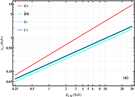
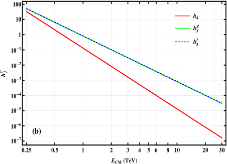
Figure 1: Unitarity bounds on new physics cutoff scales for the nTGC operators $(\mathcal{O}_{G+},\mathcal{O}_{\widetilde{B}W},\mathcal{O}_{G-},$ $\mathcal{O}_{C+})$ in plot (a) and for the nTGC form factors $(|h_{4}|,|h_{3}^{Z}|,|h_{3}^{\gamma}|)$ in plot (b). These bounds are derived from the $p$-wave amplitudes of the reaction $\hskip 0.85358ptf\bar{f}\!\rightarrow\!Z\gamma\hskip 0.85358pt$, where $\hskip 0.85358ptf\bar{f}\!=\!q\bar{q},e^{+}e^{-}$ with $q$ being the light quarks. 

In the cases of the nTGC form factors $(h_{4},\hskip 0.85358pth_{3}^{Z},\hskip 0.85358pth_{3}^{\gamma})$ defined in Eq.(3.5) of Section 3, they are connected to the cutoff scales of $(\mathcal{O}_{G+},\hskip 0.85358pt\mathcal{O}_{\widetilde{B}W},\hskip 0.85358pt\mathcal{O}_{G-})$ via $\,(|h_{4}|,|h_{3}^{Z},|h_{3}^{\gamma}|)\!=(r_{4}/\Lambda_{G+}^{4},r_{3}^{Z}/\Lambda_{\widetilde{B}W}^{4},r_{3}^{\gamma}/\Lambda_{G-}^{4})\hskip 0.85358pt$, as given by Eq.(3.6). Thus, using Eq.(2.24) we further derive the following unitarity bounds on the nTGC form factors:

$$|h_{4}|\! < \!\frac{\leavevmode\nobreak\ 24\sqrt{2\,}\pi v^{2}M_{Z}^{2}\leavevmode\nobreak\ }{s_{W}c_{W}s^{2}}\simeq\left(\!\frac{\,0.597\,\mathrm{TeV}\,}{\sqrt{s\,}}\!\right)^{\!\!4},$$ (2.25a)

$$|h_{3}^{V}|\! < \!\frac{\,6\sqrt{2\hskip 0.85358pt}\pi\hskip 0.85358pt\bar{r}_{3}^{V}\,}{\,s_{W}c_{W}C_{L,R}^{\prime}\,}\frac{\,v^{2}M_{Z}\,}{\sqrt{s^{3}\,}}\simeq\frac{\,0.350\hskip 0.85358pt\bar{r}_{3}^{V}\,}{\,C_{L,R}^{\prime}\hskip 0.85358pt}\!\left(\!\frac{\,\mathrm{TeV}\,}{\!\sqrt{s\,}\,}\!\right)^{\!\!3}\!,$$ (2.25b)

where we have used the expressions in Eq.(3.7b) for the coefficients $\,(r_{4},\hskip 0.85358ptr_{3}^{V})$ and have defined $\,\bar{r}_{3}^{V}\!\in\!(\bar{r}_{3}^{Z},\hskip 0.85358pt\bar{r}_{3}^{\gamma})\!=\!(1,\hskip 0.85358pts_{W}/c_{W})$.

Using formulae (2.24) and (2.25) for the unitarity bounds, we present their values in Table 1 for various sample values of the c.m. energies $\,E_{\mathrm{CM}}\!=\!(0.25,0.5,1,3,5,25)$TeV, of the reactions $\,q\bar{q}\!\rightarrow\!Z\gamma\,$ and $\,e^{-}e^{+}\!\!\rightarrow\!Z\gamma\,$ that are relevant to the present collider study. Then, in Fig. 1 we present the unitarity bounds on the nTGC operators and nTGC form factors as functions of the center-of-mass energy $\,E_{\mathrm{CM}}\!=\!(0.25-30)\hskip 0.85358pt$TeV for the reaction $\hskip 0.85358ptf\bar{f}\!\rightarrow\!Z\gamma\hskip 0.85358pt$, where $\hskip 0.85358ptf\bar{f}\!=\!q\bar{q},e^{+}e^{-}$ and $q$ denotes the light quarks. We plot the unitarity bounds on the new physics cutoff scales of the nTGC operators $(\mathcal{O}_{G+},\mathcal{O}_{\widetilde{B}W},\mathcal{O}_{G-},\mathcal{O}_{C+})$ in plot (a), whereas in plot (b) we impose the unitarity bounds on the nTGC form factors $(|h_{4}|,|h_{3}^{Z}|,|h_{3}^{\gamma}|)$, as derived from the $p$-wave amplitudes. Finally, by comparing the unitarity bounds of Table 1 and Fig. 1 with our collider bounds summarized in Tables 9-10 and in Figs. 10-11 of Section 5, we find that these perturbative unitarity bounds are much weaker than our collider bounds. Hence, they do not affect our collider analyses in the following Sections 4-5.

3 Form Factor Formulation for nTGCs

We study in this Section the form factor formulation of the neutral triple gauge vertices (nTGVs) $Z\gamma V^{*}$. After imposing Lorentz invariance, the residual electromagnetic $U(1)_{\mathrm{em}}$ gauge symmetry and CP conservation, they are conventionally expressed in the following form [3][4]:

$$\Gamma_{Z\gamma V^{*}}^{\alpha\beta\mu}(q_{1},q_{2},q_{3})\!\! = \!\!\frac{\leavevmode\nobreak\ e\hskip 0.85358pt(q_{3}^{2}-M_{V}^{2})\,}{\,M_{Z}^{2}\leavevmode\nobreak\ }\!\left(\!h_{3}^{V}\hskip 0.85358ptq_{2\nu}\epsilon^{\alpha\beta\mu\nu}\!+\frac{h_{4}^{V}}{\,M_{Z}^{2}\,}\hskip 0.85358ptq_{2}^{\alpha}\hskip 0.85358ptq_{3\nu}\hskip 0.85358ptq_{2\sigma}\epsilon^{\beta\mu\nu\sigma}\!\right)\!,\hskip 45.5244pt$$ (3.1)

where the gauge bosons are denoted by $\,V\!\!\equiv\!Z,\gamma$ and the form factor parameters $(h_{3}^{V},\,h_{4}^{V})$ are treated as constant coefficients for the purposes of experimental tests [18].

We stress that the spontaneous breaking of the SM electroweak gauge symmetry requires the nTGCs to be generated only by the gauge-invariant effective operators of dimension-8 or higher. This implies that the consistent form factor formulation of the neutral triple gauge vertices must map precisely the expressions for these gauge-invariant nTGC operators in the broken phase. This precise mapping between the nTGVs in the broken phase of these dimension-8 nTGC operators (2.2) imposes nontrivial relations between the parameters of the nTGVs in the form factor formulation and removes possible unphysical energy-dependent terms in them.

By direct power counting, we find that the dimension-8 operator $\mathcal{O}_{G+}$ contributes to the nTGVs with a leading $\hskip 0.85358ptE^{5}\hskip 0.85358pt$ energy dependence. Based on this and the above observations, we find that the conventional form factor formula (3.1) is not compatible with the gauge-invariant SMEFT formulation, and a new term must be added, labelled by $h_{5}^{V}$ in the following. With these remarks in mind, we express the neutral triple gauge vertices $Z\gamma V^{*}$ as follows:

$$\Gamma_{Z\gamma V^{*}}^{\alpha\beta\mu(8)}(q_{1},q_{2},q_{3})\,=\,\frac{\,e\hskip 0.85358pt(q_{3}^{2}-\!M_{V}^{2})\,}{\,M_{Z}^{2}\,}\!\left[\!\left(h_{3}^{V}\!+h_{5}^{V}\frac{q_{3}^{2}}{\,M_{Z}^{2}\,}\right)\!q_{2\nu}\epsilon^{\alpha\beta\mu\nu}+\displaystyle\frac{h_{4}^{V}}{\,M_{Z}^{2}\,}\hskip 0.85358ptq_{2}^{\alpha}\hskip 0.85358ptq_{3\nu}\hskip 0.85358ptq_{2\sigma}\hskip 0.85358pt\epsilon^{\beta\mu\nu\sigma}\right]\!,$$ (3.2)

where the form factors $h_{i}^{V}$ are taken as constants in the present study. The parametrization of the nTGVs in Eq.(3.2) corresponds to the following effective Lagrangian:

$$\mathcal{L}\,=\, \frac{e}{\,M_{Z}^{2}\,}\!\Bigg{[}\!-\!\left[h_{3}^{\gamma}(\partial_{\sigma}F^{\sigma\rho})+h_{3}^{Z}(\partial_{\sigma}Z^{\sigma\rho})+\!\frac{h_{5}^{\gamma}}{\,M_{Z}^{2}\,}(\partial^{2}\partial_{\sigma}F^{\rho\sigma})+\frac{h_{5}^{Z}}{\,M_{Z}^{2}\,}(\partial^{2}\partial_{\sigma}Z^{\rho\sigma})\right]\!Z^{\alpha}\widetilde{F}_{\rho\alpha}$$

$$\hskip 28.45274pt+\left\{\!\frac{h_{4}^{\gamma}}{\,2M_{Z}^{2}\,}\!\left[\square\partial^{\sigma}\!F^{\rho\alpha}\right]+\frac{h_{4}^{Z}}{\,2M_{Z}^{2}\,}\!\left[(\square+\!M_{Z}^{2})\partial^{\sigma}\!Z^{\rho\alpha}\right]\!\right\}\!Z_{\sigma}\widetilde{F}_{\rho\alpha}\Bigg{]}.$$ (3.3)

which differs from the conventional nTGV form factor Lagrangian [2] by the new $h_{5}^{V}$ terms.

We now compare our modified nTGV formula (3.2) with the nTGVs in Eqs.(2.4a)-(2.4d) as predicted by the gauge-invariant dimension-8 nTGC operators $(\mathcal{O}_{G+},\,\mathcal{O}_{G-},\,\mathcal{O}_{\widetilde{B}W})$ in Eqs.(2.2a)-(2.2c), which should match exactly case by case. In the case of the operator $\mathcal{O}_{G+}$, this matching leads to the following two restrictions on the form factors in Eq.(3.2):

$$h_{4}^{V} \,=\,2\hskip 0.85358pth_{5}^{V}\,,$$ (3.4a)

$$h_{4}^{Z}\hskip 0.85358pt =\hskip 0.85358pt\frac{\,c_{W}\,}{s_{W}}\hskip 0.85358pth_{4}^{\gamma}\,,$$ (3.4b)

where henceforward we denote $\hskip 0.85358pth_{4}\equiv h_{4}^{Z}\hskip 1.42262pt$ for convenience. These conditions demonstrates that there are only three independent form-factor parameters $(h_{3}^{Z},\hskip 0.85358pth_{3}^{\gamma},\hskip 0.85358pth_{4})$. Applying the condition (3.4a), we can express the $Z\gamma V^{*}$ vertex (3.2) as follows:

$$\Gamma_{Z\gamma V^{*}}^{\alpha\beta\mu(8)}(q_{1},q_{2},q_{3})\,=\,\frac{\,e\hskip 0.85358pt(q_{3}^{2}-\!M_{V}^{2})\,}{\,M_{Z}^{2}\,}\!\left[\!\left(\!h_{3}^{V}\!+\!\frac{\,h_{4}^{V}\,}{\,2M_{Z}^{2}\,}q_{3}^{2}\right)\!q_{2\nu}\hskip 0.85358pt\epsilon^{\alpha\beta\mu\nu}+\frac{h_{4}^{V}}{\,M_{Z}^{2}\,}\hskip 0.85358ptq_{2}^{\alpha}\hskip 0.85358ptq_{3\nu}\hskip 0.85358ptq_{2\sigma}\hskip 0.85358pt\epsilon^{\beta\mu\nu\sigma}\right]\!.$$ (3.5)

Comparing the nTGVs (2.4) predicted by the dimension-8 operators (2.2a)-(2.2c) with the form factor formulation (3.5) of the nTGVs, we can connect the three independent form-factor parameters $(h_{3}^{Z},\hskip 0.85358pth_{3}^{\gamma},\hskip 0.85358pth_{4})$ to the cutoff scales $(\Lambda_{G+},\hskip 0.85358pt\Lambda_{G-},\hskip 0.85358pt\Lambda_{\widetilde{B}W})$ of the corresponding dimension-8 operators $(\mathcal{O}_{G+},\hskip 0.85358pt\mathcal{O}_{G-},\hskip 0.85358pt\mathcal{O}_{\widetilde{B}W})$, as follows:

$$h_{4} =-\frac{\leavevmode\nobreak\ \text{sign}(\tilde{c}_{G+})\,}{\,\Lambda^{4}_{G+}\,}\frac{v^{2}M_{Z}^{2}}{\,s_{W}c_{W}\,}\equiv\!\frac{r_{4}}{\,[\Lambda^{4}_{G+}]\,}\hskip 0.85358pt, h_{3}^{V}\!=0\hskip 0.85358pt, \hskip 0.85358pt\text{for}\leavevmode\nobreak\ \mathcal{O}_{G+}\hskip 0.85358pt\hskip 0.85358pt,\hskip 14.22636pt$$ (3.6a)

$$h_{3}^{Z} =\frac{\,\text{sign}(\tilde{c}_{\!\widetilde{B}W})\,}{\,\Lambda_{\!\widetilde{B}W}^{4}\,}\frac{v^{2}M_{Z}^{2}}{\leavevmode\nobreak\ 2s_{W}c_{W}\,}\equiv\!\frac{r_{3}^{Z}}{\,[\Lambda^{4}_{\widetilde{B}W}]\,}\hskip 0.85358pt, h_{3}^{\gamma},h_{4}^{V}\!=0\hskip 0.85358pt, \hskip 0.85358pt\text{for}\leavevmode\nobreak\ \mathcal{O}_{\widetilde{B}W}\hskip 0.85358pt\hskip 0.85358pt,$$ (3.6b)

$$h_{3}^{\gamma} =-\frac{\,\text{sign}(\tilde{c}_{G-})\,}{\,\Lambda_{G-}^{4}\,}\frac{v^{2}M_{Z}^{2}}{\leavevmode\nobreak\ 2c_{W}^{2}\,}\equiv\!\frac{r_{3}^{\gamma}}{\,[\Lambda^{4}_{G-}]\,}\,. h_{3}^{Z},h_{4}^{V}\!=0\hskip 0.85358pt, \hskip 0.85358pt\text{for}\leavevmode\nobreak\ \mathcal{O}_{G-}\hskip 0.85358pt\hskip 0.85358pt,$$ (3.6c)

where the form factor $h_{4}$ is defined below Eq.(3.4) and we have used the notations:

$$[\Lambda^{4}_{G+}]=\text{sign}(\tilde{c}_{G+})\Lambda^{4}_{G+}\hskip 0.85358pt,\leavevmode\nobreak\ \leavevmode\nobreak\ \leavevmode\nobreak\ [\Lambda^{4}_{\widetilde{B}W}]=\text{sign}(\tilde{c}_{\!\widetilde{B}W})\Lambda^{4}_{\widetilde{B}W}\hskip 0.85358pt,\leavevmode\nobreak\ \leavevmode\nobreak\ \leavevmode\nobreak\ [\Lambda^{4}_{G-}]=\text{sign}(\tilde{c}_{G-})\Lambda^{4}_{G-}\hskip 0.85358pt,$$ (3.7a)

$$r_{4}=-\frac{\leavevmode\nobreak\ v^{2}M_{Z}^{2}\leavevmode\nobreak\ }{\,s_{W}c_{W}\,}\hskip 0.85358pt,\leavevmode\nobreak\ \leavevmode\nobreak\ \leavevmode\nobreak\ \leavevmode\nobreak\ \leavevmode\nobreak\ r_{3}^{Z}=\frac{v^{2}M_{Z}^{2}}{\leavevmode\nobreak\ 2s_{W}c_{W}\,}\hskip 0.85358pt,\leavevmode\nobreak\ \leavevmode\nobreak\ \leavevmode\nobreak\ \leavevmode\nobreak\ \leavevmode\nobreak\ r_{3}^{\gamma}=-\frac{\leavevmode\nobreak\ v^{2}M_{Z}^{2}\leavevmode\nobreak\ }{\leavevmode\nobreak\ 2c_{W}^{2}\,}\hskip 0.85358pt.$$ (3.7b)

From the above, we see that only the operator $\mathcal{O}_{G+}$ can directly contribute to the form factor $h_{4}^{V}$, as in Eq.(3.6a), which can be understood from the explicit formulae (2.4a). We note that the operator $\hskip 0.85358pt\mathcal{O}_{\widetilde{B}W}$ contains Higgs-doublet fields and thus cannot contribute to the $\hskip 0.85358pth_{4}^{V}$ term in Eq.(3.5), but $\hskip 0.85358pt\mathcal{O}_{\widetilde{B}W}\!$ can contribute to the $\hskip 0.85358pth_{3}^{Z}$ term through the $Z\gamma Z^{*}$ vertex and leaves $\hskip 0.85358pth_{3}^{\gamma}\!=0\hskip 0.85358pt$, as shown in Eq.(3.6b). The operator $\mathcal{O}_{G-}$ also cannot contribute to $h_{4}^{V}$ due to the equation of motion (2.3a), $\mathcal{O}_{G-}\!\!=\mathcal{O}_{\widetilde{B}W}\!+\mathcal{O}_{C+}$, where $\mathcal{O}_{C+}$ contains a bilinear fermion factor and cannot contribute directly to the nTGC. The fact that $\mathcal{O}_{G-}$ is irrelevant to $h_{4}^{V}$ is also shown explicitly in Eq.(2.4d).  The explicit formula (2.4d) further shows that $\mathcal{O}_{G-}$ makes a nonzero contribution to $h_{3}^{\gamma}\hskip 0.85358pt$, but leaves $\hskip 0.85358pth_{3}^{Z}\!=0\hskip 0.85358pt$, as we find in Eq.(3.6c) above.

Using Eq.(3.2) or (3.5) and by direct power counting, we infer the following leading energy-dependences of the $h_{i}^{V}$ contributions to the helicity amplitudes $\hskip 0.85358pt\mathcal{T}[f\bar{f}\!\rightarrow\!Z\gamma]\,$:

$$\mathcal{T}_{(8)}^{ss^{\prime}\!,\text{T}} = \!\!h_{3}^{V}O(E^{2})+h_{5}^{V}O(E^{4})\,,$$ (3.8a)

$$\mathcal{T}_{(8)}^{ss^{\prime}\!,\text{L}} = \!\!h_{3}^{V}O(E^{3})+h_{4}^{V}O(E^{5})+h_{5}^{V}O(E^{5})\,.\hskip 51.21495pt$$ (3.8b)

We note in Eq.(3.8a) that the form factor $\,h_{4}^{V}\hskip 0.85358pt$ does not contribute to the production of a transversely polarized $Z$ boson in the final state, because the $s$-channel momentum $\,q_{3}^{\alpha}\,$ has no spatial component and the $Z$ boson’s transverse polarization vector $\hskip 0.85358pt\epsilon_{T\alpha}\hskip 0.85358pt$ has no time component, and thus $\,q_{3}^{\alpha}\epsilon_{T\alpha}^{*}\!=0\hskip 0.85358pt$.

Inspecting Eq.(3.8), it would appear that the leading energy-dependence of $\,\mathcal{T}_{(8)}^{ss^{\prime}\!,\text{L}}$ should be $\mathcal{O}(E^{5})$. However, we observe that the helicity amplitudes including a final-state longitudinal $Z$ boson as contributed by the gauge-invariant dimension-8 nTGC operators must obey the equivalence theorem (ET) [22]. At high energies $E\!\gg\!M_{Z}\hskip 0.85358pt$, the ET takes the following form:

$$\vspace*{-2mm}\mathcal{T}_{(8)}[Z_{L},\gamma_{T}]\,=\,\mathcal{T}_{(8)}[-\mathrm{i}\pi^{0},\gamma_{T}]+B\,,$$ (3.9)

where the longitudinal gauge boson $Z_{L}$ absorbs the would-be Goldstone boson $\pi^{0}$ through the Higgs mechanism, and the residual term $\,B=\mathcal{T}_{(8)}[v^{\mu}Z_{\mu},\gamma_{T}]\,$ is suppressed by the relation $\,v^{\mu}\!\hskip 0.85358pt\equiv\!\epsilon_{L}^{\mu}-$ $q_{Z}^{\mu}/M_{Z}=O(M_{Z}/E_{Z})$ [22]. However, we cannot apply the ET (3.9) directly to the form factor formulation (3.2), because it does not respect the full electroweak gauge symmetry of the SM and contains no would-be Goldstone boson. We stress again that the electroweak gauge-invariant formulation of the nTGCs can be derived only from the dimension-8 operators as in Eq.(2.2). Hence, we study the allowed leading energy-dependences of the helicity amplitudes (3.8) by applying the ET to the contributions of the dimension-8 nTGC operators (2.2). Then, we find that only the operator $\mathcal{O}_{\widetilde{B}W}$ could give a nonzero contribution to the Goldstone amplitude $\,\mathcal{T}_{(8)}[-\mathrm{i}\pi^{0},\gamma_{T}]\,$, with a leading energy-dependence $\mathcal{O}(E^{3})$ that corresponds to the form factor $h_{3}^{Z}\hskip 0.85358pt$. The operator $\hskip 0.85358pt\mathcal{O}_{G_{+}}\!$ does not contribute to the Goldstone amplitude $\mathcal{T}_{(8)}[-\mathrm{i}\pi^{0},\gamma_{T}]$, but can contribute the largest residual term $B=\mathcal{O}(E^{3})$. From these facts, we deduce that in Eq.(3.8b) the $\mathcal{O}(E^{5})$ terms due to the form factors $h_{4}^{V}$ and $h_{5}^{V}$ must exactly cancel each other, from which we derive the following condition,

$$h_{4}^{V}/\hskip 0.85358pth_{5}^{V}\,=\,2\,,$$ (3.10)

which agrees with Eq.(3.4a). Then, using our improved form factor formulation (3.5) of the nTGCs, we can compute the corresponding helicity amplitudes of $\hskip 0.85358ptf\bar{f}\!\rightarrow\!Z\gamma\hskip 0.85358pt$ from the nTGC contributions:

$$\mathcal{T}_{(8),\text{F}}^{ss^{\prime}\!,\text{T}}\!\!\left\lgroup\!\!\!\begin{array}[]{cc}--\!&\!-+\\ +-\!&\!++\\ \end{array}\!\!\!\right\rgroup\!\!=\frac{\,(c_{L}^{V}\!\!+\!c_{R}^{V})e^{2}(2h^{V}_{3}M_{Z}^{2}+h_{4}^{V}s)(s\!-\!M_{Z}^{2})\sin\!\theta\,}{4M_{Z}^{4}c_{W}s_{W}}\!\!\left\lgroup\!\!\begin{array}[]{cr}1\nobreak\leavevmode&0\\[2.84526pt] 0\nobreak\leavevmode&-1\end{array}\!\!\right\rgroup\!\!,$$ (3.11e)

$$\mathcal{T}_{(8),\text{F}}^{ss^{\prime}\!,\text{L}}(0-,0+)=\frac{\,\sqrt{2\,}\hskip 0.85358pte^{2}(s\!-\!M_{Z}^{2})\sqrt{s\,}\,}{4M_{Z}^{3}c_{W}s_{W}}(2h_{3}^{V}\!+h_{4}^{V})\!\left(\!c_{L}^{V}\!\sin^{2}\!\frac{\theta}{2}\!-c_{R}^{V}\cos^{2}\!\frac{\theta}{2},\leavevmode\nobreak\ c_{R}^{V}\sin^{2}\!\frac{\theta}{2}\!-c_{L}^{V}\cos^{2}\!\frac{\theta}{2}\right)\!,$$ (3.11f)

where the coupling coefficients are defined as $\,(c_{L}^{Z},\hskip 0.85358ptc_{R}^{Z})\!=(T_{3}-Qs_{W}^{2},-Qs_{W}^{2})$ for $V\!\!=Z\hskip 0.85358pt$ and $\,c_{L}^{A}=c_{R}^{A}=Qc_{W}s_{W}$ for $V\!=\gamma\hskip 0.85358pt$. On the right-hand-side of the above formulas, the subscript “ F ” indicates contributions given by the form factors. From the above, we see that the helicity amplitude $\hskip 0.85358pt\mathcal{T}_{(8)}^{ss^{\prime}\!,\text{T}}$ for the transverse $Z_{T}$ final state contains the $O(E^{2})$ contribution from the form factor $\hskip 0.85358pth_{3}^{V}$ and the leading contribution of $O(E^{4})$ from the form factor $\hskip 0.85358pth_{4}^{V}$, while the the helicity amplitude $\hskip 0.85358pt\mathcal{T}_{(8)}^{ss^{\prime}\!,\text{L}}$ for the longitudinal $Z_{L}$ final state has a leading contribution of $O(E^{3})$ from the form factor combination $\hskip 0.85358pt(2h_{3}^{V}\!+h_{4}^{V})\hskip 0.85358pt$.

We note that the operators $\mathcal{O}_{C+}$ and $\mathcal{O}_{C-}$ both contain only left-handed fermions, and recall that the operators $\mathcal{O}_{G+}$ and $\mathcal{O}_{C-}$ give the same contributions to the amplitude $\mathcal{T}[f\bar{f}\!\rightarrow\!Z\gamma]\hskip 0.85358pt$, due to the equation of motion (2.3b). Thus, we find that the ratio $\hskip 0.85358pth_{4}^{Z}/h_{4}^{\gamma}\hskip 0.85358pt$ must be fixed to cancel their contributions to the amplitude $\,\mathcal{T}[f\bar{f}\!\!\rightarrow\!Z^{*}\!\!\rightarrow\!\!Z\gamma]+\mathcal{T}[f\bar{f}\!\!\rightarrow\!\gamma^{*}\!\!\rightarrow\!\!Z\gamma]$ via right-handed fermions [5]. This imposes the following condition on the two form factors $(h_{4}^{Z},\hskip 0.85358pth_{4}^{\gamma})$:

$$h_{4}\,\equiv\,h_{4}^{Z}\hskip 0.85358pt=\hskip 0.85358pt\frac{\,c_{W}\,}{s_{W}}\hskip 0.85358pth_{4}^{\gamma}\hskip 0.85358pt,$$ (3.12)

for the $\mathcal{O}_{G+}$ operator. This condition agrees with Eq.(3.4b), which we derived earlier by matching the prediction of the operator $\mathcal{O}_{G+}$ with the nTGV formulation (3.2). Hence, using the gauge-invariant dimension-8 nTGC operators to derive the form factor formulation (3.2), we deduce that there are only three independent form-factor parameters $(h_{3}^{Z},\hskip 0.85358pth_{3}^{\gamma},\hskip 0.85358pth_{4})$, where $\hskip 0.85358pth_{4}\equiv h_{4}^{Z}$ and $\hskip 0.85358pth_{4}^{\gamma}\hskip 0.85358pt$ are connected by the condition (3.12).

The fermionic dimension-8 operators $\mathcal{O}_{C+}$ and $\mathcal{O}_{C-}$ contribute to the quartic vertex $f\bar{f}Z\gamma\hskip 0.85358pt$, but do not contribute directly to the nTGC vertex $Z\gamma V^{*}$ in Eq.(3.5). We can factorize their contribution to the on-shell quartic vertex $f\bar{f}Z\gamma\hskip 0.85358pt$ as follows:

$$\Gamma^{\alpha\beta}_{\!f\bar{f}Z\gamma}(q_{1},q_{2})\,=\,\sum_{V}\Gamma_{\mu}(f\bar{f}V^{*})P_{L}\times(q_{3}^{2}-\!M_{V}^{2})^{-1}\!\times\Gamma_{Z\gamma V^{*}}^{\alpha\beta\mu}(q_{1},q_{2},q_{3})\,,$$ (3.13)

which includes effectively an nTGC vertex $\hskip 0.85358pt\Gamma_{Z\gamma V^{*}}^{\alpha\beta\mu}\hskip 0.85358pt$. This effective nTGC vertex function $\hskip 0.85358pt\Gamma_{Z\gamma V^{*}}^{\alpha\beta\mu}\hskip 0.85358pt$ contains the form factor parameters $(h_{3}^{Z},\hskip 0.85358pth_{3}^{\gamma})$ for the operator $\mathcal{O}_{C+}\hskip 0.85358pt$.  Since $\mathcal{O}_{C+}$ involves purely left-handed fermions, we find that the ratio $\hskip 0.85358pth_{3}^{Z}/h_{3}^{\gamma}\hskip 0.85358pt$ must be fixed, so as to cancel its contributions to the amplitude $\,\mathcal{T}[f\bar{f}\!\!\rightarrow\!Z^{*}\!\!\rightarrow\!\!Z\gamma]+\mathcal{T}[f\bar{f}\!\!\rightarrow\!\gamma^{*}\!\!\rightarrow\!\!Z\gamma]$ via right-handed fermions. This imposes the following condition between form factors $(h_{3}^{Z},\hskip 0.85358pth_{3}^{\gamma})$:

$$h_{3}\,\equiv\,h_{3}^{Z}\hskip 0.85358pt=\hskip 0.85358pt\frac{\,c_{W}\,}{s_{W}}\hskip 0.85358pth_{3}^{\gamma}\hskip 0.85358pt,\hskip 34.1433pt\hskip 0.85358pt\text{for}\leavevmode\nobreak\ \mathcal{O}_{C+}\hskip 0.85358pt\hskip 0.85358pt.$$ (3.14)

We note that the above relation holds only for the fermionic operator $\hskip 0.85358pt\mathcal{O}_{C+}\hskip 0.85358pt$. For the other fermionic operator $\mathcal{O}_{C-}$, its contribution to the effective nTGC vertex function $\hskip 0.85358pt\Gamma_{Z\gamma V^{*}}^{\alpha\beta\mu}\hskip 0.85358pt$ in Eq.(3.13) contains the same form factors $(h_{4}^{Z},\hskip 0.85358pth_{4}^{\gamma})$ as that of the operator $\mathcal{O}_{G+}$, because the equation of motion guarantees [5] that both of the operators $\mathcal{O}_{G+}$ and $\mathcal{O}_{C-}$ give the same contributions to the on-shell quartic vertex $f\bar{f}Z\gamma\hskip 0.85358pt$. Thus, the form factors $(h_{4}^{Z},\hskip 0.85358pth_{4}^{\gamma})$ of the effective nTGC vertex function $\hskip 0.85358pt\Gamma_{Z\gamma V^{*}}^{\alpha\beta\mu}\hskip 0.85358pt$ of the left-handed fermionic operator $\mathcal{O}_{C-}$ obey the same cancellation condition Eq.(3.4b).

4 Probing nTGCs at the LHC and Future $pp$ Colliders

In this Section we will analyze the sensitivity reaches on probing the nTGCs at the LHC and future $p{\hskip 0.85358pt}p$ colliders via the reactions $\hskip 0.85358ptp{\hskip 0.85358pt}p{\hskip 0.85358pt}(q{\hskip 0.85358pt}\bar{q})\!\rightarrow\!Z\gamma\hskip 0.85358pt$ with $Z\!\rightarrow\!\ell^{+}\ell^{-}\!,\hskip 0.85358pt\nu{\hskip 0.85358pt}\bar{\nu}{\hskip 0.85358pt}\hskip 0.85358pt$. In Section 4.1, we give the setup for the analyses. In Sections 4.2-4.3, we present the analyses of nTGCs at ${\cal O}(\Lambda^{\!-4})$ and ${\cal O}(\Lambda^{\!-8})$ respectively. In the analysis of Section 4.4, we further include the decay channel of $Z\!\rightarrow\!\nu{\hskip 0.85358pt}\bar{\nu}$. Then, we study the probes of the nTGV form factor in Section 4.5, and the correlations between the nTGC sensitivities in Section 4.6. Finally, we compare in Section 4.7 our predicted LHC sensitivity reaches on the nTGCs with the published LHC experimental limits by both the ATLAS and CMS collaborations.

4.1 Setup for the Analyses at Hadron Colliders

The distributions of quark and antiquark momenta in protons are given by parton distribution functions (PDFs). At leading order, the total cross section of $\,p{\hskip 0.85358pt}p\!\rightarrow\!Z\gamma\hskip 0.85358pt$ at the LHC is calculated by integrating the convolved product of the quark and antiquark PDFs and the parton-level cross section of the $\hskip 0.85358ptq\hskip 0.85358pt\bar{q}\!\rightarrow\!Z\gamma\hskip 0.85358pt$ subprocess:

$$\sigma\leavevmode\nobreak\ =\leavevmode\nobreak\ \sum_{q,\bar{q}\,}\!\int\!\!\text{d}x_{1}\hskip 0.85358pt\text{d}x_{2}\left[\mathcal{F}_{\!q/p}(x_{1},\mu)\hskip 0.85358pt\mathcal{F}_{\!\bar{q}/p}(x_{2},\mu)\hskip 1.42262pt{\sigma}_{\!q\bar{q}}(\hat{s})+(q\leftrightarrow\bar{q})\right]\!,$$ (4.1)

where the functions $\mathcal{F}_{\!q/p}$ and $\mathcal{F}_{\!\bar{q}/p}$ are the PDFs of the quark and antiquark in the proton beams, and $\,\hat{s}\!=\!x_{1}\hskip 0.85358ptx_{2}\hskip 0.85358pts\,$ with the collider energy $\sqrt{s\,}\!=\!13\,\text{TeV}\hskip 0.85358pt$. The PDFs depend on the factorization scale $\mu$, which is set to be $\,\mu\!=\!\sqrt{\hat{s}\,}/2\,$ in our leading-order analysis. We use the PDFs of the quarks $\hskip 0.85358ptq=u,d,s,c,b\hskip 0.85358pt$ and their antiquarks determined by the CTEQ collaboration [23].

During LHC Run-2 the ATLAS measurements of the $\ell^{+}\ell^{-}\gamma$ and $\bar{\nu}\nu\gamma$ final states reached a maximum value of $M_{\ell\ell\gamma}\!\sim\!3$ TeV. Accordingly, we set $\hat{s}\lesssim 3$ TeV for our LHC analysis and use an upper limit $\hat{s}\lesssim 23$ TeV for the 100 TeV $pp$ collider.

We compute the production cross section of $\hskip 0.85358ptq\hskip 0.85358pt\bar{q}\!\rightarrow\!Z\gamma\hskip 0.85358pt$ at leading order (LO) in QCD and ${\cal O}(\alpha^{2})$ for the SM, and $O(\alpha^{1.5}\tilde{c}_{j})$ or $O(\alpha\tilde{c}_{j}^{2})$ for the nTGCs, where $\alpha\!=\!\alpha_{\mathrm{em}}$ or $\alpha_{\mathrm{w}}$, as the possible high-order contributions are not important for our study. There are next-to-leading-order (NLO) QCD corrections from the gluon-induced loop diagrams for $\hskip 0.85358ptq\hskip 0.85358pt\bar{q}\rightarrow Z\gamma\hskip 0.85358pt$ and the real emission of a gluon: $\hskip 0.85358ptq\hskip 0.85358pt\bar{q}\!\rightarrow\!Z\gamma+g\hskip 0.85358pt$, and there are also NLO QCD contributions from $g\hskip 0.85358ptq\!\rightarrow\!Z\gamma+q$ $(\hskip 0.85358ptg\hskip 0.85358pt\bar{q}\!\rightarrow\!Z\gamma+\bar{q}\hskip 0.85358pt)\hskip 0.85358pt$. In these cases the NLO/LO ratio is ${\cal O}(\alpha_{s})$, and it was found numerically that the effect of adding the full NNLO corrections is less than 10% [24][25][26]. We define a QCD $K$-factor for the nTGC signal by $\hskip 0.85358ptK_{\mathrm{S}}\!\equiv\!S\hskip 0.85358pt/S_{\mathrm{LO}}\!=\!1\!+\!\Delta K_{\mathrm{S}}\hskip 0.85358pt$ and for the SM background by $\hskip 0.85358ptK_{\mathrm{B}}\!\equiv\!B/B_{\mathrm{LO}}\!=\!1\!+\!\Delta K_{B}\hskip 0.85358pt$. We have checked the $K$-factors for $\hskip 0.85358ptpp\!\rightarrow\!Z\gamma\hskip 0.85358pt$ by using Madgraph5@NLO [27], and find that they depend on the kinematic cuts. The corrections $\Delta K$ can be larger than one if only basic cuts are made, but we find that adding a cut to remove the small $P_{T}(\gamma)$ region and vetoing extra jets in the final state reduces $\Delta K\hskip 0.85358pt$ to only a few percent, which may be neglected.

We note in addition that $Z\gamma$ production by the gluon fusion process is formally a next-to-next-to-leading-order (NNLO) contribution, and is found to be generally less than 1% [28]. The nTGC contributions via gluon fusion is also found to be negligible [28].

Next, we discuss the statistical significance and its optimization for our present analysis of sensitivity reaches on the nTGCs. Since the SM contribution $\sigma_{0}$ could be small, the ratio $\hskip 0.85358ptS/\sqrt{B\,}\hskip 0.85358pt$ is not an optimal measure of the statistical significance. We use instead the following formula for the background-with-signal hypothesis [32]:

$$\mathcal{Z}\,=\,\sqrt{2\!\left(\!B\ln\!\frac{\,B\,}{\,B+S\,}+S\right)\,}\,=\,\sqrt{2\!\left(\!\sigma_{0}\ln\!\frac{\,\sigma_{0}\,}{\,\sigma_{0}+\Delta\sigma\,}+\Delta\sigma\!\right)\,}\times\sqrt{\mathcal{L}\times\epsilon\leavevmode\nobreak\ },$$ (4.2)

where $\hskip 0.85358pt\Delta\sigma=\sigma-\sigma_{0}\hskip 0.85358pt$ denotes the part of the cross section beyond the SM contribution, $\hskip 0.85358pt\mathcal{L}\hskip 0.85358pt$ is the integrated luminosity, and $\hskip 0.85358pt\epsilon\hskip 0.85358pt$ is the detection efficiency. When $\hskip 0.85358ptB\!\gg\!S\hskip 0.85358pt$, we can expand (4.12) in terms of $\,S/B\,$ and find that it reduces to the form $\,\mathcal{Z}\!\simeq\!S/\!\sqrt{B\,}$, whereas for $\hskip 0.85358ptS\!\gg\!B\hskip 0.85358pt$ it reduces to $\,\mathcal{Z}\!\simeq\!\sqrt{2S\,}\hskip 0.85358pt$. If the signal $S$ is dominated by the interference contribution of $O(\Lambda^{-4})$, we can deduce that the sensitivity reach on the new physics scale:

$$\Lambda\propto(\mathcal{L}\times\epsilon)^{1/8},\,\hskip 39.83385pt(\text{for}\leavevmode\nobreak\ B\!\gg\!S\hskip 0.85358pt),$$ (4.3a)

$$\Lambda\propto(\mathcal{L}\times\epsilon)^{1/4},\,\hskip 39.83385pt(\text{for}\leavevmode\nobreak\ S\!\gg\!B\hskip 0.85358pt).$$ (4.3b)

If the signal $S$ is dominated by the squared contribution of $O(\Lambda^{-8})$, we can deduce that the sensitivity reach on the new physics scale:

$$\Lambda\propto(\mathcal{L}\times\epsilon)^{1/16},\,\hskip 39.83385pt(\text{for}\leavevmode\nobreak\ B\!\gg\!S\hskip 0.85358pt),$$ (4.4a)

$$\Lambda\propto(\mathcal{L}\times\epsilon)^{1/8},\,\hskip 44.10176pt(\text{for}\leavevmode\nobreak\ S\!\gg\!B\hskip 0.85358pt).$$ (4.4b)

In either case, we see that the bound on the new physics scale $\Lambda$ is not very sensitive to the integrated luminosity $\hskip 0.85358pt\mathcal{L}\hskip 0.85358pt$ and the detection efficiency $\hskip 0.85358pt\epsilon\hskip 0.85358pt$. For instance, in the case of $B\!\gg\!S$, if the integrated luminosity $\hskip 0.85358pt\mathcal{L}\,$ increases by a factor of $10\hskip 1.42262pt$, we find that the sensitivity reach of $\hskip 0.85358pt\Lambda\hskip 0.85358pt$ is enhanced by about 33% when the interference contribution dominates the signal and 15% when the squared contribution dominates the signal. If the detection efficiency $\hskip 0.85358pt\epsilon\hskip 0.85358pt$ is reduced from the ideal value of $\hskip 0.85358pt\epsilon\!=\!1\hskip 0.85358pt$ to $\hskip 0.85358pt\epsilon\!=\!0.5\hskip 0.85358pt$, we find that the sensitivity reach of $\Lambda$ is weakened by only about 8% when the interference contribution dominates the signal and 4% when the squared contribution dominates the signal.

In order to achieve higher sensitivity, we can discriminate between the signal and background by using the photon $P_{T}$ distribution, employing the following measure of significance:

$$\mathcal{Z}_{\mathrm{total}}\,=\,\sqrt{\,\sum\!\mathcal{Z}_{\mathrm{bin}}^{2}\leavevmode\nobreak\ }\,.$$ (4.5)

In the above, we impose the optimal cut on the photon $P_{T}$ for each bin and compute the corresponding significance $\mathcal{Z}_{\mathrm{bin}}$ of each bin. By doing so, we maximize the significance $\hskip 0.85358pt\mathcal{Z}_{\mathrm{total}}\hskip 0.85358pt$ given in Eq.(4.5).

4.2 Analysis of nTGCs at ${\cal O}(\Lambda^{\!-4})$

We compute analytically the parton-level cross section of the annihilation process $\hskip 0.85358ptq\hskip 0.85358pt\bar{q}\!\rightarrow\!Z\gamma\hskip 0.85358pt$, and then perform the convolved integration over the product of the quark and antiquark PDFs to obtain the cross section for $\hskip 0.85358ptp{\hskip 0.85358pt}p{\hskip 0.85358pt}(q{\hskip 0.85358pt}\bar{q})\!\rightarrow\!Z\gamma\hskip 0.85358pt$.

Inspecting the azimuthal angular distributions in Eq.(2.14), we note that the SM $\phi_{*}$ distribution $\hskip 0.85358ptf_{\phi_{*}}^{0}$ is nearly flat, whereas the maximum of the nTGC contribution $\hskip 0.85358ptf_{\phi_{*}}^{1}$ is at $\hskip 0.85358pt\phi_{*}=0\hskip 1.42262pt$. We consider the double differential cross section with respect to the photon transverse momentum $P_{T}$ and $\phi_{*}$ at $\hskip 0.85358pt\phi_{*}\!=0\hskip 0.85358pt$,

$$f_{{P_{T}}}^{j}\,=\,\left.\frac{2\pi\hskip 0.85358pt\text{d}^{2}\sigma_{j}}{\,\text{d}{P_{T}}\,\text{d}\phi_{*}\,}\right|_{\phi_{*}=\hskip 0.85358pt0}.$$ (4.6)

Eq.(2.14) gives $\,\text{d}\sigma_{0}/\text{d}\phi_{*}\simeq\sigma_{0}/(2\pi)\hskip 0.85358pt$ for the SM contribution, so we can deduce:

$$f_{P_{T}}^{0}\,\simeq\frac{\,\text{d}\sigma_{0}\,}{\,\text{d}P_{T}\,}\,.$$ (4.7)

We present in Fig. 2 the photon $P_{T}$ distribution (4.6) at the LHC (upper panel) and a 100 TeV $pp$ collider (lower panel), where in each plot the SM contribution is shown as a black curve and the $\mathcal{O}_{G+}$ new physics contributions for different values of $\Lambda$ are shown as the colored curves. We find that the SM contribution to the photon $P_{T}$ distribution $f_{{P_{T}}}^{0}$ decreases more rapidly with the increase of $P_{T}$, whereas the nTGC contribution to $f_{{P_{T}}}^{1}$ reduces much more slowly with $P_{T}\hskip 0.85358pt$.

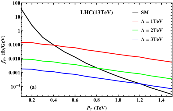
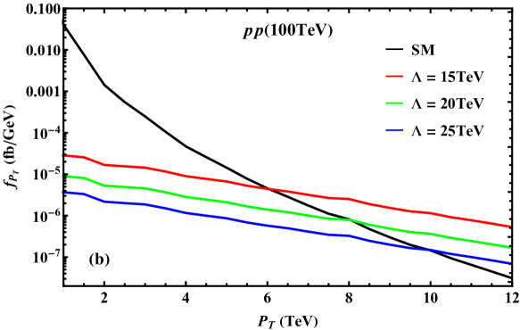
Figure 2: Photon transverse momentum $P_{T}$ distributions at the azimuthal angle $\,\phi_{*}\!=0\,$ for the reaction $\hskip 0.85358ptp{\hskip 0.85358pt}p{\hskip 0.85358pt}(q{\hskip 0.85358pt}\bar{q})\!\rightarrow\!Z\gamma\hskip 0.85358pt$ followed by $\hskip 0.85358ptZ\!\rightarrow\ell\hskip 0.85358pt\bar{\ell}\hskip 0.85358pt$ decays, as contributed by the SM (black curve) and by the nTGC operator $\mathcal{O}_{G+}$ at $O(\Lambda^{-4})$ (colored curves for the indicated values of $\Lambda\hskip 0.85358pt$) at the LHC (13 TeV) in the upper panel and at the 100 TeV $pp$ collider in the lower panel.

According to our definition of the azimuthal angle $\phi_{*}$ in Section 2, we have

$$\cos\phi_{*}\,=\,\frac{\leavevmode\nobreak\ (\mathbf{p}_{q}\!\times\!\mathbf{p}_{Z})\cdot(\mathbf{p}_{f}\!\times\!\mathbf{p}_{\bar{f}})\leavevmode\nobreak\ }{|\mathbf{p}_{q}\!\times\!\mathbf{p}_{Z}|\hskip 0.85358pt|\mathbf{p}_{f}\!\times\!\mathbf{p}_{\bar{f}}|}\,.$$ (4.8)

We note that the quark $q$ can be emitted from either proton beam, so the direction of $\,\mathbf{p}_{q}\,$ is subject to a $180^{\circ}$ ambiguity. This means that the normal direction of the scattering plane of $\hskip 0.85358ptq\hskip 0.85358pt\bar{q}\!\rightarrow\!Z\gamma\hskip 0.85358pt$ is also subject to a $180^{\circ}$ ambiguity, so that $\cos\phi_{*}$ can take either sign in each event and the $\cos\phi_{*}$ terms in $f_{\phi_{*}}^{j}$ cancel out when the statistical average is taken. However, the angular terms $\hskip 0.85358pt\propto\cos(2\hskip 0.85358pt\phi_{*})\!=\!2\cos^{2}\phi_{*}\!-\!1\hskip 0.85358pt$ are not affected by this ambiguity and survive statistical average. Thus, for the nTGC operator $\mathcal{O}_{G+}$ and also the related contact operator $\mathcal{O}_{C-}$, we derive the following effective distributions of $\hskip 0.85358pt\phi_{*}$ after averaging:

$$\bar{f}_{\phi_{*}}^{\hskip 0.85358pt0}\!\! = \!\!\frac{1}{\,2\pi\,}-\frac{\hat{s}\hskip 0.85358ptM_{Z}^{2}\cos 2\phi_{*}\,}{\,2\pi\!\left[(\hat{s}\!-\!M_{Z}^{2})^{2}\!+2(\hat{s}^{2}\!+\!M_{Z}^{4})\ln\sin\!\frac{\delta}{2}\right]\,}+O(\delta)\hskip 0.85358pt,\hskip 11.38109pt$$ (4.9a)

$$\bar{f}_{\phi_{*}}^{\hskip 0.85358pt1}\!\! = \!\!\frac{1}{\,2\pi\,}+\frac{\leavevmode\nobreak\ \hat{s}\cos 2\phi_{*}\leavevmode\nobreak\ }{8\pi M_{Z}^{2}}\hskip 0.85358pt,$$ (4.9b)

$$\bar{f}_{\phi_{*}}^{\hskip 0.85358pt2}\!\! = \!\!\frac{1}{\,2\pi\,}\hskip 0.85358pt.$$ (4.9c)

We see that the interference term $\hskip 0.85358pt\bar{f}_{\phi_{*}}^{\hskip 0.85358pt1}\hskip 0.85358pt$ has a nontrivial angular dependence $\,\propto\cos(2\phi_{*})\hskip 0.85358pt$ that is enhanced by the energy factor $\hskip 0.85358pts/M_{Z}^{2}\hskip 0.85358pt$ relative to the nearly flat SM distribution $\hskip 0.85358pt\bar{f}_{\phi_{*}}^{\hskip 0.85358pt0}\!\!\simeq\!1/2\pi\hskip 0.85358pt$. We present the angular distributions of $\hskip 0.85358pt\phi_{*}\hskip 0.85358pt$ in Fig. 3, where the angular distribution $\hskip 0.85358pt\bar{f}_{\phi_{*}}^{\hskip 0.85358pt1}\hskip 0.85358pt$ (red curve) from the interference contribution of $O(\Lambda^{-4})$ dominates over the nearly flat SM distribution $\hskip 0.85358pt\bar{f}_{\phi_{*}}^{\hskip 0.85358pt0}\hskip 0.85358pt$ (black curve) and the distribution $\hskip 0.85358pt\bar{f}_{\phi_{*}}^{\hskip 0.85358pt2}\hskip 0.85358pt$ (blue curve) of the squared contribution of $O(\Lambda^{-8})$, which is flat and behaves like the SM distribution. In this figure, for illustration we have imposed a selection cut on the parton-parton collision energy, $\sqrt{\hat{s}\,}\!>\!2$ TeV.

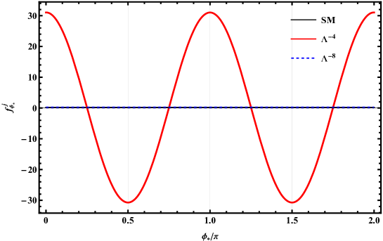
Figure 3: Normalized distributions in the azimuthal angle $\phi_{*}$ for the reaction $\hskip 0.85358ptp{\hskip 0.85358pt}p{\hskip 0.85358pt}(q{\hskip 0.85358pt}\bar{q})\!\rightarrow\!Z\gamma\hskip 0.85358pt$ followed by $Z\!\rightarrow\ell\hskip 0.85358pt\bar{\ell}\hskip 0.85358pt$ decays, as generated by the dimension-8 nTGC operator $\,\mathcal{O}_{G+}$​ at the LHC (13 TeV). The angular distribution $\,f_{\phi_{*}}^{1}$ of the interference contribution of $\hskip 0.85358ptO(\Lambda^{-4})\hskip 0.85358pt$ is shown as a red curve; the angular distribution $\hskip 0.85358ptf_{\phi_{*}}^{2}\hskip 0.85358pt$ of the squared contribution of $\hskip 0.85358pt{\cal O}(\Lambda^{-8})$ is shown as the blue curve that is flat like the SM distribution $\hskip 0.85358ptf_{\phi_{*}}^{0}\hskip 0.85358pt$ (black curve).

For the other operators $\hskip 0.85358pt(\mathcal{O}_{G-},\hskip 0.85358pt\mathcal{O}_{\widetilde{B}W},\hskip 0.85358pt\mathcal{O}_{C+})\hskip 0.85358pt$, inspecting their angular distributions in Eq.(2.17) we find that $(f_{\phi_{*}}^{0},\,f_{\phi_{*}}^{1})$ have the leading energy contributions given by the $\cos\phi_{*}$ terms and the $\hskip 0.85358pt\cos(2\phi_{*})\hskip 0.85358pt$ terms only have subleading energy-dependence. In addition, their contributions to $f_{\phi_{*}}^{2}$ contain no $\hskip 0.85358pt\cos(2\phi_{*})\hskip 0.85358pt$ term. After statistically averaging over the two possible directions of the scattering plane at $pp$ colliders, we derive the following effective distributions:

$$\bar{f}_{\phi_{*}}^{\hskip 0.85358pt0}\!\!\! = \!\!\frac{1}{\,2\pi\,}-\frac{\,\hat{s}\hskip 0.85358ptM_{Z}^{2}\cos 2\phi_{*}\,}{\leavevmode\nobreak\ 2\pi\!\left[(\hat{s}\!-\!M_{Z}^{2})^{2}\!+2(\hat{s}^{2}\!+\!M_{Z}^{4})\ln\sin\frac{\delta}{2}\right]\,}+O(\delta),\hskip 11.38109pt$$ (4.10a)

$$\bar{f}_{\phi_{*}}^{\hskip 0.85358pt1}\!\!\! = \!\!\frac{1}{\,2\pi\,}+\frac{\hat{s}\cos 2\phi_{*}\,}{\leavevmode\nobreak\ 4\pi(\hat{s}\!+\!M_{Z}^{2})\leavevmode\nobreak\ },$$ (4.10b)

$$\bar{f}_{\phi_{*}}^{\hskip 0.85358pt2}\!\!\! = \!\!\frac{1}{\,2\pi\,}\,,$$ (4.10c)

where the SM contribution $\hskip 0.85358pt\bar{f}_{\phi_{*}}^{\hskip 0.85358pt0}$ is the same as that of Eq.(4.9a). For operators $\hskip 0.85358pt(\mathcal{O}_{G-},\hskip 0.85358pt\mathcal{O}_{\widetilde{B}W},\hskip 0.85358pt\mathcal{O}_{C+})\hskip 0.85358pt$, under the statistical average, their angular distribution $f_{\phi_{*}}^{1}$ has a high-energy dependence of $\hskip 0.85358pt\hat{s}^{0}\hskip 0.85358pt$, while the angular distribution $f_{\phi_{*}}^{2}$ becomes a constant and is independent of both the energy and $\phi_{*}$. These should be compared to the statistically averaged angular distributions (4.9b)-(4.9c) for the nTGC operator $\mathcal{O}_{G+}$, where its angular distribution $\hskip 0.85358ptf_{\phi_{*}}^{1}\hskip 0.85358pt$ has higher-energy dependence of $\hskip 0.85358pt\hat{s}^{1}\hskip 0.85358pt$ for the $\hskip 0.85358pt\cos(2\phi_{*})\hskip 0.85358pt$ term, while the angular distribution $f_{\phi_{*}}^{2}$ also becomes constant.

Based on the effective angular distributions (4.9) and Fig. 3, we construct the following observable $\mathbb{O}_{1}$ :

$$\mathbb{O}_{1}\,=\,\left|\hskip 0.85358pt\sigma_{1}\!\int\!\!\mathrm{d}\phi_{*}\,f_{\phi_{*}}^{1}\!\times\text{sign}(\cos 2\phi_{*})\right|,$$ (4.11)

where $\hskip 0.85358pt\sigma_{1}$ is the total cross section from the interference contribution of ${\cal O}(\Lambda^{-4})\hskip 0.85358pt$. Then, we use the formula (4.2) to derive the significance:

$$\mathcal{Z}\,=\,\sqrt{2\!\left(\!B\ln\!\frac{\,B\,}{\,B+S\,}+S\right)}\,=\,\sqrt{2\!\left(\!\sigma_{0}\ln\!\frac{\,\sigma_{0}\,}{\,\sigma_{0}+\mathbb{O}_{1}}+\mathbb{O}_{1}\!\right)}\times\sqrt{\mathcal{L}\times\epsilon\leavevmode\nobreak\ },$$ (4.12)

where $\hskip 0.85358pt\mathcal{L}\hskip 0.85358pt$ is the integrated luminosity and $\hskip 0.85358pt\epsilon\hskip 0.85358pt$ denotes the detection efficiency.

$\sqrt{s\,}$		LHC (13 TeV)			$pp$ (100 TeV)
$\mathcal{L}$ (ab-1)	0.14	0.3	3	3	10	30
$\Lambda_{G+}^{2\sigma}$ (TeV)	2.1	2.4	3.3	14	17	19
$\Lambda_{G+}^{5\sigma}$ (TeV)	1.6	1.8	2.6	10	12	15

Table 2: Sensitivities to the new physics scale $\hskip 0.85358pt\Lambda\hskip 0.85358pt$ at $O(\Lambda^{-4})$ of the nTGC operator $\,\mathcal{O}_{G+}$ at the $2\hskip 0.85358pt\sigma$ and $5\hskip 0.85358pt\sigma$ levels, as obtained by analyzing the reaction $\,p{\hskip 0.85358pt}p{\hskip 0.85358pt}(q{\hskip 0.85358pt}\bar{q})\!\rightarrow\!Z\gamma\!\rightarrow\!\ell\hskip 0.85358pt\bar{\ell}\gamma$  at the LHC (13 TeV) and the $pp$ (100 TeV) collider respectively, with the indicated integrated luminosities.

To achieve the optimal sensitivity, we apply the formula (4.5) to compute the total significance $\mathcal{Z}_{\mathrm{total}}$ from the contributions of the significances $\{\mathcal{Z}_{\mathrm{bin}}\}$ of all the individual bins. In our analysis, we choose the bin size to be $\hskip 0.85358pt\Delta P_{T}\!=\!100$ GeV for the LHC (13 TeV) and $\Delta P_{T}\!=\!500$ GeV for the $pp{\hskip 0.85358pt}$(100 TeV) collider. But we find that $\hskip 0.85358pt\mathcal{Z}_{\mathrm{total}}$ is not very sensitive to such choice. For instance, if we choose $\Delta P_{T}\!=\!50$ GeV or $\Delta P_{T}\!=\!200$ GeV at the LHC, we find that the significance $\hskip 0.85358pt\mathcal{Z}_{\mathrm{total}}$ only varies by about 1% .

We present prospective sensitivity reaches for probing the new physics scale $\Lambda$ of the nTGC operator $\mathcal{O}_{G+}$ in Table 2. For instance, given an integrated luminosity $\,\mathcal{L}\!=\!300\,$fb^-1 ($3\,$ab^-1) at the LHC and choosing the ideal detection efficiency $\epsilon\!=\!1\hskip 0.85358pt$, we find the $2{\hskip 0.85358pt}\sigma$ sensitivity reach $\,\Lambda_{G+}^{2\sigma}\!\simeq\!2.6$ TeV ($\,\Lambda_{G+}^{2\sigma}\!\simeq\!3.6$ TeV). At the 100 TeV $pp$ collider with $\mathcal{L}\!=\!3$ ab^-1 (30 ab^-1), we derive the $2{\hskip 0.85358pt}\sigma$ sensitivity reach $\,\Lambda_{G+}^{2\sigma}\!\simeq\!15$ TeV ($\hskip 0.85358pt\Lambda_{G+}^{2\sigma}\!\simeq 21$ TeV ).

4.3 nTGC Analysis Including ${\cal O}(\Lambda^{\!-8})$ Contributions

In this subsection, we further analyze the squared contributions of $\mathcal{O}(\Lambda^{\!-8})$ and study their impact on the sensitivity reaches at the LHC and the $pp\hskip 0.85358pt$(100 TeV) collider. Inspecting the effective angular distributions (4.9), we find that requiring the differential cross section of the interference contribution of $\mathcal{O}(\Lambda^{\!-4})$ to be larger than that of the squared contribution of $\mathcal{O}(\Lambda^{\!-8})$ would impose the following condition:

$$\left|\sigma_{1}f^{1}_{\phi_{*}}\right|\,>\,\sigma_{2}f^{2}_{\phi_{*}}\!=\!\frac{\sigma_{2}}{\leavevmode\nobreak\ 2\pi\leavevmode\nobreak\ }\,,$$ (4.13)

which gives a lower bound of $\,\Lambda\!>\!1.3\sqrt{\hat{s}\,}\,$ for the reaction channel $\,u\hskip 0.85358pt\bar{u}\!\rightarrow\!Z\gamma\,$ and $\,\Lambda\!>\!1.5\sqrt{\hat{s}\,}\,$ for the $d\bar{d}\!\rightarrow\!Z\gamma\,$ channel. These bounds are comparable or somewhat stronger than the LHC sensitivity limits of the new physics scale $\hskip 0.85358pt\Lambda\hskip 0.85358pt$ given in Table 2, whereas they are satisfied by the sensitivity limits of the 100 TeV $pp$ collider. Thus, to improve the sensitivities for the LHC probe of the nTGCs, we consider the full contributions of the nTGC operators including their squared terms of ${\cal O}(\Lambda^{\!-8})$. We note that including the full contributions of the nTGC operators also allows a consistent mapping of the current analysis to the form factor approach given in the following Section 4.5 which always includes the full contributions of the form factors to the cross sections.

We present in Fig. 4 the photon $P_{T}$ distribution including the contribution of ${\cal O}(\Lambda^{\!-8})$. Since the ${\cal O}(\Lambda^{\!-8})$ contribution can be larger than ${\cal O}(\Lambda^{\!-4})$ for large $\hat{s\,}$, we choose here a set of larger values $\,\Lambda\!=\!(2,4,6)$ TeV for the LHC distributions and $\,\Lambda\!=\!(20,25,30)$ TeV for the distributions at the $pp\hskip 0.85358pt$(100 TeV) collider, instead of the previous values of $\,\Lambda\!=\!(1,2,3)$ TeV for the LHC and $\,\Lambda\!=\!(15,20,25)$ TeV for the $pp\hskip 0.85358pt$(100 TeV) collider chosen for Fig.2. Also, Fig. 4 extends to a larger range of the photon $P_{T}$ .

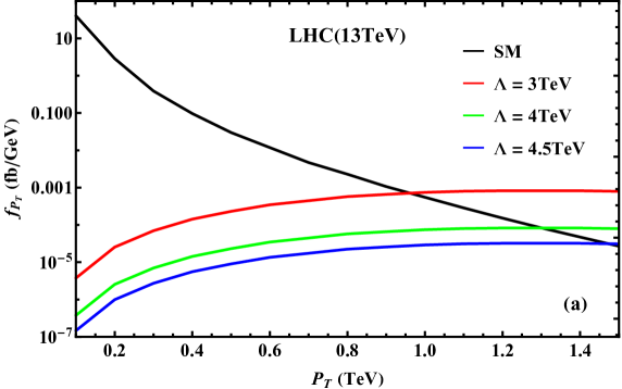
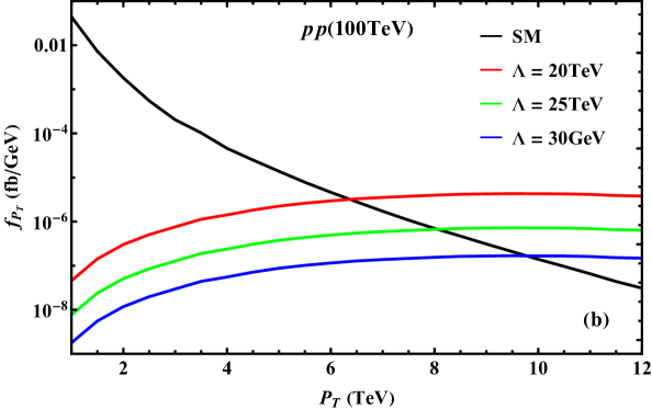
Figure 4: Photon transverse momentum $P_{T}$ distributions at the azimuthal angle $\phi_{*}\!=\!0$ for the reaction $\hskip 0.85358ptp{\hskip 0.85358pt}p{\hskip 0.85358pt}(q{\hskip 0.85358pt}\bar{q})\!\rightarrow\!Z\gamma\hskip 0.85358pt$ followed by $\hskip 0.85358ptZ\!\rightarrow\ell\bar{\ell}\hskip 0.85358pt$ decays, as contributed by the SM (black curve) and by the nTGC operator $\mathcal{O}_{G+}$ up to $\hskip 0.85358pt{O}(\Lambda^{-4})$ and $\hskip 0.85358pt{O}(\Lambda^{-8})$ (colored curves) at the LHC (13 TeV) and the $pp$ (100 TeV) collider in the lower panel.

For the high-energy hadron colliders such as the LHC and $pp\hskip 0.85358pt$(100 TeV), we have $\hskip 0.85358pt|\sigma_{1}|\ll 2\pi|\sigma_{1}f^{1}_{\phi_{*}}|\!<\!\sigma_{2}\hskip 0.85358pt$, and thus $\sigma_{1}$ may be neglected. Following the procedure in Section 4.2, we use the same method and cuts on $P_{T}$ to divide events into a set of bins. Because the $\phi_{*}$ distribution is rather flat for both the SM and $O(\Lambda^{-8})$ contributions, we do not need to impose an angular cut on $\phi_{*}\hskip 0.85358pt$. We analyze the sensitivity reaches of $\hskip 0.85358pt\Lambda\hskip 0.85358pt$ by using Eq.(4.5), and present the results for probing the nTGC operator $\hskip 0.85358pt\mathcal{O}_{G+}\hskip 0.85358pt$ up to ${\cal O}(\Lambda^{\!-8})$ in Table 3. The sensitivity reaches at ${\cal O}(\Lambda^{\!-8})$ appear significantly better than those at ${\cal O}(\Lambda^{\!-4})$ shown in Table 2.

For instance, given an integrated luminosity $\,\mathcal{L}\!=\!300\,$fb^-1 ($3\,$ab^-1) at the LHC and choosing the ideal detection efficiency $\epsilon\!=\!1\hskip 0.85358pt$, we find from Table 3 that the $2{\hskip 0.85358pt}\sigma$ sensitivity reach is given by $\,\Lambda_{G+}^{2\sigma}\!\!\simeq\!3.4$ TeV ($\,\Lambda_{G+}^{2\sigma}\!\!\simeq\!4.1$ TeV). At the 100 TeV $pp$ collider with $\mathcal{L}\!\!=\!3$ ab^-1 (30 ab^-1), we obtain the $2{\hskip 0.85358pt}\sigma$ sensitivity reach $\,\Lambda_{G+}^{2\sigma}\!\simeq\!22$ TeV ($\hskip 0.85358pt\Lambda_{G+}^{2\sigma}\!\simeq 27$ TeV ).

$\sqrt{s\,}$		LHC (13 TeV)			$pp$ (100 TeV)
$\mathcal{L}$ (ab-1)	0.14	0.3	3	3	10	30
$\Lambda_{G+}^{2\sigma}$ (TeV)	3.0	3.2	3.9	21	24	26
$\Lambda_{G+}^{5\sigma}$ (TeV)	2.6	2.8	3.4	17	20	22

Table 3: Sensitivities to the new physics scale $\Lambda$ at $O(\Lambda^{-8})$ of the nTGC operator $\,\mathcal{O}_{G+}$ at the $2\hskip 0.85358pt\sigma$ and $5\hskip 0.85358pt\sigma$ levels, as obtained by analyzing the reaction $\,p{\hskip 0.85358pt}p{\hskip 0.85358pt}(q{\hskip 0.85358pt}\bar{q})\!\rightarrow\!Z\gamma\!\rightarrow\!\ell\bar{\ell}\gamma$  at the LHC (13 TeV) and the $pp\hskip 0.85358pt$(100 TeV) collider respectively, with the indicated integrated luminosities.

$\sqrt{s\,}$		LHC (13  TeV)			$pp$ (100 TeV)
$\mathcal{L}$ (ab-1)	0.14	0.3	3	3	10	30
$\Lambda_{G+}^{2\sigma}$ (TeV)	3.3	3.6	4.2	23	26	28
$\Lambda_{G+}^{5\sigma}$ (TeV)	2.9	3.1	3.7	20	22	24

Table 4: Sensitivity reaches on the new physics scale $\Lambda$ at $O(\Lambda^{-8})$ of the nTGC operator $\,\mathcal{O}_{G+}$ at the $2{\hskip 0.85358pt}\sigma$ and $5{\hskip 0.85358pt}\sigma$ levels, as obtained from the reactions $\,p{\hskip 0.85358pt}p{\hskip 0.85358pt}(q{\hskip 0.85358pt}\bar{q})\!\rightarrow\!Z\gamma\!\rightarrow\!\ell\bar{\ell}\gamma$  and $\,p{\hskip 0.85358pt}p{\hskip 0.85358pt}(q{\hskip 0.85358pt}\bar{q})\!\rightarrow\!Z\gamma\!\rightarrow\!\nu\bar{\nu}\gamma$ at the LHC (13 TeV) and the $pp$ (100 TeV) collider, with the indicated integrated luminosities.

$\sqrt{s\,}$		13 TeV ($\ell\hskip 0.85358pt\bar{\ell}$)			13 TeV ($\ell\hskip 0.85358pt\bar{\ell},\nu\bar{\nu}$)			100 TeV ($\ell\hskip 0.85358pt\bar{\ell}$)			100 TeV ($\ell\hskip 0.85358pt\bar{\ell},\nu\bar{\nu}$)
$\mathcal{L}$(ab-1)	0.14	0.3	3	0.14	0.3	3	3	10	30	3	10	30
$\Lambda_{\widetilde{B}W}$ (TeV)	1.2	1.3	1.5	1.3	1.4	1.7	5.1	5.6	6.1	5.6	6.1	6.7
$\Lambda_{G-}$ (TeV)	1.0	1.1	1.3	1.1	1.2	1.4	4.2	4.7	5.1	4.6	5.1	5.5
$\Lambda_{C+}$ (TeV)	1.3	1.4	1.6	1.4	1.5	1.7	5.4	5.9	6.5	5.9	6.5	7.1

Table 5: Sensitivity reaches on the new physics scales of the nTGC operators $\hskip 0.85358pt(\mathcal{O}_{\widetilde{B}W},\hskip 0.85358pt\mathcal{O}_{G-},\hskip 0.85358pt\mathcal{O}_{C+})\hskip 0.85358pt$ at the $2\hskip 0.85358pt\sigma$ level, as obtained from analyzing the reactions $\,p{\hskip 0.85358pt}p{\hskip 0.85358pt}(q{\hskip 0.85358pt}\bar{q})\!\rightarrow\!Z\gamma\!\rightarrow\!\ell\bar{\ell}\gamma$ and $\,p{\hskip 0.85358pt}p{\hskip 0.85358pt}(q{\hskip 0.85358pt}\bar{q})\!\rightarrow\!Z\gamma\!\rightarrow\!\nu\bar{\nu}\gamma$ at the LHC (13 TeV) and the $pp$ (100 TeV) collider, with the indicated integrated luminosities. The third and fifth columns indicated by ($\hskip 0.85358pt\ell\hskip 0.85358pt\bar{\ell},\hskip 0.85358pt\nu\hskip 0.85358pt\bar{\nu}$) present the combined limits including both the charged-lepton and neutrino final states.

4.4 nTGC Analysis Including the Invisible Decays $Z\!\rightarrow\!\nu\bar{\nu}$

In this subsection, we study the probe of nTGCs via the $Z\gamma$ production with invisible decays $\hskip 0.85358ptZ\!\!\rightarrow\!\!\nu\hskip 0.85358pt\bar{\nu}\hskip 0.85358pt$. In this case, the final-state photon is the only signature of $Z\gamma$ production that can be detected, and we will use the jet-vetoing to effectively remove all the reducible SM backgrounds having the final state  jet$+\gamma\hskip 0.85358pt$. Then, we can use the same strategy as that for probing the ${\cal O}(\Lambda^{-8})$ contribution via the leptonic $Z$-decay channels, where the kinetic cut on the photon $P_{T}$ distribution will play the major role to enhance the sensitivity to the nTGC contributions.

Following this strategy, we perform combined analyses for both the $\hskip 0.85358ptZ\!\!\rightarrow\!\ell\hskip 0.85358pt\bar{\ell}\,$ final state and the $Z\!\!\rightarrow\!\nu\hskip 0.85358pt\bar{\nu}\,$ final state. We present in Table 4 a summary of the prospective sensitivity reaches on the new physics scale $\hskip 0.85358pt\Lambda\hskip 0.85358pt$ of the nTGC operator $\hskip 0.85358pt\mathcal{O}_{G+}\hskip 0.85358pt$, where we have combined the limits from both the charged-lepton final state and the neutrino final state. We find that the combination of both leptonic and invisible $Z$-decay channels can enhance the sensitivity to the new physics scale $\hskip 0.85358pt\Lambda\hskip 0.85358pt$ by about 10% over that using the leptonic channels alone.

Using the sensitivity bounds of Table 4 and comparing them with our study for $e^{+}e^{-}$ colliders [5] (which will be summarized later in Table 9 of Section 5), we find that for probing the nTGC operator $\mathcal{O}_{G+}$ the sensitivity reaches with the current LHC luminosity ($\hskip 0.85358pt\mathcal{L}=140\,$fb^-1) are already better than those at future 250 GeV and 500 GeV $e^{+}e^{-}$ colliders [5], and that the HL-LHC (with $\hskip 0.85358pt\mathcal{L}\!=\!3\hskip 0.85358pt$ab^-1) should have comparable sensitities to a 1 TeV $e^{+}e^{-}$ collider [5]. The future $pp$ (100 TeV) collider can have much stronger sensitivities than an ($3\!-\!5$) TeV $e^{+}e^{-}$ collider. A systematic comparison with the high-energy $e^{+}e^{-}$ colliders will be presented in the following Section 5.

Next, we extend the above analysis to the three other nTGC operators $\hskip 0.85358pt(\mathcal{O}_{G-},\hskip 0.85358pt\mathcal{O}_{\widetilde{B}W},\hskip 0.85358pt\mathcal{O}_{C+})\hskip 0.85358pt$. We present the 2$\hskip 0.85358pt\sigma$ sensitivities to their associated new physics scales in Table 5. The third and fifth columns of this Table, marked with ($\ell\hskip 0.85358pt\bar{\ell},\nu\hskip 0.85358pt\bar{\nu}$), present the combined limits including both the charged-lepton and neutrino final states. We see that these sensitivities are significantly weaker than those of the operators $\hskip 0.85358pt\mathcal{O}_{G+}\hskip 0.85358pt$ and $\hskip 0.85358pt\mathcal{O}_{C-}\hskip 0.85358pt$. At the LHC, they are generally below 2 TeV, but the proposed 100 TeV $pp$ collider could improve the sensitivities substantially, reaching new physics scales $\hskip 0.85358pt\Lambda\hskip 0.85358pt$ over the $(5-7)$ TeV range. Finally, we compare the collider sensitivity limits presented in Tables 3-5 with the perturbative unitarity limits given in Table 1 and Fig. 1. We find that our collider limits are much stronger than the unitarity limits of Table 1 and Fig. 1. Hence, our current collider analyses of probing the nTGCs via the SMEFT formulation hold well the perturbation expansion.

Operators	$\mathcal{O}^{(3)}_{L}(q_{L})$	$\mathcal{O}_{L}(q_{L})$	$\mathcal{O}_{R}(u_{R})$	$\mathcal{O}_{R}(d_{R})$
$\Lambda\hskip 0.85358pt$[PDG] (TeV)	4.7	4.7	2.9	2.4
$\Lambda\hskip 0.85358pt$[CEPC] (TeV)	9.1	9.1	5.5	5.1

Table 6: Precision constraints at the $\hskip 0.85358pt2\sigma$ level on the indicated dimension-6 operators that contribute to the $q$-$\bar{q}$-$Z$ coupling. The bounds $\Lambda\hskip 0.85358pt$[PDG] are derived from the existing electroweak data [31], whereas the bounds $\Lambda\hskip 0.85358pt$[CEPC] are the projected sensitivities of the future $e^{+}e^{-}$ collider CEPC ($250\hskip 0.85358pt$GeV) [30].

As a final remark, we emphasize that the reaction $\hskip 0.85358ptq\bar{q}\!\rightarrow\!Z\gamma\,$ is a unique process for probing the nTGCs via $s$-channel at the LHC and future $pp$ colliders. We note, however, that certain dimension-6 operators can contribute to the process $q\bar{q}\!\rightarrow\!Z\gamma$ via $t$-channel diagrams by modifying the $q$-$\bar{q}$-$Z$ vertex. Such contributions are constrained separately by existing electroweak precision data via other reactions, and future $e^{+}e^{-}$ colliders will place more severe constraints on the $q$-$\bar{q}$-$Z$ coupling via $Z$-pole measurements. These measurements are independent of the reaction $\,q\bar{q}\!\rightarrow\!Z\gamma\,$, and may be obtained from global fits to $(\alpha,\hskip 0.85358ptG_{F},\hskip 0.85358ptM_{Z},\hskip 0.85358ptM_{W})$ and other $Z$-pole observables [29][30][31]. We take values of these observables from the current electroweak precision data [31] and from the projected CEPC sensitivities [30]. For contributions to the $q$-$\bar{q}$-$Z$ coupling, we consider the following dimension-6 Higgs-related operators:

$$\mathcal{O}^{(3)}_{L} =\,(\text{i}H^{\dagger}\sigma^{a}\!\!\stackrel{{\scriptstyle\leftrightarrow}}{{D}}_{\mu}\!\!H)(\overline{\Psi}_{L}\gamma^{\mu}\sigma^{a}\Psi_{L})\hskip 0.85358pt,$$

$$\mathcal{O}_{L} =\,(\text{i}H^{\dagger}\!\stackrel{{\scriptstyle\leftrightarrow}}{{D}}_{\mu}\!H)(\overline{\Psi}_{L}\gamma^{\mu}\Psi_{L})\hskip 0.85358pt,$$ (4.14)

$$\mathcal{O}_{R} =\,(\text{i}H^{\dagger}\!\!\stackrel{{\scriptstyle\leftrightarrow}}{{D}}_{\mu}\!\!H)(\overline{\psi}_{R}\gamma^{\mu}\psi_{R})\hskip 0.85358pt.$$

Then, using the method of [30] we make a global fit and obtain the electroweak precision constraints on the cutoff scale $\Lambda$ of these operators, which we summarize in Table 6, assuming for simplicity that the dimension-6 operators are universal for the three families of fermions. Table 6 shows that the dimension-6 operators (4.14) can be constrained independently through different processes and observables. The existing bounds $\Lambda\hskip 0.85358pt$[PDG] derived in Table 6 are already strong and the projected sensitivities on the cutoff scale $\Lambda\hskip 0.85358pt$[CEPC] for the future $e^{+}e^{-}$ collider CEPC ($250\hskip 0.85358pt$GeV) are much stronger than the corresponding bounds on the cutoff scale of the dimension-8 nTGC operators at the same $e^{+}e^{-}$ collider (as we show below in Table 9 of Section 5).

4.5 Probing the Form Factors of nTGVs

In this Section we analyze the sensitivity reaches of the LHC and the $pp$ (100 TeV) collider for probing the nTGCs by using the form factor formulation given in Section 3. We will also clarify the nontrivial difference between our consistent form factor formulation (3.5) (based upon the fully gauge-invariant SMEFT approach) and the conventional form factor formulation (3.1) [retaining only the residual gauge symmetry U(1)${}_{\mathrm{em}}\hskip 0.85358pt$], where the latter leads to erroneously strong sensitivity limits.

From Eqs.(2.2), (2.2)-(2.16) and (3.6), we can further derive the partonic cross section of the reaction $\,q\hskip 0.85358pt\bar{q}\!\rightarrow\!Z\gamma\hskip 0.85358pt$ in terms of the form factors. As before, we decompose the partonic cross section into the sum of three parts, $\,\sigma(Z\gamma)=\sigma_{0}+\sigma_{1}+\sigma_{2}\,$, where $(\sigma_{0},\hskip 0.85358pt\sigma_{1},\hskip 0.85358pt\sigma_{2})$ correspond to the SM contribution, the interference contribution, and the squared contribution, respectively. The cross section terms $(\sigma_{1},\hskip 0.85358pt\sigma_{2})$ are contributed by the form factors and take the following expressions:

$$\sigma_{1}\!\! = \!\!-\frac{\,e^{2}Qq_{L}\hskip 0.85358pt{T_{3}}\!\left(\hat{s}\!-\!M_{Z}^{2}\right)\,}{4\pi v^{2}\,\hat{s}}h_{4}-\frac{\,e^{2}Q(q_{L}x_{L}^{Z}\!\!-\!q_{R}x_{R}^{Z})(\hat{s}^{2}\!-\!M_{Z}^{4})\,}{\,4\pi v^{2}\hskip 0.85358pt\hat{s}^{2}\,}h_{3}^{Z}$$ (4.15)

$$+\frac{\,e^{2}c_{W}Q(q_{L}x_{L}^{A}\!\!-\!q_{R}x_{R}^{A})(\hat{s}^{2}\!-\!M_{Z}^{4})\,}{\,4\pi s_{W}v^{2}\hskip 0.85358pt\hat{s}^{2}\,}h_{3}^{\gamma}\,,\hskip 28.45274pt$$

and

$$\sigma_{2}\!\! = \!\!\sigma_{2}^{44}+\sigma_{2Z}^{33}+\sigma_{2A}^{33}+\sigma_{2Z}^{43}+\sigma_{2A}^{43}+\sigma_{2ZA}^{33}\,,$$ (4.16a)

$$\sigma_{2}^{44}\!\! = \!\!\frac{\leavevmode\nobreak\ e^{4}T_{3}^{2}(\hat{s}+\!M_{Z}^{2})(\hat{s}-\!M_{Z}^{2}){}^{3}\leavevmode\nobreak\ }{\leavevmode\nobreak\ 768\hskip 0.85358pt\pi s_{W}^{2}c_{W}^{2}M_{Z}^{8}\,\hat{s}\leavevmode\nobreak\ }(h_{4})^{2}\,,$$ (4.16b)

$$\sigma_{2Z}^{33}\!\! = \!\!\frac{\leavevmode\nobreak\ e^{4}[Q^{2}s_{W}^{4}\!+\!(T_{3}\!-Qs_{W}^{2})^{2}](\hat{s}\!+\!M_{Z}^{2})(\hat{s}\!-\!M_{Z}^{2})^{3}\,}{\leavevmode\nobreak\ 192\hskip 0.85358pt\pi\hskip 0.85358pts_{W}^{2}c_{W}^{2}M_{Z}^{6}\,\hat{s}^{2}\leavevmode\nobreak\ }(h_{3}^{Z})^{2}\,,$$ (4.16c)

$$\sigma_{2A}^{33}\!\! = \!\!\frac{\leavevmode\nobreak\ e^{4}Q^{2}(\hat{s}\!+\!M_{Z}^{2})(\hat{s}\!-\!M_{Z}^{2})^{3}\,}{96\hskip 0.85358pt\pi M_{Z}^{6}\,\hat{s}^{2}}(h_{3}^{\gamma})^{2}\,,$$ (4.16d)

$$\sigma_{2Z}^{43}\!\! = \!\!\frac{\leavevmode\nobreak\ e^{4}T_{3}(T_{3}\!-\!Qs_{W}^{2})(\hat{s}\!-\!M_{Z}^{2})^{3}\,}{96\hskip 0.85358pt\pi\hskip 0.85358pts_{W}^{2}c_{W}^{2}M_{Z}^{6}\,\hat{s}}h_{4}h_{3}^{Z}\,,$$ (4.16e)

$$\sigma_{2A}^{43}\!\! = \!\!\frac{\leavevmode\nobreak\ e^{4}Q\hskip 0.85358ptT_{3}\hskip 0.85358pt(\hat{s}\!-\!M_{Z}^{2})^{3}\,}{\leavevmode\nobreak\ 96\hskip 0.85358pt\pi\hskip 0.85358pts_{W}c_{W}M_{Z}^{6}\,\hat{s}\leavevmode\nobreak\ }h_{4}h_{3}^{\gamma}\,,$$ (4.16f)

$$\sigma_{2ZA}^{33}\!\! = \!\!\frac{\leavevmode\nobreak\ e^{4}Q(T_{3}\!-\!2Qs_{W}^{2})(\hat{s}\!+\!M_{Z}^{2})(\hat{s}\!-\!M_{Z}^{2})^{3}\,}{\leavevmode\nobreak\ 96\hskip 0.85358pt\pi\hskip 0.85358pts_{W}c_{W}M_{Z}^{6}\,\hat{s}^{2}\leavevmode\nobreak\ }h_{3}^{Z}h_{3}^{\gamma}\,,$$ (4.16g)

where the coefficients $(q_{L},\,q_{R})\!=\!(T_{3}\!-\!Qs_{W}^{2},\hskip 0.85358pt-Qs_{W}^{2})$ denote the (left, right)-handed gauge couplings between the quarks and $Z$ boson. The form factor $\,h_{3}^{Z}$ is contributed by the operator $\mathcal{O}_{\widetilde{B}W}$ as in Eq.(3.6b) and the coupling coefficients $(x_{L}^{Z},\hskip 0.85358ptx_{R}^{Z})\!=\!(T_{3}\!-\!Qs_{W}^{2},\hskip 0.85358pt-Qs_{W}^{2})$ are given by Eq.(2.16b), whereas the form factor $\,h_{3}^{\gamma}$ is contributed by the operator $\mathcal{O}_{G-}$ as in Eq.(3.6c) and the coupling coefficients $(x_{L}^{A},\hskip 0.85358ptx_{R}^{A})\!=\!-Qs_{W}^{2}(1,\hskip 0.85358pt1)$ are given by Eq.(2.16a). Inspecting Eqs.(4.15)-(4.16), we find that the cross section terms $(\sigma_{1},\hskip 0.85358pt\sigma_{2})$ have the following scaling behaviors in the high energy limit:

$$\sigma_{1} =\,O(\hat{s}^{0})\hskip 0.85358pth_{4}+O(\hat{s}^{0})\hskip 0.85358pth_{3}^{Z}+O(\hat{s}^{0})\hskip 0.85358pth_{3}^{\gamma}\,,$$ (4.17a)

$$\sigma_{2} =\,O(\hat{s}^{3})(h_{4})^{2}+O(\hat{s}^{2})(h_{3}^{V})^{2}+O(\hat{s}^{2})(h_{4}h_{3}^{V})+O(\hat{s}^{2})(h_{3}^{Z}h_{3}^{\gamma})\,,$$ (4.17b)

where we have used the notation $V\!=\!Z,\gamma\hskip 1.42262pt$.

If we consider instead the conventional parametrization (3.1) with the nTGC form factors $(h_{3}^{V},\hskip 0.85358pth_{4}^{V})$ only, we would obtain their contributions to the total cross section $\,\widetilde{\sigma}(Z\gamma)\!=\sigma_{0}+\widetilde{\sigma}_{1}+\widetilde{\sigma}_{2}\,$. The form factors $h_{3}^{V}$ are not subject to the constraints (3.4) imposed by the dimension-8 nTGC operators of the SMEFT, so they contribute to $(\hskip 0.85358pt\widetilde{\sigma}_{1},\hskip 0.85358pt\widetilde{\sigma}_{2})$ in the same way as in our Eqs.(4.15)-(4.16). However, the $h_{4}^{V}$ contributions to the interference and squared cross sections $(\hskip 0.85358pt\widetilde{\sigma}_{1},\hskip 0.85358pt\widetilde{\sigma}_{2})$ have vital differences from Eqs.(4.15)-(4.17). For simplicity of illustration, we set $\hskip 0.85358pth_{3}^{V}\!=0\hskip 0.85358pt$ and express the $h_{4}^{V}$ contributions to $(\hskip 0.85358pt\widetilde{\sigma}_{1},\hskip 0.85358pt\widetilde{\sigma}_{2})$ as follows:

$$\widetilde{\sigma}_{1}(h_{4}^{V}) =\frac{\,e^{4}Q(\hat{s}\!-\!M_{Z}^{2})^{2}\!\,}{\leavevmode\nobreak\ 32\hskip 0.85358pt\pi\hskip 0.85358pts_{W}^{2}c_{W}^{2}M_{Z}^{4}\,\hat{s}\leavevmode\nobreak\ }\!\left[(q_{L}x_{L}^{Z}\!\!-\!q_{R}x_{R}^{Z})h_{4}^{Z}-(q_{L}x_{L}^{A}\!\!-\!q_{R}x_{R}^{A})\frac{c_{W}}{s_{W}}h_{4}^{\gamma}\right]\!,$$ (4.18a)

$$\widetilde{\sigma}_{2}(h_{4}^{V}) =\frac{e^{4}(\hat{s}\!-\!M^{2}_{Z})^{5}\,}{\leavevmode\nobreak\ 768\hskip 0.85358pt\pi\hskip 0.85358pts_{W}^{2}c_{W}^{2}M_{Z}^{10}\,\hat{s}\leavevmode\nobreak\ }\!\!\left[X_{LR}^{ZZ}(h_{4}^{Z})^{2}+X_{LR}^{AA}\frac{c_{W}^{2}}{s_{W}^{2}}(h_{4}^{\gamma})^{2}-2X_{LR}^{ZA}\frac{c_{W}}{s_{W}}(h_{4}^{Z}h_{4}^{\gamma})\right]\!,$$ (4.18b)

where we have defined the notations

$$X_{LR}^{ZZ}\equiv(x_{L}^{Z})^{2}+(x_{R}^{Z})^{2},\leavevmode\nobreak\ \leavevmode\nobreak\ \leavevmode\nobreak\ X_{LR}^{AA}\equiv(x_{L}^{A})^{2}+(x_{R}^{A})^{2},\leavevmode\nobreak\ \leavevmode\nobreak\ \leavevmode\nobreak\ X_{LR}^{ZA}\equiv x_{L}^{Z}x_{L}^{A}+x_{R}^{Z}x_{R}^{A}\,.$$ (4.19)

Taking the high-energy limit, we find that the cross sections $(\hskip 0.85358pt\widetilde{\sigma}_{1},\hskip 0.85358pt\widetilde{\sigma}_{2})$ scale as follows:

$$\widetilde{\sigma}_{1}(h_{4}^{V}) =\,O(\hat{s})\hskip 0.85358pth_{4}^{Z}+O(\hat{s})\hskip 0.85358pth_{4}^{\gamma}\,,$$ (4.20a)

$$\widetilde{\sigma}_{2}(h_{4}^{V}) =\,O(\hat{s}^{4})(h_{4}^{Z})^{2}+O(\hat{s}^{4})(h_{4}^{\gamma})^{2}+O(\hat{s}^{4})(h_{4}^{Z}h_{4}^{\gamma})\,.$$ (4.20b)

Comparing Eq.(4.20) with Eq.(4.17), we see that the $h_{4}^{V}$ contributions to the cross sections $(\hskip 0.85358pt\widetilde{\sigma}_{1},\hskip 0.85358pt\widetilde{\sigma}_{2})$ in the conventional form factor parametrization (3.1) have an additional high-energy factor of $s^{1}$ beyond the $h_{4}$ contributions to $(\sigma_{1},\hskip 0.85358pt\sigma_{2})$ in our improved parametrization (3.5).

$\sqrt{s\,}$		13 TeV ($\ell\hskip 0.85358pt\bar{\ell}$)			13 TeV ($\ell\hskip 0.85358pt\bar{\ell},\nu\bar{\nu}$)
$\mathcal{L}$(ab-1)	0.14	0.3	3	0.14	0.3	3
$|h_{4}(\hskip 0.85358pt\mathbb{O}_{1})|\!\times\!10^{5}$	5.8 (18)	3.7 (11)	1.0 (2.8)	5.8 (18)	3.7 (11)	1.0 (2.8)
$|h_{4}|\!\times\!10^{6}$	14 (28)	11 (21)	5.2 (9.1)	9.6 (18)	7.5 (14)	3.8 (6.4)
$|h_{3}^{Z}|\!\times\!10^{4}$	2.7 (5.0)	2.1 (3.8)	1.1 (1.8)	1.9 (3.4)	1.5 (2.7)	0.80 (1.3)
$|h_{3}^{\gamma}|\!\times\!10^{4}$	3.1 (5.8)	2.5 (4.5)	1.3 (2.1)	2.2 (4.0)	1.8 (3.1)	0.97 (1.6)
$\sqrt{s\,}$		100 TeV ($\ell\hskip 0.85358pt\bar{\ell}$)			100 TeV ($\ell\hskip 0.85358pt\bar{\ell},\nu\bar{\nu}$)
$\mathcal{L}$(ab-1)	3	10	30	3	10	30
$|h_{4}(\hskip 0.85358pt\mathbb{O}_{1})|\!\times\!{\hskip 0.85358pt10^{8}}$	3.4 (11)	1.6 (5.0)	0.85 (2.6)	3.4 (11)	1.6 (5.0)	0.85 (2.6)
$|h_{4}|\!\times\!10^{9}$	6.1 (13)	3.9 (7.8)	2.6 (5.1)	4.0 (8.1)	2.6 (5.1)	1.9 (3.4)
$|h_{3}^{Z}|\!\times\!10^{7}$	8.9 (17)	6.0 (11)	4.2 (7.5)	6.1 (11)	4.2 (7.5)	3.0 (5.2)
$|h_{3}^{\gamma}|\!\times\!10^{7}$	10 (20)	6.8 (13)	4.9 (8.7)	7.2 (13)	4.9 (8.7)	3.5 (6.1)

Table 7: Sensitivity reaches on the nTGC form factor parameters at the $2\hskip 0.85358pt\sigma$ (black color) and $5\hskip 0.85358pt\sigma$ (blue color) levels, as derived by analyzing the reactions $\,p{\hskip 0.85358pt}p{\hskip 0.85358pt}(q{\hskip 0.85358pt}\bar{q})\!\rightarrow\!Z\gamma\!\rightarrow\!\ell\bar{\ell}\gamma$  and $\,p{\hskip 0.85358pt}p{\hskip 0.85358pt}(q{\hskip 0.85358pt}\bar{q})\!\rightarrow\!Z\gamma\!\rightarrow\!\nu\bar{\nu}\gamma$ at the LHC (13 TeV) and the $pp$ (100 TeV) collider, with the indicated integrated luminosities. In the third and ninth rows, the sensitivity limits for $|h_{4}(\hskip 0.85358pt\mathbb{O}_{1})|$ are derived by using the observable (4.11) from the interference contributions, whereas the $|h_{4}|$ limits in the fourth and tenth rows are derived including the squared contributions. The third and fifth columns marked ($\hskip 0.85358pt\ell\hskip 0.85358pt\bar{\ell},\hskip 0.85358pt\nu\hskip 0.85358pt\bar{\nu}$) present the combined limits including both the charged-lepton and neutrino final states.

We present in Table 7 the sensitivities of probes of the form factor parameters $h_{i}^{V}$ at the LHC (13 TeV) and a 100 TeV $pp$ collider (marked in blue), with the indicated integrated luminosities. We recall that the form factors and dimension-8 operators are connected via Eq.(3.6). We find that the most sensitive probes are those of the form factor $\hskip 0.85358pth_{4}\hskip 0.85358pt$, which is generated by the nTGC operator $\mathcal{O}_{G+}$. The sensitivities of probes of $h_{3}^{Z}$ (via the operator $\mathcal{O}_{\widetilde{B}W}$) and $h_{3}^{\gamma}$ (via the operator $\mathcal{O}_{G-}$) are smaller. In the case of $h_{4}$, we present in the third row the sensitivities obtained from the interference contributions using the observable $\mathbb{O}_{1}$ of Eq.(4.11), and in the fourth row the sensitivities from the squared contributions. The sensitivity limits in the third row are not improved by including the invisible decays of $Z\!\rightarrow\!\nu{\hskip 0.85358pt}\bar{\nu}$ because the angular distribution of $\phi_{*}$ cannot be measured for the invisible channel. We see that the sensitivity bounds on $|h_{4}|$ in the fourth row are significantly stronger than those in the third row. This is because the squared contributions have stronger energy dependence and thus are enhanced. The sensitivities of probes to $|h_{3}^{Z}|$ and $|h_{3}^{\gamma}|$ are shown in the last two rows of Table 7, and are found to be much weaker than the bounds on $|h_{4}|$ (third and fourth rows). We also see from Table 7 that the sensitivities of probes of these nTGC form factors at 100 TeV $pp$ colliders are generally much stronger than those at the LHC by large factors of $\hskip 0.85358pt{O}(10^{2}\!-\!10^{3})$. In passing, we note that the current collider limits on the nTGC form factors given in Table 7 are much stronger than the unitarity limits of Table 1 and Fig. 1.

$\sqrt{s\,}$		13 TeV ($\ell\hskip 0.85358pt\bar{\ell}$)			13 TeV ($\ell\hskip 0.85358pt\bar{\ell},\nu\bar{\nu}$)		$\sqrt{s\,}$		100 TeV ($\ell\hskip 0.85358pt\bar{\ell}$)			100 TeV ($\ell\hskip 0.85358pt\bar{\ell},\nu\bar{\nu}$)
$\mathcal{L}\hskip 0.85358pt$(ab-1)	0.14	0.3	3	0.14	0.3	3	$\mathcal{L}\hskip 0.85358pt$(ab-1)	3	10	30	3	10	30
$|h_{4}|\!\times\!10^{6}$	14	11	5.2	9.6	7.5	3.8	$|h_{4}|\!\times\!10^{9}$	6.1	3.9	2.6	4.0	2.6	1.9
$|h_{4}^{Z}|\!\times\!10^{7}$	7.5	5.7	2.8	5.2	4.0	2.0	$|h_{4}^{Z}|\!\times\!10^{11}$	4.3	2.7	1.9	2.8	1.9	1.3
$|h_{4}^{\gamma}|\!\times\!10^{7}$	8.7	6.7	3.2	5.9	4.7	2.4	$|h_{4}^{\gamma}|\!\times\!10^{11}$	4.9	3.2	2.1	3.3	2.1	1.5

Table 8: Comparisons of the $2\hskip 0.85358pt\sigma$ sensitivities to the form factor $\hskip 0.85358pth_{4}\hskip 0.85358pt$ formulated in the SMEFT (marked in red color) and the conventional form factors $h_{4}^{V}\!$ respecting only U(1)_em (marked in blue color), derived from analyses of the reactions $\,p{\hskip 0.85358pt}p{\hskip 0.85358pt}(q{\hskip 0.85358pt}\bar{q})\!\rightarrow\!Z\gamma\!\rightarrow\!\ell\bar{\ell}\gamma$  and $\,p{\hskip 0.85358pt}p{\hskip 0.85358pt}(q{\hskip 0.85358pt}\bar{q})\!\rightarrow\!Z\gamma\!\rightarrow\!\nu\bar{\nu}\gamma$ at the LHC (13 TeV) and the 100 TeV $pp$ collider, with the indicated integrated luminosities. As discussed in the text, the form-factor limits (in blue color) are included for illustration only, as they do not respect the full SM gauge symmetry, and hence are invalid.

Next, we present in Table 8 a comparison of the $2{\hskip 0.85358pt}\sigma$ sensitivities to the form factor $h_{4}$ defined in Eq.(3.5) (based on the SMEFT formulation and marked in red color, taken from Table 7) and the conventional form factors $h_{4}^{V}\!$ in Eq.(3.1) (respecting only U(1)_em and marked in blue color). These limits were derived by analyzing the reactions $\,q\hskip 0.85358pt\bar{q}\!\rightarrow\!Z\gamma\!\rightarrow\!\ell\hskip 0.85358pt\bar{\ell}\gamma$  and $\,q\hskip 0.85358pt\bar{q}\!\rightarrow\!Z\gamma\!\rightarrow\!\nu\hskip 0.85358pt\bar{\nu}\gamma$  at the LHC (13 TeV) and a 100 TeV $pp$ collider, with the indicated integrated luminosities. We see that the sensitivities to the conventional form factor $h_{4}^{V}$ (marked in blue color) are generally stronger than those of the SMEFT form factor $h_{4}$ (marked in red color) by large factors, ranging from ${O}(20)$ at the LHC to ${O}(10^{2})$ at a 100 TeV $\!pp$ collider. However, they are incorrect for the reasons discussed earlier. By comparing the energy-dependences of the $h_{4}^{V}$-induced cross sections between Eqs.(4.17) and (4.20), we have explicitly clarified why the sensitivity limits based on the conventional form factor parametrization (3.1) are spuriously much stronger than those given by our improved form factor approach (3.5). The comparison of Table 8 demonstrates the importance of using our consistent form factor approach (3.5) based on the fully gauge-invariant SMEFT formulation.

4.6 Correlations between the nTGC Sensitivities at Hadron Colliders

In this Section, we analyze the correlations between the sensitivities of probes of the nTGCs at hadron colliders using both the dimension-8 SMEFT operator approach and the improved formulation of the form factors presented earlier.

We first analyze the correlations of sensitivity reaches between each pair of the nTGC form factors $(h_{4},\,h_{3}^{Z})$, $(h_{4},\,h_{3}^{\gamma})$, and $(h_{3}^{Z},\,h_{3}^{\gamma})$ at the LHC (13 TeV) and the 100 TeV $pp$ collider. We compute the contributions of a given pair of form factors to the following global $\chi^{2}$ function:

$$\chi^{2}\,=\,\,\sum_{\text{bin}}\!\frac{S^{2}_{\mathrm{bin}}}{\leavevmode\nobreak\ B_{\mathrm{bin}}\leavevmode\nobreak\ }=\,\sum_{\text{bin}}\!\frac{(\sigma^{\mathrm{bin}}\!-\!\sigma_{0}^{\mathrm{bin}})^{2}}{\sigma_{0}^{\mathrm{bin}}}\!\times\!(\mathcal{L}\!\times\!\epsilon\hskip 0.85358pt)=\,\sum_{\text{bin}}\!\frac{(\sigma_{1}^{\mathrm{bin}}\!+\!\sigma_{2}^{\mathrm{bin}})^{2}}{\sigma_{0}^{\mathrm{bin}}}\!\times\!(\mathcal{L}\!\times\!\epsilon\hskip 0.85358pt),\hskip 17.07164pt$$ (4.21)

where $\sigma_{0}^{\mathrm{bin}}$ is the SM contribution, and $(\sigma_{1}^{\mathrm{bin}},\,\sigma_{2}^{\mathrm{bin}})$ are the (interference, squared) terms of the form factor contributions. These cross sections are computed for each bin and then summed up. We minimize the $\chi^{2}$ function (4.21) for each pair of form factors at each hadron collider with a given integrated luminosity $\mathcal{L}$, assuming an ideal detection efficiency $\hskip 0.85358pt\epsilon=\!1\hskip 0.85358pt$.

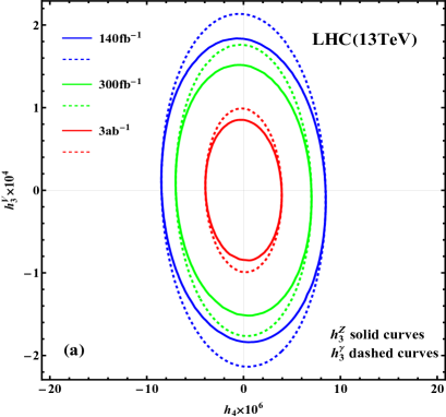
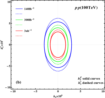
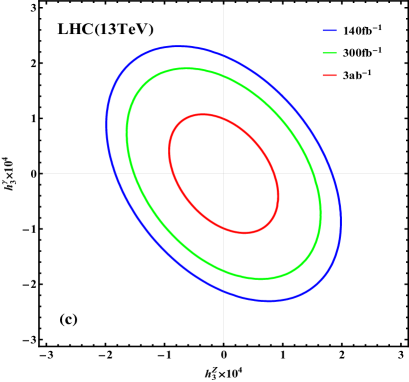
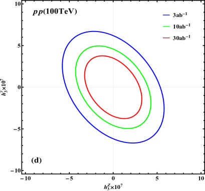
Figure 5: Correlation contours of the sensitivity reaches (95% C.L.) for the indicated pairs of nTGC form factors at the LHC (13 TeV) [ panels $(a)$ and $(c)$] and a 100 TeV $pp$ collider [ panels $(b)$ and $(d)$]. Panels (a) and (b) show the correlation contours of $(h_{4},\,h_{3}^{Z})$ (solid curves) and $(h_{4},\,h_{3}^{\gamma})$ (dashed curves), and panels (c) and (d) depict the correlation contours of $(h_{3}^{Z},\,h_{3}^{\gamma})$. 

We present our findings in Fig. 5. Panels (a) and (b) show the correlation contours of the form factors $(h_{4},\,h_{3}^{Z})$ (solid curve) and $(h_{4},\,h_{3}^{\gamma})$ (dashed curve) at the 95% C.L., and panels (c) and (d) depict the correlation contours of the form factors $(h_{3}^{Z},\,h_{3}^{\gamma})$ at the 95% C.L. Panels (a) and (c) show the correlation contours for the LHC with different integrated luminosities $\mathcal{L}=(140,\hskip 0.85358pt300,\hskip 0.85358pt3000)\hskip 0.85358pt$fb^-1 (marked by the blue, green, and red colors, respectively), and panels (b) and (d) depict the correlation contours for the 100 TeV $pp$ collider with different integrated luminosities $\mathcal{L}=(3,\hskip 0.85358pt10,\hskip 0.85358pt30)\hskip 0.85358pt$ab^-1 (marked by the blue, green, and red colors, respectively).

Inspecting Figs.5(a) and (b), we see that each elliptical contour has its axes nearly aligned with the frame axes, which shows that the form factors $(h_{4},\hskip 0.85358pth_{3}^{V})$ have rather weak correlation. This feature can be understood by examining the structure of the $\chi^{2}$ function (4.21). For a qualitative understanding of such correlation features, here we simplify Eq.(4.21) by considering a single bin analysis. Since the squared term $\sigma_{2}$ in Eq.(4.17b) dominates over the interference term $\sigma_{1}$, from Eq.(4.21) we have $\hskip 0.85358pt\chi^{2}\!\sim\\!\propto\!(\sigma_{2})^{2}\hskip 0.85358pt$, where the SM cross section $\hskip 0.85358pt\sigma_{0}\hskip 0.85358pt$ does not contain any new physics parameter and is thus irrelevant to the correlation issue. Since each elliptical contour has a fixed value of $\chi^{2}$, the cross section $\hskip 0.85358pt\sigma_{2}\hskip 0.85358pt$ is given by $\hskip 0.85358pt\sigma_{2}\!\sim\!\sqrt{\chi^{2}\hskip 0.85358pt\sigma_{0}/(\mathcal{L}\times\!\epsilon)\,}\hskip 0.85358pt$. We note that $\hskip 0.85358pt\sigma_{2}\hskip 0.85358pt$ is a quadratic function of the form factors, so we can use the usual statistical method [33][31] to analyze the quadratic function of $\hskip 0.85358pt\sigma_{2}\hskip 0.85358pt$, which suffices for examining the correlation property of each elliptical contour.

Using Eqs.(4.16) and (4.17b), we express the quadratic form of $\hskip 0.85358pt\sigma_{2}\hskip 0.85358pt$ as follows, exhibiting explicitly the energy-scaling behavior of each term:

$$\sigma_{2}\,=\,\bar{s}^{3}\hskip 0.85358pt\bar{\sigma}_{2}^{44}\hskip 0.85358pt(h_{4})^{2}+\bar{s}^{2}\hskip 0.85358pt\bar{\sigma}_{2V}^{33}\hskip 0.85358pt(h_{3}^{V})^{2}+\bar{s}^{2}\hskip 0.85358pt\bar{\sigma}_{2V}^{43}\hskip 0.85358pt(h_{4}h_{3}^{V})+\bar{s}^{2}\hskip 0.85358pt\bar{\sigma}_{2ZA}^{33}\hskip 0.85358pt(h_{3}^{Z}h_{3}^{\gamma})\,,$$ (4.22)

where $\,\bar{s}=\hat{s}/M_{Z}^{2}\,$ is a scaled dimensionless energy factor and $\hskip 0.85358pt\bar{\sigma}_{2}^{ij}\hskip 0.85358pt$ denotes the coefficient of each leading cross-section term in Eq.(4.16) in the high-energy expansion.

To examine the correlations between $h_{3}^{V}$ and $h_{4}$, only the first three terms of Eq.(4.22) are relevant. Denoting the form factors $\hskip 0.85358pt(h_{3}^{V},\hskip 0.85358pth_{4})=(x,\hskip 0.85358pty)\equiv\mathbb{X}\hskip 0.85358pt$, we can express the relevant terms of Eq.(4.22) in the following quadratic form:

$$\sigma_{2}(x,\hskip 0.85358pty) \hskip 0.85358pt=\hskip 0.85358ptA\hskip 0.85358ptx^{2}\!+B\hskip 0.85358pty^{2}\!+2\hskip 0.85358ptC\hskip 0.85358ptx\hskip 0.85358pty\,=\,\mathbb{X}\hskip 0.85358ptV^{-1}\hskip 0.85358pt\mathbb{X}^{T},$$ (4.23a)

$$V^{-1} \hskip 0.85358pt=\left(\!\!\begin{array}[]{cc}A&C\\[0.85358pt] C&B\end{array}\!\right)\!,$$ (4.23d)

where the coefficients $\,(A,\hskip 0.85358ptB,\hskip 0.85358ptC)\!\equiv\!(\bar{s}^{2}\hskip 0.85358pt\bar{\sigma}_{2V}^{33},\hskip 0.85358pt\bar{s}^{3}\hskip 0.85358pt\bar{\sigma}_{2}^{44},\hskip 0.85358pt\mbox{$\frac{\,{1}\,}{2}$}\bar{s}^{2}\hskip 0.85358pt\bar{\sigma}_{2V}^{43})\hskip 0.85358pt$. The correlation contour of $(x,\hskip 0.85358pty)$ is clearly an elliptical curve. For the above quadratic form $\,\sigma_{2}(x,\hskip 0.85358pty)\!=\!\mathbb{X}\hskip 0.85358ptV^{-1}\hskip 0.85358pt\mathbb{X}^{T}$ with two parameters $\hskip 0.85358pt\mathbb{X}\!=\!(x,\hskip 0.85358pty)\hskip 0.85358pt$, we express the covariance matrix as follows [33]:

$$V=\left(\!\begin{array}[]{cc}\hat{\sigma}_{\!x}^{2}&{\rho}\hskip 1.42262pt\hat{\sigma}_{\!x}\hskip 0.85358pt\hat{\sigma}_{\!y}\\[2.84526pt] {\rho}\hskip 1.42262pt\hat{\sigma}_{\!x}\hskip 0.85358pt\hat{\sigma}_{\!y}&\hat{\sigma}_{\!y}^{2}\end{array}\!\!\right)\!,$$ (4.26)

where $(\hat{\sigma}_{\!x},\hskip 0.85358pt\hat{\sigma}_{\!y})$ are related to the errors in the parameters $(x,\hskip 0.85358pty)$. The inverse of the covariance matrix $V$ is derived as

$$V^{-1}=\left(\!\!\!\begin{array}[]{cc}\displaystyle\frac{1}{\leavevmode\nobreak\ (1\!-\rho^{2})\hskip 0.85358pt\hat{\sigma}_{\!x}^{2}\leavevmode\nobreak\ }&\displaystyle-\frac{\rho}{\leavevmode\nobreak\ (1\!-\rho^{2})\hskip 0.85358pt\hat{\sigma}_{\!x}\hskip 0.85358pt\hat{\sigma}_{\!y}\leavevmode\nobreak\ }\\[11.38109pt] \displaystyle-\frac{\rho}{\leavevmode\nobreak\ (1\!-\rho^{2})\hskip 0.85358pt\hat{\sigma}_{\!x}\hskip 0.85358pt\hat{\sigma}_{\!y}\leavevmode\nobreak\ }&\displaystyle\frac{1}{\leavevmode\nobreak\ (1\!-\rho^{2})\hskip 0.85358pt\hat{\sigma}_{\!y}^{2}\leavevmode\nobreak\ }\end{array}\!\!\!\right)=\left(\!\!\begin{array}[]{cc}A&C\\[4.2679pt] C&B\end{array}\!\right)\!,$$ (4.31)

with the correlation parameter $\,\rho\,$ given by

$$\rho\,=\,-\hskip 0.85358ptC/\sqrt{AB\,}\,,$$ (4.32)

where $(\hat{\sigma}_{\!x},\hskip 0.85358pt\hat{\sigma}_{\!y})$ are connected to $(A,B,C)\hskip 0.85358pt$ through the relations, $\hat{\sigma}_{\!x}\!=\![(1\!-\!\rho^{2})A\hskip 0.85358pt]^{-\frac{1}{2}}\hskip 0.85358pt$ and $\hat{\sigma}_{\!y}\!=\![(1\!-\!\rho^{2})B\hskip 0.85358pt]^{-\frac{1}{2}}\hskip 0.85358pt$. Thus, using Eq.(4.23) we compute the correlation parameter (4.32) for the $(h_{3}^{V},\hskip 0.85358pth_{4})$ contour as follows:

$$\rho(h_{3}^{V},h_{4})\,=\,-\frac{\bar{\sigma}_{2V}^{43}}{\leavevmode\nobreak\ 2\sqrt{\bar{\sigma}_{2V}^{33}\hskip 0.85358pt\bar{\sigma}_{2}^{44}\,}\leavevmode\nobreak\ }\,\bar{s}^{-\frac{1}{2}}\hskip 0.85358pt.$$ (4.33)

In the above, $(\bar{\sigma}_{2}^{44},\hskip 0.85358pt\bar{\sigma}_{2V}^{33},\hskip 0.85358pt\bar{\sigma}_{2V}^{43})$ correspond to the leading-energy terms of the cross sections (4.16b)-(4.16f). We see from Eqs.(4.16b)-(4.16d) and Eqs.(4.16e)-(4.16f) that the cross section coefficients $(\bar{\sigma}_{2}^{44},\hskip 0.85358pt\bar{\sigma}_{2V}^{33})$ of the leading energy terms are always positive and the cross section coefficients $\,\bar{\sigma}_{2V}^{43}\,$ of the leading energy terms are positive for any quark flavor. Hence, we deduce that the correlation parameter $\hskip 1.42262pt\rho(h_{3}^{V},h_{4})\!<\!0\,$ in Eq.(4.33), but it is suppressed by a large energy factor $\hskip 0.85358pt1/\!\sqrt{\bar{s}\,}\,$. This means that the apex of the contour (where the slope $\hskip 0.85358pty^{\prime}\!=0\hskip 0.85358pt$) must lie on the left-hand side (LHS) of the $y$ axis. These features explain why the orientations of the contours in Figs.5(a) and (b) are not only nearly vertical, but also are aligned slightly towards the upper-left direction. Moreover, the deviation of the orientation of each contour from the vertical axis of Fig.5(b) is almost invisible because of the more severe suppression by the energy factor $\hskip 0.85358pt1/\!\sqrt{\bar{s}\,}\,$ at the 100 TeV $pp$ collider than at the LHC.

Then, we use Eq.(4.21) to perform the exact $\chi^{2}$ analysis for the form factors $(h_{3}^{Z},\hskip 0.85358pth_{3}^{\gamma})$. The $(h_{3}^{Z},\hskip 0.85358pth_{3}^{\gamma})$ contours are plotted in Figs.5(c) and (d) for the LHC and the 100 TeV $pp$ collider respectively, which show strong correlations and are oriented towards the upper-left quadrant, very different from the contours in Figs. 5(a) and (b). To understand the correlation features of Figs.5(c) and (d), we examine the relevant leading energy terms in the cross section (4.22) that include the form factors $(h_{3}^{Z},\hskip 0.85358pth_{3}^{\gamma})$ and their products. From Eq.(4.22), we find that the cross section $\hskip 0.85358pt\sigma_{2}\hskip 0.85358pt$ contains the following leading energy-dependent contributions:

$$\sigma_{2}(h_{3}^{Z},h_{3}^{\gamma}) \,=\,\bar{s}^{2}\hskip 0.85358pt\bar{\sigma}_{2Z}^{33}\hskip 0.85358pt(h_{3}^{Z})^{2}+\bar{s}^{2}\hskip 0.85358pt\bar{\sigma}_{2A}^{33}\hskip 0.85358pt(h_{3}^{\gamma})^{2}+\bar{s}^{2}\hskip 0.85358pt\bar{\sigma}_{2ZA}^{33}\hskip 0.85358pt(h_{3}^{Z}h_{3}^{\gamma})$$

$$\,=\,A\hskip 0.85358ptx^{2}+B\hskip 0.85358pty^{2}+2\hskip 0.85358ptC\hskip 0.85358ptx\hskip 0.85358pty\,=\,\mathbb{X}\hskip 0.85358ptV^{-1}\hskip 0.85358pt\mathbb{X}^{T}\,,$$ (4.34a)

$$(A,\hskip 0.85358ptB,\hskip 0.85358ptC) \,\equiv\,(\bar{s}^{2}\hskip 0.85358pt\bar{\sigma}_{2Z}^{33},\hskip 0.85358pt\bar{s}^{2}\hskip 0.85358pt\bar{\sigma}_{2A}^{33},\hskip 0.85358pt\mbox{$\frac{\,{1}\,}{2}$}\bar{s}^{2}\hskip 0.85358pt\bar{\sigma}_{2ZA}^{33})\hskip 0.85358pt,$$ (4.34b)

where we denote the form factors $\hskip 0.85358pt(h_{3}^{Z},\hskip 0.85358pth_{3}^{\gamma})\!\equiv\!(x,\hskip 0.85358pty)\!\equiv\!\mathbb{X}\,$ and the matrix $V^{-1}$ takes the form of Eq.(4.23d). Thus, using $\hskip 0.85358pt\sigma_{2}\hskip 0.85358pt$ formula in Eq.(4.34), we compute the correlation parameter (4.32) for the $(h_{3}^{Z},\hskip 0.85358pth_{3}^{\gamma})$ contour as follows:

$$\rho(h_{3}^{Z},h_{3}^{\gamma})\hskip 0.85358pt=\hskip 0.85358pt-\frac{\bar{\sigma}_{2ZA}^{33}}{\leavevmode\nobreak\ 2\sqrt{\bar{\sigma}_{2Z}^{33}\hskip 0.85358pt\bar{\sigma}_{2A}^{33}\,}\leavevmode\nobreak\ }\hskip 0.85358pt\bar{s}^{0}\hskip 0.85358pt.$$ (4.35)

This shows that the correlation parameter $\hskip 0.85358pt\rho\hskip 0.85358pt$ is of $O(\bar{s}^{0})$ and not suppressed by any energy factor, unlike the case of Eq.(4.33) which is suppressed by $\hskip 0.85358pt1/\!\sqrt{\bar{s}\,}\,$. From Eqs.(4.16c)-(4.16d) and Eq.(4.16g), we deduce that $\hskip 0.85358pt\bar{\sigma}_{2Z}^{33}\hskip 0.85358pt\bar{\sigma}_{2A}^{33}\!>\!0\hskip 0.85358pt$ and $\hskip 0.85358pt\bar{\sigma}_{2ZA}^{33}\!>\!0\hskip 0.85358pt$ always holds which lead to $\hskip 0.85358pt\rho(h_{3}^{Z},h_{3}^{\gamma})\!<\!0\hskip 0.85358pt$. These facts explain why the correlation between $\hskip 0.85358pt(h_{3}^{Z},\hskip 0.85358pth_{3}^{\gamma})\hskip 0.85358pt$ is large and all the contours of Figs. 5(c) and (d) are oriented towards the upper-left quadrant.

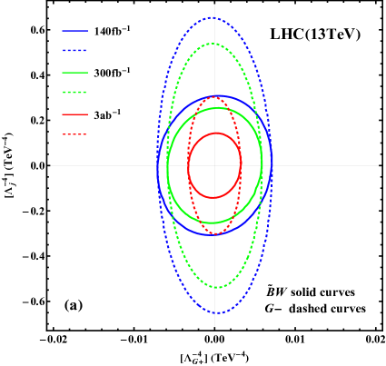
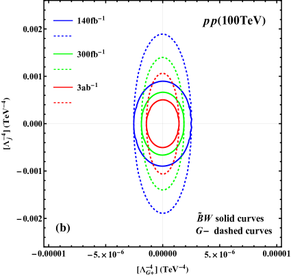
Figure 6: Correlation contours of the sensitivity reaches (95% C.L.) for the indicated pairs of nTGC operators at the LHC (13 TeV) [ panel $(a)$] and a 100 TeV $pp$ collider [ panel $(b)$]. Panels (a) and (b) show the correlation contours of $(\mathcal{O}_{G+},\,\mathcal{O}_{\widetilde{B}W})$ (solid curves) and $(\mathcal{O}_{G+},\,\mathcal{O}_{G-})$ (dashed curves). 

We then consider the nTGC formulation using the dimension-8 SMEFT operators as given in Section 2 and study correlations of the sensitivity reaches between each pair of the nTGC operators. We first study the correlations between the pairs of nTGC operators $(\mathcal{O}_{G+},\hskip 0.85358pt\mathcal{O}_{\widetilde{B}W})$ and $(\mathcal{O}_{G+},\hskip 0.85358pt\mathcal{O}_{G-})$. We perform the $\chi^{2}$ analysis using Eq.(4.21) and present the findings in Fig. 6 for the LHC (13 TeV) [panel (a)] and the 100 TeV $pp$ collider [panel (b)] for a set of sample integrated luminosities, respectively. In each panel, the $(\mathcal{O}_{G+},\hskip 0.85358pt\mathcal{O}_{\widetilde{B}W})$ correlations are shown by the contours in solid curves, whereas the $(\mathcal{O}_{G+},\hskip 0.85358pt\mathcal{O}_{G-})$ correlations are depicted by the contours in dashed curves. We see that the correlations of the operators $(\mathcal{O}_{G+},\hskip 0.85358pt\mathcal{O}_{\widetilde{B}W})$ and $(\mathcal{O}_{G+},\hskip 0.85358pt\mathcal{O}_{G-})$ are rather weak, similar to the case of the $(h_{4},\hskip 0.85358pth_{3}^{V})$ contours in Figs. 5(a) and (b).

The correlation features of the contours in Fig. 6 can be understood in the following way. Using the relations in Eq.(3.6), we here denote $\hskip 0.85358pt(x,\hskip 0.85358pty)\!=\!(h_{4},\hskip 0.85358pth_{3}^{V})\!=\!(r_{4}\bar{x},\hskip 0.85358ptr_{3}^{V}\bar{y})\hskip 0.85358pt$ and $\hskip 0.85358pt(\bar{x},\hskip 0.85358pt\bar{y})=([\Lambda_{V}^{-4}],\hskip 0.85358pt[\Lambda_{G+}^{-4}])$, where $V\!=\!Z,A$ and $(\Lambda_{Z}^{-4},\hskip 0.85358pt\Lambda_{A}^{-4})\!\equiv\!(\Lambda_{\widetilde{B}W}^{-4},\hskip 0.85358pt\Lambda_{G-}^{-4})\hskip 0.85358pt$. With these, we express the leading cross section $\hskip 0.85358pt\sigma_{2}\hskip 0.85358pt$ in Eqs.(4.22) and (4.23a) as follows:

$$\sigma_{2}(\bar{x},\hskip 0.85358pt\bar{y}) =A\hskip 0.85358pt\bar{x}^{2}+B\hskip 0.85358pt\bar{y}^{2}+2\hskip 0.85358ptC\hskip 0.85358pt\bar{x}\hskip 0.85358pt\bar{y}\,=\hskip 0.85358pt\overline{\mathbb{X}}\hskip 0.85358ptV^{-1}\hskip 0.85358pt\overline{\mathbb{X}}^{T}\hskip 0.85358pt,$$ (4.36a)

$$(A,\hskip 0.85358ptB,\hskip 0.85358ptC) \equiv\left(\bar{s}^{2}\hskip 0.85358pt(r_{3}^{V})^{2}\bar{\sigma}_{2V}^{33},\hskip 0.85358pt\bar{s}^{3}\hskip 0.85358ptr_{4}^{2}\bar{\sigma}_{2}^{44},\hskip 0.85358pt\mbox{$\frac{\,{1}\,}{2}$}\bar{s}^{2}\hskip 0.85358ptr_{3}^{V}r_{4}\bar{\sigma}_{2V}^{43}\right)\hskip 0.85358pt,$$ (4.36b)

where $\hskip 0.85358pt\overline{\mathbb{X}}\equiv(\bar{x},\hskip 0.85358pt\bar{y})\hskip 0.85358pt$ and the matrix $V^{-1}$ takes the form in Eq.(4.23d). Thus, using Eq.(4.36), we compute the correlation parameter (4.32) for $(\bar{x},\hskip 0.85358pt\bar{y})=\left([\Lambda_{V}^{-4}],\hskip 0.85358pt[\Lambda_{G+}^{-4}]\right)$ as follows:

$$\rho\!\left([\Lambda_{V}^{-4}],[\Lambda_{G+}^{-4}]\right)\,=\,-\text{sign}(r_{3}^{V}r_{4})\frac{\bar{\sigma}_{2V}^{43}\,\bar{s}^{-\frac{1}{2}}}{\leavevmode\nobreak\ 2\sqrt{\bar{\sigma}_{2V}^{33}\hskip 0.85358pt\bar{\sigma}_{2}^{44}\,}\leavevmode\nobreak\ }\,=\,\text{sign}(r_{3}^{V}r_{4})\hskip 0.85358pt\rho(h_{3}^{V},h_{4})\hskip 0.85358pt,$$ (4.37)

where the correlation parameter $\hskip 0.85358pt\rho(h_{3}^{V},h_{4})\!<\!0\,$ is derived in Eq.(4.33). According to Eq.(3.7b), we have $\hskip 0.85358pt\text{sign}(r_{3}^{Z}r_{4})\!<\!0\hskip 0.85358pt$ and $\hskip 0.85358pt\text{sign}(r_{3}^{\gamma}r_{4})\!>\!0\hskip 0.85358pt$. Thus, we can infer the signs of the corresponding correlation parameters:

$$\rho\big{(}[\Lambda_{\widetilde{B}W}^{-4}],[\Lambda_{G+}^{-4}]\big{)}>0\,,\hskip 14.22636pt\rho\!\left([\Lambda_{G-}^{-4}],[\Lambda_{G+}^{-4}]\right)<0\,.$$ (4.38)

These nicely explain why in Fig. 6 the orientations of the correlation contours (solid curves) of the operators $(\mathcal{O}_{G+},\,\mathcal{O}_{\widetilde{B}W})$ are slightly aligned towards to the right-hand-side of the vertical axis, whereas the orientations of the correlation contours (dashed curves) of the operators $(\mathcal{O}_{G+},\,\mathcal{O}_{G-})$ are slightly aligned towards to the left-hand-side of the vertical axis. Their deviations from the vertical axis are rather small because of the energy suppression factor $\hskip 0.85358pt1/\!\sqrt{\bar{s}\,}\,$ in Eq.(4.37), and they become even smaller for the contours of Fig. 6(b) at a 100 TeV $pp$ collider, as expected.

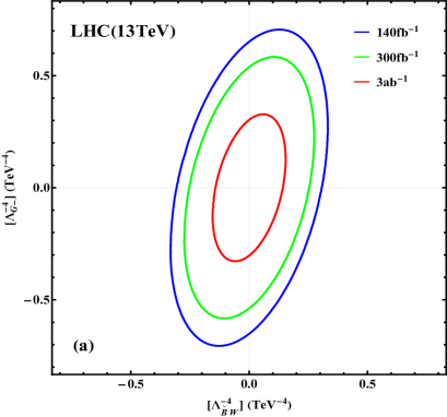
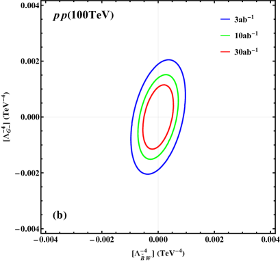
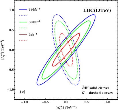
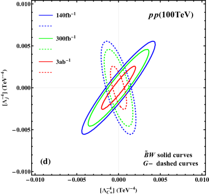
Figure 7: Correlation contours of sensitivity reaches (95% C.L.) for the indicated pairs of nTGC operators at the LHC (13 TeV) [ panels $(a)$ and $(c)$] and the 100 TeV $pp$ collider [ panels $(b)$ and $(d)$]. Panels (a) and (b) show the correlation contours of $(\mathcal{O}_{\widetilde{B}W},\,\mathcal{O}_{G-})$, whereas panels (c) and (d) depict the correlation contours of $(\mathcal{O}_{C+},\,\mathcal{O}_{\widetilde{B}W})$ (solid curves) and $(\mathcal{O}_{C+},\,\mathcal{O}_{G-})$ (dashed curves).

Next, we study the correlations between the nTGC operators $(\mathcal{O}_{\widetilde{B}W},\hskip 0.85358pt\mathcal{O}_{G-})$ and $(\mathcal{O}_{C+},\,\mathcal{O}_{G-})$. We perform a $\chi^{2}$ analysis using Eq.(4.21) and present the findings in Fig. 7. Using the relations (3.6b)-(3.6c) we find $\hskip 0.85358pt[\Lambda^{-4}_{\widetilde{B}W}]\!\propto\!h_{3}^{Z}\hskip 0.85358pt$ and $\hskip 0.85358pt[\Lambda^{-4}_{G-}]\!\propto\!h_{3}^{\gamma}\hskip 0.85358pt$. So we expect that the $(\mathcal{O}_{\widetilde{B}W},\hskip 0.85358pt\mathcal{O}_{G-})$ contour should be related to the $(h_{3}^{Z},\hskip 0.85358pth_{3}^{\gamma})$ contour. Inspecting the contours in Figs. 5(c)-(d) and Figs. 7(a)-(b), we see that they all exhibit significant correlations, but in Figs. 7(a)-(b) the contours are aligned along different directions from those of Figs. 5(c)-(d). We can understand this difference in the following way. For convenience, we define $\hskip 0.85358pt(x,\hskip 0.85358pty)\!=\!(r_{3}^{Z}\tilde{x},\hskip 0.85358ptr_{3}^{\gamma}\hskip 0.85358pt\tilde{y})\hskip 0.85358pt$ with $\widetilde{X}\equiv(\tilde{x},\hskip 0.85358pt\tilde{y})=([\Lambda^{-4}_{\widetilde{B}W}],\hskip 0.85358pt[\Lambda^{-4}_{G-}])$. With these and using Eq.(4.34), we express the leading terms of the cross section $\hskip 0.85358pt\sigma_{2}\hskip 0.85358pt$ as follows:

$$\sigma_{2}(\tilde{x},\hskip 0.85358pt\tilde{y}) \hskip 0.85358pt=\hskip 0.85358ptA\hskip 0.85358pt\tilde{x}^{2}\!+B\hskip 0.85358pt\tilde{y}^{2}\!+2\hskip 0.85358ptC\hskip 0.85358pt\tilde{x}\hskip 0.85358pt\tilde{y}\hskip 0.85358pt=\hskip 0.85358pt\widetilde{X}\hskip 0.85358ptV^{-1}\widetilde{X}^{T},$$ (4.39a)

$$(A,\hskip 0.85358ptB,\hskip 0.85358ptC) \hskip 0.85358pt=\hskip 0.85358pt\left(\bar{s}^{2}(r_{3}^{Z})^{2}\hskip 0.85358pt\bar{\sigma}_{2Z}^{33},\,\bar{s}^{2}(r_{3}^{\gamma})^{2}\hskip 0.85358pt\bar{\sigma}_{2A}^{33},\,\mbox{$\frac{\,{1}\,}{2}$}\bar{s}^{2}r_{3}^{Z}r_{3}^{\gamma}\hskip 0.85358pt\bar{\sigma}_{2ZA}^{33}\right)\!,$$ (4.39b)

where the matrix $V^{-1}$ takes the form of Eq.(4.23d).  From the above, we compute the correlation parameter (4.32) for the operators $(\mathcal{O}_{\widetilde{B}W},\hskip 0.85358pt\mathcal{O}_{G-})$ as follows:

$$\rho\big{(}[\Lambda^{-4}_{\widetilde{B}W}],[\Lambda^{-4}_{G-}]\big{)}\hskip 0.85358pt=\hskip 0.85358pt-\text{sign}(r_{3}^{Z}r_{3}^{\gamma})\hskip 0.85358pt\frac{\bar{\sigma}_{2ZA}^{33}\hskip 0.85358pt\bar{s}^{0}}{\leavevmode\nobreak\ 2\sqrt{\bar{\sigma}_{2Z}^{33}\hskip 0.85358pt\bar{\sigma}_{2A}^{33}\,}\leavevmode\nobreak\ }=\,\text{sign}(r_{3}^{Z}r_{3}^{\gamma})\hskip 0.85358pt\rho(h_{3}^{Z},h_{3}^{\gamma})\hskip 0.85358pt.$$ (4.40)

Because Eq.(3.7b) gives $\hskip 0.85358pt\text{sign}(r_{3}^{Z}r_{3}^{\gamma})\!<\!0\hskip 0.85358pt$, we deduce $\hskip 0.85358pt\rho\big{(}[\Lambda^{-4}_{\widetilde{B}W}],[\Lambda^{-4}_{G-}]\big{)}\!=\!-\rho(h_{3}^{Z},h_{3}^{\gamma})\!=\!O(\bar{s}^{0})\!\!>\!0\hskip 1.42262pt$. This explains why the contours of $\hskip 0.85358pt(\mathcal{O}_{\widetilde{B}W},\hskip 0.85358pt\mathcal{O}_{G-})\hskip 0.85358pt$ in Figs. 7(a) and (b) exhibit strong correlations [similar to those in Figs. 5(c) and (d)], but have their orientations aligned towards the upper-right quadrant [unlike Figs. 5(c) and (d), in which all the contours are oriented towards the upper-left quadrant].

Finally, we examine the correlations of the fermionic contact operator $\mathcal{O}_{C+}$ with the nTGC operators $\mathcal{O}_{\widetilde{B}W}$ and $\mathcal{O}_{G-}$. Since $\mathcal{O}_{C+}$ is a combination of two other operators $\hskip 0.85358pt\mathcal{O}_{C+}\!\!=\mathcal{O}_{G-}\!-\mathcal{O}_{\widetilde{B}W}\hskip 0.85358pt$ viathe equation of motions (2.3a), it is connected to both of the form factors $(h_{3}^{Z},\hskip 0.85358pth_{3}^{\gamma})$, which would complicate the correlation analysis in the form factor formulation (4.16). Instead, we analyze directly the contributions of the operators $(\mathcal{O}_{C+},\hskip 0.85358pt\mathcal{O}_{G-},\hskip 0.85358pt\mathcal{O}_{\widetilde{B}W})$ to the helicity amplitudes (2.8)-(2.9). As shown by Eq.(2.9), the operator $\mathcal{O}_{C+}$ has a nonzero left-handed coupling $\hskip 0.85358ptc_{L(C+)}^{\prime}\!\!=\!-T_{3}\hskip 1.42262pt$ only. So for examining its correlations with $\mathcal{O}_{G-}$ and $\mathcal{O}_{\widetilde{B}W}$, the contributions of $\mathcal{O}_{G-}$ and $\mathcal{O}_{\widetilde{B}W}$ from the left-handed-quark couplings $\hskip 0.85358ptc_{L(G-)}^{\prime}\hskip 0.85358pt$ and $\hskip 0.85358ptc_{L(\widetilde{B}W)}^{\prime}\hskip 0.85358pt$ play key roles. Thus, we can express as follows the relevant helicity amplitudes (2.8)-(2.9) containing left-handed (right-handed) initial-state quarks:

$$\mathcal{T}_{8L} \,=\,\overline{\mathcal{T}}_{\!8L}\!\times\!\big{\{}c_{L(C+)}^{\prime}[\Lambda_{C+}^{-4}]+c_{L(\!\widetilde{B}W)}^{\prime}[\Lambda_{\widetilde{B}W}^{-4}]+c_{L(G-)}^{\prime}[\Lambda_{G-}^{-4}]\big{\}}$$

$$\,=\,\overline{\mathcal{T}}_{\!8L}\hskip 0.85358pt(f_{L0}\hskip 0.85358ptx+f_{L1}\hskip 0.85358pty_{1}+f_{L2}\hskip 0.85358pty_{2})\,,$$ (4.41a)

$$\mathcal{T}_{8R} \,=\,\overline{\mathcal{T}}_{\!8R}\!\times\!\big{\{}c_{R(\!\widetilde{B}W)}^{\prime}[\Lambda_{\widetilde{B}W}^{-4}]+c_{R(G-)}^{\prime}[\Lambda_{G-}^{-4}]\big{\}}\hskip 0.85358pt\equiv\hskip 0.85358pt\overline{\mathcal{T}}_{\!8R}\,(f_{R1}\hskip 0.85358pty_{1}\!+\!f_{R2}\hskip 0.85358pty_{2})\,,$$ (4.41b)

where $\overline{\mathcal{T}}_{8L}$ (or $\overline{\mathcal{T}}_{8R}$) is the remaining common part of the helicity amplitudes (2.8)-(2.9) after separating out the coupling $\hskip 0.85358ptc_{Lj}^{\prime}$ (or $\hskip 0.85358ptc_{Rj}^{\prime}$) and the cutoff factor $[\Lambda_{j}^{-4}]$. In the above, we have defined $\hskip 0.85358pt(x,\hskip 0.85358pty_{1},\hskip 0.85358pty_{2})\!\equiv\!([\Lambda_{C+}^{-4}],\hskip 0.85358pt[\Lambda_{\widetilde{B}W}^{-4}],\hskip 0.85358pt[\Lambda_{G-}^{-4}])\hskip 0.85358pt$ and

$$f_{L0} =c_{L(C+)}^{\prime}\!=-T_{3}\hskip 0.85358pt,\leavevmode\nobreak\ \leavevmode\nobreak\ \leavevmode\nobreak\ f_{L1}\!=c_{\!L(\widetilde{B}W)}^{\prime}\!=T_{3}\!-Qs_{W}^{2}\hskip 0.85358pt,\leavevmode\nobreak\ \leavevmode\nobreak\ \leavevmode\nobreak\ f_{L2}\!=c_{L(G-)}^{\prime}\!=-Qs_{W}^{2}\hskip 0.85358pt,$$ (4.42a)

$$f_{R1} =c_{\!R(\widetilde{B}W)}^{\prime}\!=-Qs_{W}^{2}\hskip 0.85358pt,\leavevmode\nobreak\ \leavevmode\nobreak\ \leavevmode\nobreak\ f_{R2}=c_{R(G-)}^{\prime}\!=c_{L(G-)}^{\prime}\!=f_{L2}\equiv f_{2}\,.$$ (4.42b)

With the above, we perform a $\chi^{2}$ analysis based upon Eq.(4.21). We present the correlation contours of $(\mathcal{O}_{C+},\hskip 0.85358pt\mathcal{O}_{\widetilde{B}W})$ and $(\mathcal{O}_{C+},\hskip 0.85358pt\mathcal{O}_{G-})$ in Figs. 7(c) and (d) for the LHC and the 100 TeV $pp$ collider, respectively. We find that all these contours exhibit strong correlations. In particular, the $(\mathcal{O}_{C+},\hskip 0.85358pt\mathcal{O}_{\widetilde{B}W})$ contours (solid curves) are oriented towards the upper-right quadrant, whereas the $(\mathcal{O}_{C+},\hskip 0.85358pt\mathcal{O}_{G-})$ contours (dashed curves) are oriented towards the upper-left quadrant.

To understand the qualitative features of the correlation contours in Figs. 7(c) and (d), we examine the cross section $\sigma_{2}$, which contains the squared part of the dimension-8 contributions and dominates the $\chi^{2}$ function. From Eq.(4.41), we derive the cross section $\sigma_{2}$ as follows:

$$\sigma_{2}(x,y_{1},y_{2}) \,=\,(f_{L0}\hskip 0.85358ptx+\!f_{L1}\hskip 0.85358pty_{1}\!+\!f_{2}\hskip 0.85358pty_{2})^{2}\!\left<|\overline{\mathcal{T}}_{\!8L}|^{\,2}\right>+(f_{R1}\hskip 0.85358pty_{1}\!+\!f_{2}\hskip 0.85358pty_{2})^{2}\!\left<|\overline{\mathcal{T}}_{\!8R}|^{\,2}\right>$$

$$\,=\,\left[(f_{L0}\hskip 0.85358ptx+\!f_{L1}\hskip 0.85358pty_{1}\!+\!f_{2}\hskip 0.85358pty_{2})^{2}\!+\!(f_{R1}\hskip 0.85358pty_{1}\!+\!f_{2}\hskip 0.85358pty_{2})^{2}\right]\!\left<|\overline{\mathcal{T}}_{\!8}|^{\,2}\right>,$$ (4.43)

where we have defined the notations $\left<|\overline{\mathcal{T}}_{\!8L}|^{\,2}\right>\!=\!\int_{\mathrm{PS}}|\overline{\mathcal{T}}_{\!8L}|^{\,2}$ and $\left<|\overline{\mathcal{T}}_{\!8R}|^{\,2}\right>\!=\!\int_{\mathrm{PS}}|\overline{\mathcal{T}}_{\!8R}|^{\,2}$ with $\int_{\mathrm{PS}}$ denoting the phase space integration for the final state. From the squared term of the cross section (2.2), we can further deduce the equality $\left<|\overline{\mathcal{T}}_{\!8L}|^{\,2}\right>\!=\!\left<|\overline{\mathcal{T}}_{\!8R}|^{\,2}\right>\!\equiv\!\left<|\overline{\mathcal{T}}_{\!8}|^{\,2}\right>$, which is used in the last step of Eq.(4.43).

For analyzing the correlations, the overall factor $\left<|\overline{\mathcal{T}}_{\!8}|^{\,2}\right>$ is irrelevant. So we define the following rescaled cross sections for the convenience of analyzing the two-parameter correlations:

$$\bar{\sigma}_{2}(x,y_{1})\equiv\sigma_{2}(x,y_{1},0)/\!\left<|\overline{\mathcal{T}}_{\!8}|^{\,2}\right>,\leavevmode\nobreak\ \leavevmode\nobreak\ \leavevmode\nobreak\ \leavevmode\nobreak\ \bar{\sigma}_{2}(x,y_{2})\equiv\sigma_{2}(x,0,y_{2})/\!\left<|\overline{\mathcal{T}}_{\!8}|^{\,2}\right>.$$ (4.44)

Thus, $\hskip 0.85358pt\bar{\sigma}_{2}(x,y_{1})\hskip 0.85358pt$ and $\hskip 0.85358pt\bar{\sigma}_{2}(x,y_{2})\hskip 0.85358pt$ are expressed in the following quadratic form:

$$\bar{\sigma}_{2}(x,y_{1}) =\,A\hskip 0.85358ptx^{2}+B_{1}y_{1}^{2}+2\hskip 0.85358ptC_{1}\hskip 0.85358ptx\hskip 0.85358pty_{1}\equiv\hskip 0.85358pt\mathbb{X}_{1}V_{1}^{-1}\hskip 0.85358pt\mathbb{X}_{1}^{T}\,,$$ (4.45a)

$$\bar{\sigma}_{2}(x,y_{2}) =\,A\hskip 0.85358ptx^{2}+B_{2}y_{2}^{2}+2\hskip 0.85358ptC_{2}\hskip 0.85358ptx\hskip 0.85358pty_{2}\equiv\hskip 0.85358pt\mathbb{X}_{2}V_{2}^{-1}\hskip 0.85358pt\mathbb{X}_{2}^{T}\,,$$ (4.45b)

where we have defined $\hskip 0.85358pt\mathbb{X}_{1}\!\equiv\!(x,\hskip 0.85358pty_{1})\hskip 0.85358pt$ and $\hskip 0.85358pt\mathbb{X}_{2}\!\equiv\!(x,\hskip 0.85358pty_{2})\hskip 0.85358pt$ as well as the following notations,

$$(A,\hskip 0.85358ptB_{1},\hskip 0.85358ptC_{1}) \equiv(f_{L0}^{2},\,f_{L1}^{2}\!+\!f_{R1}^{2},\,f_{L0}f_{L1})\hskip 0.85358pt,$$ (4.46a)

$$(A,\hskip 0.85358ptB_{2},\hskip 0.85358ptC_{2}) \equiv(f_{L0}^{2},\,2\hskip 0.85358ptf_{2}^{2},\,f_{L0}f_{2})\hskip 0.85358pt,$$ (4.46b)

$$V_{1}^{-1} =\!\left(\!\!\!\begin{array}[]{cc}A&C_{1}\\ \hskip 0.85358ptC_{1}&B_{1}\end{array}\!\!\right)\!,\leavevmode\nobreak\ \leavevmode\nobreak\ \leavevmode\nobreak\ \leavevmode\nobreak\ V_{2}^{-1}=\!\left(\!\!\!\begin{array}[]{cc}A&C_{2}\\ \hskip 0.85358ptC_{2}&B_{2}\end{array}\!\!\right)\!.$$ (4.46g)

Thus, we can deduce the following correlation parameter for the two cases:

$$\rho_{1}(x,y_{1}) \,=\hskip 0.85358pt\frac{-\hskip 0.85358ptC_{1}}{\,\sqrt{AB_{1}}\,}=\frac{\leavevmode\nobreak\ -\hskip 0.85358pt\text{sign}(f_{L0}f_{L1})\leavevmode\nobreak\ }{\,\sqrt{1\!+\!f_{R1}^{2}/\!f_{L1}^{2}\,}\,}>0\,,$$ (4.47a)

$$\rho_{2}(x,y_{2}) \,=\hskip 0.85358pt\frac{-\hskip 0.85358ptC_{2}}{\,\sqrt{AB_{2}}\,}=-\frac{1}{\sqrt{2\,}\,}\hskip 0.85358pt\text{sign}(f_{L0}f_{2})<0\,,$$ (4.47b)

where $\hskip 0.85358pt(x,\hskip 0.85358pty_{1})\equiv([\Lambda_{C+}^{-4}],\hskip 0.85358pt[\Lambda_{\widetilde{B}W}^{-4}])\hskip 0.85358pt$ and $(x,\hskip 0.85358pty_{2})\equiv([\Lambda_{C+}^{-4}],\hskip 0.85358pt[\Lambda_{G-}^{-4}])$. Using the coupling formula (4.42), we derive $\hskip 0.85358ptf_{L0}\hskip 0.85358ptf_{L1}\!=\!-T_{3}\hskip 0.85358pt(T_{3}-Qs_{W}^{2})\!<0\,$ and $\hskip 0.85358ptf_{L0}f_{2}\!=\!T_{3}Q\hskip 0.85358pts_{W}^{2}\!>0\,$, where each inequality holds for both up-type and down-type quarks. From these, we deduce that the operators $(\mathcal{O}_{C+},\hskip 0.85358pt\mathcal{O}_{\widetilde{B}W})$ are correlated positively, whereas the operators $(\mathcal{O}_{C+},\hskip 0.85358pt\mathcal{O}_{G-})$ are correlated negatively. Moreover, Eq.(4.47) shows that both correlation parameters are of $\hskip 0.85358ptO(\bar{s}^{0})\hskip 0.85358pt$ and not suppressed by any energy factor. This predicts strong correlations for the operators $(\mathcal{O}_{C+},\hskip 0.85358pt\mathcal{O}_{\widetilde{B}W})$ and $(\mathcal{O}_{C+},\hskip 0.85358pt\mathcal{O}_{G-})$, respectively. These features are indeed reflected in Figs. 7(c) and (d). We see that the correlation contours of $\,(\mathcal{O}_{C+},\,\mathcal{O}_{\widetilde{B}W})$ (solid curves) are oriented towards the upper-right quadrant due to the positive correlation parameter $\hskip 0.85358pt\rho_{1}(x,y_{1})\!>\!0\,$ given by Eq.(4.47a), whereas the correlation contours of $(\mathcal{O}_{C+},\,\mathcal{O}_{G-})$ (dashed curves) are aligned towards the upper-left quadrant due to the negative correlation parameter $\hskip 0.85358pt\rho_{2}(x,y_{2})\!<\!0\,$ given by Eq.(4.47b).

4.7 Comparison with the Existing LHC Bounds on nTGCs

In this subsection, we make direct comparison with the published LHC measurements of nTGCs through the reaction $\hskip 0.85358ptp{\hskip 0.85358pt}p{\hskip 0.85358pt}(q{\hskip 0.85358pt}\bar{q})\!\rightarrow\!Z\gamma\hskip 0.85358pt$ with $Z\!\!\rightarrow\!\nu{\hskip 0.85358pt}\bar{\nu}{\hskip 0.85358pt}\hskip 0.85358pt$ by the ATLAS [19] and CMS [18] collaborations using the conventional nTGC form factor formula (3.1). The CMS collaboration analyzed 19.6 fb^-1 of Run-1 data at $\sqrt{s\,}\!=\!8$ TeV [18], whereas the ATLAS collaboration analyzed 36.1 fb^-1 of Run-2 data at $\sqrt{s\,}=13$ TeV [19]. They obtained the following sensitivity bounds (95% C.L.) on the form factors:

CMS: $$h_{3}^{Z}\in(-1.5,\,1.6)\!\times\!10^{-3}, h_{3}^{\gamma}\in(-1.1,\,0.9)\!\times\!10^{-3},$$

$$h_{4}^{Z}\in(-3.9,\,4.5)\!\times\!10^{-6}, h_{4}^{\gamma}\in(-3.8,\,4.3)\!\times\!10^{-6};$$ (4.48a)

ATLAS: $$h_{3}^{Z}\in(-3.2,\,3.3)\!\times\!10^{-4}, h_{3}^{\gamma}\in(-3.7,\,3.7)\!\times\!10^{-4},$$

$$h_{4}^{Z}\in(-4.5,\,4.4)\!\times\!10^{-7}, h_{4}^{\gamma}\in(-4.4,\,4.3)\!\times\!10^{-7}.$$ (4.48b)

We see that the CMS and ATLAS analyses both obtained much stronger bounds on $(h_{4}^{Z},\,h_{4}^{\gamma})$ than on $(h_{3}^{Z},\,h_{3}^{\gamma})$, i.e., by factors $\sim\!(210-380)$ at CMS (Run-1) and $\sim\!(710-860)$ at ATLAS (Run-2). In comparison, we see in Table 7 using our SMEFT form factor formulation (3.5) that the LHC sensitivity bounds on $h_{4}^{V}$ are stronger than those on $\hskip 0.85358pth_{3}^{V}$ only by factors of about $20\hskip 0.85358pt$. Our Table 8 further demonstrates that using the conventional form factor formulation (3.1) would generate spuriously stronger $h_{4}^{V}$ bounds (marked in blue) at the LHC (13 TeV) than the SMEFT bounds (marked in red) by a factor of about $20$, and thus much stronger than the $h_{3}^{V}$ bounds by a large factor of $\sim\!20\!\times\!20=400\hskip 0.85358pt$, which agrees with the ATLAS results in Eq.(4.48) within a factor of $2\hskip 1.42262pt$. Unfortunately, this means that the strong experimental bounds (4.48) on $(h_{4}^{Z},\,h_{4}^{\gamma})$ are unreliable because they were obtained by using the conventional form factor formulation (3.1), which does not respect the SM electroweak gauge symmetry of SU(2)${}_{\mathrm{L}}\otimes\hskip 0.85358pt$U(1)_Y as incorporated in the SMEFT.

To study quantitatively the conventional parametrization (3.1) including the nTGC form factors $(h_{3}^{V},\hskip 0.85358pth_{4}^{V})$ only, we denote their contributions to the total cross section by $\,\widetilde{\sigma}(Z\gamma)\!=\sigma_{0}+\widetilde{\sigma}_{1}+\widetilde{\sigma}_{2}\,$, where $\widetilde{\sigma}_{1}$ is the interference term and $\widetilde{\sigma}_{2}$ is the squared contribution. This is similar to what we did around Eq.(4.18). We find that $\widetilde{\sigma}_{2}$ always dominates over $\widetilde{\sigma}_{1}$ for both the LHC and the 100 TeV $pp$ collider. Using the conventional form factor formula (3.1), we derive the squared contribution $\widetilde{\sigma}_{2}$ as follows:

$$\widetilde{\sigma}_{2}=\frac{\leavevmode\nobreak\ e^{4}(X_{LR}^{V})^{2}(\hat{s}-M_{Z}^{2})^{3}\!\left[4(h_{3}^{V})^{2}\!\left(\!\frac{M_{Z}^{2}}{\hat{s}}+1\!\right)\!+4\hskip 0.85358pth_{3}^{V}h_{4}^{V}\!\left(\!1\!-\!\frac{\hat{s}}{M_{Z}^{2}}\!\right)\!+\!(h_{4}^{V})^{2}\!\left(\!1\!-\!\frac{\hat{s}}{M_{Z}^{2}}\!\right)^{\!\!2}\right]\leavevmode\nobreak\ }{768\hskip 0.85358pt\pi\hskip 0.85358pts_{W}^{2}c_{W}^{2}M_{Z}^{6}\,\hat{s}},$$ (4.49)

where the coupling factor $(X_{LR}^{V})^{2}$ is defined as

$$(X_{LR}^{V})^{2}\equiv(X_{L}^{V})^{2}\!+\!(X_{R}^{V})^{2},\leavevmode\nobreak\ \leavevmode\nobreak\ \leavevmode\nobreak\ \leavevmode\nobreak\ X_{L,R}^{Z}\equiv x_{L,R}^{Z}\,,\leavevmode\nobreak\ \leavevmode\nobreak\ \leavevmode\nobreak\ \leavevmode\nobreak\ X_{L,R}^{\gamma}\equiv-\frac{c_{W}}{s_{W}}x_{L,R}^{A}\,,\hskip 28.45274pt$$ (4.50a)

$$(x_{L}^{Z},\hskip 0.85358ptx_{R}^{Z})=(T_{3}\!-\!Qs_{W}^{2},\hskip 0.85358pt-Qs_{W}^{2})\hskip 0.85358pt,\leavevmode\nobreak\ \leavevmode\nobreak\ \leavevmode\nobreak\ \leavevmode\nobreak\ (x_{L}^{A},\hskip 0.85358ptx_{R}^{A})=-Qs_{W}^{2}(1,\hskip 0.85358pt1)\hskip 0.85358pt.$$ (4.50b)

Defining a scaled dimensionless energy parameter $\,\bar{s}=\hat{s}/M_{Z}^{2}\,$ and making the high-energy expansion for $\,\bar{s}\!\gg\!1\,$, we can compare the leading energy-dependence of each term of $\,\widetilde{\sigma}_{2}$ with that of $\,\sigma_{2}\hskip 0.85358pt$, as follows:

$$\widetilde{\sigma}_{2} \,\approx\,\frac{\leavevmode\nobreak\ e^{4}(X_{LR}^{V})^{2}\!\left[(h_{4}^{V})^{2}\hskip 0.85358pt\bar{s}^{4}\!-4\hskip 0.85358pth_{4}^{V}h_{3}^{V}\bar{s}^{3}\!+4(h_{3}^{V})^{2}\hskip 0.85358pt\bar{s}^{2}\hskip 0.85358pt\right]\leavevmode\nobreak\ }{768\hskip 0.85358pt\pi\hskip 0.85358pts_{W}^{2}\hskip 0.85358ptc_{W}^{2}M_{Z}^{2}}\hskip 0.85358pt,$$ (4.51a)

$$\sigma_{2} \,\approx\,\frac{\leavevmode\nobreak\ e^{4}\!\left[T_{3}^{2}(h_{4}^{Z})^{2}\hskip 0.85358pt\bar{s}^{3}\!+8\hskip 0.85358ptT_{3}X_{L}^{V}h_{4}^{Z}h_{3}^{V}\hskip 0.85358pt\bar{s}^{2}\!+\!4\hskip 0.85358pt(X_{LR}^{V})^{2}(h_{3}^{V})^{2}\hskip 0.85358pt\bar{s}^{2}\hskip 0.85358pt\right]\leavevmode\nobreak\ }{\leavevmode\nobreak\ 768\hskip 0.85358pt\pi s_{W}^{2}\hskip 0.85358ptc_{W}^{2}M_{Z}^{2}\,}\hskip 0.85358pt,$$ (4.51b)

where the cross section $\,\sigma_{2}\hskip 0.85358pt$ is given by our SMEFT form factor formula (3.5). We note that the form factors $(h_{4}^{Z},\,h_{4}^{\gamma})$ in the above cross section $\hskip 0.85358pt\sigma_{2}\hskip 0.85358pt$ should obey the condition (3.4b) due to the underlying electroweak gauge symmetry of the SM that is respected by the corresponding dimension-8 nTGC operators. We have used the relation (3.4b) to combine the $\hskip 0.85358pth_{4}^{\gamma}\hskip 0.85358pt$ contribution with that of $\hskip 0.85358pth_{4}^{Z}\hskip 0.85358pt$. To examine the correlation of $(h_{3}^{\gamma},\,h_{4}^{\gamma})$ from Eq.(4.51b), we can use Eq.(3.4b) to replace $\hskip 0.85358pth_{4}^{Z}\hskip 0.85358pt$ by $\hskip 0.85358pth_{4}^{\gamma}\hskip 0.85358pt$. Inspecting Eq.(4.51), we see that both the $(h_{4}^{V})^{2}$ and $(h_{4}^{V}h_{3}^{V})$ terms in $\hskip 0.85358pt\widetilde{\sigma}_{2}$ have higher energy dependences than those of $\sigma_{2}$ by an extra factor $\hskip 0.85358pt\bar{s}^{1}$, which leads erroneously to much stronger bounds on $h_{4}^{V}\hskip 0.85358pt$.

We first make a one-parameter analysis and derive the bound on each form factor coefficient $\,h_{j}^{V}$ individually (where $j\!=\!3,4\hskip 0.85358pt$ and $\hskip 0.85358ptV\!=\!Z,\gamma\,$) using the conventional form factor parametrization (3.1). To make a more precise comparison with the ATLAS bounds (4.48), we adopt the same kinematic cut on the transverse momentum of the final-state photon, $P_{T}^{\gamma}$ > 600 GeV, and the same integrated luminosity $\hskip 0.85358pt\mathcal{L}=36.1$ fb^-1 as in the ATLAS analysis [19]. For illustration, we ignore the other detector-level cuts and the systematic errors, and choose a typical detection efficiency $\,\epsilon\!=\!75\%\hskip 1.42262pt$.  With these, we derive the following bounds on the nTGCs (95% C.L.) when using the conventional form factor parametrization (3.1):

$$|h_{3}^{Z}|<3.0\!\times\!10^{-4},\hskip 14.22636pt|h_{3}^{\gamma}|<3.4\!\times\!10^{-4},\hskip 14.22636pt|h_{4}^{Z}|<4.4\!\times\!10^{-7},\hskip 14.22636pt|h_{4}^{\gamma}|<4.9\!\times\!10^{-7},$$ (4.52)

and note that the squared nTGC contributions dominate the sensitivity. Comparing the above estimated bounds (4.52) with the ATLAS experimental bounds (4.48), we see that they agree well with each other: the agreements for $h_{4}^{Z}$ are within about $2\%\hskip 1.42262pt$ and the agreements for $(h_{4}^{\gamma},h_{3}^{Z},\hskip 0.85358pth_{3}^{\gamma})$ are within about $(8\!-\!13)\%\hskip 1.42262pt$. This means that by making plausible simplifications we can reproduce quite accurately the experimental bounds (4.48) established by the ATLAS collaboration [19] using the conventional form factor formulation in Eq.(3.1).

Next, we analyze the correlation contours for $(h_{3}^{\gamma},\hskip 0.85358pth_{4}^{\gamma})$ and $(h_{3}^{Z},\hskip 0.85358pth_{4}^{Z})$, respectively, using the conventional form factor parametrization (3.1), which can be compared to the correlation contours obtained by using our SMEFT form factor formulation (3.5). Fig. 8 displays the correlation contours at 95% C.L. for LHC Run-2. Panels (a) and (b) show the correlation contours based on the SMEFT form factor formula (3.5), where the blue (red) contours correspond to inputting integrated LHC luminosities of $36.1\hskip 0.85358pt$fb^-1 ($140\hskip 0.85358pt$fb^-1). Panels (c) and (d) present the correlation contours based on the conventional form factor parametrization (3.1), where the red and blue contours are given by our theoretical analysis with the assumed detection efficiencies $\hskip 0.85358pt\epsilon\!=\!100\%\hskip 0.85358pt$ and $\hskip 0.85358pt\epsilon\!=\!75\%\hskip 0.85358pt$ respectively. For comparison, we show in panels (c) and (d) the experimental contours as extracted from the ATLAS results [19] based on the conventional form factor formula (3.1), where the black solid curves depict the observed bounds and the black dashed curves show the expected limits. It is impressive to see in panels (c) and (d) that our theoretical contours agree well with the experimental contours obtained by using the conventional form factor parametrization (3.1).

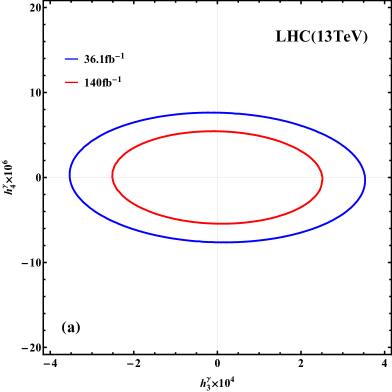
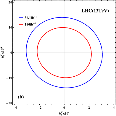
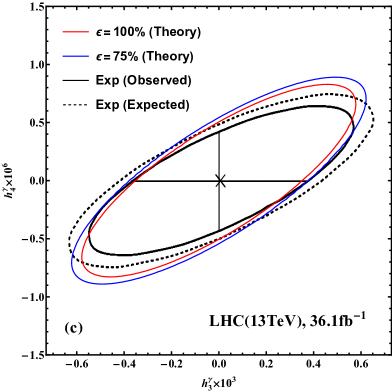
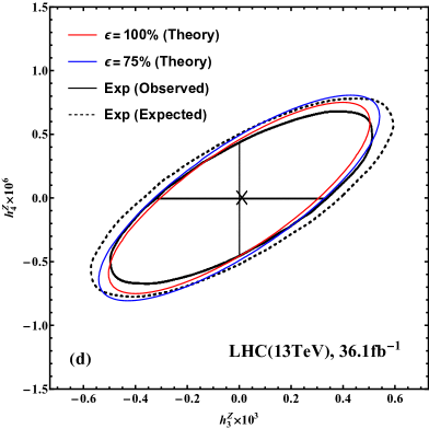
Figure 8: Correlation contours of the sensitivity reaches (95% C.L.) for the indicated pairs of nTGC form factors at the LHC (13 TeV). Panels (a) and (b) present the correlation contours for $(h_{3}^{\gamma},\,h_{4}^{\gamma})$ and $(h_{3}^{Z},\,h_{4}^{Z})$ respectively, by using our SMEFT form factor formula (3.5), where in each panel the red contour inputs the full integrated luminosity 140 fb${}^{-1}\!\!$ of Run-2 and the blue contour inputs a partial integrated luminosity 36.1 fb${}^{-1}\!$ as in the ATLAS analysis [19]. Panels (c) and (d) compare the theoretical correlation contours (red and blue colors) with the experimental contours (black color) from the ATLAS analysis [19], where we derived the red and blue contours by using the conventional form factor formula (3.1) and by assuming an ideal detection efficiency $\epsilon\!=\!100\%$ (for red contours) or a reduced detection efficiency $\hskip 0.85358pt\epsilon\!=\!75\%$ (for blue contours). The ATLAS contours are shown by the black solid curves (observed) and the black dashed curves (expected).

We note that the correlation contours of panels (a) and (b) in Fig. 8 have very different features from those of panels (c) and (d), which can be understood as follows. For convenience, we denote $\hskip 0.85358pt\mathbb{X}\!=\!(x,\,y)\!\equiv\!(h_{3}^{V},\hskip 0.85358pth_{4}^{Z})$. Thus, we can express the cross sections of Eqs.(4.51a) and (4.51b) as follows:

$$\widetilde{\sigma}_{2} \,\propto\,\widetilde{A}{x}^{2}\!+\widetilde{B}{y}^{2}\!+2\hskip 0.85358pt\widetilde{C}{x}\hskip 0.85358pt{y}\hskip 0.85358pt\equiv\hskip 0.85358pt\mathbb{X}\hskip 0.85358pt\widetilde{V}^{-1}\hskip 0.85358pt\mathbb{X}^{T},$$ (4.53a)

$$\sigma_{2} \,\propto\,Ax^{2}\!+By^{2}\!+2\hskip 0.85358ptCx\hskip 0.85358pty\hskip 0.85358pt\equiv\hskip 0.85358pt\mathbb{X}\hskip 0.85358ptV^{-1}\hskip 0.85358pt\mathbb{X}^{T},$$ (4.53b)

where we have defined the following notations,

$$(\widetilde{A},\hskip 0.85358pt\widetilde{B},\hskip 0.85358pt\widetilde{C}) \,=\hskip 0.85358pt(4\hskip 0.85358pt\bar{s}^{2},\hskip 0.85358pt\bar{s}^{4},\hskip 0.85358pt-2\bar{s}^{3})\hskip 0.85358pt,$$ (4.54a)

$$(A,\hskip 0.85358ptB,\hskip 0.85358ptC) \,=\hskip 0.85358pt\left(4\hskip 0.85358pt\bar{s}^{2}(X_{LR}^{V})^{2},\hskip 0.85358pt\bar{s}^{3}T_{3}^{2},\hskip 0.85358pt4\hskip 0.85358pt\bar{s}^{2}X_{L}^{V}T_{3}\right),$$ (4.54b)

$$\widetilde{V}^{-1} =\!\left(\!\!\!\begin{array}[]{cc}\widetilde{A}&\widetilde{C}\\[1.13809pt] \hskip 0.85358pt\widetilde{C}&\widetilde{B}\end{array}\!\right)\!,\leavevmode\nobreak\ \leavevmode\nobreak\ \leavevmode\nobreak\ \leavevmode\nobreak\ V^{-1}=\!\left(\!\!\!\begin{array}[]{cc}A&C\\[0.85358pt] \hskip 0.85358ptC&B\end{array}\!\right)\!.$$ (4.54g)

With these we can compute the correlation parameter of the form factors in each case:

$$\widetilde{\rho}\hskip 0.85358pt=\frac{-\hskip 0.85358pt\widetilde{C}}{\,\sqrt{\widetilde{A}\hskip 0.85358pt\widetilde{B}\,}\,}=1\!>0\,,\leavevmode\nobreak\ \leavevmode\nobreak\ \leavevmode\nobreak\ \leavevmode\nobreak\ \leavevmode\nobreak\ \rho\hskip 0.85358pt=\frac{-\hskip 0.85358ptC}{\,\sqrt{AB\,}\,}=-\frac{\,2\hskip 1.42262pt\text{sign}(T_{3})X_{L}^{V}\,}{|X_{LR}^{V}|\,}\hskip 0.85358pt\bar{s}^{-\frac{1}{2}}\!<0\,.$$ (4.55)

The fact of $\hskip 0.85358pt\widetilde{\rho}\!=\!O(\bar{s}^{0})\!\!>\!0\hskip 0.85358pt$ explains why the $\hskip 0.85358pt(h_{3}^{V},\hskip 0.85358pth_{4}^{V})\,$ contours in Figs. 8(c) and (d) exhibit strong correlations and have their orientations aligned towards the upper-right quadrant. On the other hand, from Eq.(4.50) we find that $\hskip 0.85358pt\text{sign}(T_{3})X_{L}^{V}\!>\!0\,$ holds for the initial-state quarks being either up-type or down-type, and thus Eq.(4.55) gives $\hskip 0.85358pt\rho\!<\!0\hskip 1.42262pt$. This means that the $\hskip 0.85358pt(h_{3}^{V},\hskip 0.85358pth_{4}^{V})\,$ contours in Figs. 8(a) and (b) should have their orientations towards the upper-left quadrant, but this correlation is almost invisible because $\hskip 0.85358pt\rho\!=\!O(\bar{s}^{-\frac{1}{2}})\hskip 0.85358pt$ receives a large energy-suppression factor at the LHC. Thus, the correlation features of the $\hskip 0.85358pt(h_{3}^{V},\hskip 0.85358pth_{4}^{V})\,$ contours are well understood both for Figs. 8(a)-(b) [based on the SMEFT form factor formula (3.5)] and for Figs. 8(c)-(d) [based on the conventional form factor formula (3.1)].

Our quantitative comparisons in Figs. 8 are instructive and encouraging. We suggest that the ATLAS and CMS colleagues perform a systematic nTGC analysis based on the new SMEFT form factor formula (3.5), using the full Run-2 data set. Moreover, we note that in Refs. [18]-[19] the CMS and ATLAS collaborations analyzed the correlations between the form factors $(h_{3}^{V},\,h_{4}^{V})$ and found strong correlations. We have reproduced this feature in Figs. 8(c)-(d), but we note that those correlation contours differ substantially from our new correlation contours in Figs. 8(a)-(b). Based upon the above analysis, we suggest that the CMS and ATLAS collaborations should make updated analyses on the $(h_{3}^{V},\,h_{4}^{V})$ correlations using our new SMEFT form factor formulation with their full Run-2 data sets.  We anticipate that such new analyses should yield results similar to the theoretical predictions for LHC Run-2 given in Table 7 and Figs. 8(a)-(b).

5 Comparison with Probes of nTGCs at Lepton Colliders

In this Section we first summarize the sensitivity reaches of nTGC new physics scales at high-energy $e^{+}e^{-}$ colliders found in our previous work [5]. Then we analyze the sensitivity reaches of the nTGC form factors at these $e^{+}e^{-}$ colliders. Finally, we compare these sensitivity limits with those obtained for the hadron colliders as given in Section 4 of the present study.

At high-energy $e^{+}e^{-}$ colliders, we found in Ref. [5] that the reaction $\,e^{+}e^{-}\!\!\rightarrow\!Z\gamma\,$ with hadronic decays $\hskip 0.85358ptZ\!\!\rightarrow\!q\hskip 0.85358pt\bar{q}\,$ gives greater sensitivity reach than the leptonic and invisible decays $\hskip 0.85358ptZ\!\rightarrow\!\ell\hskip 0.85358pt\bar{\ell},\nu\hskip 0.85358pt\bar{\nu}\hskip 0.85358pt$. Therefore we choose for comparison the sensitivity reaches obtained using hadronic $Z$ decays, and consider the $e^{+}e^{-}$ collision energies $\sqrt{s}=(0.25,\hskip 0.85358pt0.5,\hskip 0.85358pt1,\hskip 0.85358pt3,\hskip 0.85358pt5)$ TeV with a benchmark integrated luminosities $\mathcal{L}=5\hskip 0.85358pt$ab^-1. These results are summarized in the upper half of Table 9 for the new physics scale $\,\Lambda\,$ of each dimension-8 nTGC operator or related contact operator $(\mathcal{O}_{G+},\,\mathcal{O}_{G-},\,\mathcal{O}_{\widetilde{B}W},\,\mathcal{O}_{C+})$ at the $2{\hskip 0.85358pt}\sigma$ level, where each entry has two limits which correspond to the (unpolarized, polarized) $e^{\mp}$ beams. For the polarized $e^{\mp}$ beams, we choose the benchmark polarizations $(P_{L}^{e},\,P_{R}^{\bar{e}})=(0.9,\,0.65)$. For comparison, we summarize in the lower half of Table 9 the sensitivity reaches of $\,\Lambda\,$ via the reaction $\,pp(q{\hskip 0.85358pt}\bar{q})\!\rightarrow\!Z\gamma\,$ with $\hskip 0.85358ptZ\!\rightarrow\!\ell\hskip 0.85358pt\bar{\ell},\nu\hskip 0.85358pt\bar{\nu}\hskip 0.85358pt$ at the LHC (13 TeV) and the 100 TeV $\!pp$ collider, based on Tables 4 and 5 of Section 3.

From the comparison in Table 9, we see that the the sensitivity reaches for the nTGC operator $\mathcal{O}_{G+}$ (and also the contact operator $\mathcal{O}_{C-}$) at the LHC (13 TeV) with integrated luminosities $\mathcal{L}\!=\!(0.14,\,0.3,\,3)$ ab^-1 are higher than those of $e^{+}e^{-}$ colliders with collision energies $\sqrt{s}=(250,\hskip 0.85358pt500)$ GeV, and are comparable to those of an $e^{+}e^{-}$ collider of energy $\sqrt{s}=1$ TeV, but much lower than that of the CLIC with $\sqrt{s}=(3-5)$ TeV. On the other hand, the sensitivity reaches of the 100 TeV $pp$ collider with an integrated luminosity $\mathcal{L}=3\hskip 1.42262pt$ab^-1 can surpass those of all the $e^{+}e^{-}$ colliders with collision energies up to $(3-5)$ TeV.

$\sqrt{s\,}$ (TeV)	$\mathcal{L}$ (ab-1)	$\Lambda_{G+}$	$\Lambda_{G-}$	$\Lambda_{\!\widetilde{B}W}$	$\Lambda_{C+}$
$e^{+}e^{-}$ (0.25)	5	(1.3, 1.6)	(0.90, 1.2)	(1.2, 1.3)	(1.2, 1.6)
$e^{+}e^{-}$ (0.5)	5	(2.3, 2.7)	(1.4, 1.7)	(1.8, 1.9)	(1.8, 2.2)
$e^{+}e^{-}$ (1)	5	(3.9, 4.7)	(1.9, 2.5)	(2.5, 2.6)	(2.6, 2.9)
$e^{+}e^{-}$ (3)	5	(9.2, 11.0)	(3.4, 4.3)	(4.3, 4.5)	(4.4, 5.2)
$e^{+}e^{-}$ (5)	5	(13.4, 15.9)	(4.4, 5.6)	(5.7, 5.9)	(5.7, 6.8)
	0.14	3.3	1.1	1.3	1.4
LHC (13)	0.3	3.6	1.2	1.4	1.5
	3	4.2	1.4	1.7	1.7
	3	23	4.6	5.6	5.9
$pp$ (100)	10	26	5.1	6.1	6.5
	30	28	5.5	6.7	7.1

Table 9: Comparisons of $\,2{\hskip 0.85358pt}\sigma$ sensitivities to the new physics scale $\,\Lambda\,$ (in TeV) for each dimension-8 nTGC operator or related contact operator $(\mathcal{O}_{G+},\,\mathcal{O}_{G-},\,\mathcal{O}_{\widetilde{B}W},\,\mathcal{O}_{C+})$, at $e^{+}e^{-}\!$ colliders of different collision energies, and at the LHC and the $pp$ (100 TeV) collider. The reactions $\,e^{-}e^{+}\!\!\rightarrow\!Z\gamma\!\!\rightarrow\!\!q\bar{q}\gamma$  and $\,pp\hskip 0.85358pt(q{\hskip 0.85358pt}\bar{q})\!\!\rightarrow\!\!Z\gamma\!\!\rightarrow\!\!\ell\bar{\ell}\gamma,\hskip 0.85358pt\nu\bar{\nu}\gamma$  are analyzed for the lepton and hadron colliders respectively. For the $\hskip 0.85358pte^{+}e^{-}\!$ colliders, each entry corresponds to (unpolarized, polarized) $e^{\mp}$ beams, where we choose the benchmark $e^{\mp}$ beam polarizations as $(P_{L}^{e},\hskip 0.85358ptP_{R}^{\bar{e}})=(0.9,\,0.65)$.

We consider next the other three dimension-8 operators $(\mathcal{O}_{G-},\,\mathcal{O}_{\widetilde{B}W},\,\mathcal{O}_{C+})$. Table 9 shows that the LHC has sensitivities to $\Lambda$ that are comparable to those of $e^{+}e^{-}$ colliders with $\sqrt{s\,}=(250,\hskip 0.85358pt500)$ GeV, but are clearly lower than those of $e^{+}e^{-}$ colliders with collision energies $\sqrt{s\,}\!\geqslant\!1$ TeV. On the other hand, we find that the sensitivities of the 100 TeV $\!pp$ collider with an integrated luminosity $\mathcal{L}\!=\!3\hskip 0.85358pt$ab^-1 are significantly greater than those of the $e^{+}e^{-}$ colliders with energy $\sqrt{s\,}\!\leqslant\!3$ TeV. Moreover, a 100 TeV $\!pp$ collider with an integrated luminosity $\hskip 0.85358pt\mathcal{L}=(10-30)\hskip 0.85358pt$ab^-1 has sensitivities comparable to those of an $e^{+}e^{-}$ collider with $\sqrt{s\,}=5\hskip 0.85358pt$ TeV, while a 100 TeV $\!pp$ collider with an integrated luminosity of $30\hskip 0.85358pt$ab^-1 would have higher sensitivities than an $e^{+}e^{-}$ collider with $\sqrt{s\,}=5$ TeV. In passing, we find that our collider limits given in Table 9 are much stronger than the unitarity limits of Table 1 and Fig. 1. This shows that the perturbation expansion in the SMEFT formulation is well justified for the present collider analyses of probing the nTGCs.

$\sqrt{s\,}$ (TeV)	$\mathcal{L}$ (ab-1)	$|h_{4}|$	$|h_{3}^{Z}|$	$|h_{3}^{\gamma}|$
$e^{+}e^{-}$ (0.25)	5	(3.9, 2.0)$\times 10^{-4}$	(2.7, 2.3)$\times 10^{-4}$	(4.9, 1.6)$\times 10^{-4}$
$e^{+}e^{-}$ (0.5)	5	(3.8, 1.9)$\times 10^{-5}$	(6.2, 5.2)$\times 10^{-5}$	(10, 3.7)$\times 10^{-5}$
$e^{+}e^{-}$ (1)	5	(4.5, 2.3)$\times 10^{-6}$	(1.5, 1.2)$\times 10^{-5}$	(2.3, 1.0)$\times 10^{-5}$
$e^{+}e^{-}$ (3)	5	(1.6, 0.84)$\times 10^{-7}$	(1.7, 1.4)$\times 10^{-6}$	(2.5, 1.0)$\times 10^{-6}$
$e^{+}e^{-}$ (5)	5	(3.6, 1.8)$\times 10^{-8}$	(5.8, 4.9)$\times 10^{-7}$	(8.9, 3.4)$\times 10^{-7}$
	0.14	9.6$\times 10^{-6}$	1.9$\times 10^{-4}$	2.2$\times 10^{-4}$
LHC (13)	0.3	7.5$\times 10^{-6}$	1.5$\times 10^{-4}$	1.8$\times 10^{-4}$
	3	3.8$\times 10^{-6}$	0.80$\times 10^{-4}$	0.97$\times 10^{-4}$
	3	4.0$\times 10^{-9}$	6.1$\times 10^{-7}$	7.2$\times 10^{-7}$
$pp$ (100)	10	2.6$\times 10^{-9}$	4.2$\times 10^{-7}$	4.9$\times 10^{-7}$
	30	1.9$\times 10^{-9}$	3.0$\times 10^{-7}$	3.5$\times 10^{-7}$

Table 10: Sensitivity reaches on the nTGC form factors at the $2\hskip 0.85358pt\sigma$ level of  $e^{+}e^{-}\!\!$ colliders with different collision energies, compared with those of the LHC and the $pp$ (100 TeV) collider. The reactions $\,e^{-}e^{+}\!\!\rightarrow\!Z\gamma\!\rightarrow\!q\bar{q}\gamma$  and $\,pp(q{\hskip 0.85358pt}\bar{q})\!\rightarrow\!Z\gamma\!\rightarrow\!\ell\bar{\ell}\gamma,\hskip 0.85358pt\nu\bar{\nu}\gamma\hskip 0.85358pt$ are considered for the lepton and hadron colliders respectively. For the $e^{+}e^{-}$ colliders, each entry corresponds to (unpolarized, polarized) $e^{\mp}$ beams. As benchmarks for the $e^{\mp}$ beam polarizations we choose $(P_{L}^{e},\,P_{R}^{\bar{e}})=(0.9,\,0.65)$.

Next, we analyze the probes of nTGCs at $e^{+}e^{-}$ colliders using the form factor formulation we described in Section 3. According to the relations we derived in Eq.(3.6), can translate our sensitivity reaches on the new physics scale $\Lambda_{j}$ of each dimension-8 operator $\mathcal{O}_{j}$ to that of the related form factor $h_{j}^{V}$. The corresponding sensitivities on the form factors $(h_{4},\hskip 0.85358pth_{3}^{Z},\hskip 0.85358pth_{3}^{\gamma})$ are presented in the upper half of Table 10. For comparison, we also show the sensitivities of the LHC (13 TeV) and a 100 TeV $\!pp$ collider in the lower half of Table 10.

We see from Table 10 that the LHC has sensitivities for the form factor $|h_{4}|$ that are higher than those of the $e^{+}e^{-}$ colliders with $\sqrt{s\,}=(250,\hskip 0.85358pt500)$ GeV by a factor of ${O}(10\!-\!10^{2})$, but has comparable sensitivities to that of an $e^{+}e^{-}$ collider with $\sqrt{s\,}=1$ TeV, whereas the LHC sensitivities are lower than those of the $e^{+}e^{-}$ colliders with $\sqrt{s\,}=(3-5)$ TeV by a factor of $O(10-10^{2})$. On the other hand, a 100 TeV $pp$ collider would have much higher sensitivities than all the $e^{+}e^{-}$ colliders with $\sqrt{s}\leqslant\!5$ TeV, by factors ranging from $O(10-\!10^{5})$. We also see that a 100 TeV $\!pp$ collider has a sensitivity for probing the form factor $h_{4}$ that is better than that of the LHC by a factor ${O}(10^{3})\hskip 0.85358pt$.

Similar features hold for the form factors $(h_{3}^{Z},\hskip 0.85358pth_{3}^{\gamma})$, as can be seen by inspecting Table 10. We find that an $e^{+}e^{-}$ collider of any given collision energy $\sqrt{s\,}\,$ has comparable sensitivities for probes of $(h_{3}^{Z},\hskip 0.85358pth_{3}^{\gamma})$, with the differences being less than a factor of 2 . We see also that the sensitivities improve from $O(10^{-4})$ to $O(10^{-7})$ when the collider energy increases from $\sqrt{s\,}=0.25$ TeV to 5 TeV. We further note that the LHC and 100 TeV $\!pp$ colliders have comparable sensitivities to $(h_{3}^{Z},\hskip 0.85358pth_{3}^{\gamma})$ for any given integrated luminosity. When the integrated luminosity of the LHC (or the 100 TeV $pp$ collider) increases over the range from $\,\mathcal{L}\!=\!(0.14-3)\hskip 0.85358pt$ab^-1 [or $\hskip 0.85358pt\mathcal{L}\!=\!(3-30)\hskip 0.85358pt$ab^-1], we see that the sensitivities to the form factors $(h_{3}^{Z},\hskip 0.85358pth_{3}^{\gamma})$ increase by about a factor of $2\hskip 0.85358pt$. Comparing the sensitivity reaches of the $e^{+}e^{-}$ and hadron colliders in Table 10, we find that the sensitivities of the LHC are comparable to those of a 0.25 TeV $e^{+}e^{-}$ collider, but lower than those of $e^{+}e^{-}$ colliders with $\sqrt{s\,}\!=\!(0.5-1)$ TeV by a factor of $O(10)$, and lower than those of  $e^{+}e^{-}$ colliders with $\sqrt{s}\!=\!(3-5)\hskip 0.85358pt$TeV by factors of ${O}(10^{2}-10^{3})$. On the other hand, the sensitivities of the $pp\hskip 0.85358pt$(100 TeV) collider for probing $(h_{3}^{Z},\hskip 0.85358pth_{3}^{\gamma})$ are generally higher than those of the 250 GeV $e^{+}e^{-}$ collider by a factor of ${O}(10^{3})$, higher than those of the 0.5 TeV to 1 TeV $e^{+}e^{-}$ colliders by a factor of ${O}(10^{2})$, and higher than those of the 3 TeV $e^{+}e^{-}$ collider by a factor of ${O}(10)$, while they are comparable to those of a 5 TeV $e^{+}e^{-}$ collider.

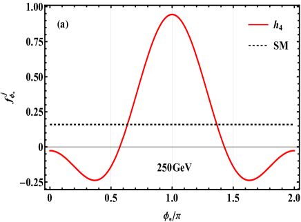
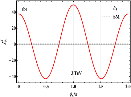
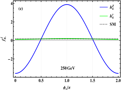
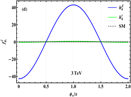
Figure 9: Normalized angular distributions in $\phi_{*}$ for $\hskip 0.85358pte^{+}\hskip 0.85358pte^{-}\!\!\rightarrow\!Z\gamma\hskip 0.85358pt$ with $Z\!\!\rightarrow\!d\hskip 0.85358pt\bar{d}\hskip 0.85358pt$, as generated by $h_{4}$ in our form factor formulation (3.5) in panels $(a)$ and $(b)$, and as generated by $(h_{4}^{Z},\hskip 0.85358pth_{4}^{\gamma})$ in the conventional form factor formulation (3.1) with $h_{5}^{V}\!=0\hskip 0.85358pt$ in panels $(c)$ and $(d)$. The panels $(a)$ and $(c)$ correspond to the $e^{+}e^{-}$ colliders with $\sqrt{s}\!=\!250\,$GeV and the panels $(b)$ and $(d)$ correspond to $\sqrt{s}=3\,$TeV.

Finally, it is instructive to present the $\phi_{*}$ angular distributions for the form factor $h_{4}^{V}$. In the gauge-invariant form factor formulation given in Eq.(3.5), we have imposed the constraints (3.4a)-(3.4b). Hence, the form factor $\hskip 0.85358pth_{5}^{V}\hskip 0.85358pt$ is not independent, and should be replaced by $\hskip 0.85358pth_{5}^{V}\!=-h_{4}^{V}/2\hskip 0.85358pt$, according to Eq.(3.4a). Moreover, Eq.(3.4b) shows that $\hskip 0.85358pth_{4}^{\gamma}\hskip 0.85358pt$ is not independent, so the form factors $(h_{4}^{V},\,h_{5}^{V})$ reduce to a single parameter $\hskip 0.85358pth_{4}\hskip 0.85358pt(\equiv h_{4}^{Z})$ as shown below Eq.(3.4). We can then derive the interference cross section $\sigma_{1}$ contributed by $\hskip 0.85358pth_{4}\hskip 0.85358pt$ and the normalized angular distribution $\hskip 0.85358ptf^{1}_{\phi_{*}}\hskip 0.85358pt$ as follows:

$$\sigma_{1} \,=\,\frac{\leavevmode\nobreak\ e^{2}\!\left(-\mbox{$\frac{\,{1}\,}{2}$}+s_{W}^{2}\right)\!(s\!-\!M_{Z}^{2})\leavevmode\nobreak\ }{8\pi s_{W}c_{W}v^{2}\,s}h_{4}\,,$$ (5.1a)

$$f_{\phi_{*}}^{1} \,=\,\frac{1}{\,2\pi\,}-\frac{\,3\pi(f_{L}^{2}\!-\!f_{R}^{2})(M_{Z}^{2}+5\hskip 0.85358pts)\cos\phi_{*}\,}{256(f_{L}^{2}\!+\!f_{R}^{2})M_{Z}\sqrt{s}}+\frac{\,s\cos 2\phi_{*}\,}{8\pi M_{Z}^{2}}\,.$$ (5.1b)

We see that the interference cross section scales as $\,\sigma_{1}\!\propto\!E^{0}\,$, while the angular distribution $\hskip 0.85358ptf^{1}_{\phi_{*}}\hskip 0.85358pt$ has the leading term $\cos 2\phi_{*}$ enhanced by $E^{2}$ and the subleading term $\cos\phi_{*}$ enhanced by $E^{1}$ for large energy $\sqrt{s\,}\!=\!E\hskip 0.85358pt$. We plot the angular distribution $f_{\phi_{*}}^{1}$ in Fig. 9(a) and 9(b) for the $e^{+}e^{-}$ collider energies $\sqrt{s\,}=250\,$GeV and $3\,$TeV, respectively. In each panel, the $\hskip 0.85358pth_{4}\hskip 0.85358pt$ contribution is depicted by the red solid curve, and the SM contribution is shown as the black dashed curve which is almost flat. We also observe that $\cos\phi_{*}$ and $\cos 2\phi_{*}$ terms in the function $f_{\phi_{*}}^{1}$ in Eq.(5.1b) have opposite signs. They are comparable for lower collision energy $\sqrt{s\,}=250\,$GeV, but $\cos(2\phi_{*})$ becomes dominant for a large collision energy $\sqrt{s\,}=3\,$TeV. We can evaluate the numerical coefficients of $f_{\phi_{*}}^{1}$, as follows:

$$f_{\phi_{*}}^{1} =\,\frac{1}{\,2\pi\,}-0.485\cos\phi_{*}+0.299\cos 2\phi_{*}\hskip 0.85358pt, \text{for}\leavevmode\nobreak\ \sqrt{s\,}=250\hskip 0.85358pt\text{GeV},$$ (5.2a)

$$f_{\phi_{*}}^{1} =\,\frac{1}{\,2\pi\,}-5.67\cos\phi_{*}+43.1\cos 2\phi_{*}\hskip 0.85358pt, \text{for}\leavevmode\nobreak\ \sqrt{s\,}=3\hskip 0.85358pt\text{TeV}.$$ (5.2b)

This explains why panel (a) of Fig. 9 exhibits a significant cancellation between the $\cos\phi_{*}$ and $\cos(2\phi_{*})$ terms, whereas in panel (b) the $\cos(2\phi_{*})$ term dominates and thus the red curve exhibits interesting $\cos(2\phi_{*})$ behavior.

$\sqrt{s\,}$ (TeV)	0.25	0.5	1	3	5
$|h_{4}|$	$3.9\!\times\!10^{-4}$	$3.8\!\times\!10^{-5}$	$4.5\!\times\!10^{-6}$	$1.6\!\times\!10^{-7}$	$3.6\!\times\!10^{-8}$
$|h_{4}^{Z}|$	$8.9\!\times\!10^{-5}$	$4.2\!\times\!10^{-6}$	$2.5\!\times\!10^{-7}$	$3.0\!\times\!10^{-9}$	$3.9\!\times\!10^{-10}$
$|h_{4}^{\gamma}|$	$6.7\!\times\!10^{-4}$	$3.2\!\times\!10^{-5}$	$1.9\!\times\!10^{-6}$	$2.3\!\times\!10^{-8}$	$2.9\!\times\!10^{-9}$

Table 11: Comparisons of the $2\hskip 0.85358pt\sigma$ sensitivities to probing the form factor $\hskip 0.85358pth_{4}\hskip 0.85358pt$ of our SMEFT formulation (3.5) (marked in red color) and the conventional form factors $(h_{4}^{Z},\,h_{4}^{\gamma})$ that take into account only U(1)_em gauge invariance (marked in blue color), as derived by analyzing the reaction $\,e^{+}\hskip 0.85358pte^{-}\!\!\rightarrow\!Z\gamma\!\rightarrow\!q\hskip 0.85358pt\bar{q}\gamma$  at various  $e^{+}e^{-}\!$ colliders with $\mathcal{L}\!=5\,$ab${}^{-1}\!$ and unpolarized $e^{\mp}$ beams. As discussed in the text, the conventional form-factor limits (blue color) are included for illustration only, as they do not respect the full SM gauge symmetry, and hence are invalid.

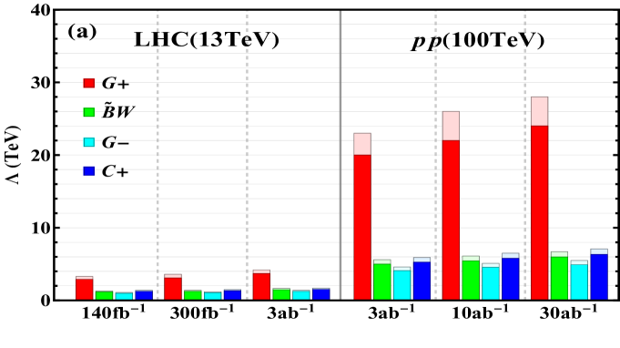
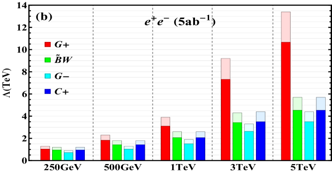
Figure 10: Sensitivity reaches for the new physics scale $\Lambda$ of the nTGC operators at the hadron colliders LHC (13 TeV) and $pp$ (100 TeV) in plot (a) and $e^{+}e^{-}$​ colliders with collision energies $\sqrt{s\,}\!=\!(0.25,\,0.5,\,1,\,3,\,5)$ TeV in plot (b). In each plot, the (${\hskip 1.42262pt}2{\hskip 0.85358pt}\sigma,\,5{\hskip 0.85358pt}\sigma$) sensitivities are shown in (light, heavy) colors, respectively.

For comparison, we consider the conventional form factor formulation (3.1) with $h_{5}^{V}\!=0\hskip 0.85358pt$, where $(h_{4}^{Z},\hskip 0.85358pth_{4}^{\gamma})$ are treated as two independent parameters. In this case we derive the following interference cross sections $(\tilde{\sigma}_{1}^{Z},\hskip 0.85358pt\tilde{\sigma}_{1}^{A})$ contributed by $(h_{4}^{Z},\hskip 0.85358pth_{4}^{\gamma})$ and their normalized angular distributions $\hskip 0.85358pt(\tilde{f}^{1Z}_{\phi_{*}},\hskip 0.85358pt\tilde{f}^{1A}_{\phi_{*}})\hskip 0.85358pt$:

$$(\tilde{\sigma}_{1}^{Z},\,\tilde{\sigma}_{1}^{A}) \,=\,\frac{\leavevmode\nobreak\ e^{4}(s\!-\!M_{Z}^{2})^{2}\leavevmode\nobreak\ }{128\pi M_{Z}^{4}\,s}\left(\!\frac{\,1\!-\!4s_{W}^{2}\,}{s_{W}^{2}c_{W}^{2}}h_{4}^{Z},\leavevmode\nobreak\ \frac{2}{\,s_{W}c_{W}\,}h_{4}^{\gamma}\!\right)\!,$$ (5.3a)

$$\tilde{f}_{\phi_{*}}^{1Z} \,=\,\frac{1}{\,2\pi\,}-\frac{\leavevmode\nobreak\ 3\pi(f_{L}^{2}\!-\!f_{R}^{2})(3s\!+\!M_{Z}^{2})\leavevmode\nobreak\ }{\leavevmode\nobreak\ 128M_{Z}(f_{L}^{2}\!+\!f_{R}^{2})\sqrt{s}\leavevmode\nobreak\ }\frac{\leavevmode\nobreak\ 1\!-\!4s_{W}^{2}\!+\!8s_{W}^{4}\leavevmode\nobreak\ }{1\!-\!4s_{W}^{2}}\cos\phi_{*}\hskip 0.85358pt,$$ (5.3b)

$$\tilde{f}_{\phi_{*}}^{1A} \,=\,\frac{1}{2\pi}-\frac{\leavevmode\nobreak\ 3\pi(f_{L}^{2}\!-\!f_{R}^{2})(3s\!+\!M_{Z}^{2})\leavevmode\nobreak\ }{\leavevmode\nobreak\ 128M_{Z}(f_{L}^{2}+f_{R}^{2})\sqrt{s}\leavevmode\nobreak\ }(1\!-\!4s_{W}^{2})\cos\phi_{*}\hskip 0.85358pt.$$ (5.3c)

We see that the interference cross sections in (5.3) scale as $\,(\tilde{\sigma}_{1}^{Z},\hskip 0.85358pt\tilde{\sigma}_{1}^{A})\!\propto\!E^{2}\,$, while the angular distributions $\hskip 0.85358pt(f^{1Z}_{\phi_{*}},\hskip 0.85358ptf^{1A}_{\phi_{*}})\hskip 0.85358pt$ have leading terms $\propto\cos\phi_{*}$ enhanced by $E^{1}$ for large energy $\sqrt{s\,}\!=\!E^{1}\hskip 0.85358pt$. We also note that the distribution $f^{1A}_{\phi_{*}}$ is much suppressed relative to $f^{1Z}_{\phi_{*}}$ due to the small factor $\,(1-4s_{W}^{2})\!\ll\!1\hskip 0.85358pt$. We plot the angular distributions $\hskip 0.85358pt(f^{1Z}_{\phi_{*}},\hskip 1.42262ptf^{1A}_{\phi_{*}})\hskip 0.85358pt$ of Eq.(5.3c) as the blue solid curves in Fig. 9(c)-(d), while the squared distributions $\hskip 0.85358pt(f^{2Z}_{\phi_{*}},\hskip 0.85358ptf^{2A}_{\phi_{*}})\hskip 0.85358pt$ and the SM distribution $\hskip 0.85358ptf^{0}_{\phi_{*}}\hskip 0.85358pt$ are plotted as the green solid curves and black dashed curves, respectively. As expected, the distributions $\hskip 0.85358pt(f^{2Z}_{\phi_{*}},\hskip 0.85358ptf^{2A}_{\phi_{*}})\hskip 0.85358pt$ and $\hskip 0.85358ptf^{0}_{\phi_{*}}\hskip 0.85358pt$ are dominated by the constant term and thus nearly flat.

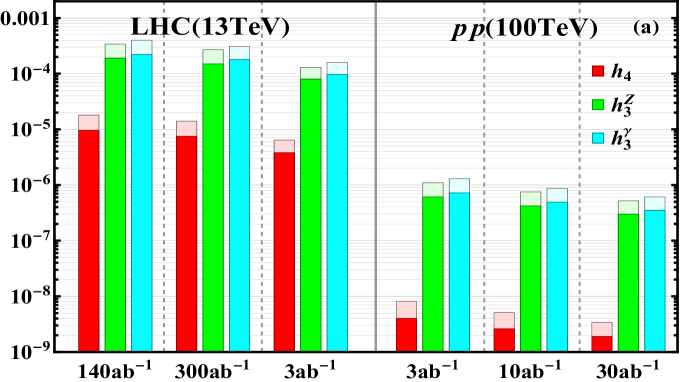
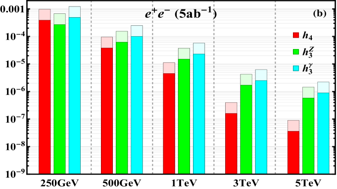
Figure 11: Sensitivity reaches for the nTGC form factors $(h_{4},\,h_{3}^{Z},\,h_{3}^{\gamma})$ at the hadron colliders LHC (13 TeV) and $pp$ (100 TeV) in plot (a) and at $e^{+}e^{-}$​ colliders with collision energies $\sqrt{s\,}\!=\!(0.25,\,0.5,$ $\,1,\,3,\,5)$ TeV in plot (b). In each plot, the ($\,2{\hskip 0.85358pt}\sigma,\,5{\hskip 0.85358pt}\sigma$) sensitivities are shown in (heavy, light) colors, respectively.

We stress that Eq.(5.3) and the corresponding Figs. 9(c)-(d) are incorrect because the conventional form factor formulation (3.1) with $\,h_{5}^{V}\!=0\,$ does not obey the consistency conditions (3.4) imposed by the spontaneous breaking of the electroweak gauge symmetry SU(2)${}_{L}\otimes$U(1)_Y of the SMEFT. In the following we further show that the conventional form factor formulation also leads to erroneously strong sensitivity limits on the form factors $(h_{4}^{Z},\,h_{4}^{\gamma})$.

Following the steps leading to Eq.(4.11), we construct the following observables $(\mathbb{O}_{1},\,\mathbb{\widetilde{O}}_{1})$ for probing the form factors:

$$\mathbb{O}_{1} \,=\,\left|\hskip 0.85358pt\sigma_{1}\!\int\!\!\mathrm{d}\phi_{*}\,f_{\phi_{*}}^{1}\!\times\text{sign}(\cos 2\phi_{*})\right|,$$ (5.4a)

$$\mathbb{\widetilde{O}}_{1} \,=\,\left|\hskip 0.85358pt\tilde{\sigma}_{1}\!\int\!\!\mathrm{d}\phi_{*}\,\tilde{f}_{\phi_{*}}^{1}\!\times\text{sign}(\cos\phi_{*})\right|.$$ (5.4b)

From the above formulae (5.1a) and (5.3), we deduce that energy-dependences of the observables are $\hskip 0.85358pt\mathbb{O}_{1}(h_{4})\!\propto\!E^{2}\hskip 0.85358pt$ and $\hskip 0.85358pt\mathbb{\widetilde{O}}_{1}(h_{4}^{V})\!\propto\!E^{3}\hskip 0.85358pt$. This shows that in the conventional form factor formulation $\mathbb{\widetilde{O}}_{1}^{c}$ has an erroneously large energy-dependence ($E^{3}$ instead of $E^{2}$), leading to incorrectly strong sensitivities to the form factors $(h_{4}^{Z},\,h_{4}^{\gamma})$. We present these incorrect sensitivities in blue color in Table 11. For comparison, we also show in this Table the correct sensitivities (red color) to the form factors $h_{4}$, as derived within our consistent form factor formulation (3.5) with the constraints (3.4a) and (3.4b). From this comparison, we see that for the form factor $\hskip 0.85358pth_{4}^{Z}\hskip 0.85358pt$ the conventional sensitivities (blue color) are erroneously stronger than our new sensitivities (red color) by a factor of $5$ for the collider energy $\sqrt{s\,}=250$ GeV, by a factor of $\,{O}(10-20)$ for the collider energies $\sqrt{s\,}=(0.5-1)$ TeV, and by a factor of ${O}(10^{2})$ for the collider energies $\sqrt{s\,}=(3-5)$ TeV.

Finally, for an intuitive comparison and overview, we summarize in Fig. 10 the sensitivity reaches for the new physics scales of the dimension-8 nTGC operators at the hadron colliders [panel (a)] and the $e^{+}e^{-}$ colliders [panel (b)] from Tables 4-5 and Table 9. We present these limits at both the $(2{\hskip 0.85358pt}\sigma,\hskip 0.85358pt5{\hskip 0.85358pt}\sigma)$ levels, which are indicated by the (light, heavy) colors respectively. In Fig. 10(b) we only plot the sensitivity reaches for $e^{-}e^{+}$ collisions with unpolarized electron/positron beams. We note that according to Table 9, adding the $e^{-}/e^{+}$ beam polarizations can increase the sensitivity reaches on the new physics scale by about $20\%$ for $\mathcal{O}_{G+}$ and $\mathcal{O}_{C+}$, and by about $5\%$ for $\mathcal{O}_{\widetilde{B}W}$. Also, we summarize in Fig. 11 the sensitivity reaches for probing the nTGC form factors $(h_{4},\hskip 0.85358pth_{3}^{Z},\hskip 0.85358pth_{3}^{\gamma})$ at the hadron colliders [panel (a)] and the $e^{+}e^{-}$ colliders [panel (b)] from Table 7 and Table 10, where the $(2{\hskip 0.85358pt}\sigma,\hskip 0.85358pt5{\hskip 0.85358pt}\sigma)$ limits are marked by the (light, heavy) colors, respectively. In Fig. 10(b) we present only the sensitivity reaches for $e^{-}e^{+}$ collisions with unpolarized electron/positron beams. We note that according to Table 10, adding the $e^{-}/e^{+}$ beam polarizations can increase the sensitivity reaches for the nTGC form factors by about $100\%$ for $h_{4}$, by about $20\%$ for $h_{3}^{Z}$, and by about $160\%$ for $h_{3}^{\gamma}$.

The reason that the effects of beam polarization for probing the nTGC form factors in $e^{-}e^{+}$ collisions appear much stronger than those for probing the new physics cutoff scales of the dimension-8 nTGC operators can be understood as follows. We note that the relation between the polarized and unpolarized cross sections of the SM backgrounds is given by [5]:

$$\sigma_{0}(P_{L}^{e},P_{R}^{\bar{e}}) \!\!=\!\! 4\frac{\,P_{L}^{e}P_{R}^{\bar{e}}c_{L}^{2}\!+\!(1\!-\!P_{L}^{e})(1\!-\!P_{R}^{\bar{e}})c_{R}^{2}\,}{c_{L}^{2}\!+c_{R}^{2}}\,\sigma_{0}(0.5,0.5)\,,$$ (5.5)

where $P_{L}^{e}$ $(P_{R}^{\bar{e}})$ denotes the fraction of left-handed (right-handed) electrons (positrons) in the $e^{-}$ ($e^{+}$) beam and $\hskip 0.85358ptP_{L}+\!P_{R}=\!1\hskip 0.85358pt$ holds for both $e^{-}$ and $e^{+}$ beams.

According to Ref. [5], we construct the following three kinds of $\mathbb{O}_{1}$ observables and extract the different signal terms of $O(\Lambda^{-4})$ in the differential cross section:

$$\mathbb{O}_{A} \!\!=\!\! \int\!\!\mathrm{d}\theta\mathrm{d}\theta_{*}\mathrm{d}\phi_{*}\,\frac{d^{3}\sigma_{1}}{\mathrm{d}\theta\mathrm{d}\theta_{*}\mathrm{d}\phi_{*}}\text{sign}(\cos\!\phi_{*})\,,$$ (5.6a)

$$\mathbb{O}_{B} \!\!=\!\! \int\!\!\mathrm{d}\theta\mathrm{d}\theta_{*}\mathrm{d}\phi_{*}\,\frac{d^{3}\sigma_{1}}{\mathrm{d}\theta\mathrm{d}\theta_{*}\mathrm{d}\phi_{*}}\text{sign}(\cos\!\phi_{*})\text{sign}(\cos\!\theta)\text{sign}(\cos\!\theta_{*})\,,$$ (5.6b)

$$\mathbb{O}_{C} \!\!=\!\! \int\!\!\mathrm{d}\theta\mathrm{d}\theta_{*}\mathrm{d}\phi_{*}\,\frac{d^{3}\sigma_{1}}{\mathrm{d}\theta\mathrm{d}\theta_{*}\mathrm{d}\phi_{*}}\text{sign}(\cos\!2\phi_{*})\,.$$ (5.6c)

For these observables, we can deduce the following:

$$\mathbb{O}_{A}(G+) \!\!=\!\! \mathbb{A}\times\mbox{$\frac{\,{1}\,}{2}$}c_{L}P_{L}^{e}P_{R}^{\bar{e}}(5s\!+\!M_{Z}^{2})\Lambda^{-4}_{G+}\,,$$ (5.7a)

$$\mathbb{O}_{A}(j) \!\!=\!\! \mathbb{A}\times 3\!\left[c_{L}x_{L}P_{L}^{e}P_{R}^{\bar{e}}\!+\!c_{R}x_{R}(1\!-\!P_{L}^{e})(1\!-\!P_{R}^{\bar{e}})\right]\!(s\!+\!M_{Z}^{2})\Lambda^{-4}_{j}\,,$$ (5.7b)

$$\mathbb{O}_{B}(G+) \!\!=\!\! \mathbb{B}\times\mbox{$\frac{\,{1}\,}{2}$}c_{L}P_{L}^{e}P_{R}^{\bar{e}}(5s\!+\!M_{Z}^{2})\Lambda^{-4}_{G+}\,,$$ (5.7c)

$$\mathbb{O}_{B}(j) \!\!=\!\! \mathbb{B}\times 3\!\left[c_{L}x_{L}P_{L}^{e}P_{R}^{\bar{e}}\!-\!c_{R}x_{R}(1\!-\!P_{L}^{e})(1\!-\!P_{R}^{\bar{e}})\right]\!(s\!+\!M_{Z}^{2})\Lambda^{-4}_{j}\,,$$ (5.7d)

$$\mathbb{O}_{C}(G+) \!\!=\!\! \mathbb{C}\times\mbox{$\frac{\,{1}\,}{2}$}c_{L}P_{L}^{e}P_{R}^{\bar{e}}\,s\,\Lambda^{-4}_{G+}\,,$$ (5.7e)

$$\mathbb{O}_{C}(j) \!\!=\!\! \mathbb{C}\times\!\left[c_{L}x_{L}P_{L}^{e}P_{R}^{\bar{e}}\!-\!c_{R}x_{R}(1\!-\!P_{L}^{e})(1\!-\!P_{R}^{\bar{e}})\right]\!M_{Z}^{2}\Lambda^{-4}_{j}\,,$$ (5.7f)

where the index $j$ denotes the operators $(\mathcal{O}_{G-},\hskip 0.85358pt\mathcal{O}_{\widetilde{B}W},\hskip 0.85358pt\mathcal{O}_{C+})$, respectively. The values of the coefficients $(\mathbb{A},\hskip 0.85358pt\mathbb{B},\hskip 0.85358pt\mathbb{C})$ in these formulae are given by the numerical results for the observables in Eq.(5.6). The dependence of each sensitivity limit on the polarization choice is determined by the relation between the left- and right-handed couplings. The most sensitive observable for probing $\mathcal{O}_{G+}\,(h_{4})$ is $\mathbb{O}_{C}$, while the most sensitive observable for probing $\mathcal{O}_{\widetilde{B}W}\,(h_{3}^{Z})$ and $\mathcal{O}_{C+}$ is $\mathbb{O}_{A}$. For probing $\mathcal{O}_{G-}\,(h_{3}^{\gamma})$, the most sensitive observable is $\mathbb{O}_{B}$ in the case of unpolarized beams, and is $\mathbb{O}_{A}$ in the case of polarized beams [for the choice $(P_{L}^{e},\hskip 0.85358ptP_{R}^{\bar{e}})\!=\!(0.9,\hskip 0.85358pt0.65)$]. We note that the sensitivity limits for the nTGC form factors scale as $\,(h_{3}^{V},\hskip 0.85358pth_{4}^{V})\!\propto\!\mathbb{O}_{X}$ (where $X\!=\!A,B,C$), and that the new physics cutoff reaches of the dimension-8 nTGC operators behave like $\Lambda\!\propto\!\mathbb{O}_{X}^{1/4}$. Hence, the improvements from the beam polarizations can be significant for the form factors, but become rather mild for the cutoff scales of the dimension-8 operators.

For convenience, we express a given observable $\,\mathbb{O}_{X}\!\equiv\overline{\mathbb{O}}_{X}/\Lambda_{j}^{4}\,$ for the dimension-8 operator formulation and $\,\mathbb{O}_{X}\!\equiv\overline{\mathbb{O}}_{X}h_{i}^{V}\,$ for the form factor formulation. We may estimate the significance by $\,\mathcal{Z}\!\simeq\!S/\!\sqrt{B\,}$.  If we require the significances of the polarized and unpolarized cases to be equal, $\mathcal{Z}_{\mathrm{pol}}\!=\!\mathcal{Z}_{\mathrm{unpol}}\hskip 0.85358pt$, we can derive the following ratio of the polarized/unpolarized limits on the dimension-8 cutoff scales and on the form factors, respectively:

$$\mathcal{R}_{\Lambda_{j}}=\frac{\Lambda_{j}(\mathrm{pol})}{\,\Lambda_{j}(\mathrm{unpol})\,}=\big{[}\overline{\mathcal{R}}_{X}(P_{L}^{e},P_{R}^{\bar{e}})\big{]}^{\!1/4},\leavevmode\nobreak\ \leavevmode\nobreak\ \leavevmode\nobreak\ \leavevmode\nobreak\ \mathcal{R}_{h_{i}^{V}}=\frac{\,h_{i}^{V}\!(\mathrm{unpol})\,}{h_{i}^{V}\!(\mathrm{pol})}=\overline{\mathcal{R}}_{X}(P_{L}^{e},P_{R}^{\bar{e}})\hskip 0.85358pt,$$ (5.8)

where the ratio $\overline{\mathcal{R}}_{X}(P_{L}^{e},P_{R}^{\bar{e}})$ is defined as

$$\overline{\mathcal{R}}_{X}(P_{L}^{e},P_{R}^{\bar{e}})\hskip 0.85358pt\equiv\hskip 0.85358pt\frac{\,\overline{\mathbb{O}}_{X}(P_{L}^{e},P_{R}^{\bar{e}})\,}{\leavevmode\nobreak\ \overline{\mathbb{O}}_{X}(0.5,0.5)\,}\sqrt{\frac{\,\sigma_{0}(0.5,0.5)\,}{\sigma_{0}(P_{L}^{e},P_{R}^{\bar{e}})}\,}\hskip 0.85358pt.$$ (5.9)

From the above, we derive the following estimate of the ratio $\overline{\mathcal{R}}_{X}$ for each observable $\mathbb{O}_{X}$:

$$\overline{\mathcal{R}}_{A}\! \!\!=\!\! \frac{\,2\hskip 0.85358pt\big{|}c_{L}x_{L}P_{L}^{e}P_{R}^{\bar{e}}+c_{R}x_{R}(1\!-\!P_{L}^{e})(1\!-\!P_{R}^{\bar{e}})\big{|}\,}{|c_{L}x_{L}+c_{R}x_{R}|}\sqrt{\frac{c_{L}^{2}\!+c_{R}^{2}}{\,P_{L}^{e}P_{R}^{\bar{e}}c_{L}^{2}\!+\!(1\!-\!P_{L}^{e})(1\!-\!P_{R}^{\bar{e}})c_{R}^{2}\,}}\hskip 0.85358pt,\hskip 34.1433pt$$ (5.10a)

$$\overline{\mathcal{R}}_{B,C}\! \!\!=\!\! \frac{\,2\hskip 0.85358pt\big{|}c_{L}x_{L}P_{L}^{e}P_{R}^{\bar{e}}-c_{R}x_{R}(1\!-\!P_{L}^{e})(1\!-\!P_{R}^{\bar{e}})\big{|}\,}{|c_{L}x_{L}-c_{R}x_{R}|}\sqrt{\frac{c_{L}^{2}\!+c_{R}^{2}}{\,P_{L}^{e}P_{R}^{\bar{e}}c_{L}^{2}+(1\!-\!P_{L}^{e})(1\!-\!P_{R}^{\bar{e}})c_{R}^{2}\,}},$$ (5.10b)

where $(c_{L},\hskip 0.85358ptc_{R})\!=\!(T_{3}-Qs_{W}^{2},-Qs_{W}^{2})$ denote the $Z$ coupling factors with the (left, right)-handed electrons, and the coupling coefficients $(x_{L},\hskip 0.85358ptx_{R})$ are given by

$$(x_{L},\,x_{R}) \,=\,-Qs_{W}^{2}(1,\,1)\hskip 0.85358pt, (\hskip 0.85358pt\text{for}\leavevmode\nobreak\ \mathcal{O}_{G-}\hskip 0.85358pt)\hskip 0.85358pt,$$ (5.11a)

$$(x_{L},\,x_{R}) \,=\,(T_{3}\!-\!Qs_{W}^{2},\,-Qs_{W}^{2})\hskip 0.85358pt, (\hskip 0.85358pt\text{for}\leavevmode\nobreak\ \mathcal{O}_{\!\widetilde{B}W}\hskip 0.85358pt)\hskip 0.85358pt,$$ (5.11b)

$$(x_{L},\,x_{R}) \,=\,-T_{3}(1,0), (\hskip 0.85358pt\text{for}\leavevmode\nobreak\ \mathcal{O}_{G+},\mathcal{O}_{C+}\hskip 0.85358pt)\hskip 0.85358pt.$$ (5.11c)

Because the coupling coefficient $x_{R}\!=0\hskip 0.85358pt$ for $\mathcal{O}_{G+}(h_{4})$ and $\mathcal{O}_{C+}$, we can reduce the significance ratio (5.10) to the following form and compute its value for $(P_{L}^{e},P_{R}^{\bar{e}})\!=\!(0.9,0.65)$:

$$\overline{\mathcal{R}}_{X}(P_{L}^{e},P_{R}^{\bar{e}})\!\! = \!\!2P_{L}^{e}P_{R}^{\bar{e}}\sqrt{\frac{c_{L}^{2}\!+c_{R}^{2}}{\,P_{L}^{e}P_{R}^{\bar{e}}c_{L}^{2}\!+\!(1\!-\!P_{L}^{e})(1\!-\!P_{R}^{\bar{e}})c_{R}^{2}\,}},$$ (5.12a)

$$\overline{\mathcal{R}}_{X}(0.9,0.65)\!\!\! \simeq \!\!2.0\hskip 0.85358pt,$$ (5.12b)

where $X\!=\!A,B,C$. Thus, we deduce the following ratios for the operators $(\mathcal{O}_{G+},\mathcal{O}_{C+})$ and the form factor $h_{4}$:

$$\overline{\mathcal{R}}_{\Lambda_{G+}}\!\!\!\! = \!\!\overline{\mathcal{R}}_{\Lambda_{C+}}\!=\,\big{[}\overline{\mathcal{R}}_{X}(0.9,0.65)\big{]}^{1/4}\simeq 1.2\hskip 0.85358pt,$$ (5.13a)

$$\overline{\mathcal{R}}_{h_{4}}\!\!\!\! = \!\!\!\overline{\mathcal{R}}_{X}(0.9,0.65)\simeq 2.0\hskip 0.85358pt.$$ (5.13b)

This means that the $e^{-}/e^{+}$ beam polarizations can enhance the sensitivity reach for the cutoff scale $\Lambda_{G+}$ by about 20%, and enhance the sensitivity reach for the form factor $h_{4}$ much more significantly, namely by about 100%, which explains the features shown in Tables 9-10 and Figs. 10-11.

We further note that the coupling coefficients $x_{L,R}\!=\!c_{L,R}$ for the nTGC operator $\mathcal{O}_{\widetilde{B}W}$ and form factor $h_{3}^{Z}$. We find that to enhance the polarization effects for probing $\mathcal{O}_{\widetilde{B}W}$ and $h_{3}^{Z}$, the most sensitive observable is $\mathbb{O}_{A}$.  Thus, we simplify the significance ratio (5.10) to the following form and compute its value for $(P_{L}^{e},P_{R}^{\bar{e}})\!=\!(0.9,0.65)$:

$$\overline{\mathcal{R}}_{A}(P_{L}^{e},P_{R}^{\bar{e}}) =\,2\hskip 0.85358pt\sqrt{\frac{\,P_{L}^{e}P_{R}^{\bar{e}}c_{L}^{2}\!+\!(1\!-\!P_{L}^{e})(1\!-\!P_{R}^{\bar{e}})c_{R}^{2}\leavevmode\nobreak\ }{c_{L}^{2}\!+c_{R}^{2}}},$$ (5.14)

$$\overline{\mathcal{R}}_{A}(0.9,0.65) \simeq 1.2\,.$$ (5.15)

With these, we deduce the following ratios for the operator $\mathcal{O}_{\widetilde{B}W}$ and the form factor $h_{3}^{Z}$:

$$\overline{\mathcal{R}}_{\Lambda_{\widetilde{B}W}}\!\!\!\! = \!\!\big{[}\overline{\mathcal{R}}_{A}(0.9,0.65)\big{]}^{1/4}\simeq 1.05\hskip 0.85358pt,$$ (5.16a)

$$\overline{\mathcal{R}}_{h_{3}^{Z}}\!\!\!\! = \!\!\!\overline{\mathcal{R}}_{X}(0.9,0.65)\simeq 1.2\,.$$ (5.16b)

This shows that the beam polarizations can increase mildly the sensitivity reach for the cutoff scale $\Lambda_{\widetilde{B}W}$ by about 5%, and increase the sensitivity reach for the form factor $h_{3}^{Z}$ by a larger amount of 20%, which agree with the features shown in Tables 9-10 and Figs. 10-11. Finally, we note that the enhancement ratio (5.9) does not apply to the cases of $\mathcal{O}_{G-}$ and $h_{3}^{\gamma}$ because there $\mathbb{O}_{B}$ is the most sensitive observable for the unpolarized case and $\mathbb{O}_{A}$ is the most sensitive observable for the polarized case. Thus, we define the corresponding ratio $\mathcal{R}_{AB}(P_{L}^{e},P_{R}^{\bar{e}})$ of significances between the polarized and unpolarized cases and compute its value $\mathcal{R}_{AB}(0.9,0.65)$:

$$\overline{\mathcal{R}}_{AB}(P_{L}^{e},P_{R}^{\bar{e}}) \simeq\frac{\,\overline{\mathbb{O}}_{A}(P_{L}^{e},P_{R}^{\bar{e}})\,}{\leavevmode\nobreak\ \overline{\mathbb{O}}_{B}(0.5,0.5)\,}\sqrt{\frac{\,\sigma_{0}(0.5,0.5)\,}{\sigma_{0}(P_{L}^{e},P_{R}^{\bar{e}})}\,}\hskip 0.85358pt,$$ (5.17a)

$$\overline{\mathcal{R}}_{AB}(0.9,0.65) \simeq 2.6\,.$$ (5.17b)

From these we derive the significance ratios for the operator $\mathcal{O}_{G-}$ and the form factor $h_{3}^{\gamma}$:

$$\mathcal{R}_{\Lambda_{G-}}\!\!\!\! = \!\!\big{[}\overline{\mathcal{R}}_{AB}(0.9,0.65)\big{]}^{1/4}\simeq 1.27\hskip 0.85358pt,$$ (5.18a)

$$R_{h_{3}^{\gamma}}\!\!\!\! = \!\!\!\overline{\mathcal{R}}_{X}(0.9,0.65)\simeq 2.6\,.$$ (5.18b)

We see that the beam polarization effects can raise the sensitivity reach for the cutoff scale $\Lambda_{G-}$ by about 27%, and raise the sensitivity reach for the form factor $h_{3}^{\gamma}$ by about 160%, which agree with the results presented in Tables 9-10 and Figs. 10-11.

6 Conclusions

Neutral triple-gauge couplings (nTGCs) provide an important window for probing new physics beyond the SM. In this work, we have studied systematically the prospective experimental sensitivities to nTGCs at the 13 TeV LHC and a future 100 TeV $pp$ collider, using the SMEFT approach to classify and characterize the nTGCs that can arise from gauge-invariant dimension-8 operators.

In Section 2.1 we first considered a set of CP-conserving dimension-8 nTGC operators and the related contact operators in Eq.(2.2). Then, in Section 2.2 we derived their contributions to the scattering amplitudes of the partonic process $\bar{q}{\hskip 0.85358pt}q\!\rightarrow\!Z\gamma\hskip 0.85358pt$ in Eqs.(2.7) and (2.8). With these, we computed the corresponding total cross sections including the SM contribution, the interference term of $O(1/\Lambda^{4})$, and the squared term of $O(1/\Lambda^{8})$, as in Eqs.(2.2) and (2.2), where $\Lambda$ is the new physics cutoff scale defined in Eq.(2.1). We further presented in Eq.(2.14), Eq.(2.17), and Fig. 3 their contributions to the differential angular distributions, in comparison with that of the SM. In Section 2.3 we analyzed the perturbative unitarity bounds on the nTGCs, as shown in Table 1 and Fig. 1, which are much weaker than the collider limits presented in Sections 4-5. Hence, the perturbation expanison is well justified for the current collider analyses.

In Section 3 we presented a new form factor formulation of the neutral triple gauge vertices (nTGVs) $Z\gamma V^{*}$ (with $V\!=\!Z,\gamma$), by mapping them to the dimension-8 nTGC operators of the SMEFT that incorporate the spontaneously-broken electroweak gauge symmetry SU(2)${}_{\mathrm{L}}\otimes$U(1)_Y of the SM. This differs from the conventional form factor parametrization of nTGCs that takes into account only the unbroken U(1)_em gauge symmetry [3][4]. Using the SMEFT approach, we have found that a new momentum-dependent nTGC term with form factor $h_{5}^{V}$ has to be added and the mapping with the dimension-8 SMEFT interactions enforces new nontrivial relations (3.4a)-(3.4b) between the form factors $(h_{4}^{V},\hskip 0.85358pth_{5}^{V})$ and between the form factors $(h_{4}^{Z},\,h_{4}^{\gamma})$. The new form factor $h_{5}^{V}$ was not included in all the previous form factor analyses of nTGVs. We have demonstrated that including the new form factor $h_{5}^{V}$ is crucial for a fully consistent form factor formulation of nTGVs and ensures the exact cancellation of the spuriously large unphysical terms of $O(E^{5})$ in the scattering amplitudes of $\hskip 0.85358ptq{\hskip 0.85358pt}\bar{q}\!\rightarrow\!Z\gamma\hskip 0.85358pt$, as shown in Eqs.(3.8b) and (3.10). In consequence, among the six general nTGC form factors $(h_{3}^{V},\,h_{4}^{V},\,h_{5}^{V})$ in Eq.(3.2), we have proven that only three of them, $(h_{3}^{Z},\,h_{3}^{\gamma},\,h_{4})$ with $\hskip 0.85358pth_{4}\!\equiv\!h_{4}^{Z}\hskip 0.85358pt$, are independent, and the correct nTGC form factor formula is given by Eq.(3.5). We have further presented the explicit correspondence between the nTGC form factors and the cutoff scales of the dimension-8 nTGC operators in Eqs.(3.6)-(3.7).

In Section 4, we have systematically studied the sensitivity reaches for probing the new physics scales of the nTGC operators and for probing the nTGC form factors in the reactions $\,pp\hskip 0.85358pt(q{\hskip 0.85358pt}\bar{q})\!\rightarrow\!Z\gamma\!\rightarrow\!\ell\bar{\ell}\gamma,\hskip 0.85358pt\nu\bar{\nu}\gamma$  at the LHC and the future $pp$ (100 TeV) collider. We have presented analyses of sensitivity reaches using the interference contributions of $O(\Lambda^{-4})$ in Section 4.2 and including the squared contributions up to $O(\Lambda^{-8})$ in Section 4.3. We have evaluated the prospective $2{\hskip 0.85358pt}\sigma$ and $5{\hskip 0.85358pt}\sigma$ sensitivities of the LHC and the future 100 TeV $pp$ collider to the different nTGCs, and have combined the sensitivity reaches of the leptonic decay channel $Z\!\rightarrow\!\ell^{+}\ell^{-}$ (Secs. 4.2-4.3) and the invisible decay channel $Z\!\rightarrow\!\nu{\hskip 0.85358pt}\bar{\nu}\hskip 0.85358pt$ (Sec. 4.4). We have presented our findings in Tables 2 to 4 for the dimension-8 operator $\hskip 0.85358pt\mathcal{O}_{G+}$ and the equivalent operator $\hskip 0.85358pt\mathcal{O}_{C-}$, and in Table 5 for the other dimension-8 operators $(\mathcal{O}_{\widetilde{B}W},\,\mathcal{O}_{G-},\,\mathcal{O}_{C+})$. These sensitivity reaches are further summarized in our Fig. 10(a). From Table 4, we see that the $2{\hskip 0.85358pt}\sigma$ ($5{\hskip 0.85358pt}\sigma$) sensitivity to the scale of the operator $\mathcal{O}_{G+}$ could reach 4.4 TeV (3.9 TeV) at the 13 TeV LHC with 3 ab^-1 integrated luminosity, and reach 30 TeV (26 TeV) at the 100 TeV $pp$ collider with 30 ab^-1, whereas the estimated sensitivity reaches on the scales of the dimension-8 operators $(\mathcal{O}_{\widetilde{B}W},\,\mathcal{O}_{G-},\,\mathcal{O}_{C+})$ shown in Table 5 are somewhat smaller. Then, in Section 4.5 we have presented the LHC sensitivity reaches on the three independent form factors $(h_{4},\,h_{3}^{Z},\,h_{3}^{\gamma})\hskip 0.85358pt$ in Table 7, with a summary of these sensitivities given in Fig. 11(a). We see that the sensitivities for probing the form factor $h_{4}$ are generally higher than those of the other two form factors $(h_{3}^{Z},\,h_{3}^{\gamma})$ by about a factor of $5\!\times\!10^{-2}$ at the LHC and by about a factor of $10^{-2}$ at the 100 TeV $pp$ collider. We emphasise that if the dimension-8 SMEFT relations between the different form factors are not taken into account, one would find unrealistically strong sensitivities due to the uncancelled large unphysical energy-dependent terms associated with the form factor $h_{4}\hskip 0.85358pt$, as seen by comparing Eq.(4.20) with Eq.(4.17). Then, we explicitly demonstrated in Table 8 that the sensitivities to $h_{4}^{Z}$ and $h_{4}^{\gamma}$ in the conventional form factor approach (marked in blue color) are (erroneously) higher than the correct sensitivities (marked in red color and extracted from Table 7) by about a factor of $5\!\times\!10^{-2}$ at the LHC and by about a factor of $10^{-2}$ at the $pp$ (100 TeV) collider. Hence, it is important to use the consistent form factor approach for the nTGC analysis as we advocated in Section 3. After these comparisons, in Section 4.6 we analyzed the 2-parameter correlations for both the nTGC form factors and for the nTGC dimension-8 operators. We presented in Fig.5 the correlations of each pair of the form factors $(h_{4},\hskip 0.85358pth_{3}^{V})$ and $(h_{3}^{Z},\hskip 0.85358pth_{3}^{\gamma})$ at hadron colliders, where the $(h_{4},\hskip 0.85358pth_{3}^{V})$ contours in the plots (a) and (b) have rather weak correlations due to the extra energy-suppression factor of Eq.(4.33), and the plots (c) and (d) demonstrate large correlations between the form factors $(h_{3}^{Z},\hskip 0.85358pth_{3}^{\gamma})$. Then, we presented the correlations of each pair of the nTGC operators $(\mathcal{O}_{G+},\,\mathcal{O}_{\widetilde{B}W})$ and $(\mathcal{O}_{G+},\,\mathcal{O}_{G-})$ in Figs. 6(a)-(b) which are suppressed by large energy factor $\hskip 0.85358pt1/\!\sqrt{\bar{s}\,}\,$ as shown in Eq.(4.37). The correlations of each pair of the nTGC operators $(\mathcal{O}_{\widetilde{B}W},\,\mathcal{O}_{G-})$, $(\mathcal{O}_{C+},\,\mathcal{O}_{\widetilde{B}W})$, and $(\mathcal{O}_{C+},\,\mathcal{O}_{G-})$ are presented in Figs. 7(a) to (d). These correlations are not suppressed by any energy factor and are thus significant at both the LHC and the 100 TeV $pp$ collider. We demonstrated in Figs. 7(c)-(d) that the correlations of the operators $(\mathcal{O}_{C+},\,\mathcal{O}_{\widetilde{B}W})$ and $(\mathcal{O}_{C+},\,\mathcal{O}_{G-})$ are particularly strong. Finally, in Section 4.7 we have made direct comparison with the published LHC measurements on nTGCs in the reaction $\hskip 0.85358ptp{\hskip 0.85358pt}p{\hskip 0.85358pt}(q{\hskip 0.85358pt}\bar{q})\!\rightarrow\!Z\gamma\hskip 0.85358pt$ (with $Z\!\!\rightarrow\!\nu{\hskip 0.85358pt}\bar{\nu}{\hskip 0.85358pt})$ by the CMS [18] and ATLAS [19] collaborations. Using the same kinematic cuts and integrated luminosity together with an estimated detection efficiency as in the ATLAS analysis [19], we have applied the conventional form factor formula (3.1) to reproduce the nTGC bounds in Eq.(4.52) and the strong correlations of $(h_{3}^{V},\hskip 0.85358pth_{4}^{V})$ in Figs. 8(c)-(d), which agree well with the ATLAS results [19]. However, the $(h_{3}^{V},\hskip 0.85358pth_{4}^{V})$ contours of Figs. 8(c)-(d) differ substantially from those contours of Figs. 8(a)-(b), which exhibit rather weak correlations as predicted using our new SMEFT form factor formula (3.5). Hence, it is important to use the SMEFT form factor formulation described in Section 3 to analyze the LHC bounds on nTGCs.

We presented in Section 5 systematic comparisons of the sensitivity reaches for the nTGCs between the hadron colliders (the LHC and the 100 TeV $\!pp$ collider) and $e^{+}e^{-}$ colliders with different energies. Table 9 summarizes the comparisons for probing the nTGCs of dimension-8 operators $(\mathcal{O}_{G+},\,\mathcal{O}_{\widetilde{B}W},\,\mathcal{O}_{G-},\,\mathcal{O}_{C+})$, whereas Table 10 summarizes the comparisons for probing the nTGC form factors $(h_{4},\,h_{3}^{Z},\,h_{3}^{\gamma})$. We have summarized the above comparisons of sensitivity reaches between the hadron colliders and lepton colliders in Figs. 6 and 10. Then, in Table 11, we have further demonstrated that using naively the conventional form factor formula without including the nontrivial constraints of the dimension-8 SMEFT approach would cause erroneous sensitivities to $(h_{4}^{Z},\,h_{4}^{\gamma})$ (marked in blue color) that are stronger than the correct sensitivities (marked in red color and extracted from Table 10) at the $e^{+}e^{-}$ colliders by a factor of $\hskip 0.85358ptO(10)\hskip 0.85358pt$ for the collision energy $\sqrt{s\,}\!\leqslant\!1$ TeV and by a factor of $\hskip 0.85358ptO(10^{2})\hskip 0.85358pt$ for $\sqrt{s\,}=(3-5)\hskip 0.85358pt$TeV. Hence, it is important to use the consistent form factor approach of Section 3 for nTGC analyses at $e^{+}e^{-}$ colliders. In general, from the comparisons of Tables 9-10 and Figs. 10-11, we find that the LHC sensitivity reaches on the nTGCs are similar to those at the $e^{+}e^{-}$ colliders with collision energy $\sqrt{s\,}\!\leqslant\!1$ TeV [5]. On the other hand, a higher-energy $e^{+}e^{-}$ collider with $\sqrt{s\,}=\!(3\!-\!5)\hskip 0.85358pt$TeV would have greater sensitivities than the LHC to probing the new physics scales of the nTGC operators and the corresponding nTGC form factors. However, we have shown that the sensitivity reaches of the 100 TeV $pp\hskip 0.85358pt$ collider would be even higher.

Overall, we have found that nTGCs provide a powerful means for probing any possible new physics beyond the SM that could generate the dimension-8 nTGC operators in the SMEFT. We have found that both $\hskip 0.85358ptpp\hskip 0.85358pt$ and $e^{+}e^{-}$ colliders have significant roles to play. We advocate as a first step that the ATLAS and CMS experiments at the LHC apply the dimension-8 SMEFT approach proposed here to analyze the nTGCs, in preference to the conventional form factor approach that does not take into account the full electroweak gauge symmetry SU(2)${}_{\mathrm{L}}\otimes\hskip 0.85358pt$U(1)_Y of the SM.

Acknowledgements
The work of JE was supported in part by United Kingdom STFC Grants ST/P000258/1 and ST/T000759/1, in part by the Estonian Research Council via a Mobilitas Pluss grant, and in part by the TDLI distinguished visiting fellow programme. The work of HJH and RQX was supported in part by the National NSF of China (under grants Nos. 11835005 and 12175136) and by the National Key R & D Program of China (No. 2017YFA0402204). RQX has been supported by an International Postdoctoral Exchange Fellowship.

References

- [1] For recent reviews, John Ellis, arXiv:2105.14942 [hep-ph], in the conference proceedings of “Beyond Standard Model: From Theory to Experiment” (BSM-2021), Zewail City, Egypt, March 29-31, 2021; I. Brivio and M. Trott, Phys. Rept. 793 (2019) 1 [arXiv:1706.08945 [hep-ph]]; and references therein.
- [2] G. J. Gounaris, J. Layssac, and F. M. Renard, Phys. Rev. D 61 (2000) 073013 [arXiv:hep-ph/9910395 [hep-ph]].
- [3] G. J. Gounaris, J. Layssac, and F. M. Renard Phys. Rev. D 62 (2000) 073013 [arXiv:hep-ph/0003143 [hep-ph]]; G. J. Gounaris, J. Layssac, and F. M. Renard, Phys. Rev. D 65 (2002) 017302 and Phys. Rev. D 62 (2000) 073012 [arXiv:hep-ph/0005269].
- [4] C. Degrande, JHEP 1402 (2014) 101 [arXiv:1308.6323 [hep-ph]].
- [5] J. Ellis, H.-J. He, R.-Q. Xiao, Science China (Phys. Mech. Astron.) 64 (2021) 221062, no.2, [arXiv:2008.04298].
- [6] J. Ellis, S.-F. Ge, H.-J. He, and R.-Q. Xiao, Chin. Phys. C 44 (2020) 063106, no.6, [arXiv: 1902.06631].
- [7] W. Buchmuller and D. Wyler, Nucl. Phys. B 268 (1986) 621.
- [8] B. Grzadkowski, M. Iskrzynski, M. Misiak, and J. Rosiek, JHEP 10 (2010) 085 [arXiv: 1008.4884 [hep-ph]]; and references therein.
- [9] E.g., J. Ellis, V. Sanz, and T. You, JHEP 1407 (2014) 036 [Xiv:1404.3667 [hep-ph]] and JHEP 1503 (2015) 157 [arXiv:1410.7703 [hep-ph]]; H. J. He, J. Ren, and W. Yao, Phys. Rev. D 93 (2016) 015003 [arXiv:1506.03302 [hep-ph]]; J. Ellis and T. You, JHEP 03 (2016) 089 [arXiv:1510.04561 [hep-ph]; S. F. Ge, H. J. He, and R. Q. Xiao, JHEP 10 (2016) 007 [arXiv:1603.03385]; J. de Blas et al., JHEP 12 (2016) 135 [arXiv:1608.01509 [hep-ph]]; F. Ferreira, B. Fuks, V. Sanz, and D. Sengupta, Eur. Phys. J. C 77 (2017) 675 [arXiv:1612.01808 [hep-ph]]; J. Ellis, P. Roloff, V. Sanz, and T. You, JHEP 05 (2017) 096 [arXiv:1701.04804 [hep-ph]]; G. Durieux, C. Grojean, J. Gu and K. Wang, JHEP 09 (2017) 014 [arXiv:1704.02333 [hep-ph]]; T. Barklow et al., Phys. Rev. D 97 (2018) 053003 [arXiv:1708.08912 [hep-ph]]; C. W. Murphy, Phys. Rev. D 97 (2018) 015007 [arXiv:1710.02008 [hep-ph]]; J. Ellis, C. W. Murphy, V. Sanz, and T. You, JHEP 06 (2018) 146 [arXiv:1803.03252]; G. N. Remmen and N. L. Rodd, JHEP 12 (2019) 032 [arXiv:1908.09845 [hep-ph]]; A. Gutierrez-Rodriguez, M. Koksal, A. A. Billur, M. A. Hernandez-Ruiz, J. Phys. G 47 (2020) 055005 [arXiv:1910.02307 [hep-ph]]; M. Koksal, A. A. Billur, A. Gutierrez-Rodriguez, and M. A. Hernandez-Ruiz, Phys. Lett. B 808 (2020) 135661 [arXiv:1910.06747 [hep-ph]]; J. Ellis, M. Madigan, K. Mimasu, V. Sanz, and T. You, JHEP 04 (2021) 279 [arXiv:2012.02779 [hep-ph]]. and references therein.
- [10] S. Spor, E. Gurkanli, and M. Köksal, Nucl. Phys. B 979 (2022) 115785 [arXiv:2203.02352 [hep-ph]]; A. Senol, S. Spor, E. Gurkanli, V. Cetinkaya, H. Denizli, and M. Köksal, arXiv: 2205.02912 [hep-ph]; Q. Fu, J. C. Yang, C. X. Yue, and Y. C. Guo, Nucl. Phys. B 972 (2021) 115543 [arXiv:2102.03623 [hep-ph]]. R. Rahaman and R. K. Singh, Eur. Phys. J. C 76 (2016) 539 [arXiv:1604.06677 [hep-ph]]; Eur. Phys. J. C 77 (2017) 521 [arXiv:1703.06437 [hep-ph]]; Nucl. Phys. B 948 (2019) 114754 [arXiv:1810.11657 [hep-ph]].
- [11] A. Senol, H. Denizli, A. Yilmaz, I. Turk Cakir, K. Y. Oyulmaz, O. Karadeniz, and O. Cakir, Nucl. Phys. B 935 (2018) 365 [arXiv:1805.03475 [hep-ph]]; A. Biekötter, P. Gregg, F. Krauss, and M. Schönherr, Phys. Lett. B 817 (2021) 136311 [arXiv:2102.01115 [hep-ph]].
- [12] J. Ellis, N. E. Mavromatos, and T. You, Phys. Rev. Lett. 118 (2017) 261802, no.26 [arXiv: 1703.08450 [hep-ph]].
- [13] J. Ellis, N. E. Mavromatos, P. Roloff, and T. You, Eur. Phys. J. C 82 (2022) 634, no.7 [arXiv:2203.17111 [hep-ph]].
- [14] J. Ellis and S. F. Ge, Phys. Rev. Lett. 121 (2018) 041801 [arXiv:1802.02416 [hep-ph]].
- [15] J. Ellis, S. F. Ge and K. Ma, JHEP 04 (2022) 123 [arXiv:2112.06729 [hep-ph]].
- [16] S. Dawson, S. Homiller, and M. Sullivan, Phys. Rev. D 104 (2021) 115013, no.11 [arXiv: 2110.06929 [hep-ph]].
- [17] S. Dawson, D. Fontes, S. Homiller, and M. Sullivan, Phys. Rev. D 106 (2022) 055012, no.5 [arXiv:2205.01561 [hep-ph]].
- [18] V. Khachatryan et al., [CMS Collaboration], Phys. Lett. B 760 (2016) 448-468 [arXiv: 1602.07152 [hep-ex]].
- [19] M. Aaboud et al., [ATLAS Collaboration], JHEP 12 (2018) 010 [arXiv:1810.04995 [hep-ex]].
-
[20]
E.g., D. A. Dicus and H.-J. He,
Phys. Rev. D 71 (2005) 093009 [arXiv:hep-ph/0409131];
Phys. Rev. Lett. 94 (2005) 221802 [arXiv:hep-ph/0502178]. - [21] G. ’t Hooft, Nucl. Phys. B 35 (1971) 167; G. ’t Hooft and M. J. G. Veltman, Nucl. Phys. B 44 (1972) 189; Nucl. Phys. B 50 (1972) 318.
- [22] For a comprehensive review, H. J. He, Y. P. Kuang and C. P. Yuan, arXiv:hep-ph/9704276 and DESY-97-056, in the proceedings of the workshop on “Physics at the TeV Energy Scale”, vol.72 (Gordon and Breach, New York, 1996), p.119. See also, H. J. He and W. B. Kilgore, Phys. Rev. D 55 (1997) 1515; H. J. He, Y. P. Kuang and C. P. Yuan, Phys. Rev. D 51 (1995) 6463; Phys. Rev. D 55 (1997) 3038; H. J. He, Y. P. Kuang and X. Li, Phys. Lett. B 329 (1994) 278; Phys. Rev. D 49 (1994) 4842; Phys. Rev. Lett. 69 (1992) 2619; and references therein.
- [23] H. L. Lai et al. [CTEQ Collaboration], Eur. Phys. J. C 12 (2000) 375-392 [arXiv:hep-ph/9903282 [hep-ph]]; T. J. Hou et al. [CTEQ Collaboration], Phys. Rev. D 103 (2021) 014013, no.1 [arXiv: 1912.10053 [hep-ph]].
- [24] J. M. Campbell, T. Neumann and C. Williams, JHEP 11 (2017) 150 [arXiv:1708.02925 [hep-ph]].
- [25] M. Grazzini, S. Kallweit and M. Wiesemann, Eur. Phys. J. C 78 (2018) 537, no.7 [arXiv: 1711.06631 [hep-ph]].
- [26] G. Aad et al. [ATLAS Collaboration], JHEP 03 (2020) 054 [arXiv:1911.04813 [hep-ex]].
- [27] J. Alwall, R. Frederix, S. Frixione, V. Hirschi, F. Maltoni, O. Mattelaer, H. S. Shao, T. Stelzer, P. Torrielli and M. Zaro, JHEP 07 (2014) 079 [arXiv:1405.0301 [hep-ph]].
- [28] K. L. Adamson, D. de Florian, and A. Signer, Phys. Rev. D 67 (2003) 034016 [arXiv:hep-ph/0211295 [hep-ph]].
- [29] S. Schael et al. [LEP and SLD Collaborations], Phys. Rept. 427 (2006) 257-454 [hep-ex/ 0509008 [hep-ex]].
- [30] S.-F. Ge, H.-J. He, and R.-Q. Xiao, JHEP 10 (2016) 007 [arXiv:1603.03385].
- [31] R. L. Workman et al. [Particle Data Group], Prog. Theor. Exp. Phys. 2022 (2022) 083C01.
- [32] G. Cowan, K. Cranmer, E. Gross, and O. Vitells, Eur. Phys. J. C 71 (2011) 1554 [arXiv: 1007.1727 [physics.data-an]].
- [33] Glen Cowan, “Statistical Data Analysis”, Oxford University Press, 1998.