Convexification Numerical Method for a Coefficient Inverse Problem for the Radiative Transport Equation
Abstract.
An D coefficient inverse problem for the radiative stationary transport equation is considered for the first time. A globally convergent so-called convexification numerical method is developed and its convergence analysis is provided. The analysis is based on a Carleman estimate. In particular, convergence analysis implies a certain uniqueness theorem. Extensive numerical studies in the 2-D case are presented.
Key words and phrases:
coefficient inverse problem, radiative transport equation, convexification method, a special orthonormal basis, global convergence analysis, numerical experiments2020 Mathematics Subject Classification:
Primary 35R30; Secondary 65M321. Introduction
The stationary radiative transfer equation (RTE) governs the propagation of the radiation field in media with absorbing, emitting and scattering radiation. RTE has broad applications in optics, including diffuse optical tomography [17], astrophysics, atmospheric science and other applied disciplines. For example, in the single particle emission tomography the coefficient we reconstruct is the emission coefficient [29, formula (2.1)]. The RTE we consider here is a more general one since we introduce an integral operator in it.
For the first time, we develop in this paper a globally convergent numerical method for a Coefficient Inverse Problem (CIP) of the recovery of a spatially distributed coefficient of RTE in the D case, . All CIPs are both nonlinear and ill-posed. Numerical methods for inverse source problems for RTE were developed in [11, 12, 13, 31]. In the case of single particle emission tomography, i.e. when the kernel of the integral operator in RTE is the identical zero, an inversion formula for the inverse source problem was first derived in [30] and tested numerically in [16]. Inverse problems of [11, 12, 13, 16, 30, 31] are linear ones.
Our CIP is formally determined, i.e. the number of free variables in the data equals the number of free variables in the unknown coefficient. Our data are incomplete, i.e. the source runs along an interval of a straight line and the data are measured only at a part of the boundary of the domain of interest . This is unlike the classical case of X-ray tomography when the source runs all around and the data are measured on the whole boundary .
A significant attention has been paid to the questions of uniqueness and stability of CIPs for RTE, see, e.g. [2, 14, 21, 28, 32] and the references cited therein. We refer here only to a limited number of works on this topic since our interest in this paper is in a numerical development.
Our goal is to construct a globally convergent numerical method for our CIP, to conduct its convergence analysis and to confirm our method via numerical experiments. To achieve this goal, we develop here a new version of the so-called convexification method [26]. The convexification constructs a least squares cost functional, which is strictly convex on a convex set in an appropriate Hilbert space. The diameter of this set is fixed and is an arbitrary one. We prove existence and uniqueness of the minimizer of that functional on that set and estimate convergence rate of minimizers to the true solution depending on the level of the noise in the data. As a by-product, we obtain a certain uniqueness result for our CIP, see Theorem 4.3 below. Also, we establish the global convergence of the gradient descent method of the minimization of our functional. Recall that only local convergence of this method can be proven in the non-convex case. In addition, we present numerical experiments in the 2-D case.
We call a numerical method for a CIP globally convergent if a theorem is proven, which claims that this method delivers at least one point in a sufficiently small neighborhood of the solution of this CIP without an advanced knowledge of that neighborhood, also, see [26, Definiion 1.4.2] for a similar statement. In other words, a good approximation for the true solution can be obtained without a knowledge of a good first guess about this solution.
Conventional numerical methods for CIPs are based on the minimizations of least squares cost functionals, see, e.g. [9, 15]. However, these functionals are usually non-convex. This means, in turn that they typically have multiple local minima and ravines. On the other hand, since any gradient-like optimization method can stop at any point of a local minimum, then this technique needs to have a good first guess about the solution. Besides, there is no rigorous guarantee of neither the existence of the global minimizer nor that such a minimizer, if it exists, is indeed close to the true solution. These considerations have prompted the first author to work on the developments of the convexification technique with the first publications [24, 20].
The key element of the convexification is the presence of the so-called Carleman Weight Function (CWF) in the above mentioned functional. The presence of the CWF ensures the strict convexity property of that functional on that bounded set. The CWF is the function, which is used as the weight in the Carleman estimate for the corresponding differential operator, see, e.g. books [5, 26] for Carleman estimates. In particular, we demonstrate in our numerical experiments that the absence of the CWF leads to a significant deterioration of the numerical solution.
The convexification uses the idea of the so-called Bukhgeim-Klibanov method (BK), which is based on Carleman estimates. BK was originally introduced in the field of CIPs in 1981 [8] only for the proofs of uniqueness theorems for multidimensional CIPs. The work [8] has generated many publications of many authors since then, see, e.g. books [5, 26], papers [14, 21, 22, 28] for a few of such publications as well as references cited therein. The majority of currently known publications about BK is also dedicated to the issues of uniqueness and stability of CIPs. Unlike these, it was originally proposed in [24, 20] to use the idea of BK for the construction of the above mentioned globally strictly convex cost functionals for CIPs.
While initially only analytical results for the convexification were derived, an active exploration of this method for numerical studies of CIPs has started from the work [1], which has removed some obstacles for real computations, see, e.g., publications [19, 27, 26] for a few examples out of many. In particular, [19] and [26, Chapter 10] demonstrate the performance of the convexification for experimentally collected data for backscatter microwaves. An updated version of the convexification, which combines Carleman estimates with the contraction principle, can be found in [3, 4, 7].
In our approach, we use a certain approximate mathematical model. Our model amounts to the truncation of a Fourier-like series with respect to a special orthonormal basis in as well as to the so-called “partial finite differences”, see subsection 3.3 for details. This basis was originally introduced in [23], also see [26, Chapter 6]. We do not know how to prove convergence of our method in the case when the number of terms of this series Therefore, the only way to verify the validity of this model is via numerical simulations. In this regard, we note that truncations of Fourier-like series with respect to the same basis were done for a variety of CIPs in [19, 27, 31] and in [26, Chapters 7,10,12]. In each of these cases, the validity of the corresponding approximate mathematical model was verified numerically well. Similar cases of truncated Fourier series without proofs of convergence at can be observed for inverse problems considered by some other authors, see, e.g. [16, 18]. And successful numerical verifications also took place in these references.
Philosophically, the situation of our approximate mathematical model being verified in numerical studies is somewhat similar with the well known situation of the Huygens-Fresnel diffraction theory in optics. This theory is not yet derived rigorously from the Maxwell’s system. This is why it is stated in section 8.1 of the classical textbook of Born and Wolf [6] that “because of mathematical difficulties, approximate mathematical models must be used in most cases of practical interest. Of these the theory of Huygens and Fresnel is by far most powerful and adequate for the treatment of the majority of problems encountered in experimental optics.” The conclusion we draw from this is that in the case of significant challenges for a certain applied mathematical problem, it is reasonable to introduce an approximate mathematical model. However, this model must be verified numerically.
All functions considered below are real valued ones. Let be a Banach space of functions and be an integer. Below terms, is the space of dimensional vector functions generated by and with the obvious extension of the norm.
In section 2 we pose forward and inverse problems and prove existence and uniqueness theorem for the solution of the forward problem. In section 3 we describe our transformation procedure. In section 4 we introduce our convexification functional and formulate five theorems. These theorems are proven in section 5. In section 6 we present our numerical results.
2. Statements of Forward and Inverse Problems
For points in are denoted below as Let numbers , where
| (2.1) |
Define the rectangular prism and parts of its boundary as:
| (2.2) |
| (2.3) |
| (2.4) |
| (2.5) |
Let be the line where the external sources are,
| (2.6) |
Hence, is a part of the axis. It follows from (2.1) and (2.2) that
Let the points of external sources run along . Let be a sufficiently small number. To avoid dealing with singularities, we model the function as:
| (2.7) |
where the constant is chosen such that
| (2.8) |
Hence, the function plays the role of the source function for the source We choose so small that
| (2.9) |
Let denotes the steady-state radiance at the point generated by the source function We assume that the function is governed by the RTE of the following form [17]:
| (2.10) |
The kernel of the integral operator in (2.10) is called the “phase function”,
| (2.11) |
see [17]. In addition, we assume that
| (2.12) |
In equation (2.10),
| (2.13) |
where and are the absorption and scattering coefficients respectively. As stated in section 1, is the emission coefficient [29, formula (2.1)]. We assume that
| (2.14) |
| (2.15) |
For two arbitrary points let be the line segment connecting these points and let be the element of the euclidean length on In (2.10) denotes the unit vector, which is parallel to
| (2.16) |
Denote
| (2.17) |
satisfying equation (2.10) and the initial condition
| (2.18) |
Coefficient Inverse Problem (CIP). Let (2.1)-(2.16) hold. Let the function be the solution of the Forward Problem. Assume that the coefficient of equation (2.10) is unknown. Determine the function assuming that the following function is known:
| (2.19) |
First, we formulate and prove an existence and uniqueness theorem for the solution of the forward problem. We refer to [31, 32] for some other existence and uniqueness results for the forward problem for equation (2.10). Unlike Theorem 2.1, the positivity of the function was not discussed in these references. On the other hand, we need this property of for our numerical method.
Theorem 2.1. Assume that (2.1), (2.2), (2.6)-(2.8) and (2.11)-(2.16) hold. Then there exists unique solution of equation (2.10) with the initial condition (2.18). In addition, the following inequality holds:
| (2.20) |
| (2.21) |
In addition, there exists a sufficiently large number such that
| (2.22) |
Proof. Equation (2.10) can be rewritten as
| (2.23) |
where is the directional derivative of in the direction of the vector The first line of (2.23) can be treated as the first order linear ordinary differential operator along the line segment . Denote
| (2.24) |
Obviously, Hence, in (2.24). We obtain
| (2.25) |
Since by (2.13) and (2.15) then (2.16), (2.25) and elementary calculations imply that
| (2.26) |
where is the operator of the directional derivative in the direction of the vector Consider now the integration factor
| (2.27) |
| (2.28) |
Multiply both sides of (2.23) by . We obtain
| (2.29) |
Using (2.28), we obtain
| (2.30) |
Since by (2.7)-(2.9), (2.13) and (2.14) for all points where then Hence, (2.6)-(2.9), (2.14) and (2.30) imply that problem equation (2.29) is equivalent with
| (2.31) |
Integrating (2.31) over the line and using the initial condition (2.18), we obtain
| (2.32) |
Assume now that in (2.32) Hence, by (2.2) Hence, (2.14), (2.24), (2.27) and (2.32) imply
| (2.33) |
This and (2.3) imply
| (2.34) |
| (2.35) |
where the number is defined in (2.21). In addition, (2.7), (2.14) and (2.32) imply that (2.22) holds for a sufficiently large number It follows from the above construction that problem (2.32)- (2.34) is equivalent with problem (2.18), (2.29).
Let now where the set is defined in (2.17). Hence, similarly with (2.24) and (2.25), for any appropriate function
Hence, (2.32) and (2.34) imply
| (2.36) |
| (2.37) |
Thus, by (2.22), we have obtained the dependent family of integral equations (2.22), (2.36), (2.37) of the Volterra type in the bounded domain
Furthermore, any solution of (2.36), (2.37) satisfies (2.22). Since problem (2.33), (2.36), (2.37) is equivalent with equation (2.29) with the initial condition (2.18), then it is sufficient to solve problem (2.33), (2.36), (2.37). It follows from the well known classical results about Volterra equations that there exists unique function satisfying (2.36), (2.37), and this function can be obtained via the following iterative process:
| (2.38) |
where It follows from (2.38) that for
| (2.39) |
where the number depends only on listed parameters. Next, (2.11), (2.34), (2.35), (2.38) and (2.39) imply that estimate (2.34) holds. Finally, it follows from (2.12), (2.15) and (2.38) that functions can be differentiated once with respect to and, similarly with (2.39), the following estimates hold for
| (2.40) |
for and Here the number
3. Transformation
3.1. An integral differential equation without the unknown coefficient
The first step of the convexification is a transformation of the above CIP to a boundary value problem for a certain PDE of the second order, in which the unknown coefficient is not involved. By (2.20) we can introduce a new function
| (3.1) |
Substituting (3.1) in (2.10) and (2.19) and using (2.34), we obtain
| (3.2) |
| (3.3) |
| (3.4) |
3.2. An orthonormal basis in
We now describe the orthonormal basis in of [23] and [26, section 6.2.3], which was mentioned in section 1. Consider the set of linearly independent functions . This set is complete in the space . Applying the Gram-Schmidt orthonormalization procedure to this set, we obtain the orthonormal basis in . The function has the form
| (3.9) |
where is a polynomial of the degree . Even though the Gram-Schmidt orthonormalization procedure is unstable for the infinite number of elements, it is still stable for a non large number of elements, and this was observed in numerical studies of, e.g. [26, Chapters 7,10,12], [27] and references cited therein. Consider the matrix ,
| (3.10) |
It was proven in [23], [26, section 6.2.3] that
| (3.11) |
By (3.11) Hence, the matrix is invertible.
Remark 3.1. The invertibility of the matrix is the single most important property of the orthonormal basis Consider, for example any basis of either classical orthonormal polynomials or orthonormal trigonometric functions in . Since the first function of such a basis is a constant, then it follows from (3.10) that the first raw of the analog of the matrix consists of only zeros. Hence, the matrix is not invertible.
3.3. A coupled system of nonlinear integral differential equations
Represent the function as truncated Fourier series with respect to the above basis and also assume that the derivative can be represented as the sum of the term-by-term derivatives of that series
| (3.12) |
Therefore, we now need to find the vector function of coefficients where
| (3.13) |
Substituting (3.12) in (3.7), we obtain
| (3.14) |
Using (3.8), (3.12) and (3.13), we obtain the boundary condition for the vector function
| (3.15) |
| (3.16) |
Multiply sequentially equation (3.14) by functions and integrate with respect to We obtain
| (3.17) |
where and are matrices, the D vector function
| (3.18) |
is generated by the operator in the fourth line of (3.14). Here, (3.18) follows from (2.12), (2.13), (2.15), (3.5) and (3.14). Obviously the vector function is nonlinear with respect to By (3.6) and (LABEL:3.7)
| (3.19) |
where the number depends only on listed parameters.
It follows from (2.1) and (3.19) that there exists such a number that the matrix
| (3.20) |
is invertible with the inverse matrix
| (3.21) |
where the number depends only on listed parameters. Thus, the matrix exists if the domain is located sufficiently far from the line of sources
Remarks 3.2:
-
(1)
To work with the convexification method, we need to assume below that the derivatives in (3.17) are written in finite differences, unlike the derivative, and the grid step size with a fixed constant . The latter assumption is a practical one since one does not allow the grid step sizes tend to zero in practical computations.
-
(2)
The assumptions that the sign “ is replaced with the sign “ in (3.12), (3.14) and (3.17) as well as the assumption of item 1 form our approximate mathematical model, see section 1 for a discussion of the issue of approximate mathematical models. Our specific model is verified computationally in the 2D case in section 6.
3.4. Partial finite differences
Let be an integer. Consider partitions of the interval see (2.2):
| (3.22) |
We assume that
| (3.23) |
Define the discrete subset of the domain as:
| (3.24) |
| (3.25) |
We denote By (2.3)-(2.5) and (3.24), (3.25) the boundary of the domain is:
Let the vector function . Denote
Thus, is an vector function of discrete variables and continuous variable Note that the boundary terms at of this vector function, which correspond to are For two vector functions and their scalar product is defined as the scalar product in and Respectively
| (3.26) |
| (3.27) |
We will use formulas (3.26), (3.27) everywhere below without further mentioning. We exclude and here since we work below with finite difference derivatives as defined in the next paragraph.
We define finite difference derivatives of with respect to only at interior points of the domain with as:
| (3.28) |
The second line of (3.28) should be adjusted in an obvious fashion for and Also, in that line . We now define discrete analogs of spaces , and as:
By embedding theorem and
| (3.29) |
where the number depends only on listed parameters, and the number is defined in (3.23).
Remark 3.3. Since we work with finite difference derivatives (3.28) only at interior points of the discrete domain , then in any differential operator below we use i.e. boundary points and are involved only in finite difference derivatives at and . Points and are not included in (3.26) for the same reason.
Using (3.22)-(3.28), we now rewrite problem (3.15)-(3.17) in the form of finite differences with respect to as:
| (3.30) |
| (3.31) |
In (3.30) matrices , the matrix is the discrete analog of the matrix defined in (3.20) By (3.19) and (3.20)
| (3.32) |
The vector function the discrete analog of the vector function in (3.17), and by (3.18) it is twice continuously differentiable with respect to components of . By (3.21) there exists the inverse matrix and
| (3.33) |
Furthermore, (3.19) and (3.33) imply for
| (3.34) |
Here and everywhere below denotes different constants depending only on listed parameters.
4. Convexification Method for Problem (3.30), (3.31)
Let be an arbitrary number. Define the set as
| (4.1) |
where is the boundary condition in (3.31). Consider matrices and the vector function
| (4.2) |
| (4.3) |
By (3.18), (3.33), (3.34), (4.1)-(4.3) and the multidimensional analog of Taylor formula [34]
| (4.4) |
| (4.5) |
| (4.6) |
where the vector function is independent on the vector function is nonlinear with respect to both these vector functions are continuous with respect to their variables for and the following estimates hold for all and for all
| (4.7) |
| (4.8) |
also, see (3.27).
Lemma 4.1. Let be a matrix which has the inverse Then there exists a number such that where is the euclidean norm.
We omit the proof since this lemma is well known.
Corollary 4.1. The following inequality holds:
Proof. Denote
| (4.9) |
We have
| (4.10) |
The rest of the proof follows immediately from (4.2), (4.3) and Lemma 4.1.
Introduce the following weighted cost functional :
| (4.11) |
Minimization Problem. Minimize functional (4.11) on the set
Theorems 4.1-4.5 are our analytical results about the functional
Theorem 4.1 (Carleman estimate). Assume that the number as in (3.33). Then there exists a sufficiently large number depending only on listed parameters such that the following Carleman estimate holds
| (4.12) |
Theorem 4.2 (the central analytical result). The following three assertions hold:
1. The functional in (4.11) has the Fréchet derivative at any point and for any value of the parameter This function satisfies the Lipschitz condition
| (4.13) |
for all where the number depends on the same parameters as ones in as well as on
Assume that the number as in (3.33). Then:
2. There exists a sufficiently large number
| (4.14) |
depending only on listed parameters such that the functional in (4.11) is strictly convex on the set i.e. the following inequality holds:
| (4.15) |
| (4.16) |
3. For each there exists unique minimizer of the functional on the set . Furthermore, the following inequality holds:
| (4.17) |
Theorem 4.3 follows immediately from (4.15) and (4.16). This is a certain uniqueness result for our CIP, which is obtained as a by-product. A further discussion of the uniqueness issue is outside of the scope of this paper.
Theorem 4.3. Assume that the number as in (3.33). Then there exists at most one pair of functions satisfying conditions (3.30), (3.37).
We now estimate the accuracy of the minimizer depending on the level of the noise in the data. Following the concept of Tikhonov for ill-posed problems [33], we assume the existence of the exact solution
| (4.18) |
of problem (3.30)-(3.31) with the exact, i.e. noiseless data i.e. for
| (4.19) |
| (4.20) |
Suppose that there exists a vector function such that
| (4.21) |
Let be such a vector function that
| (4.22) |
We assume that
| (4.23) |
Theorem 4.4. Assume that the number as in (3.33). Suppose that conditions (4.19)-(4.23) hold. Also, consider the number
| (4.24) |
where is the number in (4.14). Let be the minimizer of functional (4.11) on the set which was found in Theorem 4.2. Let be a number. Suppose that (4.18) is replaced with
| (4.25) |
Then the vector function belongs to the open set and the following accuracy estimate holds:
| (4.26) |
Consider now the gradient descent method of the minimization of functional (4.11) on the set Let be an arbitrary point of this set. We treat it as the starting point of the latter method. The sequence of this method is:
| (4.27) |
where is a small number and is the same as in (4.24). Note that since by Theorem 4.2 functions , then all vector functions have the same boundary conditions
Theorem 4.5. Let conditions of Theorem 4.4 hold, except that (4.25) is replaced with
| (4.28) |
Then there exists a sufficiently small number and a number such that in (4.27) all functions and the following convergence estimates hold:
| (4.29) |
| (4.30) |
| (4.31) |
where and are functions which are obtained from and respectively via (3.35) and (3.37).
Remarks 4.1:
-
(1)
Estimates (4.29)-(4.31) guarantee the global convergence of the gradient descent method (4.27) since is an arbitrary number and the starting point is an arbitrary point of the set , see section 1 for our definition of the global convergence. Note that any gradient-like method converges only locally for a non-convex functional, i.e. it needs a good first guess about the correct solution.
-
(2)
Although the above results are valid only for sufficiently large values of the parameter we have established computationally in section 6 that works quite well. It was computationally established in a number of works on the convexification for a variety of CIPs that values work well numerically, see, e.g. [26, Chapters 7-10], [27] and references cited therein.
-
(3)
An analogy to the issue of item 2 is that any asymptotic theory basically states that if a parameter is sufficiently large/small, then a certain ‘nice’ formula provides a good approximation for something. In practice, however, given a specific problem with specific values of its parameters, only numerical experiments can clarify which exactly values of are so sufficiently large/small that this ‘nice’ formula indeed provides that good approximation.
5. Proofs
5.1. Proof of Theorem 4.1
In this proof, is an arbitrary function. It follows from (3.23) and (3.28) that
| (5.1) |
| (5.2) |
Using Cauchy-Schwarz inequality and (5.2), we obtain
| (5.3) |
It makes sense to use two numbers here, both depend on the same parameters as ones in Consider now the first term in the second line of (5.3). Introduce a new vector function Then
Hence,
| (5.4) |
Since then (5.4) implies
| (5.5) |
Adding the term to both sides of (5.5) and then dividing by “2”, we obtain for all
| (5.6) |
Hence, taking and using (5.3) and (5.6), we obtain the target estimate (4.12) of this theorem.
5.2. Proof of Theorem 4.2
Let be two arbitrary points. Denote By (4.1)
| (5.7) |
By (4.11)
| (5.8) |
Consider the integrand in the second line of (5.8) without, however, the term By (4.2), (4.3), (4.9) and (4.10)
| (5.9) |
Consider the term By (4.6)-(4.8) we have for all
| (5.10) |
| (5.11) |
It follows from (5.10) and (5.11) that the second line of (5.9) is:
| (5.12) |
The linear with respect to term in (5.12) is the scalar product of the third and fourth lines of this equality. We denote the latter as The sum of fifth and sixth lines of (5.12) contains only nonlinear terms with respect to We denote this sum as It follows from Corollary 4.1, (3.32), (4.2)-(4.8), (5.11) and (5.12) and Cauchy-Schwarz inequality that
| (5.13) |
Just as in the proof of Theorem 4.1, it again makes sense to use two positive constants here, both depend on the same parameters as ones involved in Taking into account (5.8), (5.9) and the second line of (5.12), we obtain
| (5.14) |
It follows from (4.4)-(4.6), (5.7) and from the third and fourth lines of (5.12), which form that the first term in the second line of (5.14) is a bounded linear functional with respect to mapping in We denote this functional as By Riesz theorem there exists unique function such that
| (5.15) |
where is the scalar product in It follows from (3.33), (3.34), (4.4)-(4.7) and the fifth and sixth lines of (5.12) combined with (5.11) that for
Hence, (5.14) implies that
Thus, is the Fréchet derivative of the functional at the point We omit the proof of estimate (4.13) since this proof is completely similar with the proof of Theorem 3.1 of [1].
5.3. Proof of Theorem 4.4
Denote
| (5.19) |
Consider the vector functions
| (5.20) |
By (4.18), (4.21), (4.22), (5.19) and (5.20)
| (5.21) |
Consider now the functional
| (5.22) |
An obvious analog of Theorem 4.2 holds for However, it follows from (5.21) that we need to replace with in (4.14) in this case, i.e. we need to use now the number in (4.24). Let be the minimizer of on the set
Consider By (4.15), (4.16) and (5.22)
By (4.17) Since as well, then the latter estimate implies
| (5.23) |
| (5.24) |
By (4.19) the right hand side of (4.11) equals zero if is replaced with Hence, using (4.2)-(4.8), (4.23) and (5.20), we obtain Hence, (5.23) and (5.24) lead to:
| (5.25) |
Using again (4.23), (5.20), triangle inequality and (5.25), we obtain
| (5.26) |
Here By (4.25), (5.26) and the triangle inequality Hence, (4.1), (4.21), (5.19) and (5.21) imply that
| (5.27) |
Now, let be the minimizer of the functional on the set which is claimed by Theorem 4.2. Let Then Hence,
Hence, by (5.27) is also a minimizer of the functional on the set However, since such a minimizer is unique by Theorem 4.2, then Hence, estimate (5.26) holds when is replaced with The latter immediately implies (4.26).
5.4. Proof of Theorem 4.5
Consider again the minimizer of the functional on the set Then (4.28) and Theorem 4.4 imply that To prove (4.29), we now modify the proof of Theorem 6 of [25]: to adapt it for our specific case.
We set where is defined in (4.24). It obviously follows from (4.15) that
| (5.28) |
for all Consider the operator
| (5.29) |
Using (4.13) and (5.28), a contraction property of the operator it was proven in [1, Theorem 2.1] and in [26, page 97] that there exists a sufficiently small number and a number such that
| (5.30) |
for all However, it was not proven in [1, 26] that the operator maps in itself.
Since is an interior point of the set then Hence, by (5.29)
| (5.31) |
Consider now the vector function Since by Theorem 4.2 the function then Next by (5.30), (5.31) and triangle inequality
| (5.32) |
Hence, (4.25), (4.26) and triangle inequality imply Hence, by (4.1) Similarly by (5.32)
Hence, applying again triangle inequality, we obtain Continuing this process, we obtain (4.29).
6. Numerical Studies
In order not to introduce new and complicated notations, we slightly abuse below some notations of the previous sections. Nevertheless, the substance is always clear from the context presented below.
6.1. Numerical implementation
We have conducted our numerical studies in the 2-D case. Below and, according to (2.2) and (2.6)
| (6.1) |
As to the kernel of the integral operator in (2.10), we work below with the 2D Henyey-Greenstein function [17]:
| (6.2) |
Here, means an anisotropic scattering, which is half ballistic with an half isotropic scattering with [11, 12, 13]. We take the same function as one in (2.7), (2.8) with
We assume that
| (6.3) |
Given (6.3), we use formula (2.13) for the coefficient function and we take in this formula
| (6.4) |
We perform the numerical tests with a variety of the value of the parameter , see below. Therefore, by (6.3) and (6.4)
| (6.5) |
From the Physics standpoint in the domain means that an average particle scatters every 1/5 of the unit. Hence, by (6.1) and (6.3) the maximal average number of scattering events for a particle emitted from a point and entering is around before this particle leaves [11, 12, 13]. This might happen in optics before the true diffusion occurs, e.g. in the case of the so-called “snake photons” [10].
In computational results below inside of computed shapes of letters. Hence, we set for computed inclusion/background contrasts we replace (6.5) with:
| (6.6) |
To solve the forward problem (2.10), (2.18), we have solved integral equation (2.36) with the function taken from (2.34). To do this, we have used the discrete form of (2.34), (2.36) and the trapezoidal rule. The discretization steps with respect to where The discretized integral equation (2.36) was solved as a linear system using the Matlab function ’’. Thus, the solution of this forward problem has provided computationally simulated data for the inverse problem to us.
To minimize the convexification functional in (4.11), we have written in the finite differences form not only the derivative as in section 4 but the derivative as well. Also, integrals with respect to were written in the discrete form using the trapezoidal rule. The mesh sizes were different from ones for the forward problem. They were:
| (6.7) |
Then we have minimized the resulting functional ,
| (6.8) |
in its fully discrete form with respect to the values of the vector function at the grid points. Vector functions and matrices in (6.8) are full analogs of those in (4.11) with the only difference that they are fully discrete in the above sense, rather than ‘partially’ discrete as in sections 4,5. The same is true for the norm
It follows from (6.1) and (6.7) that we had total unknown parameters in our minimization procedure. To solve the minimization problem, we have used the Matlab’s built-in function fminunc with the quasi-newton algorithm. The iterations of the function fminunc were stopping when the following inequality occurred at the iteration number :
By (3.14) our technique requires computations of first derivatives with respect to Note, however, that (3.8) and (3.12) imply that it is not necessary to calculate the derivative of the boundary data, which is an advantage, since boundary data are noisy. The derivatives of functions and the function were calculated via finite differences.
We have introduced the random noise in the boundary data in (3.4) on the boundary ,
| (6.9) |
Here is the uniformly distributed random variable in the interval depending on the point with and which correspond respectively to and noise level.
To solve the minimization problem, we need to provide the starting for iterations. Due to the global convergence property of our method, the vector function should not have any information about the exact solution On the other hand, due to (4.1), we should have Therefore, in all numerical tests below we choose the starting point as the discrete version of the following vector function:
| (6.10) |
Expression (6.10) represents the average of linear interpolations inside of the square with respect to direction and direction of the boundary condition for .
6.2. Numerical results
Recall that we reconstruct the coefficient where functions and are given in (6.3) and (6.4) respectively. Our results for Tests 1-4 are for noiseless data and the results for Test 5 are for noisy data as in (6.9).
To demonstrate a good performance of our technique, we intentionally test it for rather complicated shapes of inclusions, which are non convex and have voids. More precisely, our inclusions are letters ‘A’, ‘’ and two letters jointly ‘SZ’. ‘SZ’ stands for ‘Shenzhen’, the city where the campus of the Southern University of Science and Technology, the work place of the third and fourth authors, is located. Thus, in our tests the coefficients in (6.4) have shapes of those letters located inside of the square defined in (6.1).
Test 1. We test the letter ‘A’ with in (6.4). This is our reference case. More precisely, we use this test to figure out optimal values of parameters and As soon as optimal parameters are selected, we use them then for all other tests.
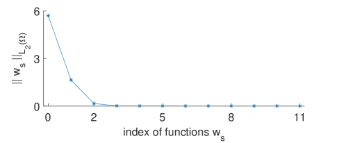
First, we select . To do this, we solve the forward problem (2.10), (2.18) for the case when the functions and (6.3) and (6.4) respectively and in Hence, by (6.5) the inclusion/background contrast is 2:1 in this case. Next, we calculate norms and compare them. We have observed that the norm of the function decreases very rapidly when the number is growing. More precisely, we have obtained that
| (6.11) |
which means less than 1%. The values of norms for are displayed in Table 1 and Figure 1. One can observe that starting from , these norms are much less than those for We conclude therefore, that we should take in our tests
| (6.12) |
| 0 | 1 | 2 | 3 | 4 | 5 | |
| 5.7122 | 1.6383 | 0.1630 | 0.0118 | 0.0091 | 0.0077 | |
| 6 | 7 | 8 | 9 | 10 | 11 | |
| 0.0067 | 0.0061 | 0.0055 | 0.0057 | 0.0058 | 0.0054 |
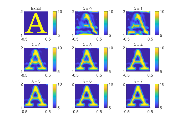
Next, given the optimal value of in (6.12), we select the optimal value of the parameter of the Carleman Weight Function in (6.8). To do this, we test the same letter ‘A’ with inside of it for values of the parameter Our numerical results are presented on Figure 2. We observe that the images have a low quality for Then the quality is improved and is stabilized at Thus, we treat as the optimal value of this parameter. We use this value in all subsequent tests. The value tells us that even though our theorems 4.1-4.5 require sufficiently large values of the parameter the computational practice shows that a reasonable value of can be chosen. The same observation was made in all previous works on the convexification of this research group, see items 2 and 3 in Remarks 4.1 in the end of section 4.
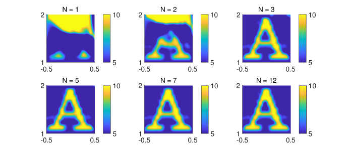
Now we want to demonstrate numerically again that is indeed a good choice of for our optimal value of Taking we test the same letter ‘A’ as above with in it, but for The results are displayed in Figure 3. One can observe that reconstructions have a low quality for . Next, the reconstructions are basically the same for However, the computational cost increases very rapidly with the increase of . Thus, using also Table 1, Figure 1 and (6.12), we conclude that to balance between the reconstruction accuracy and the computational cost, we should use . Thus, in all subsequent computations we use
| (6.13) |
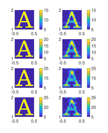
Test 2. We test the reconstruction of the coefficient with the shape of the letter ‘A’ where the function is given in (6.4) with different values of the parameter inside of the letter ‘A’. Thus, by (6.6) the inclusion/background contrasts now are respectively , and . Our computational results for this test are displayed on Figure 4. One can observe that the quality of these images is good for all four cases, although it slightly deteriorates for and The computed inclusion/background contrast is accurate, see (6.6).
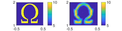
Test 3. We test the reconstruction of the coefficient with the shape of the letter ‘’ where the function is given in (6.4) with inside of the letter ‘’. Results are presented on Figure 5. We again observe an accurate reconstruction.
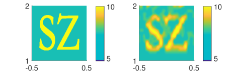
Test 4. We test the reconstruction of the coefficient with the shape of two letters ‘SZ’ where the function is given in (6.4) with inside of each of these two letters and outside of each of these two letters. In this test, as in (6.13). Results are presented on Figure 6. The image quality is lower than one for the case of the single letter ‘’ on Figure 5. Nevertheless, the quality is still good and the computed inclusion/background contrasts (6.6) are accurate in both letters.
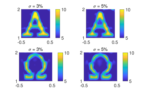
Test 5. In this test we use noisy data as in (6.9) with and i.e. with 3% and 5% noise level. We test the reconstruction of the coefficient with the shape of either the letter ‘A’ or the letter ‘’, where the function is given in (6.4) with inside of each of these two letters. Again, , as in (6.13). The results are shown in Figure 7. One can observe accurate reconstructions in all four cases. In particular, the inclusion/background contrasts (6.6) are reconstructed accurately.
References
- [1] A. B. Bakushinskii, M. V. Klibanov, and N. A. Koshev, Carleman weight functions for a globally convergent numerical method for ill-posed Cauchy problems for some quasilinear PDEs, Nonlinear Analysis: Real World Applications 34 (2017), 201–224.
- [2] G. Bal and A. Jollivet, Generalized stability estimates in inverse transport theory, Inverse Problems and Imaging 12 (2018), 59–90.
- [3] L. Baudouin, M. de Buhan, and S. Ervedoza, Convergent algorithm based on Carleman estimates for the recovery of a potential in the wave equation, SIAM J. Numerical Analysis 55 (2017), 1578–1613.
- [4] L. Baudouin, M. de Buhan, S. Ervedoza, and A. Osses, Carleman-based reconstruction algorithm for the waves, SIAM Journal on Numerical Analysis 59 (2021), 998–1039.
- [5] M. Bellassoued and M. Yamamoto, Carleman estimates and applications to inverse problems for hyperbolic systems, Springer, Japan, 2017.
- [6] M. Born and E. Wolf, Principles of optics, 7th ed., Cambridge University Press, 1999.
- [7] M Boulakia, M. de Buhan, and E. Schwindt, Numerical reconstruction based on Carleman estimates of a source term in a reaction-diffusion equation, ESAIM: Control, Optimisation and Calculus of Variations 27 (2021), S27, 1–34.
- [8] A. L. Bukhgeim and M. V. Klibanov, Uniqueness in the large of a class of multidimensional inverse problems, Soviet Math. Doklady 17 (1981), 244–247.
- [9] G. Chavent, Nonlinear Least Squares for Inverse Problems: Theoretical Foundations and Step-by-Step Guide for Applications, Springer Science & Business Media, Berlin, 2010.
- [10] B. B. Das, Feng Liu and R. R. Alfano, Time-resolved fluorescence and photon migration studies in biomedical and model random media, Rep. Prog. Phys. 60 (1997) 227–292.
- [11] H. Fujiwara, K. Sadiq, and A. Tamasan, A Fourier approach to the inverse source problem in an absorbing and anisotropic scattering medium, Inverse Problems 36 (2020), 015005.
- [12] H. Fujiwara, K. Sadiq, and A. Tamasan, Numerical reconstruction of radiative sources in an absorbing and nondiffusing scattering medium in two dimensions, SIAM J. Imaging Sciences 13 (2020), 535–555.
- [13] H. Fujiwara, K. Sadiq, and A. Tamasan, A source reconstrution method in two dimensional radiative transport using boundary data measured on an arc, Inverse Problems 37 (2021), 115005.
- [14] F. Gölgeleyen and M. Yamamoto, Stability for some inverse problems for transport equations, SIAM J. Mathematical Analysis 48 (2016), 2319–2344.
- [15] A. V. Goncharsky and S. Y. Romanov, A method of solving the coefficient inverse problems of wave tomography, Computers and Mathematics with Applications 77 (2019), 967–980.
- [16] J.P. Guillement and R. G. Novikov, Inversion of weighted Radon transforms via finite Fourier series weight approximation, Inverse Problems in Science and Engineering 22 (2013), 787–802.
- [17] J. Heino, S. Arridge, J. Sikora, and E. Somersalo, Anisotropic effects in highly scattering media, Physical Review E 68 (2003), 03198.
- [18] S. I. Kabanikhin, K. K. Sabelfeld, N. S. Novikov, and M. A. Shishlenin, Numerical solution of the multidimensional Gelfand-Levitan equation, J. Inverse and Ill-Posed Problems 23 (2015), 439–450.
- [19] V. A. Khoa, G. W. Bidney, M. V. Klibanov, L. H. Nguyen, A. Sullivan, L. Nguyen, and V. N. Astratov, Convexification and experimental data for a 3D inverse scattering problem with the moving point source, Inverse Problems 36 (2020), 085007.
- [20] M. V. Klibanov, Global convexity in a three-dimensional inverse acoustic problem, SIAM J. Math. Anal. 28 (1997), 1371–1388.
- [21] M. V. Klibanov and S.E. Pamyatnykh, Global uniqueness for a coefficient inverse problem for the non-stationary transport equation via Carleman estimate, J. Mathematical Analysis and Applications 343 (2008), 352–365.
- [22] M. V. Klibanov, Carleman estimates for global uniqueness, stability and numerical methods for coefficient inverse problems, J. Inverse and Ill-Posed Problems 21 (2013), 477–510.
- [23] M. V. Klibanov, Convexification of restricted Dirichlet to Neumann map, J. Inverse and Ill-Posed Problems 25 (2017), no. 5, 669–685.
- [24] M. V. Klibanov and O. V. Ioussoupova, Uniform strict convexity of a cost functional for three-dimensional inverse scattering problem, SIAM J. Math. Anal 26 (1995), 147–179.
- [25] M. V. Klibanov, V. A. Khoa, A. V. Smirnov, L. H. Nguyen, G. W. Bidney, L. Nguyen, A. Sullivan, and V. N. Astratov, Convexification inversion method for nonlinear SAR imaging with experimentally collected data, Journal of Applied and Industrial Mathematics 15 (2021), 413–436.
- [26] M. V. Klibanov and J. Li, Inverse Problems and Carleman Estimates: Global Uniqueness, Global Convergence and Experimental Data, De Gruyter, 2021.
- [27] M. V. Klibanov, J. Li, and W. Zhang, Electrical impedance tomography with restricted dirichlet-to-neumann map data, Inverse Problems 35 (2019), 35005.
- [28] R.Y. Lay and Q. Li, Parameter reconstruction for general transport equation, SIAM J. Mathematical Analysis 52 (2020), 2734–2758.
- [29] F. Natterer, The Mathematics of Computerized Tomography, SIAM publications, 2001.
- [30] R. G. Novikov, An inversion formula for the attenuated X-ray transformation, Ark. Mat. 40 (2002), 145–167.
- [31] A. V. Smirnov, M. V. Klibanov, and L. H. Nguyen, On an inverse source problem for the full radiative transfer equation with incomplete data, SIAM J. Scientific Computing 41 (2019), B929–B952.
- [32] P. Stefanov and G. Uhlmann, An inverse source problem in optical molecular imaging, Analysis and PDE 1 (2008), 115–126.
- [33] A. N. Tikhonov, A. V. Goncharsky, V. V. Stepanov, and A. G. Yagola, Numerical methods for the solution of ill-posed problems, Kluwer, London, 1995.
- [34] M. M. Vajnberg, Variational method and method of monotone operators in the theory of nonlinear equations, Israel Program for Scientific Translations, Jerusalem-London, 1973.