Lemma 2.

$O(\frac{2\log(2/\delta)}{\epsilon^{2}})$ measurements suffice to bound the error from a Hadamard test to be within $\epsilon$ with probability $1-\delta$.

Proof: Assume $m$ measurements are performed on the control bit of the Hadamard test with outcomes $M_{1},M_{2},...,M_{m}\in\{0,1\}$, we can approximate $\Pr(1)$ using $\widehat{\Pr(1)}=\frac{1}{m}\sum_{i=1}^{m}M_{i}$. Applying the Chernoff-Hoeffding bound, P ( —(1-2^Pr(1)) - (1-2Pr(1))—¿ϵ) =P ( —^Pr(1)- Pr(1)—¿ϵ2 ) ¡ 2e^-ϵ^2m/2. When $m\geq\frac{2\log(2/\delta)}{\epsilon^{2}}$, $2e^{-{\epsilon^{2}}m/2}\leq\delta$, and this completes the proof.

Lemma 3.

Given an arbitrary pure state $\ket{x}\in\partial B_{\mathbb{C}^{N}}(0,1)$ and a mixed quantum operation $\tilde{U}=\sum_{\kappa=1}^{K}\alpha_{\kappa}U_{\kappa}$ with $\sum_{\kappa=1}^{K}\absolutevalue{\alpha_{\kappa}}\leq 1$ and $K\sim O(1)$, $O(\frac{32K^{4}\log(4K^{2}/\delta)}{\epsilon^{2}})$ measurements suffice to estimate $\bra{x}\tilde{U}\tilde{U}^{\dagger}\ket{x}$ to an error within $\epsilon$ with probability at least $1-\delta$.

Proof: According to equation (LABEL:eq2), $\bra{x}\tilde{U}\tilde{U}^{\dagger}\ket{x}$ can be estimated with a summation of $O(2K^{2})$ measurements from the Hadamard tests. By the assumption $\sum_{\kappa=1}^{K}\absolutevalue{\alpha_{\kappa}}\leq 1$, $2\real\{\alpha_{\kappa_{1}}\alpha^{*}_{\kappa 2}\}$ and $2\imaginary\{\alpha_{\kappa_{1}}\alpha^{*}_{\kappa 2}\}$ are both $\leq 2$. Applying the triangle inequality and the union bound, it suffices to bound the error of each Hadamard test to be within $\frac{\epsilon}{4K^{2}}$ with probability at least $1-\frac{\delta}{2K^{2}}$. We then apply Lemma 2 and obtain an upper bound on the sample complexity, $m=O(\frac{32K^{4}\log(4K^{2}/\delta)}{\epsilon^{2}})$. With the assumption $K\sim O(1)$, Lemma 3 implies a low-order polynomial measurement complexity to estimate the measurement outcome of the Hadamard test to a marginal error. Thus, we make an assumption that all measurements are error-free from now on.

For an arbitrary mixed quantum operation $\tilde{U}$, we can approximate $\tilde{\norm{U}}_{S_{2}}$ using $m$ random samples. Namely, we randomly sample $\theta_{1},...,\theta_{m}\sim\mathcal{D}=\text{Uni}[-\pi,\pi]$ and use the sampling circuit $S$ as defined by (LABEL:Sdef) to approximate

$$\widehat{\tilde{\norm{U}}}_{S_{2}}=\sqrt{\frac{1}{m}\sum_{i=1}^{m}\bra{\boldsymbol{0}}S^{\dagger}(\theta_{i})\tilde{U}\tilde{U}^{\dagger}S(\theta_{i})\ket{\boldsymbol{0}}}$$ (6)

where each $\bra{\boldsymbol{0}}S^{\dagger}(\theta_{i})\tilde{U}\tilde{U}^{\dagger}S(\theta_{i})\ket{\boldsymbol{0}}$ can be measured with negligible error by Lemma 3.

Theorem 3.

For an arbitrary mixed quantum operation $\tilde{U}$, we can estimate its normalized Schatten 2-norm efficiently using quantum sampling circuits of depth overhead $O(1)$. Moreover, for any $\delta$, $\epsilon>0$, with sample complexity $m(\epsilon,\delta)=O(\frac{\log(2/\delta)}{2\epsilon^{2}}\min\{\epsilon^{-2},\tilde{\norm{U}}_{S_{2}}^{-2}\})$, samples $\theta_{1},...,\theta_{m(\epsilon,\delta)}\sim\text{Uni}[-\pi,\pi]$, and $S(\theta_{i})$ as defined by (LABEL:Sdef), the following holds for the quantum approximation of $\tilde{\norm{{U}}}_{S_{2}}$ using (6). P(—^~∥U∥_S_2 - ~∥U∥_S_2—¡ ϵ) ¿ 1-δ.

Proof: The Theorem follows from Theorem LABEL:theorem2, Table LABEL:measurement_ckt, and Lemma 3. Note that the sample complexity for the approximation of the normalized Schatten 2-norm is independent of the number of qubits and is polynomial to $\frac{1}{\epsilon}$, which implies a potential quantum advantage. In Figure 2, we present simulated results supporting the relation $\epsilon\propto m(\epsilon,\delta)^{-1/2}$ which is in agreement with Theorem 3.

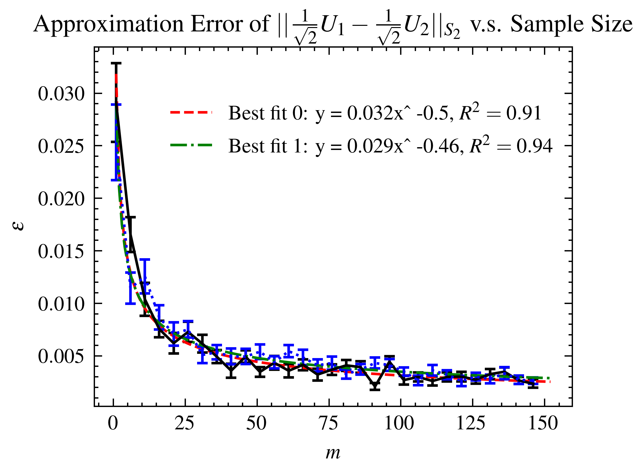
Figure 2: For each randomly generated mixed quantum operations $\tilde{U}=\frac{1}{\sqrt{2}}U_{1}-\frac{1}{\sqrt{2}}U_{2}$ where $U_{1}$, $U_{2}$ are randomly generated using the QR decomposition https://doi.org/10.48550/arxiv.math-ph/0609050, we plot the error of the approximation $\widehat{\tilde{\norm{U}}}_{S_{2}}$ with respect to the sample size $m$ as defined in Theorem 3. A 6-qubit system is considered. The means and standard errors are computed over 30 sets of random samples.

In the next section, we build a connection from the normalized Schatten 2-norm of the difference of quantum operations to the similarity metric defined in Section LABEL:background.

5 From the Normalized Schatten 2-Norm to a Fidelity-based Similarity Metric

Recall the definition of pure-state $(\epsilon,\delta)$-similarity. Let $\ket{\psi}$ be a random state sampled from the distribution $\mathcal{J}=\text{Uni}[\partial B_{\mathbb{C}^{N}}(0,1)]$, we define two unitary operations $U_{1}$, $U_{2}$ to be pure-state $(\delta,\epsilon)$-similar if

$$\mathbb{P}_{\psi\sim\mathcal{J}}(\mathcal{F}(U_{1}\ket{\psi},U_{2}\ket{\psi})\geq 1-\epsilon) \geq 1-\delta.$$

The following lemma is significant as it relates pure-state $(\epsilon,\delta)$-similarity to the normalized Schatten 2-norm.

Lemma 4.

Let ${U}_{1},U_{2}$ be two unitary quantum operations. ${U}_{1}$, ${U}_{2}$ are pure-state $(\epsilon,\delta)$-similar if $\norm{U_{1}-U_{2}}_{S_{2}}\leq\frac{\epsilon}{1+\sqrt{2(1/\delta-1)}}$.

Proof: We apply statistical analysis to study the expectation and the variance of $\mathcal{F}(U_{1}\ket{\psi},U_{2}\ket{\psi})$ when $\ket{\psi}\sim\mathcal{J}=\text{Uni}[\partial B_{\mathbb{C}^{N}}(0,1)]$. For any pure state $\ket{\psi}$,

$$\mathcal{F}(U_{1}\ket{\psi},U_{2}\ket{\psi})=\absolutevalue{\bra{\psi}U_{1}^{\dagger}U_{2}\ket{\psi}}^{2}\geq\real^{2}\{\bra{\psi}U_{1}^{\dagger}U_{2}\ket{\psi}\}\\ =(1-\frac{\sum_{i=1}^{N}{\sigma_{i}}^{2}\absolutevalue{\bra{w_{i}}\ket{\psi}}^{2}}{2})^{2}\geq 1-\sum_{i=1}^{N}{\sigma_{i}}^{2}\absolutevalue{\bra{w_{i}}\ket{\psi}}^{2},$$

where $w_{i}$ and $\sigma_{i}$ are the left-singular vectors and singular values of $U_{1}-U_{2}$. Let $\hat{\epsilon}=\norm{U_{1}-U_{2}}_{S_{2}}$ and $\ket{\psi}\sim\mathcal{J}$, E_—ψ⟩∼JF(U_1—ψ⟩, U_2—ψ⟩) ≥1-∥U_1-U_2∥_S_2^2 ≥1-^ϵ^2. We next compute the variance of the fidelity,

$$\text{Var}_{\ket{\psi}\sim\mathcal{J}}[\mathcal{F}(U_{1}\ket{\psi},U_{2}\ket{\psi})] =\operatorname{\mathbb{E}}_{\ket{\psi}}\mathcal{F}^{2}(U_{1}\ket{\psi},U_{2}\ket{\psi})-\big{(}\operatorname{\mathbb{E}}_{\ket{\psi}}\mathcal{F}(U_{1}\ket{\psi},U_{2}\ket{\psi})\big{)}^{2}$$

$$\leq 1-(1-\hat{\epsilon}^{2})^{2}\leq 2\hat{\epsilon}^{2}.$$

Application of the Chebyshev-Cantelli inequality, for arbitrary $c>0$, P_—ψ⟩∼J(F(U_1—ψ⟩, U_2—ψ⟩) ≥1-c)≥1-2^ϵ2(c-^ϵ2)2+2^ϵ2. Setting $c=\epsilon$ and $\frac{2\hat{\epsilon}^{2}}{(c-\hat{\epsilon}^{2})^{2}+2\hat{\epsilon}^{2}}=\delta$, it suffices to have $\hat{\epsilon}\leq\frac{\epsilon}{1+\sqrt{2(1/\delta-1)}}$. Empirical relations between $\mathcal{F}(U_{1}\ket{\psi},U_{2}\ket{\psi})$ and $\norm{U_{1}-U_{2}}_{S_{2}}$ are illustrated in Figures 3 and 4. In both experiments, $U_{1}$ is a fixed random unitary generated by QR decomposition https://doi.org/10.48550/arxiv.math-ph/0609050 and $U_{2}$ is constructed by applying rotation operators to $U_{1}$. Figure 4 supports the bound derived in Lemma 4 as the probability for $U_{1}$, $U_{2}$ to be pure-state $\big{(}(1+\sqrt{8})\norm{U_{1}-U_{2}}_{S_{2}},0.2\big{)}$-similar is much higher than $0.8$ for all pairs of $U_{1}$ and $U_{2}$ used (setting $\delta=0.2$).

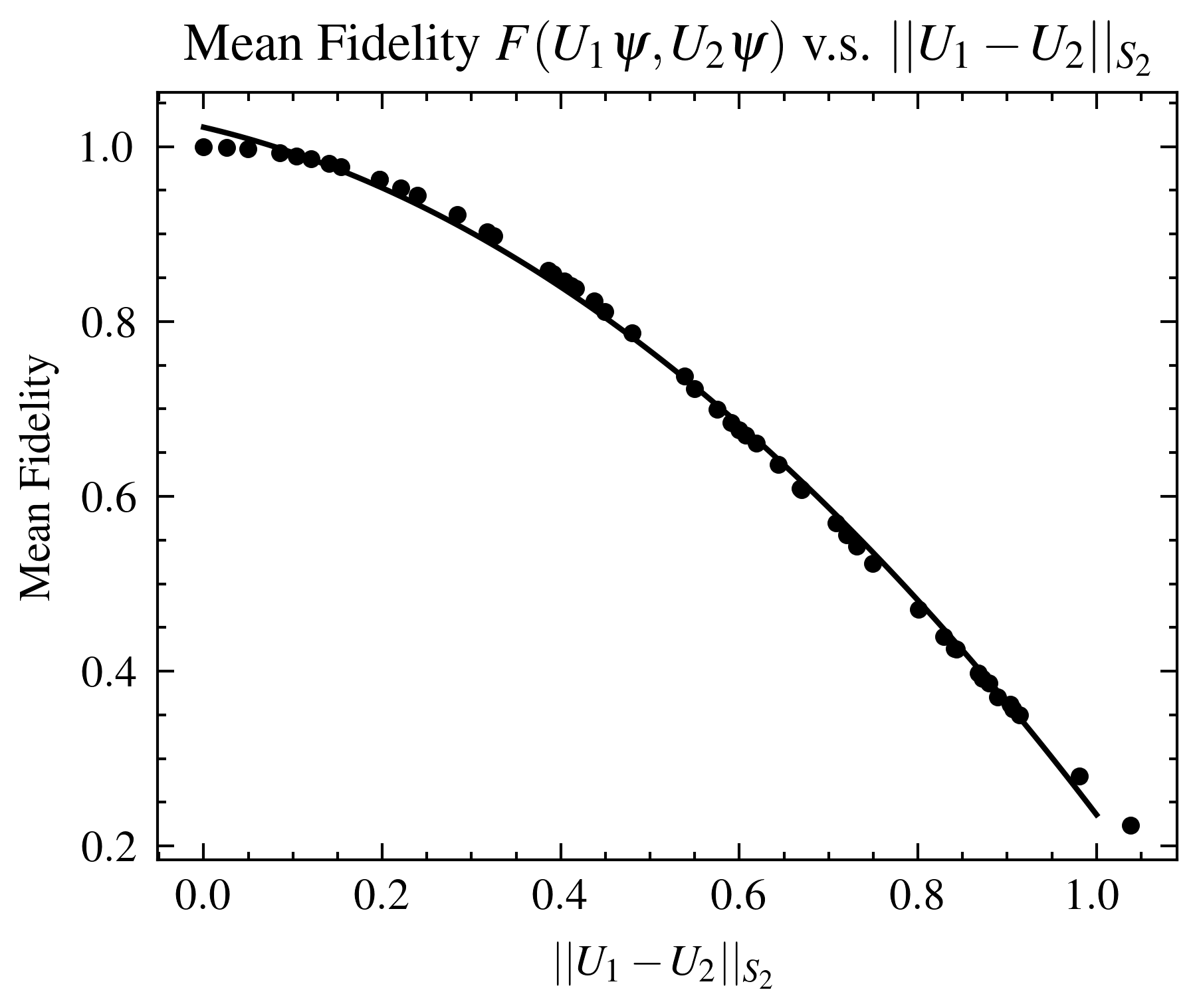
Figure 3: Empirical relation between approximated $\operatorname{\mathbb{E}}_{\psi\sim\text{Uni}[\partial B_{\mathbb{C}^{N}}(0,1)]}\mathcal{F}(U_{1}\ket{\psi},U_{2}\ket{\psi})$ and $\norm{U_{1}-U_{2}}_{S_{2}}$. For each pair of $U_{1}$ and $U_{2}$, the mean fidelity is computed over 1000 randomly sampled (with replacement) states $\psi\sim\text{Uni}[\partial B_{\mathbb{C}^{N}}(0,1)]$. A 6-qubit system is considered.

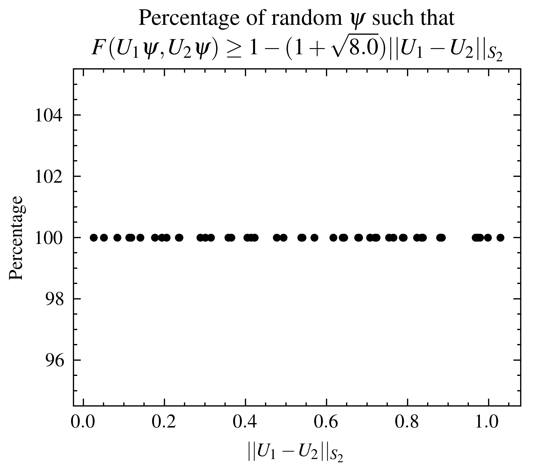
Figure 4: Verification of Lemma 4 when $\delta=0.2$. For each pair of $U_{1}$ and $U_{2}$, the percentage is computed over 1000 randomly sampled (with replacement) $\psi\sim\text{Uni}[\partial B_{\mathbb{C}^{N}}(0,1)]$. A 6-qubit system is considered.

The lemma can be generalized to mixed quantum operations. Let $\mathcal{J}=\text{Uni}[\partial B_{\mathbb{C}^{N}}(0,1)]$, we define two mixed quantum operations $\tilde{U}_{1},\tilde{U}_{2}$ to be pure-state $(\epsilon,\delta)$-similar if P_—ψ⟩∼J(F(~U_1—ψ⟩, ~U_2—ψ⟩)≥E_ψ^2⟨ψ—~U1~U1†+ ~U2~U2†—ψ⟩2-ϵ)≥1-δ.

Lemma 5.

Let $\tilde{U}_{1},\tilde{U}_{2}$ be two mixed quantum operations and $\mathcal{J}=\text{Uni}[\partial B_{\mathbb{C}^{N}}(0,1)]$. $\tilde{U}_{1}$, $\tilde{U}_{2}$ are pure-state $(\epsilon,\delta)$-similar if $\norm{\tilde{U}_{1}-\tilde{U}_{2}}_{S_{2}}\leq\sqrt{\frac{\epsilon^{2}-(1/\delta-1)(\tau-\tau^{4})}{2\tau(\epsilon+(1/\delta-1)\tau^{2})}}$, where $\tau=\operatorname{\mathbb{E}}_{\ket{\psi}\sim\mathcal{J}}\frac{\bra{\psi}\tilde{U}_{1}\tilde{U}_{1}^{\dagger}+\tilde{U}_{2}\tilde{U}_{2}^{\dagger}\ket{\psi}}{2}$.

Proof: For any given pure state $\ket{\psi}\in\partial B_{\mathbb{C}^{N}}(0,1)$,

$$\mathcal{F}(\tilde{U}_{1}\ket{\psi},\tilde{U}_{2}\ket{\psi}) \geq\real^{2}\{\bra{\psi}\tilde{U}_{1}^{\dagger}\tilde{U}_{2}\ket{\psi}\}$$

$$=(\frac{\bra{\psi}\tilde{U}_{1}\tilde{U}_{1}^{\dagger}\ket{\psi}+\bra{\psi}\tilde{U}_{2}\tilde{U}_{2}^{\dagger}\ket{\psi}}{2}-\frac{\sum_{i=1}^{N}{\sigma_{i}}^{2}\absolutevalue{\bra{w_{i}}\ket{\psi}}^{2}}{2})^{2},$$

where $w_{i}$ and $\sigma_{i}$ are the left-singular vectors and singular values of $\tilde{U}_{1}-\tilde{U}_{2}$. Let $\tau=\operatorname{\mathbb{E}}_{\ket{\psi}\sim\mathcal{J}}\frac{\bra{\psi}\tilde{U}_{1}\tilde{U}_{1}^{\dagger}\ket{\psi}+\bra{\psi}\tilde{U}_{2}\tilde{U}_{2}^{\dagger}\ket{\psi}}{2}$ and $\hat{\epsilon}=\norm{\tilde{U}_{1}-\tilde{U}_{2}}_{S_{2}}$, E_—ψ⟩ ∼J F(~U_1—ψ⟩, ~U