Evolutionary Time-Use Optimization for Improving Children’s Health Outcomes

Abstract

How someone allocates their time is important to their health and well-being. In this paper, we show how evolutionary algorithms can be used to promote health and well-being by optimizing time usage. Based on data from a large population-based child cohort, we design fitness functions to explain health outcomes and introduce constraints for viable time plans. We then investigate the performance of evolutionary algorithms to optimize time use for four individual health outcomes with hypothetical children with different day structures. As the four health outcomes are competing for time allocations, we study how to optimize multiple health outcomes simultaneously in the form of a multi-objective optimization problem. We optimize one-week time-use plans using evolutionary multi-objective algorithms and point out the trade-offs achievable with respect to different health outcomes.

Keywords Real-world application  $\cdot$ time-use optimization  $\cdot$ single-objective optimization  $\cdot$ multi-objective optimization.

1 Introduction

Evolutionary algorithms (EAs) are bio-inspired randomized optimization techniques and have been very successfully applied to various real-world combinatorial optimization problems [20, 24, 28]. Evolutionary algorithms use a population of search points in the decision space of a given optimization problem to solve the problem. Moreover, many real-world optimization problems consist of several conflicting objectives that must be optimized simultaneously. No single solution can optimize multiple objectives, instead a set of trade-off optimal solutions is obtained. EAs can approximate multiple optimal solutions in a single run, which make EAs popular in solving multi-objective optimization problems [11, 14].

A real-world multi-objective optimization problem is "How should children spend their time (i.e. sleeping, sedentary behaviour and physical activity) to optimize their health, well-being, and cognitive development?" [9, 8]. The importance of this problem has led governing bodies and health authorities such as the World Health Organization (WHO) to provide guidelines for daily durations of sleep, screen time, and physical activity [31]. Such guidelines for school-aged children (5-12 years) currently recommend 9-11 hours of sleep, no more than 2 hours of sedentary screen time, and at least 1 hour of moderate-to-vigorous physical activity (MVPA) per day [31]. However, these guidelines are primarily underpinned by systematic reviews collating evidence of how the duration of a single behaviour, such as MVPA, is associated with a single measure of health or wellbeing [31]. These studies show whether more or less of behaviour is beneficially associated with the outcome [8, 9, 31], rather than identifying optimal durations, which would be required to support recommendations for daily durations of the behaviour. Almost no studies have attempted to define optimal durations for these activity behaviours for a single health outcome, let alone for multiple health and well-being outcomes.

To address the lack of evidence for optimal time-use allocations, a recent study [16] used compositional linear regression [17] to model the relationship between how children allocated their daily time to four activities (sleep, sedentary behaviour, light physical activity (LPA) and MVPA) and twelve outcomes spanning physical, mental and cognitive health domains. Compositional data analysis enabled all four activities to be included in a single model whilst ensuring their constant-sum constraint to 24 hours was respected [1]. Using published compositional data methods, the raw activity data of minutes per day were expressed as a set of isometric log-ratios [29]. With these compositional regression models, [18] estimated values of the outcomes for every possible and feasible combination of sleep, sedentary behaviour, LPA and MVPA duration were calculated. Optimal daily duration of the activities were derived for each of the twelve health outcomes from the average “time-use composition” associated with the best $5\%$ of estimated values for the respective health outcomes.

It remains unknown how to perform the best multi-objective optimisation of time use for overall health and well-being. The method developed by [18] is computationally intensive for four activities requiring almost 4 million iterations of different possible time-use scenarios. This method becomes unfeasible with a large number of daily activities (e.g., activities such as chores, sport, transport, school, sleep, quiet time, social time, screen time, etc.) routinely collected by time-use recalls [34]. Additionally, varying constraints to daily time use, which may limit application to the real world, were not considered.

The research described in this paper extends previous work proposed in [16] by considering four decision variables: daily time allocation to sleep, sedentary behaviour, LPA and MVPA, and four health objectives for children: body mass index (BMI), cognition, life satisfaction and fitness. Firstly, we formulate the one-day time-use optimization problem as a single-objective problem in continuous space by optimizing one of the four presented health outcomes. Then, we extend the one-day time-use schedule to one week and present multi-objective optimization models for the time-use optimization problem.

EAs are introduced to develop time-use optimization approaches that incorporate daily and weekly time constraint schedules and provide decision-making tools for trading off multiple health outcomes against each other. For single-objective time-use optimization, we evaluate the performance of the differential evolution (DE) algorithm [37] with different operators, particle swarm optimization (PSO) [25] and covariance matrix adaptation evolutionary strategy (CMA-ES)[22, 21] to optimize health outcomes in different day structures. For multi-objective time-use optimization, we investigate the performance of the multi-objective evolutionary algorithm based on decomposition (MOEA/D) [41], Non-dominated sorting genetic algorithm (NSGA-II) [15] and Strong Pareto evolutionary algorithm 2 (SPEA2) [43].

The paper is organized as follows. We introduce the data set used in Section 1.1. Section 2 describes application of our time-use optimization models for different health outcomes, and to different day constraints. The proposed optimization methods are described in Section 3. The results of the optimization experiments are described in Section 4. Conclusions and avenues for future work are presented in Section 5.

1.1 Data Description

This study uses data from a large population-based child cohort to illustrate the real-world application of a novel time-use optimisation procedure. Data were from the Child Health CheckPoint study [10], a cross-sectional module nested between waves 6 and 7 of the Longitudinal Study of Australian Children (LSAC) [19]. Child participants of the LSAC birth cohort (commenced in 2004 with n=5107) that were retained to Wave 6 $(n=3764)$ were invited to take part in Child Health CheckPoint (2015-16) when they were 11-12 years old. Of these, $n=1874$ $(50\%)$ consented to participate via written informed consent from their parent/guardian. Ethical approval for CheckPoint was granted by The Royal Children’s Hospital (Melbourne) Human Research Ethics Committee (HREC33225D) and the Australian Institute of Family Studies Ethics Committee (AIFS14-26).

Participants were fitted with a wrist-worn accelerometer (GENEActive, Activinsights Ltd, UK) by a trained researcher, with instructions to wear the device 24 hours a day for eight days. Following the return of the device, activity data were downloaded and processed following published procedures [16, 19] to determine the average daily minutes spent in sleep, sedentary time, LPA and MVPA.

BMI was derived from the child participant’s measured height (Invicta 10955 stadiometer) and weight (2-limb Tanita BC-351 or 4-limb InBody 230). BMI was calculated as weight (kg)/height $(m)^{2}$ and expressed as age- and sex-specific z-scores [32]. The cognition score was derived from the NIH Picture Vocab test, which asks the child to select on an iPad a picture that best represents the meaning of words they hear through headphones [40]. A higher score indicates better receptive vocabulary, which represents cognition. Life satisfaction was obtained from the 5-item Brief Multi-Dimensional Students’ Life Satisfaction Scale, with a higher score indicating higher satisfaction with their family life, friendships, school experience and themselves, where they live, and their overall life [36]. Fitness was obtained from a cycle ergometer test which was used to determine the estimated maximal work rate from which VO2max (predicted maximal aerobic power) was estimated. A higher VO2max indicates better aerobic fitness [6].

2 The Time-Use Optimization Models

In this section, we first list the notations and descriptions of health outcomes and decision variables in Table 1(a). Column Optimal lists the definition of optimal value of each objective. Then, we introduce a general model for the one-day time-use optimization problem without considering any specific day structure or health outcome.

obj: $$f(x)=\hat{\beta_{0}}+\hat{\beta_{1}}z_{1}+\hat{\beta_{2}}z_{2}+\hat{\beta_{3}}z_{3}+\hat{\beta_{4}}z_{1}z_{1}+\hat{\beta_{5}}z_{1}z_{2}$$

$$+\hat{\beta_{6}}z_{1}z_{3}+\hat{\beta_{7}}z_{2}z_{2}+\hat{\beta_{8}}z_{2}z_{3}+\hat{\beta_{9}}z_{3}z_{3}$$ (1)

s.t. $$z_{1}=\sqrt{\frac{3}{4}}\ln\left(\frac{x_{1}}{\sqrt[3]{x_{2}x_{3}x_{4}}}\right),z_{2}=\sqrt{\frac{2}{3}}\ln\left(\frac{x_{2}}{\sqrt{x_{3}x_{4}}}\right),z_{3}=\sqrt{\frac{1}{2}}\ln\left(\frac{x_{3}}{x_{4}}\right)$$

$$\sum_{i=1}^{4}x_{i}=1440$$ (2)

$$x_{i}^{l}\leq x_{i}\leq x_{i}^{u}\quad\forall i=\{1,\ldots,4\}$$ (3)

The decision vector of this model can be expressed as $x=\{x_{1},x_{2},x_{3},x_{4}\}$ which consists of four activity variables (sleep, sedentary time, LPA, MVPA). The objective function (1) shows how to calculate health outcomes based on values of the decision variables and parameters. Where $\beta_{0},\beta_{1},\ldots,\beta_{9}$ are unknown regression coefficients to be estimated, they are different in the objective function of each health outcome. Here, those regression coefficients are estimated using the data described in Section 1.1. We list the estimated values $\hat{\beta_{i}},i=\{1,\ldots,9\}$ for different health outcomes in Table 1 (b) and introduce how to obtain those values in Section 2.1. Constraint (2) forces the sum of decision variables of the problem equal to the total minutes (1440 min) per day. We introduce a closure operation (see Algorithm 1) to tackle this constraint and make the working progress of any search algorithm fast to achieve a feasible solution. Upper and lower bounds on each decision variables are enforced by constraint (3), where $x_{i}^{l}$ denotes the lower bound of $x_{i}$ and $x_{i}^{u}$ denotes the upper bound of $x_{i}$. The upper and lower bounds are different according to the day structure considered.

Without loss of generality, we study six different hypothetical day structures. We label these day structures to reflect real-world scenarios: Studious day (STD), Sporty day (SPD), After-School Job day (ASJD), Sporty Weekend day (SPWD), Studious/screen weekend day (STWD) and Working weekend day (WWD). The lower and upper bounds of the decision variables are set to suit the day-above-day structures, as advised by an external child behavioural epidemiologist, and by considering the empirical activity durations found in the underlying data (please refer to Table 2). These replace the 24-hour constraint (3) which is present in a general model.

Table 1: Notation and values of parameters

(a) Description of notation			(b) Estimated regression coefficients
Notation	Description	Optimal	Notation	$f_{1}$	$f_{2}$	$f_{3}$	$f_{4}$
$f_{1}$	Body mass index (BMI)	$\min|f_{1}|$	$\beta_{0}$	0.23307	2.3508268	12395.053	68.85903
$f_{2}$	Cognition (vocab) objective	$\max f_{2}$	$\beta_{1}$	-0.59691	-0.032037	2255.008	-17.84326
$f_{3}$	Life satisfaction objective	$\max f_{3}$	$\beta_{2}$	0.05029	0.0670568	-885.351	-1.77607
$f_{4}$	Fitness (VO2max) objective	$\max f_{4}$	$\beta_{3}$	0.68497	-0.003155	-1264.635	-11.25996
			$\beta_{4}$	0	0	0	3.15694
$x_{1}$	Minutes of sleeping		$\beta_{5}$	0	0	0	13.88458
$x_{2}$	Minutes of sedentary behaviour		$\beta_{6}$	0	0	0	-5.12788
$x_{3}$	Minutes of LPA		$\beta_{7}$	0	0	0	-6.85649
$x_{4}$	Minutes of MVPA		$\beta_{8}$	0	0	0	2.69689
			$\beta_{9}$	0	0	0	2.52276

Table 2: Values of lower bounds and upper bounds

		Studious	Sporty	After-school	Sporty	Studious/screen	Working
		day	day	job day	weekend day	weekend day	weekend day
Sleep	LB	360	360	360	420	420	360
	UB	720	720	720	720	720	720
Sedentary	LB	690	480	480	210	270	210
	UB	900	900	900	900	900	900
LPA	LB	150	210	220	210	150	390
	UB	480	480	480	480	480	480
MVPA	LB	1	61	1	61	1	1
	UB	210	210	210	210	210	210

2.1 Model parameter estimation

Estimates of the model parameters ($\hat{\beta}_{i},i=1,\ldots,9$) in Equation (1) are calculated using least-squares multiple linear regression on the CheckPoint data. It is not possible to use all the untransformed time-use predictors simultaneously in the linear model as they are linearly dependent which in turn prohibits the matrix inverse calculation in estimating the parameter estimates. The isometric log ratio (ilr) transformation is a widely used transformation of the predictors to remove the linear dependence in the predictors [17].

For each outcome variable, $f_{1},f_{2},f_{3},f_{4}$, the Box-Cox transformation is applied after removing predictor effects for variance stabilisation, and improvement in the normality of the residuals [7]. Quadratic terms of the time-use ilr predictors are considered for each outcome model which correspond to the model terms associated with the parameters $\beta_{4},\ldots,\beta_{9}$ in Equation (1). If the quadratic terms do not significantly improve the model fit statistically at the $\alpha=0.05$ level (ANOVA $F$-test), the model parameters $\beta_{4},\ldots,\beta_{9}$ are set to 0 (i.e., only linear ilr terms remain). For more information about fitting quadratic compositional terms in linear regression, we refer to Chapter 5 of [38].

The full fit of the linear model also includes covariates of age, sex and puberty status and their associated coefficients. The sample average covariates are then used (age=12, female/male=1:1 and puberty status="Midpubertal"). The estimated effects of these covariates, and the intercept term of the model, are included as the $\beta_{0}$ term in Equation (1). The objective functions therefore become the prediction for the theoretical average child in the sample. A sample with missing values in either the outcome or the predictors is removed in each model fit as data are reasonably assumed to be missing at random [35]. Diagnostic plots of each model are observed to ensure the model assumptions are reasonable. All analysis is performed in R version 4.0.3 [33].

Input: Decision vector $\{x_{1},x_{2},x_{3},x_{4}\}$

$a=\sum_{i=1}^{4}x_{i}$;

for $i=1$ to $4$ do

       $x_{i}=\frac{1440x_{i}}{a}$;

      

return the decision variables.

Algorithm 1 Closure Operation

2.2 One Week Plan

We extend the one-day problem to a one-week problem by mixing different day structures, given seven days where each day has four decision variables $x_{d}=\{x_{d1},x_{d2},x_{d3},x_{d4}\}$. Different mixtures shown in Table 3 were used to make the one-week plans more realistic. The number listed in each column shows how many of each day type are planned for the week. The objective function for a one-week plan is $F(x)=\sum_{d=1}^{7}f(x_{d})$ which is subject to the constraints of each included day.

Table 3: Different mixture of one-week plan

Index	Studious	Sporty	After-school	Sporty	Studious/screen	Working
	day	day	job day	weekend day	weekend day	weekend day
1	3	1	0	1	1	1
2	3	0	2	0	1	1
3	3	2	0	0	1	1
4	2	2	1	0	2	0
5	2	2	0	1	0	2
6	2	2	1	1	1	0

2.3 Multi-objectives Problem

Now, we introduce a multi-objective model for time-use optimization. A multi-objective model involves finding solutions to optimize the problem defined by at least two conflicting objectives. The multi-objective model of time-use optimization can be defined as follows.

Objs: $$M(x)=[f_{1}(x),f_{2}(x),f_{3}(x),f_{4}(x)]$$ (4)

$$s.t.\quad \sum_{i=1}^{4}x_{i}=1440$$ (5)

$$x_{i}^{l}\leq x_{i}\leq x_{i}^{u}\quad\forall i=\{1,\ldots,4\}$$ (6)

where $x$ denotes a solution, $f_{i}(x)\rightarrow\mathbb{R}$ denotes the $i$th objective function to be optimized. Since there are four single objectives studied in this paper, we investigate all combinatorial objectives as multi-objective problems.

2.4 Fitness function

We investigate the performance of different evolutionary algorithms for single-objective and multi-objective time-use optimization problems. The fitness of a solution $x$ considers all constraints of one-day time-use optimization and one-week time-use optimization $h(x)$ and $H(x)$ separately.

$$h(x) =(u(x),f(x))$$ (7)

$$H(x) =(U(x),F(x)),$$ (8)

where $u(x)=\sum_{i=1}^{4}\max\{0,x_{i}-x_{i}^{u},x_{i}^{l}-x_{i}\}$ and $U(x)=\sum_{d=1}^{7}\sum_{i=1}^{4}\max\{0,x_{di}-x_{di}^{u},x_{di}^{l}-x_{di}\}$. We optimize $h$ and $H$ with respect to lexicographic order, i.e. $h(x)\geq h(y)$ holds iff $u(x)<u(y)\vee(u(x)=u(y)\wedge f(x)\geq f(y))$ for objective $f_{2}$, $f_{3}$ and $f_{4}$, $u(x)<u(y)\vee(u(x)=u(y)\wedge|f(x)|\leq|f(y)|)$ for objective $f_{1}$. Therefore, for the time-use optimization problem, any infeasible solution that violates the boundary constraints is worse than any feasible solution. Among solutions that meet all constraints, we aim to optimize the objective function.

3 Evolutionary Algorithms for the Time-Use Optimisation Problem

The algorithms that follow are classified into two classes. The first one contains single-objective evolutionary algorithms (Section 3.1), and the second has multi-objective evolutionary algorithms (Section 3.2). In this section, we only list the algorithms implemented in this study without detailed descriptions. Moreover, when implementing the presented algorithm for solving time-use optimization, Algorithm 1 is conducted before evaluating a generated solution.

3.1 Single-objective evolutionary algorithms

For the single-objective time-use optimization, we compare three evolutionary algorithms to optimize all health outcomes in different day structures.

Differential Evolution (DE)[13, 37] is a well known global search heuristic using a binomial crossover and a mutation operator. We evaluate two mutation operators DE/rand/1 and DE/current-to-rand/1 for the single-objective time -use optimization problem. The population size is set to $50$, and other control parameters are $F=0.5$, $C_{r}=0.5$.

Particle Swarm Optimization (PSO)[2, 27], is a type of swarm intelligence evolutionary algorithm, with population size $50$, $c_{1}=1$, $c_{2}=1$. For more understanding the working processes of PSO, we refer to [4, 5, 23, 26, 39, 42].

Covariance matrix adaptation evolutionary strategy (CMA-ES)[22, 21] is a self-adaptive evolution strategy that solves non-linear non-convex optimization problems in continuous domains. We implement the CMA-ES using $\lambda=10$ and $\sigma=0.3$.

3.2 Multi-objective evolutionary algorithms

For multi-objective time-use optimization, three multi-objective evolutionary algorithms are considered here.

Multi-objective evolutionary algorithm based on decomposition (MOEA/D) is a decomposition based algorithm commonly used to solve multi-objective optimisation problems [41]. We use the standard version of MOEA/D with the Tchebycheff approach, and population size is set to $100$.

Non-dominated sorting genetic algorithm (NSGA-II) [15] is a fast non-dominated sorting procedure for ranking solutions in its selection step. It has been shown to be efficient when dealing with two objective optimization problems. We apply the NSGA-II with SBX operator and set the population size to $100$.

Strong pareto evolutionary algorithm 2 (SPEA2) [43] is one of the most popular evolutionary multiple objective algorithms for dealing with optimization problems. We apply the SPEA2 with binary tournament selection and population size $100$.

Day Struct Health outcomes DE/rand/1 (1) DE/current-to-rand/1 (2) PSO (3) CMA-ES (4) Best Results mean std stat mean std stat mean std stat mean std stat $x_{1}$ $x_{2}$ $x_{3}$ $x_{4}$ Studious Day BMI 1.8343E-09 4.04E-09 2,4 4.6657E-05 5.21E-05 4 1.1039E-13 5.82E-13 2,4 0.0012 4.41E-19 392 713 150 185 Congnition 2.5187 4.52E-16 2,4 2.5187 1.15E-05 4 2.5187 4.52E-16 2,4 2.5155 2.26E-15 389 900 150 1 Life satisfaction 12445.2233 1.85E-12 2,4 12445.1461 0.21 4 12445.2233 1.85E-12 2,4 12331.6566 1.85E-12 465 690 150 136 Fitness 60.4817 4.34E-14 4 60.4817 6.34E-14 4 60.4817 4.34E-14 4 60.1741 2.17E-14 390 690 150 210 Sporty Day BMI 2.4089E-08 2.97E-08 2,4 4.6941E-05 7.06E-05 4 3.8719E-16 1.40E-15 1,2,4 0.0191 3.53E-18 597 489 210 144 Congnition 2.4423 3.62E-04 2,4 2.4418 1.36E-15 2.4426 8.72E-05 1,2,4 2.4419 9.03E-16 2 360 819 210 61 Life satisfaction 13116.2140 9.25E-12 2,4 13116.1700 0.09 4 13118.2140 9.25E-12 1,2,4 13044.5263 0 573 480 210 178 Fitness 62.2440 2.17E-14 2,4 62.2343 8.68E-03 4 62.2440 2.17E-14 2,4 61.0977 2.17E-14 360 480 390 210 After-school Job Day BMI 0.3387 0 4 0.3388 4.84E-04 4 0.3387 0 4 0.4325 2.82E-16 420 480 330 210 Congnition 2.4942 4.14E-04 2.4932 4.39E-04 2.4964 8.56E-05 1,2 2.4964 9.03E-16 1,2 360 790 330 1 Life satisfaction 12135.2479 3.70E-12 2,4 12135.1980 0.07 4 12135.2479 3.70E-12 2,4 12026.5782 1.85E-12 481 480 330 149 Fitness 62.2440 2.17E-14 2,4 62.2392 3.58E-03 4 62.2440 2.17E-14 2,4 61.6931 4.34E-14 360 480 390 210 Sporty Weekend Day BMI 3.4636E-07 3.32E-07 2,4 1.0618E-04 7.15E-05 4 9.2353E-14 3.28E-13 2,4 0.0202 3.53E-18 718 279 297 146 Congnition 2.4338 6.71E-04 2 2.4327 4.21E-04 2.4356 0 1,2, 2.4356 0 1,2 420 784 210 61 Life satisfaction 14453.8050 6.57 14459.7788 3.70E-12 1,3 14442.1353 1.82E+01 14459.7788 3.70E-12 1,3 720 240 240 210 Fitness 60.8883 3.49E-03 3,4 60.8928 1.07E-05 1,3,4 60.8739 5.79E-04 4 55.8222 7.23E-15 441 558 221 210 Studious Weekend Day BMI 1.5481E-09 1.98E-09 2,4 4.2805E-05 5.09E-05 4 5.9270E-19 2.24E-18 2,4 0.0012 4.41E-19 458 690 150 142 Congnition 2.5187 4.52E-16 2,4 2.5187 1.54E-05 4 2.5187 4.52E-16 2,4 2.5155 2.26E-15 389 900 150 1 Life satisfaction 12445.2233 1.85E-12 2,4 12445.1818 0.08 4 12445.2233 1.85E-12 2,4 12331.6566 1.85E-12 458 690 150 142 Fitness 60.4817 4.34E-14 4 60.4817 3.80E-14 4 60.4817 4.34E-14 4 60.1741 2.17E-14 390 690 150 210 Working Weekend Day BMI 0.0589 4.14E-17 4 0.0589 2.12E-17 4 0.0589 4.53E-17 4 0.1068 7.06E-17 630 210 390 210 Congnition 2.4876 8.97E-04 2.4858 1.40E-03 2.4900 5.45E-05 1,2 2.4900 9.03E-16 1,2 360 753 390 1 Life satisfaction 13809.0070 5.55E-12 2,4 13808.9369 0.10 4 13809.0070 5.55E-12 2,4 13794.5028 1.85E-12 641 210 390 199 Fitness 62.2804 2.17E-14 2,4 62.2804 0 4 62.2804 2.17E-14 2,4 55.7913 2.17E-14 360 454 416 210

Table 4: Mean (mean) and standard deviation (std) of 30 runs (print four decimal places). Best mean values are highlighted in Best mean by comparing results one-day single-objective time-use optimization problem

Day Struct Health outcomes DE/rand/1 (1) DE/current-to-rand/1 (2) PSO (3) CMA-ES (4) mean std stat mean std stat mean std stat mean std stat 1 BMI 0.0780 3.86E-03 2,4 1.3504 0.1327 0.0657 0.0171 1,2,4 0.8056 0.1326 2 Cognition 17.4336 7.12E-06 2,3,4 17.4133 0.0045 3,4 17.3504 0.0184 4 17.2625 0.0268 Life satisfaction 91084.2750 0.3571 2,4 86871.4104 565.3453 91065.6882 55.3775 2,4 86950.4715 475.0648 Fitness 427.1767 0.0260 2,4 383.2675 3.7084 426.1141 3.1869 2,4 406.9240 3.5495 2 2 BMI 0.7480 0.0022 2,4 2.3733 0.2167 0.7368 0.0016 1,2,4 1.3006 0.0251 2 Cognition 17.5453 6.34E-06 2,3,4 17.5230 0.0043 3,4 17.4626 0.0196 4 17.3739 0.0239 Life satisfaction 87860.0591 0.3618 2,4 83699.4248 609.0356 87857.4099 13.1646 2,4 84854.7392 48.1036 2 Fitness 428.5592 0.0260 2,3,4 378.0875 4.7320 423.9175 7.3229 2,4 419.0847 0.0000 2 3 BMI 0.0742 0.0036 2,4 1.5243 0.1372 0.0802 0.0530 2,4 1.0385 0.1753 2 Cognition 17.4428 5.70E-06 2,3,4 17.4222 0.0038 3,4 17.3614 0.0244 4 17.2726 0.0220 Life satisfaction 89821.7778 0.5145 2,3,4 85591.7374 509.1520 89780.8014 97.5659 2,4 85694.0353 540.8402 2 Fitness 428.5469 0.0356 2,3,4 385.2941 4.2711 425.9137 4.6540 2,4 410.7629 4.9936 2 4 BMI 0.3538 0.0032 2,4 1.7570 0.1912 0.3525 0.0393 2,4 0.9861 0.1783 2 Cognition 17.4516 5.87E-06 2,3,4 17.4326 0.0042 3,4 17.3689 0.0199 4 17.3010 0.0118 Life satisfaction 88148.1600 0.2810 3,4 88148.1600 0.2810 3,4 88144.4983 12.2982 4 84944.1618 533.3457 Fitness 428.5187 0.0274 2,3,4 387.9432 3.4146 426.5169 3.4843 2,4 419.7527 5.2723 2 5 BMI 0.1364 0.0041 2,4 1.4189 0.1520 4 0.1190 0.0035 1,2,4 1.5034 0.1565 Cognition 17.3224 2.92E-06 2,3,4 17.3016 0.0052 3,4 17.2863 0.0169 4 17.1519 0.0205 Life satisfaction 93118.9359 0.5341 2,3,4 88787.2339 309.6765 4 93081.6400 86.8573 2,4 87702.1107 661.4579 Fitness 430.6356 0.0405 2,3,4 392.2353 4.3508 429.6756 2.2065 2,4 402.4828 4.8568 2 6 BMI 0.3587 0.0036 2,4 1.5370 0.1611 0.3422 0.0097 1,2,4 1.0645 0.1762 2 Cognition 17.3655 4.15E-06 2,3,4 17.3466 0.0041 3,4 17.3085 0.0220 4 17.1923 0.0238 Life satisfaction 90081.1467 0.6989 2,3,4 86438.6857 477.3889 4 90075.1480 20.6442 2,4 86225.2387 628.1738 Fitness 428.8659 0.0321 2,3,4 390.9420 4.6767 426.5522 4.5375 2,4 413.3007 4.2733 2

Table 5: Mean (mean) and standard deviation (std) of 30 runs (print four decimal places). Best mean values are highlighted in Best mean by comparing results one-week single-objective time-use optimization problem

Combine of Health Outcomes MOEA/D (1) NSGA-II (2) SPEA2 (3) best worst median std stat best worst median std stat best worst median std stat BMI & Cognition 0.9895 0.9894 0.9895 7.87E-06 0.9898 0.9897 0.9898 8.67E-06 1 0.9898 0.9898 0.9898 9.13E-06 1,2 BMI & Life satisfaction 0.9747 0.9382 0.9451 7.34E-03 0.9985 0.9984 0.9985 1.98E-05 1 0.9988 0.9986 0.9987 2.58E-05 1,2 BMI & Fitness 0.9841 0.9837 0.9839 1.04E-04 0.9841 0.9780 0.9840 1.46E-03 1 0.9841 0.9841 0.9841 6.00E-06 1,2 Cognition & Life satisfaction 0.9794 0.9780 0.9788 4.10E-04 0.9975 0.9967 0.9969 1.59E-04 1 0.9978 0.9970 0.9972 2.08E-04 1,2 Cognition & Fitness 0.9959 0.9956 0.9958 6.48E-05 0.9976 0.9891 0.9952 2.48E-03 0.9977 0.9976 0.9976 1.85E-05 1,2 Life satisfaction & Fitness 0.9961 0.9770 0.9926 7.98E-03 0.9974 0.9774 0.9970 7.07E-03 1 0.9976 0.9971 0.9973 1.53E-04 1,2 BMI & Cognition & Life satisfaction 0.9745 0.9712 0.9714 7.58E-04 0.9874 0.9866 0.9870 2.27E-04 1,3 0.9869 0.9671 0.9816 5.16E-03 1 BMI & Cognition & Fitness 0.9708 0.9690 0.9701 4.81E-04 0.9751 0.9724 0.9738 7.03E-04 1,3 0.9750 0.9396 0.9725 9.90E-03 Cognition & Life satisfaction & Fitness 0.9759 0.9572 0.9726 4.43E-03 0.9925 0.9780 0.9864 4.12E-03 1,3 0.9769 0.9607 0.9735 3.31E-03 BMI & Cognition & Life satisfaction & Fitness 0.9613 0.9556 0.9569 1.33E-03 0.9706 0.9653 0.9683 1.27E-03 1,3 0.9677 0.9463 0.9601 5.07E-03

Table 6: Multi-objective optimization hypervolume statistics

4 Experiments

This section shows detailed optimization results comparing the different evolutionary algorithms. Firstly, to evaluate the performance of the single-objective algorithms we investigate one-day instances of six different day structures with boundary constraints (Table 2) against four single objectives. Secondly, we evaluate the performance of the multi-objective algorithms on six different mixtures of one-week instances (Table 3), taking Sporty day as an exemplar with all the combinations of objectives for bio-objective optimization.

For each optimization algorithm with the configurations above, we execute 30 runs and report the statistic results using the Kruskal-Wallis test with $95\%$ confidence intervals and follow-up with Bonferroni adjustments to account for multiple comparisons [12]. All experiments are performed using Jmetal of version 5.11, which is based on the description included in [30], and carried out on a MacBook Pro with an M1 chip.

4.1 Results of Single-objective Time-Use Optimization

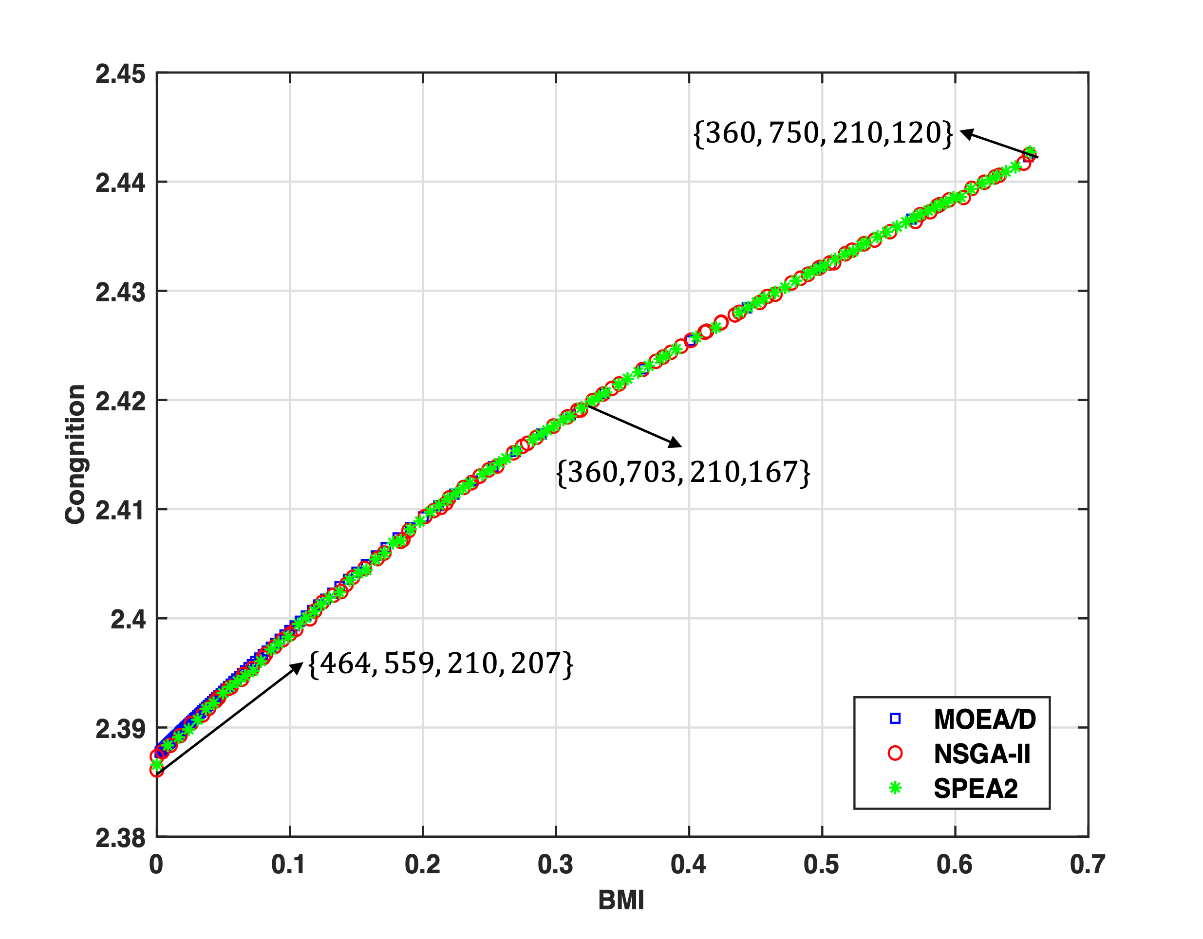
(a) Median HV Run of optimizing BMI and Cognition

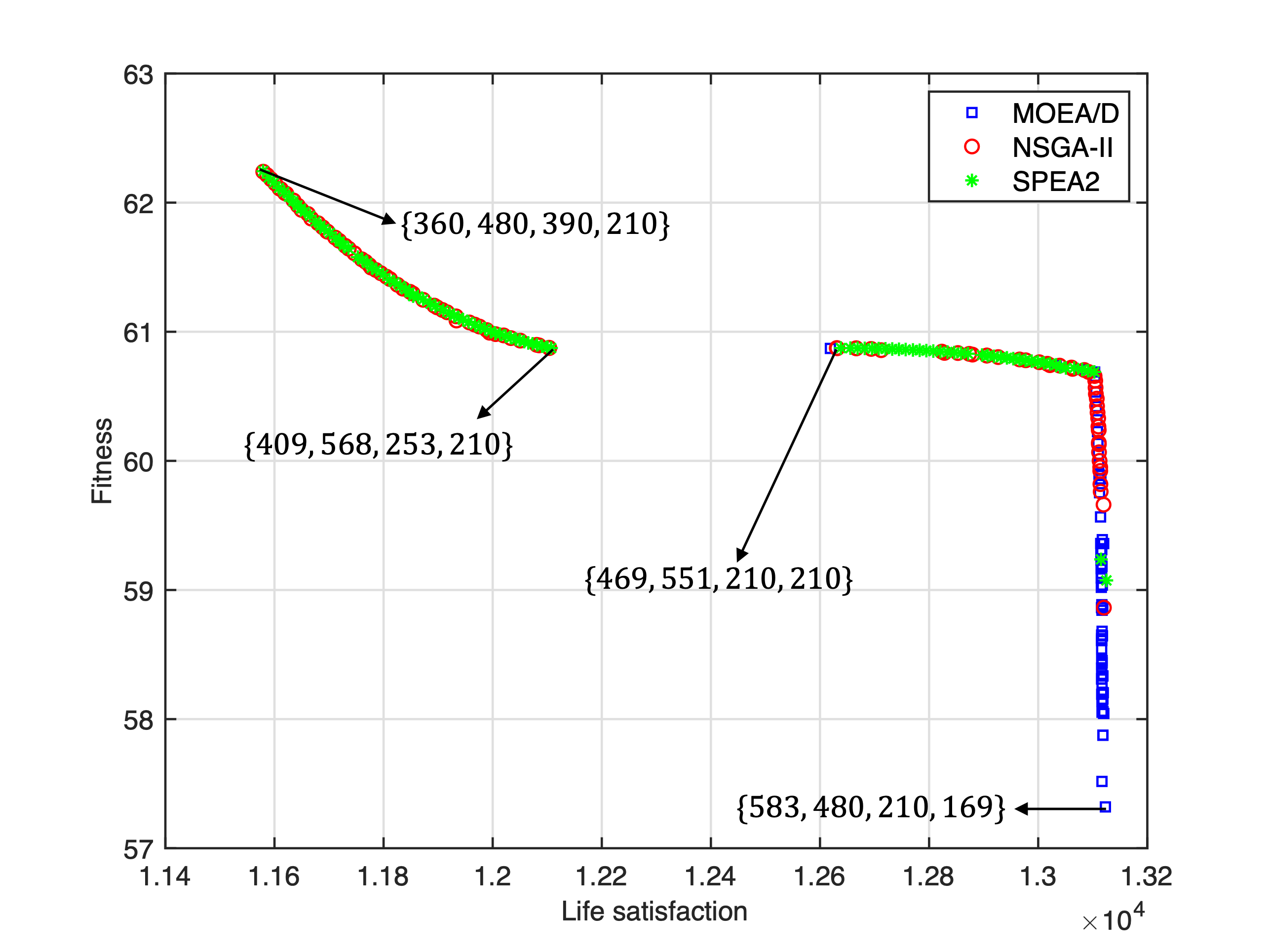
(b) Median HV Run of optimizing Life satisfaction and Fitness

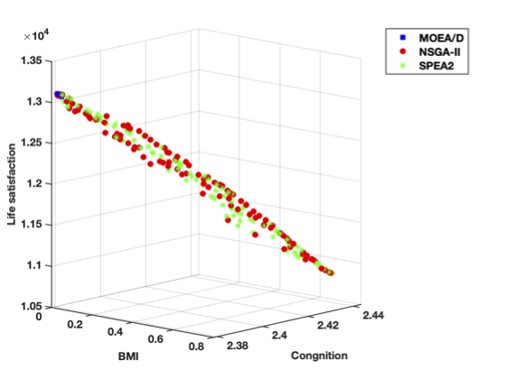
(c) Median HV Run of optimizing BMI, Cognition and Life satisfaction

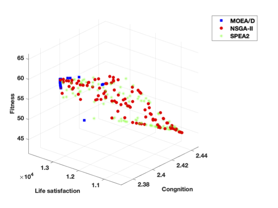
(d) Median HV Run of optimizing Cognition, Life satisfaction and Fitness

Figure 1: Results obtained for multi-objective model of sporty day

Table LABEL:tab:singelresult and Table LABEL:tab:singelweekresult list the results obtained of one-day instances and one-week instances separately. We provide the results from 30 independent runs with $25,000$ generation for all instances. The mean denotes the average objective value of the 30 runs and std denotes standard deviation. Since we aim to minimize the absolute value of BMI, the results listed in the BMI rows are absolute values. The best solutions are bold and shadowed in each row. We also report the decision variables (rounded to minutes) of the optimal solution for each health outcome of each day structure in Table LABEL:tab:singelresult.

Column stat lists the results of statistical comparisons between the algorithms. If two algorithms can be compared significantly, then the index of algorithms that list in each column is significantly worse than the current algorithm. For example, the first row in Table LABEL:tab:singelresult shows that PSO and DE/rand/1 are significantly better than DE/current-to-rand/1 and CMA-ES when optimizing the BMI of Studious day, and DE/current-to-rand/1 is significantly better than CMA-ES. However, there is no significant difference between the performance of DE/rand/1 and PSO. As can be seen from the table of one-day instances, the results obtained by the PSO are better than other algorithms in nearly all cases. DE algorithm with DE/rand/1 operator is the second best algorithm, outperforming the DE algorithm with DE/current-to-rand/1 operator and CMA-ES in many instances, while CMA-ES shows an advantage when aiming to optimize Cognition for many day structures. Moreover, as observed in the std columns, the standard deviation of 30 runs of all the evaluated algorithms in most instances is close to zero. Therefore, we can argue that for the single-objective optimization, the results obtained by the investigated algorithms, especially the DE/rand/1 and PSO, are close to optimal.

Table LABEL:tab:singelweekresult presents the summary statistic for the results of one-week single-objective instances. A closer inspection of the table shows that DE/rand/1 outperforms the other algorithms in most instances, and PSO outperforms the last two algorithms. Therefore, these results suggest that for solving the single-objective optimization problem, DE algorithm with DE/rand/1 operator and PSO both perform well. PSO is preferred for one-day instances, and the DE algorithm with DE/rand/1 operator is preferred for solving one-week instances.

4.2 Results of Multi-objective Time-Use Optimization

To compare the difference between evolutionary multi-objective optimization algorithms, we analyze the experimental results of two, three and four objectives, respectively. For performance evaluation, we use hypervolume [44, 3] as the metric. The hypervolume statistics are provided in Table LABEL:tab:bioresults. The best hypervolume is highlighted and bold for each combination of objectives in each row. It can be seen from the stat results in the table that SPEA significantly outperforms the other algorithms for two-objective optimization instances, and NSGA-II outperforms the other two algorithms for three- and four-objective optimization instances.

The bio-objective results obtained in a median hypervolume run for each algorithm are plotted in Figure 1. Fig. 1 (a) shows that the trade-off fronts of optimizing the first two objectives achieved by SPEA2 are more generally distributed in the Pareto front than MOEA/D and NSGA-II. Similarly, Fig. 1 (b) indicates that the trade-off solutions obtained by MOEA/D and NSGA-II are clustered in a small area of the solution space. Moreover, for three-objective optimization (Fig. 1 (c) and (d)), NSGA-II and SPEA2 generate better Pareto solutions in comparison with MOEA/D. On Fig. 1 (a) and (b), selected optimized solutions are shown to reflect optimal daily activity durations if one individual outcome is preferred above another (near to the respective axes) or if the outcomes are equally preferred (near the mid-point of the Pareto front).

5 Conclusion

The way children spend their time on sleep, sedentary behaviour and physical activity (LPA and MVPA) affects their health and well-being. The main goal of the current study is to implement evolutionary algorithms on daily allocations to optimize children’s health outcomes. Based on a real-world data set, we introduce single- and multi-objective optimization models and design fitness functions of one-day and one-week problems. Our experimental results show that when tackling the single-objective problem, DE algorithm with DE/rand/1 and PSO outperforms other proposed algorithms on both one-day instances and one-week instances. Moreover, the SPEA2 has a higher hypervolume than NSGA-II and MOEA/D in two-objective optimization instances for the multi-objective problem. In comparison, NSGA-II has a higher hypervolume than the other algorithms in three and four objectives instances. Overall, this study strengthens the idea that evolutionary algorithms can be used to enhance our understanding of how children can allocate their daily time to optimize their health and well-being. Parents are concerned about their children’s sleep, screen time and physical activity, and they want evidence-based guidance on how much time should be spent in these behaviours. However, it is unlikely to be feasible to expect families to follow strict daily time allocation schedules. The evidence generated from the application of optimization algorithms may be better understood as general advice, and primarily serve to inform public health guidelines for children’s time-use behaviours. Population-level surveillance of guideline compliance can help inform public health policy, track secular trends overtime and to evaluate the effectiveness of public health interventions.

6 Acknowledgements

This work has been supported by NHMRC Ideas grant 1186123, by ARC grant FT200100536, and by the South Australian Government through the Research Consortium "Unlocking Complex Resources through Lean Processing". Dorothea Dumuid is supported by NHMRC Fellowship 1162166 and by the Centre of Research Excellence in Driving Global Investment in Adolescent Health funded by NHMRC 1171981. The CheckPoint study was supported by the NHMRC [1041352; 1109355]; the National Heart Foundation of Australia [100660]; The Royal Children’s Hospital Foundation [2014-241]; the Murdoch Children’s Research Institute (MCRI); The University of Melbourne; the Financial Markets Foundation for Children [2014-055, 2016-310]; and the Australian Department of Social Services (DSS). Research at the MCRI is supported by the Victorian Government’s Operational Infrastructure Support Program. The funders played no role in the study design, data collection and analysis, decision to publish, or preparation of the manuscript.

References

- [1] J. Aitchison. The statistical analysis of compositional data. Journal of the Royal Statistical Society: Series B (Methodological), 44(2):139–160, 1982.
- [2] M. R. AlRashidi and M. E. El-Hawary. A survey of particle swarm optimization applications in electric power systems. IEEE Trans. Evol. Comput., 13(4):913–918, 2009.
- [3] A. Auger, J. Bader, D. Brockhoff, and E. Zitzler. Hypervolume-based multiobjective optimization: Theoretical foundations and practical implications. Theor. Comput. Sci., 425:75–103, 2012.
- [4] A. Banks, J. Vincent, and C. Anyakoha. A review of particle swarm optimization. part i: background and development. Natural Computing, 6(4):467–484, 2007.
- [5] A. Banks, J. Vincent, and C. Anyakoha. A review of particle swarm optimization. part ii: hybridisation, combinatorial, multicriteria and constrained optimization, and indicative applications. Natural Computing, 7(1):109–124, 2008.
- [6] C. Boreham, V. Paliczka, and A. Nichols. A comparison of the pwc170 and 20-mst tests of aerobic fitness in adolescent schoolchildren. The Journal of sports medicine and physical fitness, 30(1):19–23, 1990.
- [7] G. E. P. Box and D. R. Cox. An analysis of transformations. Journal of the Royal Statistical Society. Series B (Methodological), 26(2):211–252, 1964.
- [8] V. Carson, S. Hunter, N. Kuzik, C. E. Gray, V. J. Poitras, J.-P. Chaput, T. J. Saunders, P. T. Katzmarzyk, A. D. Okely, S. Connor Gorber, et al. Systematic review of sedentary behaviour and health indicators in school-aged children and youth: an update. Applied physiology, nutrition, and metabolism, 41(6):S240–S265, 2016.
- [9] J.-P. Chaput, C. E. Gray, V. J. Poitras, V. Carson, R. Gruber, T. Olds, S. K. Weiss, S. Connor Gorber, M. E. Kho, M. Sampson, et al. Systematic review of the relationships between sleep duration and health indicators in school-aged children and youth. Applied physiology, nutrition, and metabolism, 41(6):S266–S282, 2016.
- [10] S. A. Clifford, S. Davies, and M. Wake. Child health checkpoint: cohort summary and methodology of a physical health and biospecimen module for the longitudinal study of australian children. BMJ open, 9(Suppl 3), 2019.
- [11] C. A. C. Coello, D. A. van Veldhuizen, and G. B. Lamont. Evolutionary algorithms for solving multi-objective problems, volume 5 of Genetic algorithms and evolutionary computation. Kluwer, 2002.
- [12] G. W. Corder and D. I. Foreman. Nonparametric statistics: A step-by-step approach. John Wiley & Sons, 2014.
- [13] S. Das and P. N. Suganthan. Differential evolution: A survey of the state-of-the-art. IEEE transactions on evolutionary computation, 15(1):4–31, 2010.
- [14] K. Deb. Multi-objective optimization using evolutionary algorithms. Wiley-Interscience series in systems and optimization. Wiley, 2001.
- [15] K. Deb, A. Pratap, S. Agarwal, and T. Meyarivan. A fast and elitist multiobjective genetic algorithm: Nsga-ii. IEEE transactions on evolutionary computation, 6(2):182–197, 2002.
- [16] D. Dumuid, T. Olds, K. Lange, B. Edwards, K. Lycett, D. P. Burgner, P. Simm, T. Dwyer, H. Le, and M. Wake. Goldilocks days: optimising children’s time use for health and well-being. J Epidemiol Community Health, 2021.
- [17] D. Dumuid, T. E. Stanford, J.-A. Martin-Fernández, Ž. Pedišić, C. A. Maher, L. K. Lewis, K. Hron, P. T. Katzmarzyk, J.-P. Chaput, M. Fogelholm, et al. Compositional data analysis for physical activity, sedentary time and sleep research. Statistical methods in medical research, 27(12):3726–3738, 2018.
- [18] D. Dumuid, M. Wake, D. Burgner, M. S. Tremblay, A. D. Okely, B. Edwards, T. Dwyer, and T. Olds. Balancing time use for children’s fitness and adiposity: evidence to inform 24-hour guidelines for sleep, sedentary time and physical activity. PloS one, 16(1):e0245501, 2021.
- [19] M. Gray and D. Smart. Growing up in australia: the longitudinal study of australian children is now walking and talking. Family Matters, (79):5–13, 2008.
- [20] L. Han and H. Wang. A random forest assisted evolutionary algorithm using competitive neighborhood search for expensive constrained combinatorial optimization. Memetic Comput., 13(1):19–30, 2021.
- [21] N. Hansen. The CMA evolution strategy: A comparing review. In Towards a New Evolutionary Computation, volume 192 of Studies in Fuzziness and Soft Computing, pages 75–102. Springer, 2006.
- [22] N. Hansen and A. Ostermeier. Completely derandomized self-adaptation in evolution strategies. Evol. Comput., 9(2):159–195, 2001.
- [23] E. H. Houssein, A. G. Gad, K. Hussain, and P. N. Suganthan. Major advances in particle swarm optimization: Theory, analysis, and application. Swarm Evol. Comput., 63:100868, 2021.
- [24] W. Jakob. Applying evolutionary algorithms successfully: A guide gained from real-world applications. CoRR, abs/2107.11300, 2021.
- [25] J. Kennedy and R. Eberhart. Particle swarm optimization. In Proceedings of ICNN’95-international conference on neural networks, volume 4, pages 1942–1948. IEEE, 1995.
- [26] J. Kennedy and R. Eberhart. Particle swarm optimization. In Proceedings of ICNN’95-international conference on neural networks, volume 4, pages 1942–1948. IEEE, 1995.
- [27] K. Lee and J. Kim. Multiobjective particle swarm optimization with preference-based sort and its application to path following footstep optimization for humanoid robots. IEEE Trans. Evol. Comput., 17(6):755–766, 2013.
- [28] X. Li, M. R. Bonyadi, Z. Michalewicz, and L. Barone. Solving a real-world wheat blending problem using a hybrid evolutionary algorithm. In IEEE Congress on Evolutionary Computation, pages 2665–2671. IEEE, 2013.
- [29] G. Mateu-Figueras. The principle of working on coordinates in: Pawlowsky-glahn v, buccianti a, editors. compositional data analysis: theory and applications, 2011.
- [30] A. J. Nebro, J. J. Durillo, and M. Vergne. Redesigning the jmetal multi-objective optimization framework. In GECCO (Companion), pages 1093–1100. ACM, 2015.
- [31] A. D. Okely, D. Ghersi, S. P. Loughran, D. P. Cliff, T. Shilton, R. A. Jones, R. M. Stanley, J. Sherring, N. Toms, S. Eckermann, et al. A collaborative approach to adopting/adapting guidelines. the australian 24-hour movement guidelines for children (5-12 years) and young people (13-17 years): An integration of physical activity, sedentary behaviour, and sleep. International Journal of Behavioral Nutrition and Physical Activity, 19(1):1–21, 2022.
- [32] M. d. Onis, A. W. Onyango, E. Borghi, A. Siyam, C. Nishida, and J. Siekmann. Development of a who growth reference for school-aged children and adolescents. Bulletin of the World health Organization, 85:660–667, 2007.
- [33] R Core Team. R: A Language and Environment for Statistical Computing. R Foundation for Statistical Computing, Vienna, Austria, 2020.
- [34] K. Ridley, T. S. Olds, and A. Hill. The multimedia activity recall for children and adolescents (marca): development and evaluation. International Journal of Behavioral Nutrition and Physical Activity, 3(1):1–11, 2006.
- [35] C. Saha and M. P. Jones. Asymptotic bias in the linear mixed effects model under non-ignorable missing data mechanisms. Journal of the Royal Statistical Society: Series B (Statistical Methodology), 67(1):167–182, 2005.
- [36] J. L. Seligson, E. S. Huebner, and R. F. Valois. Preliminary validation of the brief multidimensional students’ life satisfaction scale (bmslss). Social Indicators Research, 61(2):121–145, 2003.
- [37] R. Storn and K. Price. Differential evolution–a simple and efficient heuristic for global optimization over continuous spaces. Journal of global optimization, 11(4):341–359, 1997.
- [38] K. G. Van den Boogaart and R. Tolosana-Delgado. Analyzing compositional data with R, volume 122. Springer, 2013.
- [39] D. Wang, D. Tan, and L. Liu. Particle swarm optimization algorithm: an overview. Soft Computing, 22(2):387–408, 2018.
- [40] S. Weintraub, S. S. Dikmen, R. K. Heaton, D. S. Tulsky, P. D. Zelazo, P. J. Bauer, N. E. Carlozzi, J. Slotkin, D. Blitz, K. Wallner-Allen, et al. Cognition assessment using the nih toolbox. Neurology, 80(11 Supplement 3):S54–S64, 2013.
- [41] Q. Zhang and H. Li. MOEA/D: A multiobjective evolutionary algorithm based on decomposition. IEEE Trans. Evol. Comput., 11(6):712–731, 2007.
- [42] Y. Zhang, S. Wang, and G. Ji. A comprehensive survey on particle swarm optimization algorithm and its applications. Mathematical problems in engineering, 2015, 2015.
- [43] E. Zitzler, M. Laumanns, and L. Thiele. Spea2: Improving the strength pareto evolutionary algorithm. TIK-report, 103, 2001.
- [44] E. Zitzler and L. Thiele. Multiobjective evolutionary algorithms: a comparative case study and the strength pareto approach. IEEE Trans. Evol. Comput., 3(4):257–271, 1999.