Bayesian nonparametric scalar-on-image regression via Potts-Gibbs random partition models

Abstract

Scalar-on-image regression aims to investigate changes in a scalar response of interest based on high-dimensional imaging data. We propose a novel Bayesian nonparametric scalar-on-image regression model that utilises the spatial coordinates of the voxels to group voxels with similar effects on the response to have a common coefficient. We employ the Potts-Gibbs random partition model as the prior for the random partition in which the partition process is spatially dependent, thereby encouraging groups representing spatially contiguous regions. In addition, Bayesian shrinkage priors are utilised to identify the covariates and regions that are most relevant for the prediction. The proposed model is illustrated using the simulated data sets.

Keywords Bayesian nonparametric  $\cdot$ Gibbs-type priors  $\cdot$ Potts model  $\cdot$ Clustering  $\cdot$ Generalised Swendsen-Wang  $\cdot$ High-dimensional imaging data

1 Introduction

Through advances in data acquisition, vast amounts of high-dimensional imaging data are collected to study phenomena in many fields. Such data are common in biomedical studies to understand a disease or condition of interest Craddock et al. (2009); Fan et al. (2008); Shi et al. (2014); Van Walderveen et al. (1998), and in other fields such as psychology Davatzikos et al. (2005); Sun et al. (2009), social sciences Ferwerda et al. (2016); Hum et al. (2011); Kim and Kim (2018); Samany (2019), economics Henderson et al. (2009); Naik et al. (2016, 2017), climate sciences O’Neill (2013); O’Neill et al. (2013), environmental sciences Debois et al. (2013); Gundlach-Graham et al. (2015); Maloof et al. (2020) and more. While extracting features from the images based on predefined regions of interest favours interpretation and eases computational and statistical issues, changes may occur in only part of a region or span multiple structures. In order to capture the complex spatial pattern of changes and improve accuracy and understanding of the underlying phenomenon, sophisticated approaches are required that utilize the entire high-dimensional imaging data. However, the massive dimension of the images, which is often in the millions, combined with the relatively small sample size, which at best is usually in the hundreds, pose serious challenges.

In the statistical literature, this is framed as a scalar-on-image regression (SIR) problem Goldsmith et al. (2014); Huang et al. (2013); Kang et al. (2018); Li et al. (2015). SIR belongs to the “large p, small n" paradigm; thus, many SIR models utilise shrinkage methods that additionally incorporate the spatial information in the image Goldsmith et al. (2014); Huang et al. (2013); Kang et al. (2018); Lee and Cao (2021); Li et al. (2015); Mehrotra and Maity (2021); Reiss et al. (2011); Smith and Fahrmeir (2007); Wang et al. (2017). In the SIR problem, the covariates represent the image value at a single pixel/voxel, i.e. a very tiny region, and the effect on the response is most often weak, unreliable and difficult to interpret. Moreover, neighbouring pixels/voxels are highly correlated, making standard regression methods, even with shrinkage, problematic due to multicollinearity.

To overcome these difficulties, we develop a novel Bayesian nonparametric (BNP) SIR model that extracts interpretable and reliable features from the images by grouping voxels with similar effects on the response to have a common coefficient. Specifically, we employ the Potts-Gibbs model Lü et al. (2020) as the prior of the random image partition to encourage spatially dependent clustering. In this case, features represent regions that are automatically defined to be the most discriminative. This not only improves the signal and eases interpretability, but also reduces the computational burden by drastically decreasing the image dimension and addressing the multicollinearity problem. Moreover, it allows sharp discontinuities in the coefficient image across regions, which may be relevant in medical applications to capture irregularities Wang et al. (2017).

In this direction, Li et al. (2015) proposed the Ising-DP SIR model, which combines an Ising prior to incorporate the spatial information in the sparsity structure with a Dirichlet Process (DP) prior to group coefficients. Still, the spatial information is only incorporated in the sparsity structure and not in the BNP clustering model, which could result in regions that are dispersed throughout the image. Instead, we propose to incorporate the spatial information in the random partition model, encouraging spatially contiguous regions. Further advantages of the nonparametric model include a data-driven number of clusters, interpretable parameters, and efficient computations. Moreover, we combine this with heavy-tailed shrinkage priors Song and Liang (2017) to identify relevant covariates and regions.

The remainder of this article is organized as follows. Section 2 outlines the development of the SIR model based on the Potts-Gibbs models. Section 3 derives the MCMC algorithm for posterior inference using the generalized Swendsen-Wang (GSW) Xu et al. (2016) algorithm for efficient split-merge moves that take advantage of the spatial structure. Section 4 illustrates the methods through simulation studies. Section 5 concludes with a summary and future work.

2 Model Specification

We introduce the statistical models that form the basis of the proposed Potts-Gibbs SIR model: SIR, random image partition model and shrinkage prior.

2.1 Scalar-on-Image Regression

SIR is a statistical linear method used to study and analyse the relationship between a scalar outcome and two or three-dimensional predictor images under a single regression model Goldsmith et al. (2014); Huang et al. (2013); Kang et al. (2018); Li et al. (2015). For each data point, $i=1,\ldots,n$, we have

$$y_{i}=\text{$\textbf{w}_{i}^{T}$}\boldsymbol{\mu}+\text{$\textbf{x}_{i}^{T}$}\boldsymbol{\beta}+\epsilon_{i},\quad\text{$\epsilon_{i}\stackrel{{\scriptstyle iid}}{{\sim}}\text{N}\left(0,\sigma^{2}\right),$}$$ (1)

where $y_{i}$ is a scalar continuous outcome measure, $\textbf{w}_{i}=(w_{i1},\ldots,w_{iq})^{T}\in\mathbb{R}^{q}$ is a $q$-dimensional vector of covariates, and $\textbf{x}_{i}=(x_{i1},\ldots,x_{ip})^{T}\in\mathbb{R}^{p}$ is a $p$-dimensional image predictor. Each $x_{ij}$ indicates the value of the image at a single pixel with spatial location $\textbf{s}_{j}=(s_{j1},s_{j2})^{T}\in\mathbb{R}^{2}$ for $j=1,\ldots,p$. We define $\boldsymbol{\mu}=(\mu_{1},\ldots,\mu_{q})^{T}\in\mathbb{R}^{q}$ as a $q$-dimensional fixed effects vector and $\boldsymbol{\beta}=\left(\beta(\textbf{s}_{1}),\ldots,\beta(\textbf{s}_{p})\right)^{T}$ (with $\beta_{j}:=\beta(\textbf{s}_{j})$) as the spatially varying coefficient image described on the same lattice as $\textbf{x}_{i}$. We model the high-dimensional $\boldsymbol{\beta}$ by spatially clustering the pixels into $M$ regions and assuming common coefficients $\beta^{*}_{1},\ldots,\beta^{*}_{M}$ within in each cluster, i.e. $\beta_{j}=\beta_{m}^{*}$ given the cluster label $z_{j}=m$. Thus, the prior on the coefficient image is decomposed into two parts: the random image partition model for spatially clustering the pixels and a shrinkage prior for the cluster-specific coefficients $\boldsymbol{\beta}^{*}=\left(\beta^{*}_{1},\ldots,\beta^{*}_{M}\right)^{T}$. The SIR model in (1) can be extended for other types of responses through a generalized linear model framework (GLM) McCullagh and Nelder (2019).

2.2 Random Image Partition Model

The image predictors are observed on a spatially structured coordinate system. Exchangeability is indeed no longer the proper assumption as the images contain covariate information, that we wish to leverage to improve model performance in this high-dimensional setting. To do so, we combine BNP random partition models, which avoid the need to prespecify the number of clusters, allowing it be determined and grow with the data, with a Potts-like spatial smoothness component Potts and Domb (1952). Spatial random partition models in this direction are a growing research area, including Markov random field (MRF) with the product partition model (PPM) Pan et al. (2020), with DP Orbanz and Buhmann (2007); Xu et al. (2016), with Pitman–Yor process (PY)Lü et al. (2020) and with mixture of finite mixtures (MFM) Hu et al. (2020); Zhao et al. (2020). Precisely, within the BNP framework, we focus on the class of Gibbs-type random partitions Cerquetti (2008); Gnedin and Pitman (2006); Lijoi and Prünster (2010); Pitman (2006), motivated by their comprise between tractable predictive rules and richness of the predictive structure, including important cases, such as the DP Ferguson (1973), PY Perman et al. (1992); Pitman (1996), and MFM Miller and Harrison (2018). The Potts-Gibbs models induce a distribution on the partition $\pi_{p}=\{C_{1},\ldots,C_{M}\}$ of $p$ pixels into $M$ nonempty, mutually exclusive, and exhaustive subsets $C_{1},\ldots,C_{M}$ such that $\cup_{C\in\pi_{p}}C=\{1,\ldots,p\}$. The model can be summarised as:

$$\text{pr}(\pi_{p})\propto\exp\underbrace{\left(\sum_{j\sim k,j<k}\upsilon_{jk}\mathbbm{1}_{z_{j}=z_{k}}\right)}_{\text{Potts model}}\underbrace{\left(V_{p}(M)\prod^{M}_{m=1}W_{m}(\phi)\right)}_{\text{Gibbs-type random partition models}},$$

where $z_{j}\in\{1,\cdots,M\}$, $j\sim k$ means that $j$ and $k$ are neighbors, and $\mathbbm{1}_{z_{j}=z_{k}}$ equals to 1 if $j$ and $k$ in the same cluster and 0 otherwise. In the following, we assume the spatial locations lie on a rectangular lattice with first-order neighbors and a common coupling parameter $\upsilon$ for all neighbor pairs; a higher value of $\upsilon$ encourages more spatial smoothness in the partition. We use the general notation $\phi$ to denote the parameters of the Gibbs-type partition models, and focus our study on three cases 1) DP with concentration parameter $\alpha>0$; 2) PY with discount parameter $\delta\in[0,1)$ and concentration parameter $\alpha>-\delta$; and 3) MFM with parameter $\gamma>0$ (larger values encouraging more equally sized clusters) and a distribution $P_{L}(\cdot|\lambda)$ with parameter $\lambda$ related to the prior on the number of clusters. The $\{V_{p}(M):p\geq 1,1\leq M\leq p\}$ denotes the set of non-negative weights, which solves the backward recurrence relation $V_{p}(M)=(p-\delta M)V_{p+1}(M)+V_{p+1}(M+1)$ with $V_{1}(1)=1$. Table 1 describes the $V_{p}(M)$ and $W_{m}(\phi)$ for DP, PY and MFM models.

Table 1: Formulas of $V_{p}(M),W_{m}(\phi)$ and terms of the predictive probability for assigning current cluster to either existing cluster or new cluster for DP, PY and MFM. Note that the predictive probabilities are stated up to a proportionality constant.

	DP	PY	MFM
$V_{p}(M)$	$\frac{\Gamma(\alpha)\alpha^{M}}{\Gamma(\alpha+p)}$	$\frac{\Gamma(\alpha+1)\prod_{m=1}^{M-1}(\alpha+m\delta)}{\Gamma(\alpha+p)}$	$\sum_{l=1}^{\infty}\frac{\Gamma(\gamma l)l!}{\Gamma(\gamma l+p)(l-m)!}P_{L}(\cdot|\lambda)$
$W_{m}(\phi)$	$\Gamma(\mid C_{m}\mid)$	$\frac{\Gamma(\mid C_{m}\mid-\delta)}{\Gamma(1-\delta)}$	$\frac{\Gamma(\mid C_{m}\mid+\gamma)}{\Gamma(\gamma)}$
Existing cluster	$\frac{\Gamma(|C_{m}^{-A_{o}}|+|A_{o}|)}{\Gamma(|C_{m}^{-A_{o}}|)}$	$\frac{\Gamma(|C_{m}^{-A_{o}}|+|A_{o}|-\delta)}{\Gamma(|C_{m}^{-A_{o}}|-\delta)}$	$\frac{\Gamma(|C_{m}^{-A_{o}}|+|A_{o}|+\gamma)}{\Gamma(|C_{m}^{-A_{o}}|+\gamma)}$
New cluster	$\alpha\Gamma(|A_{o}|)$	$(\alpha+\delta M^{-A_{o}})\frac{\Gamma(|A_{o}|-\delta)}{\Gamma(1-\delta)}$	$\frac{V_{p}(M^{-A_{o}}+1)}{V_{p}(M^{-A_{o}})}\frac{\Gamma(|A_{o}|+\gamma)}{\Gamma(\gamma)}$

2.3 Shrinkage Prior

To identify relevant regions, we use heavy tailed priors for the unique values $(\beta_{1}^{*},\ldots,\beta_{M}^{*})$ of $\left(\beta(\textbf{s}_{1}),\ldots,\beta(\textbf{s}_{p})\right)$. Specifically, a $t$-shrinkage prior is used, motivated by its computational efficiency and nearly optimal contraction rate and selection consistency Song and Liang (2017):

$$\sigma^{2} \sim\text{IG}\left(a_{\sigma},b_{\sigma}\right),$$ (2)

$$\left(\beta_{m}^{*}\right)|\sigma^{2} \sim t_{\nu}(s\sigma),\quad\text{for all }m=1,\ldots,M,$$

where $t_{\nu}(s\sigma)$ denotes $t$-distribution with degree of freedom $\nu$ and scale parameter $s\sigma$. For posterior inference, the $t$-distribution (2) is rewritten as a hierarchical inverse-gamma scaled Gaussian mixture,

$$\sigma^{2} \sim\text{IG}\left(a_{\sigma},b_{\sigma}\right),$$

$$\eta_{m}^{*} \sim\text{IG}\left(a_{\eta},b_{\eta}\right),$$

$$\left(\beta_{m}^{*}\right)|\sigma^{2},\eta_{m}^{*} \sim N(0,\eta_{m}^{*}\sigma^{2}),\quad\text{for all }m=1,\ldots,M,$$

where $a_{\eta}$ and $b_{\eta}$ are the shape and scaling parameter of the mixing distribution for each $\eta_{m}^{*}$ respectively with $\nu=2a_{\eta}$ and $s=\sqrt{b_{\eta}/a_{\eta}}$.

3 Inference

We aim to infer the posterior distribution of the parameters based on the proposed Potts-Gibbs SIR model:

$$y_{i}\mid\boldsymbol{\mu},\boldsymbol{\beta}^{*},\pi_{p},\sigma^{2} \sim\text{N}(\textbf{w}_{i}^{T}\boldsymbol{\mu}+\textbf{x}_{i}^{*T}\boldsymbol{\beta}^{*},\sigma^{2}),\quad\text{for all $i=1,\ldots,n$},$$

$$\boldsymbol{\mu}\mid\sigma^{2} \sim\text{N}(\textbf{m}_{\mu},\sigma^{2}\Sigma_{\mu}),$$

$$\boldsymbol{\beta}^{*}\mid\boldsymbol{\eta}^{*},\sigma^{2} \sim\text{N}(\mathbf{0}_{M},\sigma^{2}\Sigma_{\beta^{*}}),$$

$$\sigma^{2} \sim\text{IG}(a_{\sigma},b_{\sigma}),$$

$$\eta_{m}^{*} \sim\text{IG}\left(a_{\eta},b_{\eta}\right),\quad\text{for all $m=1,\ldots,M$},$$

$$\pi_{p} \sim\text{Potts-Gibbs}(\upsilon,\phi),$$

where $x_{im}^{*}=\sum^{p}_{j=1}x_{ij}\mathbbm{1}(j\in C_{m})/\sqrt{\mid C_{m}\mid}$ represents the total value, e.g. volume in the $m$th region of the image, $\textbf{m}_{\mu}=(m_{\mu_{1}},\ldots,m_{\mu_{q}})$, $\Sigma_{\mu}=\text{diag}(c_{\mu_{1}},\ldots,c_{\mu_{q}})^{T}$, and $\Sigma_{\beta^{*}}=\text{diag}(\eta_{1}^{*},\ldots,\eta^{*}_{{}_{M}})$. Note that when defining $x_{im}^{*}$, we rescale by the square root of cluster size , which is equivalent to rescaling the variance of $\beta^{*}_{m}$ by the cluster size, encouraging more shrinkage for larger regions.

We develop a Gibbs sampler to simulate from the posterior with a generalized Swendsen-Wang (GSW) algorithm to draw samples from the Potts-Gibbs model. Poor mixing can be seen in single-site Gibbs sampling Geman and Geman (1984) due to the high correlation between the pixel labels. The SW algorithm Swendsen and Wang (1987) addresses this by forming nested clusters of neighbouring pixels, then updating all of the labels within a nested cluster to the same value. The generalisation of the technique for standard Potts models to generalised Potts-partition models is called GSW Xu et al. (2016). At each step of the algorithm, we proceed through the following steps:

1. Sample the image partition $\pi_{p}$ given $\boldsymbol{\eta}^{*}$ and the data (with $\boldsymbol{\beta}^{*},\boldsymbol{\mu},\sigma^{2}$ marginalized). GSW is used to update simultaneously nested groups of pixels and hence improve the exploration of the posterior. The algorithm relies on the introduction of auxiliary binary bond variables, where $r_{jk}=1$ if pixels $j$ and $k$ are bonded, otherwise 0. The bond variables define a partition of the pixels into nested clusters $A_{1},\ldots,A_{O}$, where $O$ denotes the number of nested clusters and each $A_{o}\subseteq C_{m}$ for some $m=1,\ldots,M$. For each neighbor pair $j\sim k$ for $1\leq j<k\leq p$, we sample the bond variables as follows, $r_{jk}\sim\text{Ber}\{1-\exp(-\upsilon_{jk}\zeta_{jk}\mathbbm{1}_{z_{j}=z_{k}})\}$, where we define $\zeta_{jk}=\kappa\exp\{-\tau d(\hat{\beta}_{j},\hat{\beta}_{k})\}$ with $\hat{\beta}_{j}$ denoting the estimated coefficient from univariate regression on the $j$th pixel and $\kappa,\tau$ are the tuning parameters of the GSW sampler. Notice that the algorithm reduces to single-site Gibbs when $\kappa=0$, and recovers classical SW when $\kappa=1$ and $\tau=0$.

   As we are dealing with non-conjugate priors, we update the cluster assignment by extending Gibbs sampling with the addition of auxiliary parameters, which is widely known as Algorithm 8 Neal (2000). We denote by $A_{o}$ the current nested cluster; $C_{1}^{-A_{o}},\ldots,C_{M}^{-A_{o}}$ the clusters without nested cluster $A_{o}$; $M^{-A_{o}}$ the number of distinct clusters excluding $A_{o}$ and $h$ the number of temporary auxiliary variables. For each nested cluster $A_{o}$, it is assigned to an existing cluster $m=1,\ldots,M^{-A_{o}}$ or a new cluster $m=M^{-A_{o}}+1,\ldots,M^{-A_{o}}+h$ with probability as follows,

   $$\text{pr}(A_{o}\in C_{m}^{-A_{o}}\mid\cdots)$$

   $$\propto\begin{cases}\frac{\Gamma(|C_{m}^{-A_{o}}|+|A_{o}|-\delta)}{\Gamma(|C_{m}^{-A_{o}}|-\delta)}\text{pr}\left(\textbf{y}\mid\pi_{p}^{A_{o}\rightarrow m},\boldsymbol{\eta^{*}}\right)\\ \prod_{\{(j,k)\mid j\in A_{o},k\in C_{m}^{-A_{o}},r_{jk}=0\}}\exp\left\{\upsilon_{jk}(1-\zeta_{jk})\right\},&\text{for }C_{m}^{-A_{o}}\in\pi_{p}^{-A_{o}},\\ \\ \frac{1}{h}\frac{V_{p}(M^{-A_{o}}+1)}{V_{p}(M^{-A_{o}})}\frac{\Gamma(|A_{o}|-\delta)}{\Gamma(1-\delta)}\text{pr}\left(\textbf{y}\mid\pi_{p}^{A_{o}\rightarrow M+1},\boldsymbol{\eta^{*}}\right),&\text{for new $C_{m}^{-A_{o}}$};\end{cases}$$

   where $\text{pr}\left(\textbf{y}\mid\pi_{p}^{A_{o}\rightarrow m},\boldsymbol{\eta^{*}}\right)$ and $\text{pr}\left(\textbf{y}\mid\pi_{p}^{A_{o}\rightarrow M+1},\boldsymbol{\eta^{*}}\right)$ denote the marginal likelihood of data obtained by moving $A_{o}$ from its current cluster to existing clusters or newly created cluster respectively. Before updating the cluster assignments, we sample the nested clusters and compute the volume of each nested cluster for all images, with computational cost $\mathcal{O}(np)$. When updating the cluster assignments, the marginal likelihood dominates the computational cost, as it involves inversion and determinants of $(M+q)\times(M+q)$ matrices and updating the sufficient statistics for every nested cluster and every outer cluster allocation, i.e. the cost is $\mathcal{O}([[M+q]^{3}+n[M+q]]OM)$.

2. Sample $\boldsymbol{\beta}^{*},\boldsymbol{\mu},\sigma^{2}$ jointly given the partition $\pi_{p}$, $\boldsymbol{\eta}^{*}$ and the data. Notationally, we reformulate $\tilde{\textbf{x}}_{i}=(\textbf{w}_{i}^{T},\textbf{x}^{*\,T}_{i})^{T}$ and $\tilde{\boldsymbol{\beta}}=(\boldsymbol{\mu}^{T},\boldsymbol{\beta}^{*\,T})^{T}$. We define $\tilde{\textbf{X}}$ be the matrix with rows equal to $\tilde{\textbf{x}}_{i}^{T}$. The corresponding full conditional for $\tilde{\boldsymbol{\beta}}$ and $\sigma^{2}$ is

   $$\sigma^{2}\mid\cdots\sim \text{IG}(\hat{a}_{\sigma},\hat{b}_{\sigma}),$$

   $$\tilde{\boldsymbol{\beta}}\mid\sigma^{2},\cdots\sim \text{N}(\hat{\textbf{m}}_{\tilde{\beta}},\sigma^{2}\hat{\Sigma}_{\tilde{\beta}}),$$

   where $\hat{\Sigma}_{\tilde{\beta}}=(\Sigma_{\tilde{\beta}}^{-1}+\tilde{\textbf{X}}^{T}\tilde{\textbf{X}})^{-1}$, $\hat{\textbf{m}}_{\tilde{\beta}}=\hat{\Sigma}_{\tilde{\beta}}(\Sigma_{\tilde{\beta}}^{-1}\textbf{m}_{\tilde{\beta}}+\tilde{\textbf{X}}^{T}\textbf{y})$, and $\text{IG}(\hat{a}_{\sigma},\hat{b}_{\sigma})$ denotes the inverse-gamma distribution with updated shape $\hat{a}_{\sigma}=a_{\sigma}+n/2$ and scale $\hat{b}_{\sigma}=b_{\sigma}+[\textbf{m}_{\tilde{\beta}}^{T}\Sigma_{\tilde{\beta}}^{-1}\textbf{m}_{\tilde{\beta}}+\textbf{y}^{T}\textbf{y}-\hat{\textbf{m}}_{\tilde{\beta}}^{T}\hat{\Sigma}_{\tilde{\beta}}^{-1}\hat{\textbf{m}}_{\tilde{\beta}}]/2$.

3. Sample $\boldsymbol{\eta}^{*}$ given $\boldsymbol{\beta}^{*}$. The corresponding full conditional for each $\eta_{m}^{*}$ is an inverse-gamma distribution with updated shape $\hat{a}_{\eta}=a_{\eta}+1/2$ and scale $\hat{b}_{\eta}=b_{\eta}+(\beta^{*}_{m})^{2}/(2\sigma^{2})$:

   $$\eta_{m}^{*}\mid\cdots\sim\text{IG}(\hat{a}_{\eta},\hat{b}_{\eta}),\quad\text{for $m=1,\ldots,M$}.$$

4 Numerical Studies

We study through simulations the performance of the proposed model and compare it with Ising-DP Li et al. (2015). We consider 2D images in this simulation. The $n=300$ images are simulated on a two dimensional grid of size $10\times 10$, with spatial locations $\textbf{s}_{j}=(s_{j1},s_{j2})\in\mathbf{R}^{2}$ for $1\leq s_{j1},s_{j2}\leq 10$. For simplicity’s sake, we include an intercept but do not consider others covariates, $\textbf{w}_{i}$. We concentrate on the two simulation scenarios with true $M=2$ and $M=5$ as shown in Figures 1 - 2. For each experiment, we summarise the posterior of the clustering structure of the data sets by minimising the posterior expected Variation of Information (VI) Wade and Ghahramani (2018).

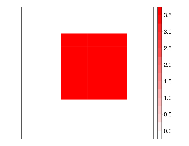
(a) Scenario 1: Truth

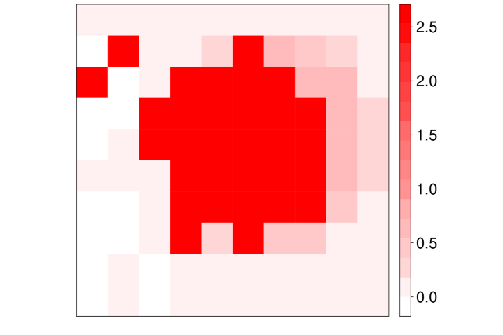
(b) Scenario 1: Ising-DP

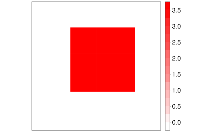
(c) Scenario 1: Potts-DP

(d) Scenario 1: Potts-PY

(e) Scenario 1: Potts-MFM

Figure 1: Figures on the upper and bottom row showing the true and estimated coefficient matrix of the simulated data sets for scenario 1 under each model.

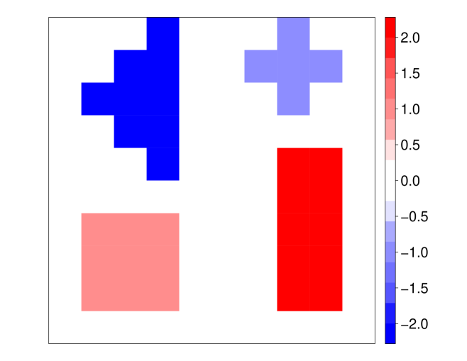
(a) Scenario 2: Truth

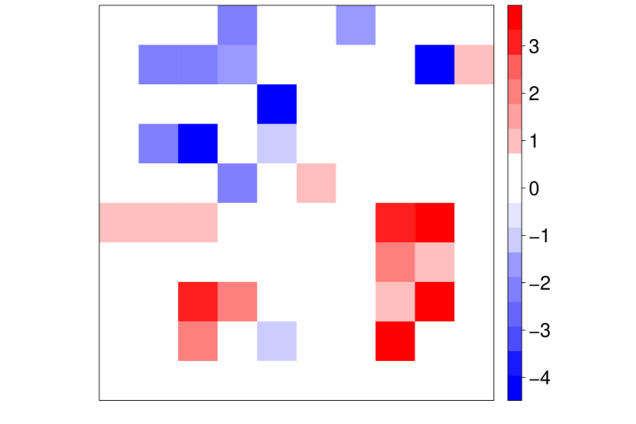
(b) Scenario 2: Ising-DP

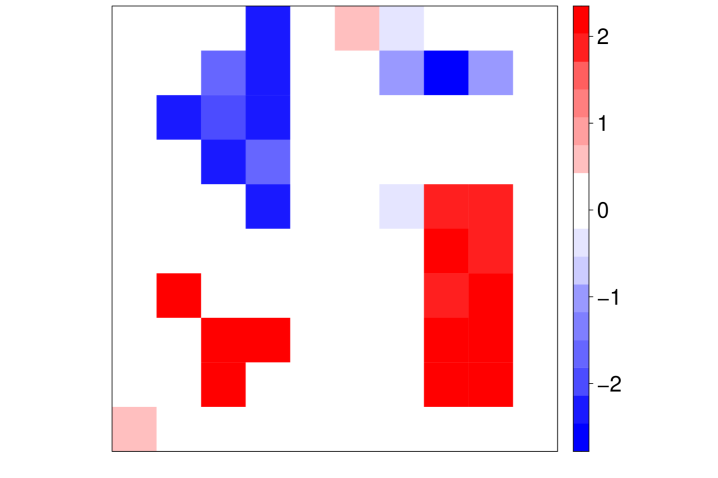
(c) Scenario 2: Potts-DP

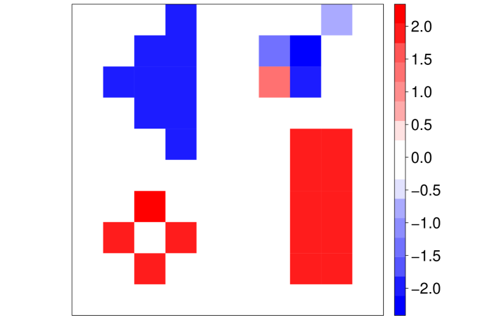
(d) Scenario 2: Potts-PY

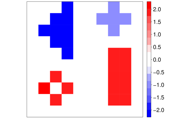
(e) Scenario 2: Potts-MFM

Figure 2: Figures on the upper and bottom row showing the true and estimated coefficient matrix of the simulated data sets for scenario 2 under each model.

The Potts-Gibbs models can detect correctly the cluster structure under scenario 1 (Figure 1). The Potts-Gibbs models are also capable of capturing and identifying the more complex cluster structure underlying the data for scenario 2 (Figure 2) with the ARI 0.621 - 0.830 (Table 2). On the contrary, Ising-DP has failed terribly to recover the cluster structure for scenario 2, as illustrated in Figure 2. It is observed that under the Potts-Gibbs models, most of the resultant clusters are spatially proximal, while under Ising-DP, the clusters are dispersed throughout the image. By taking into consideration spatial dependence in the random partition model via the Potts-Gibbs models, the proposed models produce spatially aware clustering and thus improve the predictions.

DP has a concentration parameter $\alpha$, with larger values encouraging more new clusters and a rich-get-richer property that favours allocation to larger clusters. The PY has an additional discount parameter $\delta\in[0,1)$ that helps to mitigate the rich-get-richer property and phase transition of the Potts model. The MFM has a parameter $\gamma$, with larger values encouraging more equal-sized clusters and helping to avoid phase transition of the Potts model, as well as additional parameters $\lambda$ which are related to the prior on the number of clusters.

Scenario 1
	ARI	VI	MSE	MSPE	$M$
Potts-DP	1.0 (0.004)	0.001 (0.010)	1.33e-4 (5.59e-4)	4.215 (0.057)	2.019 (0.138)
Potts-PY	1.0 (0.004)	0.001 (0.009)	1.03e-4 (8.73e-5)	4.213 (0.052)	2.015 (0.122)
Potts-MFM	0.999 (0.007)	0.001 (0.014)	1.01e-4 (8.37e-5)	4.209 (0.052)	2.007 (0.081)
Ising-DP	0.307 (0.079)	1.386 (0.154)	0.807 (0.011)	145.912 (10.051)	4.575 (1.340)
Scenario 2
	ARI	VI	MSE	MSPE	$M$
Potts-DP	0.621(0.060)	1.160 (0.211)	0.246 (0.064)	7.754 (2.653)	6.722 (0.901)
Potts-PY	0.713 (0.050)	1.006 (0.147)	0.157 (0.035)	0.868 (0.168)	6.882 (1.090)
Potts-MFM	0.830 (0.036)	0.599 (0.133)	0.093 (0.014)	0.850 (0.122)	5.232 (0.475)
Ising-DP	0.038 ( 0.021)	3.990 (0.159)	0.980 ( 0.025)	3.641 (0.526)	15.542 (1.554)

Table 2: Mean and standard deviation of the posterior of adjusted Rand index (ARI), variation information (VI), mean squared error (MSE), mean squared prediction error (MSPE), and number of clusters for each scenario under each model.

5 Conclusion

We have developed novel Bayesian scalar-on-image regression models to extract interpretable features from the image by clustering and leveraging the spatial coordinates of the pixels/voxels. To encourage groups representing spatially contiguous regions, we incorporate the spatial information directly in the prior for the random partition through Potts-Gibbs random partition models. We have shown the potential of Potts-Gibbs models in detecting the correct cluster structure on simulated data sets. In our experiments, the hyperparameters of the Potts-Gibbs model were determined via a simple grid search on selected combinations of hyperparameters. However, future work will consist of investigating the influence of the various parameters inherent to the model and guidelines and tools to determine hyperparameters. The model will then be applied to real images, e.g. neuroimages. Motivated by examining and identifying brain regions of interest in Alzheimer’s disease, we will use MRI images obtained from the Alzheimer’s Disease Neuroimaging Initiative (ADNI) database (www.adni-info.org). The proposed SIR model will be extended to classification problems through the GLM framework.

References

- Craddock et al. [2009] R. Cameron Craddock, Paul E Holtzheimer III, Xiaoping P Hu, and Helen S Mayberg. Disease state prediction from resting state functional connectivity. Magn. Reson. Med., 62(6):1619–1628, 2009. ISSN 0740-3194.
- Fan et al. [2008] Yong Fan, Susan M Resnick, Xiaoying Wu, and Christos Davatzikos. Structural and functional biomarkers of prodromal Alzheimer’s disease: A high-dimensional pattern classification study. NeuroImage, 41(2):277–285, 2008. ISSN 1053-8119.
- Shi et al. [2014] Jie Shi, Natasha Lepore, Boris Gutman, Paul Thompson, Leslie Baxter, Richard Caselli, and Yalin Wang. Genetic influence of apolipoprotein E4 genotype on hippocampal morphometry: An N = 725 surface-based Alzheimer’s disease neuroimaging initiative study. Hum. Brain Mapp., 35(8):3903–3918, 2014. ISSN 1065-9471.
- Van Walderveen et al. [1998] M.A.A Van Walderveen, W Kamphorst, P Scheltens, J.H.T.M Van Waesberghe, R Ravid, J Valk, C.H Polman, and F Barkhof. Histopathologic correlate of hypointense lesions on T1-weighted spin-echo MRI in multiple sclerosis. Neurology, 50(5):1282–1288, 1998. ISSN 0028-3878.
- Davatzikos et al. [2005] Christos Davatzikos, Dinggang Shen, Ruben C Gur, Xiaoying Wu, Dengfeng Liu, Yong Fan, Paul Hughett, Bruce I Turetsky, and Raquel E Gur. Whole-brain morphometric study of schizophrenia revealing a spatially complex set of focal abnormalities. Arch. Gen. Psychiatry, 62(11):1218–1227, 2005. ISSN 0003-990X.
- Sun et al. [2009] Daqiang Sun, Theo G.M van Erp, Paul M Thompson, Carrie E Bearden, Melita Daley, Leila Kushan, Molly E Hardt, Keith H Nuechterlein, Arthur W Toga, and Tyrone D Cannon. Elucidating a magnetic resonance imaging-based neuroanatomic biomarker for psychosis: Classification analysis using probabilistic brain atlas and machine learning algorithms. Biol. Psychiatry (1969), 66(11):1055–1060, 2009. ISSN 0006-3223.
- Ferwerda et al. [2016] Bruce Ferwerda, Markus Schedl, and Marko Tkalcic. Using instagram picture features to predict users’ personality. In International conference on multimedia modeling. Springer, 2016.
- Hum et al. [2011] Noelle J Hum, Perrin E Chamberlin, Brittany L Hambright, Anne C Portwood, Amanda C Schat, and Jennifer L Bevan. A picture is worth a thousand words: A content analysis of Facebook profile photographs. Comput. Hum. Behav., 27(5):1828–1833, 2011. ISSN 0747-5632.
- Kim and Kim [2018] Yunhwan Kim and Jang Hyun Kim. Using computer vision techniques on instagram to link users’ personalities and genders to the features of their photos: An exploratory study. Inf. Process. Manage., 54(6):1101–1114, 2018. ISSN 0306-4573.
- Samany [2019] Najmeh Neysani Samany. Automatic landmark extraction from geo-tagged social media photos using deep neural network. Cities, 93:1–12, 2019. ISSN 0264-2751.
- Henderson et al. [2009] J. Vernon Henderson, Adam Storeygard, and David N Weil. Measuring economic growth from outer space. National Bureau of Economic Research, Cambridge, Mass, 2009.
- Naik et al. [2016] Nikhil Naik, Ramesh Raskar, and César A Hidalgo. Cities are physical too: Using computer vision to measure the quality and impact of urban appearance. Am. Econ. Rev., 106(5):128–132, 2016. ISSN 0002-8282.
- Naik et al. [2017] Nikhil Naik, Scott Duke Kominers, Ramesh Raskar, Edward L Glaeser, and César A Hidalgo. Computer vision uncovers predictors of physical urban change. Proc. Natl. Acad. Sci. U.S.A., 114(29):7571–7576, 2017. ISSN 0027-8424.
- O’Neill [2013] Saffron J O’Neill. Image matters: Climate change imagery in US, UK and Australian newspapers. Geoforum, 49:10–19, 2013. ISSN 0016-7185.
- O’Neill et al. [2013] Saffron J O’Neill, Maxwell Boykoff, Simon Niemeyer, and Sophie A Day. On the use of imagery for climate change engagement. Glob. Environ. Change, 23(2):413–421, 2013. ISSN 0959-3780.
- Debois et al. [2013] Delphine Debois, Marc Ongena, Hélène Cawoy, and Edwin De Pauw. MALDI-FTICR MS imaging as a powerful tool to identify Paenibacillus antibiotics involved in the inhibition of plant pathogens. J. Am. Soc. Mass Spectrom., 24(8):1202–1213, 2013. ISSN 1044-0305.
- Gundlach-Graham et al. [2015] Alexander Gundlach-Graham, Marcel Burger, Steffen Allner, Gunnar Schwarz, Hao A. O Wang, Luzia Gyr, Daniel Grolimund, Bodo Hattendorf, and Detlef Günther. High-speed, high-resolution, multielemental laser ablation-inductively coupled plasma-time-of-flight mass spectrometry imaging: Part i. instrumentation and two-dimensional imaging of geological samples. Anal. Chem., 87(16):8250–8258, 2015. ISSN 0003-2700.
- Maloof et al. [2020] Katherine A Maloof, Alexis N Reinders, and Kevin R Tucker. Applications of mass spectrometry imaging in the environmental sciences. Curr. Opin. Environ. Sci. Health., 18:54–62, 2020. ISSN 2468-5844.
- Goldsmith et al. [2014] Jeff Goldsmith, Lei Huang, and Ciprian M. Crainiceanu. Smooth scalar-on-image regression via spatial Bayesian variable selection. J. Comput. Graph Stat., 23(1):46–64, 2014. ISSN 15372715.
- Huang et al. [2013] Lei Huang, Jeff Goldsmith, Philip T. Reiss, Daniel S. Reich, and Ciprian M. Crainiceanu. Bayesian scalar-on-image regression with application to association between intracranial DTI and cognitive outcomes. NeuroImage, 83:210–223, 2013. ISSN 10538119.
- Kang et al. [2018] Jian Kang, Brian J. Reich, and Ana Maria Staicu. Scalar-on-image regression via the soft-thresholded Gaussian process. Biometrika, 105(1):165–184, 2018. ISSN 14643510.
- Li et al. [2015] Fan Li, Tingting Zhang, Quanli Wang, Marlen Z. Gonzalez, Erin L. Maresh, and James A. Coan. Spatial Bayesian variable selection and grouping for high-dimensional scalar-on-image regression. Ann. Appl. Stat., 9(2):687–713, 2015. ISSN 19417330.
- Lee and Cao [2021] Kyoungjae Lee and Xuan Cao. Bayesian group selection in logistic regression with application to MRI data analysis. Biometrics, 77(2):391–400, 2021. ISSN 0006-341X.
- Mehrotra and Maity [2021] Suchit Mehrotra and Arnab Maity. Simultaneous variable selection, clustering, and smoothing in function-on-scalar regression. Can. J. Stat., 2021. ISSN 0319-5724.
- Reiss et al. [2011] P.T. Reiss, M. Mennes, E. Petkova, L. Huang, M.J. Hoptman, B.B. Biswal, S.J. Colcombe, X. Zuo, and M.P. Milham. Extracting information from functional connectivity maps via function-on-scalar regression. NeuroImage, 56:140–148, 2011.
- Smith and Fahrmeir [2007] Michael Smith and Ludwig Fahrmeir. Spatial Bayesian variable selection with application to functional magnetic resonance imaging. J. Am. Stat. Assoc., 102(478):417–431, 2007. ISSN 0162-1459.
- Wang et al. [2017] Xiao Wang, Hongtu Zhu, and Alzheimer’s Disease Neuroimaging Initiative. Generalized scalar-on-image regression models via total variation. J. Am. Stat. Assoc., 112(519):1156–1168, 2017.
- Lü et al. [2020] Hongliang Lü, Julyan Arbel, and Florence Forbes. Bayesian nonparametric priors for hidden Markov random fields. Stat. Comput., 30(4):1015–1035, 2020. ISSN 0960-3174.
- Song and Liang [2017] Q. Song and F. Liang. Nearly optimal Bayesian shrinkage for high dimensional regression. arXiv:1712.08964, 2017.
- Xu et al. [2016] Richard Yi Da Xu, Francois Caron, and Arnaud Doucet. Bayesian nonparametric image segmentation using a generalized Swendsen-Wang algorithm. arXiv:1602.03048, 2016.
- McCullagh and Nelder [2019] Peter McCullagh and John A Nelder. Generalized linear models. Routledge, 2019.
- Potts and Domb [1952] R. B. Potts and C. Domb. Some generalized order-disorder transformations. Math. Proc. Cambridge Philos. Soc., 48(1):106, January 1952. doi:10.1017/S0305004100027419.
- Pan et al. [2020] Tianyu Pan, Guanyu Hu, and Weining Shen. Identifying latent groups in spatial panel data using a Markov random field constrained product partition model. arXiv:2012.10541, 2020.
- Orbanz and Buhmann [2007] Peter Orbanz and Joachim M Buhmann. Nonparametric Bayesian image segmentation. Int. J. Comput. Vis., 77(1-3):25–45, 2007. ISSN 0920-5691.
- Hu et al. [2020] Guanyu Hu, Junxian Geng, Yishu Xue, and Huiyan Sang. Bayesian spatial homogeneity pursuit of functional data: an application to the U.S. income distribution. arXiv:2002.06663, 2020.
- Zhao et al. [2020] Peng Zhao, Hou-Cheng Yang, Dipak K Dey, and Guanyu Hu. Bayesian spatial homogeneity pursuit regression for count value data. arXiv:2002.06678, 2020.
- Cerquetti [2008] A. Cerquetti. Generalized Chinese restaurant construction of exchangeable Gibbs partitions and related results. arXiv:0805.3853, 2008.
- Gnedin and Pitman [2006] Alexander Gnedin and Jim Pitman. Exchangeable Gibbs partitions and Stirling triangles. J. Math. Sci., 138(3):5674–5685, 2006.
- Lijoi and Prünster [2010] Antonio Lijoi and Igor Prünster. Models beyond the Dirichlet process. In Bayesian Nonparametrics, 2010.
- Pitman [2006] Jim Pitman. Lecture Notes in Mathematics. Springer, 2006. ISBN 1-280-62579-1.
- Ferguson [1973] Thomas S Ferguson. A Bayesian analysis of some nonparametric problems. Ann. Stat., 1:209–230, 1973.
- Perman et al. [1992] Mihael Perman, Jim Pitman, and Marc Yor. Size-biased sampling of Poisson point processes and excursions. Probab. Theory Relat. Fields, 92(1):21–39, 1992.
- Pitman [1996] Jim Pitman. Some developments of the Blackwell-Macqueen urn scheme. Lecture Notes-Monograph Series, 30:245–267, 1996. ISSN 0749-2170.
- Miller and Harrison [2018] Jeffrey W Miller and Matthew T Harrison. Mixture models with a prior on the number of components. J. Am. Stat. Assoc., 113(521):340–356, 2018.
- Geman and Geman [1984] Stuart Geman and Donald Geman. Stochastic relaxation, Gibbs distributions, and the Bayesian restoration of images. IEEE Trans. Pattern Anal. Mach. Intell., (6):721–741, 1984. ISSN 0162-8828.
- Swendsen and Wang [1987] Robert H Swendsen and Jian-Sheng Wang. Nonuniversal critical dynamics in Monte Carlo simulations. Phys. Rev. Lett., 58(2):86–88, 1987. ISSN 0031-9007.
- Neal [2000] Radford M Neal. Markov chain sampling methods for Dirichlet process mixture models. J. Comput. Graph Stat., 9(2):249–265, 2000. ISSN 1061-8600.
- Wade and Ghahramani [2018] Sara Wade and Zoubin Ghahramani. Bayesian cluster analysis: Point estimation and credible balls (with discussion). Bayesian Anal., 13(2):559–626, Jun 2018. ISSN 1936-0975.