Neutrino-nucleus CC0$\pi$ cross-section tuning in GENIE v3

Abstract

This article summarizes the state of the art of $\nu_{\mu}$ and $\overline{\nu}_{\mu}$ CC0$\pi$ cross-section measurements on carbon and argon and discusses the relevant nuclear models, parametrizations and uncertainties in GENIE v3. The CC0$\pi$ event topology is common in experiments at a few-GeV energy range. Although its main contribution comes from quasi-elastic interactions, this topology is still not well understood. The GENIE global analysis framework is exploited to analyze CC0$\pi$ datasets from MiniBooNE, T2K and MINER$\nu$A. A partial tune for each experiment is performed, providing a common base for the discussion of tensions between datasets. The results offer an improved description of nuclear CC0$\pi$ datasets as well as data-driven uncertainties for each experiment. This work is a step towards a GENIE global tune that improves our understanding of neutrino interactions on nuclei. It follows from earlier GENIE work on the analysis of neutrino scattering datasets on hydrogen and deuterium.

I Introduction

A major experimental program aims to measure neutrino-nucleus interactions over the few-GeV region. MiniBooNE was the first neutrino experiment to provide a double-differential flux-integrated CC0$\pi$ cross-section measurement with high statistics on carbon [1]. Since then T2K [2], MicroBooNE [3] and MINER$\nu$A [4] have produced a large body of measurements on different nuclei, such as carbon or argon. However, a detailed quantitative understanding of neutrino-nucleus interactions is still missing.

In order to avoid biases in cross-section measurements due to theory assumptions, neutrino experiments focus on the study of specific topologies instead of interaction processes like Quasi-ELastic (QEL) scattering. The most dominant event topology below the 1 GeV region is CC0$\pi$, which is usually defined as an event with one muon and no pions in the final state. As a consequence of the nuclear medium, different interaction processes contribute to the CC0$\pi$ measurement. Neutrino Charged-Current (CC) QEL interactions are the dominant contribution to this topology inside the few-GeV energy range. Two-particles–two-holes (2p2h) contributions have been shown to be crucial for the correct description of the data at these kinematics. Adding to the complication, the Shallow-Inelastic Scattering (SIS) process non-trivially intermixes with other underlying mechanisms; this is due in part to the fact that pions produced after a CC REsonance Scattering (RES) interaction can be absorbed due to Final-State Interactions (FSI). Moreover, Deep-Inelastic Scattering (DIS) can also contribute, with an interplay existing between the description of DIS at slightly higher energies and the treatment of the Non-Resonant Background (NRB) in the SIS region. In GENIE we refer to the NRB as SIS, see Ref. [5] for details. Figure 1 summarizes the $\nu_{\mu}$ ¹²C CC interaction processes and topologies of interest at the few-GeV region as a function of the neutrino energy. In addition, the flux predictions used for the cross-section measurements of MiniBooNE, MicroBooNE, T2K ND280 and MINER$\nu$A are also provided.

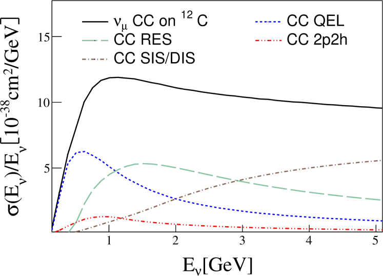
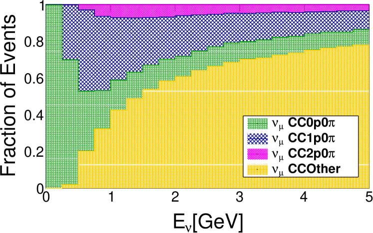
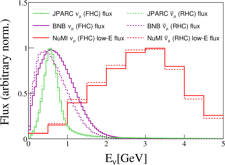
Figure 1: (Top) Summary of contributions from each interaction process to the CC $\nu_{\mu}$ cross section on ¹²C as a function of neutrino energy, $E_{\nu}$. (Middle) The corresponding fraction of the total $\nu_{\mu}$-¹²C events arising from each of the $0\pi$ topologies. This plot assumes a momentum threshold for protons of $450$ MeV/c while the GENIE predictions are obtained with the G18_10a_02_11b tune. (Bottom) Summary of $\nu_{\mu}$ (continuous lines) and $\overline{\nu}_{\mu}$ (dashed lines) normalized flux distributions for T2K ND280 at JPARC [6], MiniBooNE and MicroBooNE with the BNB [7], and MINER$\nu$A with the NuMI [8]. The flux predictions for neutrino and antineutrino modes are refereed to as “FHC” and “RHC,” respectively.

The GENIE Collaboration is building a global analysis of the neutrino, charged-lepton and hadron-scattering data. This comprehensive analysis of the world’s lepton-nuclear scattering data is being constructed in a staged manner, with recent efforts focused initially on the analysis of neutrino scattering on hydrogen and deuterium for the purpose of tuning aspects of the GENIE framework associated with the free-nucleon cross section: namely the SIS region [5] as well as tuning of hadronic multiplicities relevant for neutrino-induced hadronization models [9]. The present work extends this analysis campaign to a second stage: an explicit tune of nuclear model parameters to recent nuclear data.

This work is further necessitated by outstanding discrepancies between GENIE predictions and more recent datasets, which use heavy nuclei as targets. Several neutrino collaborations, such as MicroBooNE and MINER$\nu$A, tried to address these discrepancies by tuning GENIE against the $\nu_{\mu}$CC$0\pi$ T2K and inclusive $\nu_{\mu}$ CC MINER$\nu$A datasets, respectively [10, 11, 12]. All these tunes simulate 2p2h interactions with the Valencia model [13]. In both cases, the results suggest an enhancement of the 2p2h cross section. These tunes are not available for wider use within GENIE, and in some cases, these were performed with obsolete GENIE versions which differ substantially from the latest one.

In this paper, we describe the GENIE analysis of the available $\nu_{\mu}$ and $\overline{\nu}_{\mu}$ CC0$\pi$ datasets from MiniBooNE, T2K, MINER$\nu$A and MicroBooNE. The main goal is to provide improved simulations tuned to nuclear data and quantify the major sources of uncertainties in CC0$\pi$ measurements. In order to do so, new degrees of freedom are developed within the GENIE Monte Carlo (MC) event generator in order to quantify the effect of variation away from the nominal models. Most of the new degrees of freedom can be used to tune other available Comprehensive Model Configurations (CMCs) in GENIE. In this analysis we focus on the ‘retuning’ of the G18_10a_02_11b tune against $\nu_{\mu}$-¹²C CC0$\pi$ data from MiniBooNE, T2K and MINER$\nu$A. The G18_10a_02_11b was previously tuned against free-nucleon data [5]. In this paper, we refer to G18_10a_02_11b as the nominal tune.

All predictions shown in this paper are calculated using the G18_10a_02_11b tune. G18_10a_02_11b uses the Valencia model to simulate QEL and 2p2h events in the nuclear medium, while FSIs are modeled using the hA model and the nuclear ground state is described with the Local Fermi Gas (LFG) model [14]. The other interaction processes are common with the free-nucleon recipe described in Ref. [5]. Tab. 1 details the full list of interaction processes associated with this Comprehensive Model Configuration (CMC).

Simulation domain	Model
Nuclear model	Local Fermi Gas [14]
QEL and 2p2h	Valencia [13, 15]
QEL Charm	Kovalenko [16]
QEL $\Delta S=1$	Pais [17]
RES	Berger-Sehgal [18]
SIS/DIS	Bodek-Yang [19]
DIS $\Delta S=1$	Aivazis-Tung-Olness [20]
Coherent $\pi$ production	Berger-Sehgal [18]
Hadronization	AGKY [21]
FSI	INTRANUKE hA [22]

Table 1: Complete list of models used for the G18_10a_02_11a tune in GENIE v3 [5].

We stress that G18_10a_02_11b is only one of many CMCs that can be tuned within GENIE. Our main motivations behind this particular choice are: (1) we can use data-driven constraints from previous GENIE tunes on hydrogen and deuterium [5]; (2) the QEL and 2p2h processes are modeled with the Valencia model, a theory-based model which is used in most neutrino analyses; (3) FSI interactions are modeled with the INTRANUKE hA model, which is an easily tuned empirical model closely driven by hadron-nucleus scattering data. Other CMCs will be considered in future iterations of this work.

The GENIE global analysis software [5] is used to perform a partial tune for each experiment using double-differential flux-integrated CC0$\pi$ cross-section measurements as a function of muon kinematics. We further note that only carbon datasets are considered in this work. While a more expansive study of the nuclear $A$ dependence will be a valuable aspect of future work, this choice carries the advantage of providing a consistent basis for the exploration of statistical tensions. This work is a step closer to a global tune with neutrino-nucleus cross-section data, which can be performed using the same analysis strategy once all the tensions are well understood. Future iterations of this work will also incorporate measurements on different topologies, such as CC1$\pi^{\pm}$.

This work is organized as follows: Sec. II provides an overview of the available CC0$\pi$ data to date. The newly developed GENIE parameters are discussed in Sec. III. This is followed by a description of the tuning procedure in Sec. IV and a discussion of the tune results and tensions between CC0$\pi$ and CCNp0$\pi$ datasets in Sec. V. In addition, Sec. VI describes some modelling aspects relevant for the exploration of the CC0$\pi$ and CCNp0$\pi$ tension. The main conclusions of this paper are highlighted in Sec. VII.

II Review of neutrino nucleus CC0$\pi$ measurements

Cross-section measurements of the CC0$\pi$ topology were carried out by SciBooNE [23], NOMAD [24], MiniBooNE [25, 26], T2K ND280 [27], MINER$\nu$A [28, 29, 30] and MicroBooNE [31, 32]. This section provides with a review of neutrino-nucleus CC0$\pi$ data available to date.

II.1 Scattering topologies and kinematics of experimental data

The CC0$\pi$ topology is usually defined as a CC event with no pions in the final state, regardless of the number of protons in the event. However, the CC0$\pi$ topology definition is not universal as it varies between the different published measurements as a consequence of the different detection capabilities of each experiment. In some analyses, its definition is optimized to study more exclusive final states with a specific proton multiplicity. The following nomenclature is adopted to avoid confusion for the reader: analyses requiring one or more protons in the final state are referred to as CCNp0$\pi$, where $\mathrm{N}\!\geq\!1$. If the analysis requires exactly zero or one proton in the final state, N is the replaced by the corresponding number, i.e. CC0p0$\pi$ or CC1p0$\pi$, respectively, for events with either no visible protons or precisely one. In some cases, the topology definition requires at least two protons in the final state. This is denoted as CC2p0$\pi$. We note that, in this case, CC2p0$\pi$ events include the very small probability to have N$>\!2$ final-state protons — a scenario which is challenging to isolate experimentally. When there is no requirement on the proton multiplicity, the topology is refereed to as CC0$\pi$. Fig. 1 presents the fraction of $\nu_{\mu}$ CC events as a function of the neutrino energy for different CC topologies. In this particular plot, the CC0$\pi$ topology contribution is broken down into more exclusive topologies depending on the proton multiplicity. It can be concluded that CC0$\pi$ events dominate the event rate for $E_{\nu}<1.5$ GeV. At higher energies, the contribution from events with pions in the final state (CC other) dominates.

Tab. 2 lists the available CC0$\pi$ and CCNp0$\pi$ cross section measurements to date. The table summarizes the information of interest for the evaluation of the GENIE predictions: the target type, neutrino flux mean energy and event topology definition. The neutrino flux spectrum associated with each experiment is provided in Fig. 1 (bottom) [6, 7, 8]. We use the same neutrino flux prediction for MiniBooNE and MicroBooNE.

The kinematic quantity column in Tab. 2 lists the kinematic quantities used to extract the cross-section measurements. The definition of each kinematic quantity is given in Appendix  A. Some of the available measurements are double-differential or triple-differential ones. This is indicated by a comma-separated list for the kinematic quantities used in the corresponding analysis. In addition, the year of the data release and the number of bins ($N_{\text{Bins}}$) for each dataset are specified. The details on the analysis requirements for MiniBooNE, T2K ND280, MINER$\nu$A and MicroBooNE datasets as well as comparisons of the G18_10_02_11b predictions to the data are presented in Appendix B. The main observations from Appendix B are summarized in Sec. II.2. For completeness, Tab. 2 includes measurements from SciBooNE and NOMAD which are not discussed further in this paper as their analysis strategy is limited with respect to the other measurements discussed in this work.

Experiment	$\langle E_{\nu}\rangle$	Target	Topology	Kinematic quantity	$N_{\text{Bins}}$	Year	Ref.
$\nu_{\mu}$-A measurements
SciBooNE	700 MeV	12C	CC0$\pi$	$E_{\nu}^{\text{QEL}}$	5	2006	[23]	✕
NOMAD	23 GeV	12C	CC0$\pi$	$E_{\nu}^{\text{QEL}}$	10	2009	[24]	✕
MiniBooNE	$788$ MeV	12C	CC0$\pi$	$T_{\mu}$, $\cos\theta_{\mu}$	137	2010	[25]	✓
				$Q^{2}_{\text{QEL}}$	17
				$E_{\nu}^{\text{QEL}}$	14
T2K ND280	$600$ MeV	12C	CC0p0$\pi$	$p_{\mu}$, $\cos\theta_{\mu}$	60	2018	[27]	✓
	$600$ MeV	12C	CC1p0$\pi$	$\cos\theta_{\mu}$, $\cos\theta_{p}$, $p_{p}$	40	2018	[27]	✕
	$600$ MeV	12C	CC2p0$\pi$	$-$	1	2018	[27]	✕
	$600$ MeV	12C	CCNp0$\pi$	$\delta p_{T}$	8	2018	[27]	✕
				$\delta\phi_{T}$	8
				$\delta\alpha_{T}$	8
				$\Delta p_{p}$, $\cos\theta_{\mu}$, $p_{\mu}$	49
				$|\Delta\mathbf{p}_{p}|$, $\cos\theta_{\mu}$, $p_{\mu}$	49
				$\Delta\theta_{p}$, $\cos\theta_{\mu}$, $p_{\mu}$	35
MINER$\nu$A	$3.5$ GeV	12C	CC0$\pi$	$p^{\mu}_{T}$, $p^{\mu}_{L}$	144	2019	[28]	✓
				$Q^{2}_{\text{QEL}}$	16
				$E_{\nu}^{\text{QEL}}$	12
	$3.5$ GeV	12C	CCNp0$\pi$	$p_{p}$	25	2018	[29]	✓
				$\theta_{p}$	26
				$\delta p_{T}$	24
				$\delta\alpha_{T}$	12
				$\delta\phi_{T}$	18
	$3.5$ GeV	12C	CCNp0$\pi$	$\delta p_{Tx}$	32	2020	[30]	✕
				$\delta p_{Ty}$	33
	$6$ GeV	12C	CC0$\pi$	$p^{\mu}_{T}$, $p^{\mu}_{L}$	184	2020	[33]	✕
				$Q^{2}_{\text{QEL}}$	19
	$6$ GeV	12C	CCN0$\pi$	$p^{\mu}_{T}$, $p^{\mu}_{L}$, $\sum T_{p}$	660	2022	[34]	✕
				$E_{\mu}$, $q_{0}^{\text{QEL}}$, $\sum T_{p}$	540
MicroBooNE	$800$ MeV	40Ar	CC1p$0\pi$	$p_{\mu}$	7	2020	[31]	✕
				$\cos\theta_{\mu}$	7
				$p_{p}$	7
				$Q^{2}_{\text{QEL}}$	7
				$E_{\nu}^{\text{cal}}$	7
	$800$ MeV	40Ar	CCNp$0\pi$	$p_{\mu}^{\text{reco}}$	10	2020	[32]	✕
				$\cos\theta_{\mu}^{\text{reco}}$	12
				$p_{p}^{\text{reco}}$	10
				$\cos\theta_{p}^{\text{reco}}$	9
				$\theta_{\mu p}^{\text{reco}}$	6
$\overline{\nu}_{\mu}$-A measurements
NOMAD	$23$ GeV	12C	CC0$\pi$	$E_{\nu}^{\text{QEL}}$	6	2009	[24]	✕
MiniBooNE	$665$ MeV	12C	CC0$\pi$	$T_{\mu}$, $\cos\theta_{\mu}$	78	2013	[26]	✓
				$Q^{2}_{\text{QEL}}$	16
				$E_{\nu}^{\text{QEL}}$	14
T2K ND280	600 MeV	H2O	CC0$\pi$	$p_{\mu}$, $\cos\theta_{\mu}$	19	2019	[35]	✕
T2K ND280	600 MeV	12C	CC0$\pi$	$p_{\mu}$, $\cos\theta_{\mu}$	57	2020	[36]	✕
T2K WAGASCI	860 MeV	H20	CC0p0$\pi$	$\theta_{\mu}$	6	2021	[37]	✕
	860 MeV	CH	CC0p0$\pi$	$\theta_{\mu}$	6	2021	[37]	✕
MINER$\nu$A	$3.5$ GeV	12C	CC0p0$\pi$	$p^{\mu}_{T}$, $p^{\mu}_{L}$	60	2018	[38]	✓
				$Q^{2}_{\text{QEL}}$	8
				$E^{\text{QEL}}_{\nu}$	10

Table 2: Summary of CC0$\pi$ analyses of $\nu_{\mu}$ and $\overline{\nu}_{\mu}$ interactions on nuclei. For each analysis, information on the neutrino flux mean energy, target type and event topology is provided. The kinematic quantity column specifies the list of kinematic quantities used in the cross-section measurement. Integrated cross-section measurements are denoted with a “$-$”. All kinematic quantities are defined in Appendix. A. The last column specifies whether the dataset is considered in the analysis.

There is a now large body of CC0$\pi$ data in the literature. This work focuses on the tuning of double differential flux-integrated CC0$\pi$ and CC0p0$\pi$ cross-section measurements on carbon from MiniBooNE, T2K ND280 and MINER$\nu$A. This is sufficient for an initial study. Additional single- and triple-differential CCNp0$\pi$ datasets are not considered in the first iteration of this work; these will be included in future iterations. However, some comparisons are given in this paper.

It is important to note the differences between the measurements considered in this work. These are highlighted in Appendix B. A significant difference is the treatment of uncertainties. Bin-to-bin correlation are not reported by MiniBooNE for many of their cross section measurements (including the data used in this work). In addition, flux uncertainty is given as a single normalization uncertainty of 10.7% and 17.2% for neutrino and antineutrino measurements on carbon respectively. These treatments involve approximations from modern treatments and do not fully incorporate MiniBooNE uncertainties [39]. Despite the statistical limitations of this measurement, MiniBooNE’s datasets are included in the analysis for a complete study of CC0$\pi$ datasets on carbon. In this work, an additional normalization systematic uncertainty is added to account for the missing flux correlation, as suggested by Ref. [25].

II.2 Dataset overview and initial considerations

The need for a tuning exercise for GENIE is clear. A few comparisons of G18_10a_02_11b against the available nuclear data are shown here. The remaining plots are in Appendix A.

We observe in Figs. 2, 3 and 4 that CC0$\pi$ and CC0p0$\pi$ datasets are under-predicted, whilst the CCNp0$\pi$ datasets are in quite good agreement with the G18_10a_02_11b predictions. As a consequence, a coherent global tune of CC0$\pi$ and CCNp0$\pi$ datasets is not possible. Hence, the analysis is mostly focused on CC0$\pi$ and CC0p0$\pi$ datasets. Nonetheless, understanding the tension is essential for future tuning efforts. This tension is further explored in this paper.

MiniBooNE CC0$\pi$ (Fig. 2) and T2K ND280 CC0p0$\pi$ data are both under-predicted at muon backward angles, where the contribution to the prediction is mostly from CCQEL events. At forward angles, where the contribution from non-CCQEL events is significant, the data are also under-predicted. The disagreement with MINER$\nu$A CC0$\pi$ data are most significant in the region where 2p2h events dominate, $0.15<p_{T}<0.7$ GeV, see Fig. 3. Single-Transverse Kinematic Imbalance (STKI) variables [40] bring in new sensitivities and comparisons against MINER$\nu$A data are shown in Fig. 4. Non-QEL events and FSI contributions dominate the region of high $\delta p_{T}$ and $\delta\alpha_{T}$. These contributions are essential to describe the data.

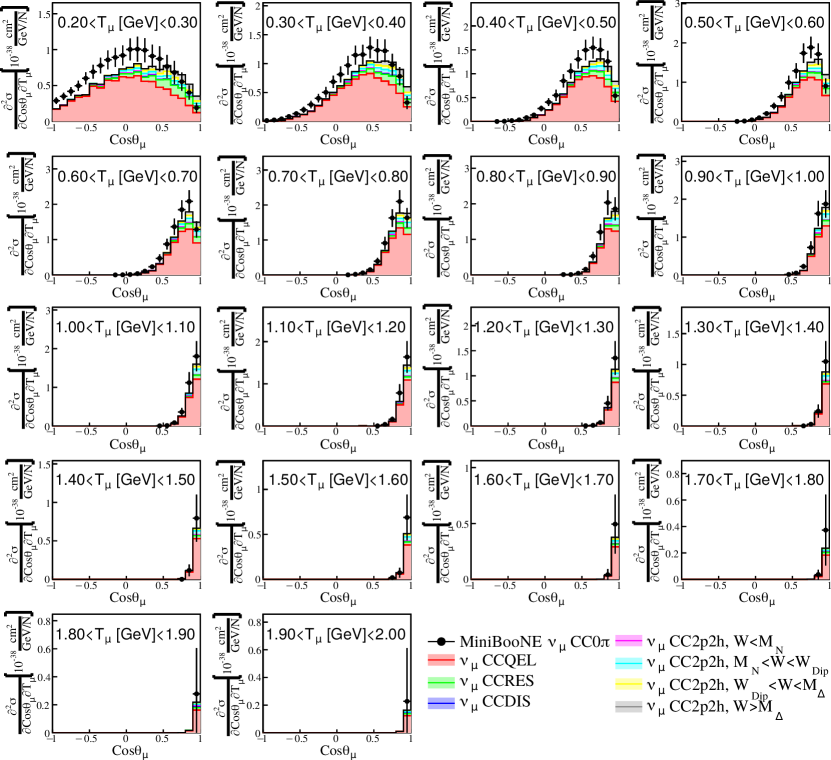
Figure 2: MiniBooNE $\nu_{\mu}$ CC0$\pi$ double differential flux-averaged cross section as a function of the muon angle ($\theta_{\mu}$) and kinetic energy ($T_{\mu}$) [25]. The corresponding slices on $T_{\mu}$ are compared against the G18_10a_02_11b tune. The GENIE prediction is divided into different interaction modes.

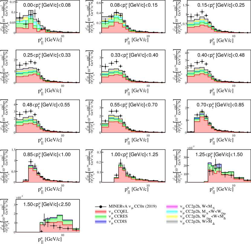
Figure 3: MINER$\nu$A $\nu_{\mu}$ CC0$\pi$ double differential flux-averaged cross-section as a function of the muon longitudinal momentum, $p_{\parallel}$, and transverse momentum, $p_{T}$ [28]. The corresponding slices on $p_{T}$ are compared against the G18_10a_02_11b tune. The GENIE prediction is divided into different interaction modes.

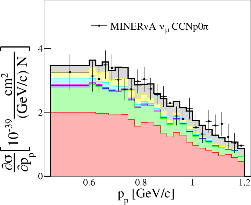
(a)

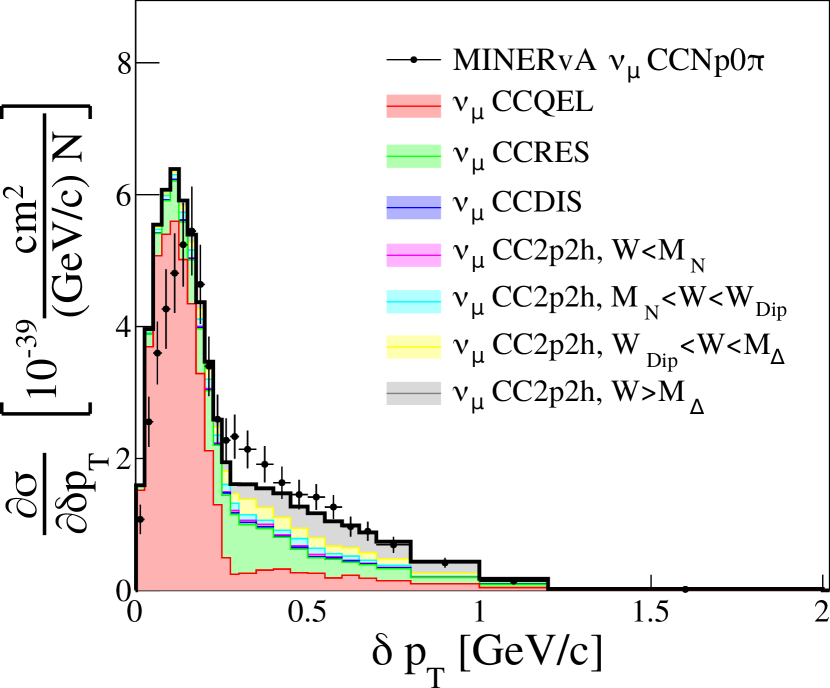
(b)

Figure 4: MINER$\nu$A $\nu_{\mu}$ CCNp0$\pi$ differential flux-averaged cross-section as a function of the leading-proton momentum, $\mathrm{p_{p}}$ (a), and the STKI variable [29, 30] $\delta\mathrm{p_{T}}$ (b). The data are compared against the G18_10a_02_11b tune. The GENIE prediction is divided into interaction modes.

The G18_10a_02_11b predictions as a function of the leading proton momentum show a dependency of 2p2h with $W$: at high proton momentum, 2p2h events with $W>M_{\Delta}=1232~{}\text{MeV}/\text{c}^{2}$ dominate, whilst the opposite is true at low momentum. This is highlighted in Fig. 4(a). 2p2h events contributing to the T2K ND280 CC0p0$\pi$ sample (Fig. 5) have $W<W_{\text{Dip}}=1120~{}\text{MeV}/\text{c}^{2}$. Higher multiplicity samples have a significant contribution from 2p2h events with $W>W_{\text{Dip}}$. The contribution from 2p2h events with $W<M_{N}=938~{}\text{MeV}/\text{c}^{2}$ is negligible for all the analyses discussed in this paper.

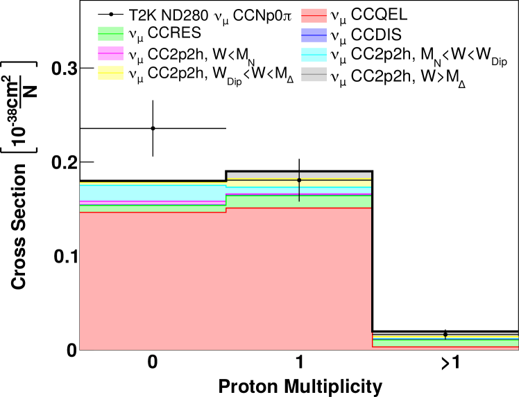
Figure 5: T2K ND280 flux-averaged $\nu_{\mu}$ CCNp0$\pi$ differential cross section as a function of the proton multiplicity [41]. The data are compared against the G18_10a_02_11b tune. The GENIE prediction is divided into different interaction modes.

For further comparisons to data, see Appendix B.

III Discussion of CC0$\pi$ model implementation in GENIE

This section describes the parameters available to most directly influence CC0$\pi$ predictions within G18_10a_02_11b. The parameters selected for this analysis are optimized for the G18_10a_02_11a tune. The complete list of parameters is shown in Tab. 3. The parameter ranges of interest used for the Professor parametrization are also provided. These can be grouped into five categories: CCQEL, CCSIS, CC2p2h, FSI or nuclear model parameters.

Not all the parameters from Tab. 3 have been included in the analysis presented in this paper. Only the parameters included in the final tune are described in this section. Other parameters of interest to tune CC0$\pi$ data that have been excluded from this analysis are described in Appendix. C. The reasons for excluding these parameters are summarized in Appendix C.3.

Most of these parameters can be applied to other CMCs [5]. We strive to have as many common, model-independent parameters to allow for systematic comparison between CMCs, but this is not always possible. An extension of this work to other CMC will be a subject of a future paper.

Parameter	Nominal Value	Range	In Final Tune
$M_{A}^{\text{QEL}}$ (GeV/c2)	$1.00\pm 0.01$	$[0.97,1.18]$	✓
$S_{\text{QEL}}$	$1$	$-$	✕
$\omega_{\text{RPA}}$	$1$	$[-0.5,1.5]$	✓
$\omega_{\text{No\,RPA}}$	$0$	$[-0.5,1.5]$	✓
$M_{A}^{\text{RES}}$ (GeV/c2)	$1.09\pm 0.014$	$-$	✕
$S_{\text{RES}}$	$0.84\pm 0.03$	$[0.5,1.5]$	✓
$R_{\nu p}^{\text{CC}1\pi}$	0.008	$-$	✕
$R_{\nu n}^{\text{CC}1\pi}$	$0.94\pm 0.075$	$-$	✕
$R_{\nu p}^{\text{CC}2\pi}$	$0.03\pm 0.01$	$-$	✕
$R_{\nu n}^{\text{CC}2\pi}$	$2.3\pm 0.12$	$-$	✕
$S_{N}^{\text{2p2h}}$	$1$	$[0,2]$	✓
$S_{\Delta}^{\text{2p2h}}$	$1$	$[0,2]$	✓
$S_{PL}^{\text{2p2h}}$	$1$	$[0,2]$	✓
$S_{Abs}^{\pi^{\pm}}$	$1$	$(1)$	✕
$S_{\text{MFP}}^{\pi^{\pm}}$	$1$	$(1)$	✕
$f^{\text{QEL}}$	$0$	$(0)$	✕
$f^{\text{2p2h}}$	$0$	$(0)$	✕

Table 3: Summary of parameters relevant for CC0$\pi$ analysis. The range of interest, nominal value in GENIE v3 is also shown. The range of interest corresponds to the parameter space used for the Professor parametrization [5]. ($-$) is used for parameters that are excluded in the analysis. The range for the parameters considered in the Professor parametrization but not used in the final tune is not reported. In such cases, the parameters are fixed to the corresponding nominal values (in parenthesis) in the final analysis, described in Sec. IV. The last column specifies whether the parameter is considered in the final analysis.

III.1 Charged-current quasi-elastic implementation

The QEL cross section at the free-nucleon level is parametrized with the QEL axial mass, $M_{A}^{\text{QEL}}$, and a QEL scaling factor, $S_{\text{QEL}}$. Both parameters are common in the simulation of neutrino interactions on free nucleons and nuclei. $M_{A}^{\text{QEL}}$ appears as the main degree of freedom in the widely-used dipole parametrization of the QEL form factor. We point out that more elaborate CMCs based on the z-expansion model [42] are now available in GENIE. In this work, preference is given to tune $M_{A}^{\text{QEL}}$ as hydrogen and deuterium data provide informative priors to help constrain this parameter [5].

The QEL cross section is affected by the dynamics of the nuclear medium. We include long-range nucleon-nucleon correlations in our calculations with the Random-Phase Approximation (RPA) correction [15]. The main effect of the RPA correction is a suppression of the QEL cross section at low $Q^{2}$. This correction is well supported by data and theory, but models differ in predicting its exact strength. This uncertainty is incorporated in GENIE with two parameters: one to scale the nominal QEL cross-section prediction with RPA corrections, $\omega_{\text{RPA}}$, and the other one to scale the QEL cross section without RPA corrections, $\omega_{\text{No\,RPA}}$. The total QEL cross section is calculated as a linear combination of the cross-section with and without RPA corrections:

$$\sigma^{\text{QEL}}=\omega_{\text{RPA}}\cdot\sigma^{\text{QEL}}_{\text{RPA}}+\omega_{\text{No\,RPA}}\cdot\sigma^{\text{QEL}}_{\text{No\,RPA}}.$$

This parametrization can be used to scale the QEL cross section when $\omega_{\text{RPA}}+\omega_{\text{No\,RPA}}\neq 1$. If $\omega_{\text{No\,RPA}}=0$, $\omega_{\text{RPA}}$ has the exact same effect as $S_{\text{QEL}}$. Therefore, $S_{\text{QEL}}$ is not included in the tune. One benefit of this approach is that possible scaling factors on the RPA parametrization do not alter the agreement with free-nucleon data. In addition, it reduces the analysis computing time. In Fig. 6, the CC QEL cross section as a function of the neutrino energy is shown for different combinations of $\omega_{\text{RPA}}$ and $\omega_{\text{No\,RPA}}$.

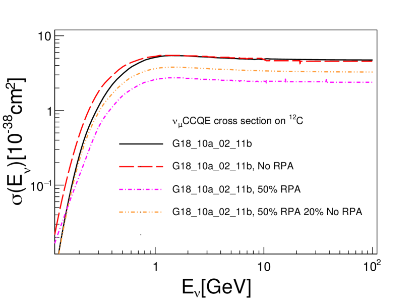
(a)

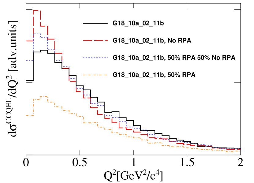
(b)

Figure 6: Impact of the RPA parametrization on the CCQEL cross section. The G18_10a_02_11b prediction is shown in black. The other predictions are obtained with the same tune while changing the RPA weight values. (a) Total CCQEL cross section for ¹²C. (b) Flux-integrated differential cross section as a function of $Q^{2}$. The prediction is obtained with the NuMI flux in low-energy mode.

Choosing each parameter range of interest is crucial for the correct evaluation of the post-fit uncertainties. In some cases, such as for $\omega_{\text{No\,RPA}}$, we sample negative values to allow the best-fit result to be at its physical limit of 0. In the case of the RPA parametrization, we impose the additional condition that $0.4<\omega_{\text{RPA}}+\omega_{\text{No\,RPA}}<1.6$ in the sampling on the phase space so that $\sigma^{\text{QEL}}>0$. Fig. 7 shows the distribution of sampled parameter values for $\omega_{\text{RPA}}$ and $\omega_{\text{No\,RPA}}$. Notice that the two limit cases are at the centre of the phase space.

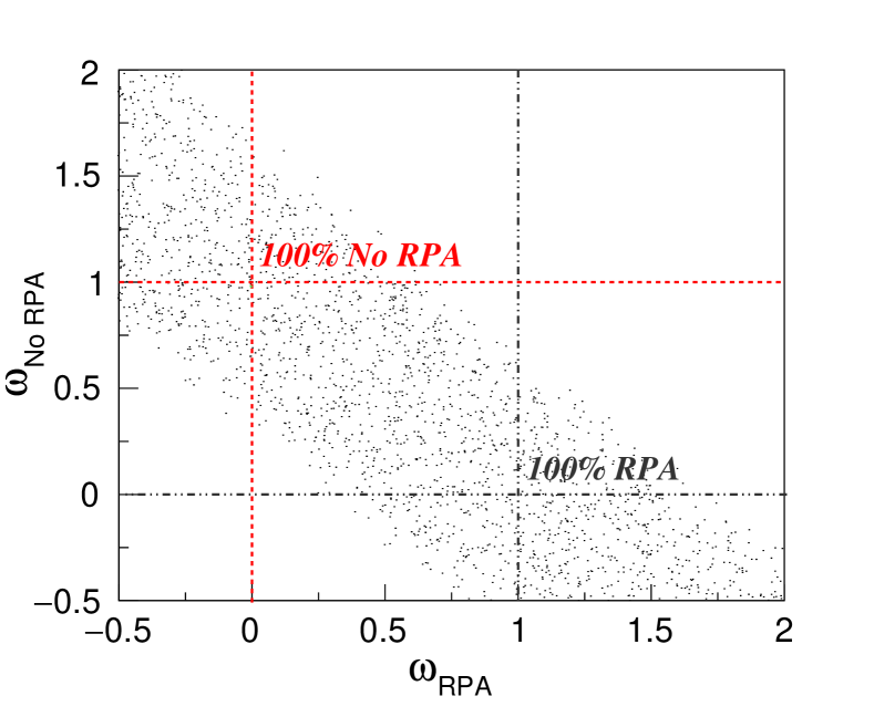
Figure 7: Distribution of scan points used for the GENIE tune in the $\omega_{\text{RPA}}$ vs $\omega_{No\,RPA}$ phase space. The grey (red) line intersection highlights the limit case in which we consider 100% (0%) of the RPA strength. This plot shows a total of 2,050 scan points distributed uniformly. The parameter ranges considered are those from Tab. 3.

It is desirable to apply priors to $\omega_{\text{RPA}}$ and $\omega_{\text{No\,RPA}}$, as effectively, parameter combinations for which $\mathcal{S}_{\text{RPA}}\equiv\omega_{\text{RPA}}+\omega_{\text{No\,RPA}}\neq 1$ act as a scaling of the QEL cross section. Hydrogen and deuterium QEL cross-section measurements are compatible with $\mathcal{S}_{\text{RPA}}=1$. However, nuclear effects might introduce an uncertainty in the scaling. A possible way to include this information is to consider uncorrelated priors on the sum, $\mathcal{S}_{\text{RPA}}$, and the difference, $\Delta_{\text{RPA}}\equiv\omega_{\text{RPA}}-\omega_{\text{No\,RPA}}$,

$$\mathcal{S}_{\text{RPA}}= \ 1\pm\sigma_{\mathcal{S}},$$

$$\Delta_{\text{RPA}}= \ 1\pm\sigma_{\Delta},$$

with $\sigma_{\mathcal{S}}$ and $\sigma_{\Delta}$ being the variance associated with the priors on $\mathcal{S}_{\text{RPA}}$ and $\Delta_{\text{RPA}}$, respectively. In terms of $\omega_{\text{RPA}}$ and $\omega_{\text{No\,RPA}}$, this approach includes a correlation between these parameters:

$$\Sigma_{\text{RPA}}=\frac{1}{4}\begin{pmatrix}\sigma_{\mathcal{S}}^{2}+\sigma_{\Delta}^{2}&\sigma_{\mathcal{S}}^{2}-\sigma_{\Delta}^{2}\\ \sigma_{\mathcal{S}}^{2}-\sigma_{\Delta}^{2}&\sigma_{\mathcal{S}}^{2}+\sigma_{\Delta}^{2}\\ \end{pmatrix}$$

This correlation between $\omega_{\text{RPA}}$ and $\omega_{\text{No\,RPA}}$ is included in the tune. The corresponding central values are $\mu_{\text{RPA}}=1$ and $\mu_{\text{No\,RPA}}=0$ respectively. The $\sigma_{\mathcal{S}}$ and $\sigma_{\Delta}$ are determined from previous tune iterations, see Sec. C.3. As concluded from Sec. II, some flexibility in the QEL scaling may be required to describe the data, hence, in this analysis $\sigma_{\mathcal{S}}=0.2$. This method requires that we impose a prior on $\Delta_{\text{RPA}}$ as well. Such prior affects the strength of the RPA correction, which we aim to constrain from data. In order to avoid strong constraints on $\Delta_{\text{RPA}}$, $\sigma_{\Delta}=5$.

Alternative parameterizations of the RPA correction uncertainty are available in the literature. Theory driven uncertainties specific for the Nieves model are estimated in Ref. [43]. Alternatively, T2K [12] and MicroBooNE [10] use empirical parameterizations to characterize the uncertainty on the RPA correction. For the first iteration of this work, we opted for a simple parameterization with two parameters to reduce the computational complexity of the tune.

Our method is similar to the RPA parametrization used in the latest theory-driven MicroBooNE tune [10]. The MicroBooNE Collaboration employed the GENIE ReWeight package to parametrize the RPA effect as a linear combination from the QEL cross section with the RPA correction to the QEL cross section without RPA using a single parameter limited to [0,1]. We refer to this tune as $\mu$BooNE tune. Both approaches are equivalent when $\mathcal{S}_{\text{RPA}}=1$.

III.2 Charged-current multi-nucleon implementation

The tuning of 2p2h models takes a central role in this work. As discussed in Sec. II, untuned GENIE CC0$\pi$ G18_10a_02_11b predictions underestimate the data in regions where 2p2h events contribute.

Previous tuning attempts by other neutrino collaborations indicate a preference for a higher 2p2h cross section. The simplest approach to enhance 2p2h is to use a global scaling factor. We refer to this parameter as $S_{\text{2p2h}}$. MINER$\nu$A opted for an empirical approach where they add an extra Gaussian contribution to enhance 2p2h interactions in $q_{0}$ and $q_{3}$. This is tuned to MINER$\nu$A CC inclusive data. This tune is known as MnvGENIE v1 tune [44, 45]. The $\mu$BooNE tune incorporates the 2p2h cross-section uncertainty with a linear extrapolation between the GENIE 2p2h Empirical and Valencia model to account for possible shape differences. In addition, $S_{\text{2p2h}}$ is also considered.

Different GENIE 2p2h models predict a slightly different strength and shape for the 2p2h cross section [46]. These differences motivated the development of a new parametrization that is able to modify the strength as well as the shape of the cross section in the $q_{0}$-$q_{3}$ space. This is accomplished by scaling the 2p2h differential cross section a function of $W$:

$$\frac{d^{2}\sigma^{\text{2p2h}}}{dq_{0}dq_{3}}\rightarrow S(W)\cdot\frac{d^{2}\sigma^{\text{2p2h}}}{dq_{0}dq_{3}}$$

$S(W)$ is the scaling function and $d^{2}\sigma^{\text{2p2h}}/dq_{0}dq_{3}$ the nominal double-differential cross section calculation.

The scaling function, $S(W)$, depends linearly on $W$. In this work, the scaling function is optimized for the Valencia model which has two characteristic peaks in the $q_{0}$-$q_{3}$ space, as it can be seen in Fig. 8. The peaks are situated at $W=M_{N}$ and $W=M_{\Delta}$. The dip between the two peaks is at $W_{\text{Dip}}$. This is implemented by imposing the following boundary conditions:

• $S_{PL,\min}^{\text{2p2h}}\equiv S(W=W_{PL,\min})$

• $S_{N}^{\text{2p2h}}\equiv S(W=M_{N})$

• $S_{\text{Dip}}^{\text{2p2h}}\equiv S(W=W_{\text{Dip}})$

• $S_{\Delta}^{\text{2p2h}}\equiv S(W=M_{\Delta})$

• $S_{PL,\max}^{\text{2p2h}}\equiv S(W=W_{PL,\max})$

The $S^{\text{2p2h}}$ parameters are referred to in this work as 2p2h scaling parameters. The limits of the 2p2h phase space are defined by $W_{PL,\min}$ and $W_{PL,\max}$. The upper limit is obtained by simply imposing $Q^{2}=0$. The lower limit is parametrized as a function of $q_{0}$ and $q_{3}$. This is an empirical approach that breaks the intrinsic microscopic model and it is only used to explore a possible dependency of the 2p2h cross section on $W$. In all GENIE v3 CMCs, the 2p2h scaling parameters are set to $1$.

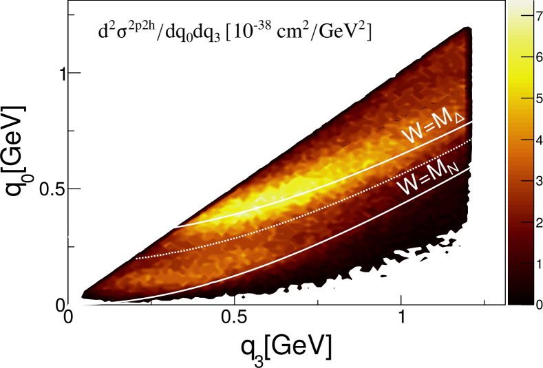
Figure 8: Double-differential $\nu_{\mu}$-¹²C CC2p2h cross section from the Valencia model in GENIE. Lines of constant $W$ at $W=M_{N}=938$ MeV/c², $W=M_{\text{Dip}}=1120$ MeV/c² (dotted line) and $W=M_{\Delta}=1232$ MeV/c² are also shown.

Only three out of the five 2p2h scaling parameters are included in the tune: $S^{\text{2p2h}}_{N}$, $S^{\text{2p2h}}_{\Delta}$ and $S^{\text{2p2h}}_{PL,\max}$. Events with $W<M_{N}$ are negligible for all CC0$\pi$ measurements of interest for this work, hence, $S^{\text{2p2h}}_{PL,\min}$ is not included in the tune. In addition, $S^{\text{2p2h}}_{\text{Dip}}$ is also not included as the region between $N$ and $\Delta$ peaks is too narrow in $W$ and the data cannot be sensitive to such parameter. In order to facilitate readability, the $S^{\text{2p2h}}_{PL,\max}$ parameter is redefined as $S^{\text{2p2h}}_{PL}$. In the particular case of T2K ND280, variations of $S_{\Delta}^{\text{2p2h}}$ and $S_{PL}^{\text{2p2h}}$ do not affect the CC0p0$\pi$ predictions. This is highlighted in Fig 5, where only events with $W<W_{\text{Dip}}$ contribute to the 2p2h cross section prediction with no protons above the detection threshold. Therefore, these parameters are not included when tuning against T2K ND280 CC0p0$\pi$ data.

The dependency of the scaling function with $W$ for a particular set of parameters is shown in Fig. 9 (top). This particular example enhances (suppresses) the 2p2h cross-section peak in the $W\!=\!M_{N}$ ($W\!=\!M_{\Delta}$) region. The example scaling function considers $S^{\text{2p2h}}(M_{N})\!=\!2$, $S^{\text{2p2h}}(M_{\Delta})\!=\!0.5$, and $S^{\text{2p2h}}(W_{PL,\min})\!=\!S^{\text{2p2h}}(W_{\text{Dip}})\!=\!S^{\text{2p2h}}(W_{PL,\max})\!=\!1$. The effect on the predictions of interest for this paper depends on the neutrino energy, proton multiplicity and proton momenta, as discussed in Sec. II.

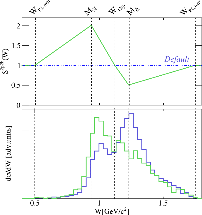
Figure 9: Graphic representation of the 2p2h scaling as a function of $W$. On the top, the default parametrization (dashed blue) and an example scaling function (green) are shown. The highlighted dashed vertical lines correspond to the tunable scaling parameters for $W=W_{PL}^{\min}$, $M_{N},\,W_{\text{Dip}}$, $M_{\Delta}$, and $W_{PL}^{\max}$. The bottom figure shows the Valencia 2p2h flux-integrated cross section as a function of $W$ for the G18_10a_02_11b tune in blue, and the same prediction scaled with the example scaling function in green. This plot is obtained simulating $\nu_{\mu}$ interactions on ¹²C with the NuMI $\nu_{\mu}$ low energy configuration [8].

III.3 Charged-current shallow-inelastic implementation

SIS events also contribute to the CC0$\pi$ signal as pions can be absorbed by the nuclear medium. Therefore, SIS mismodeling impacts the interpretation of the measurements and must be considered in the tune. The parameters available in GENIE to modify the RES and NRB background are:

1. RES axial mass, $M_{A}^{\text{RES}}$;

2. RES scaling factor, $S_{\text{RES}}$;

3. SIS scaling parameters that depend on the initial state, $R_{\nu p}^{\text{CC}1\pi}$, $R_{\nu n}^{\text{CC}1\pi}$, $R_{\nu p}^{\text{CC}2\pi}$, $R_{\nu n}^{\text{CC}2\pi}$.

These parameters have been previously tuned against hydrogen and deuterium data [5].

This is a lesser issue for MiniBooNE and T2K ND280 CC0$\pi$ data, more significant for the higher energy MINER$\nu$A data. Nuclear effects in SIS and DIS remain imperfectly understood and are therefore an important open area, both for the current study as well as future neutrino-nuclear interaction research. Nuclear-medium effects were studied for pion and electron beams [47] and found to be moderately significant.

The $S_{\text{RES}}$ parameter is the only SIS parameter included in the CC0$\pi$ tune. NRB parameters are not included: single pion NRB parameters have a small impact on the CC0$\pi$ predictions. In addition, higher multiplicity SIS/DIS contributions are negligible. In later instances, we refer to SIS/DIS contributions as DIS.

III.4 Discussion

The choice of tuning parameters is always complicated as these must sample the core physics dependencies with minimal correlation. In the $\mu$BooNE tune [10], only four parameters were used with an emphasis on RPA and 2p2h modeling. Although the RPA and 2p2h components are still important here, additional parameters are used to examine these aspects more fully. Since this exercise uses a broader range of neutrino energy, more parameters are needed to account for pion production. However, this contribution is small at neutrino energies $\sim$1 GeV and, although larger for MINER$\nu$A, we find that a single normalization parameter is sufficient to describe the CC0$\pi$ data included in this study. Additional potential parameters are introduced here and discussed more fully in Appendix C.

Similarly, as we discuss in more detail in Sec. IV.4, there can in principle be nonneglible correlations among the parameters associated with the nuclear models tuned in this current study and those associated with single-nucleon degrees of freedom as explored in Ref. [5]. A possible approach is to fit both sets of parameters comprehensively. In the present work we concentrate on a more targeted partial tune of these nuclear parameters in order to map their relationship to the corresponding data taken on nuclear targets. This is further justified by the fact that the leading sensitivity to the nuclear parameters is provided by the nuclear data fitted here. Ultimately, however, performing nuclear tunes with frozen single-nucleon parameters can be expected to influence the resulting nuclear tune through the correlations mentioned above; systematically disentangling these correlations will require a more global comprehensive tune involving simultaneous fits of both types of data, an undertaking which will be informed by the present study with respect to model priors, methodology, and an understanding of compatibility of nuclear data sets explored in partial tunes as discussed below.

In terms of specific nuclear model choices, the nuclear binding energy is a complicated topic that we quantify through a single number in existing GENIE models which is independent of the momentum distribution. This is adequate for inclusive electron scattering [48]. In more sophisticated treatments of semi-exclusive data, the binding energy and the missing momentum are interrelated via spectral functions [49]. Any binding energy parameters are found to be highly correlated with the other parameters chosen for tuning. We choose to leave this out of the tuning procedure and show the effect of these parameters in Appendix C.

Similarly, FSI has been studied for many years and there are many disagreements about the proper treatment [50]. Although this is a natural aspect of a full tune, the CC0$\pi$ data are not particularly sensitive to this aspect; FSI parameters are most sensitive to CCNp0$\pi$ data. A global analysis of CC0$\pi$ and CCNp0$\pi$ is out of the scope of this analysis and it is left for future iterations of this work. We show some interesting CCNp0$\pi$ sensitivities in Appendix C.

IV Tuning procedure

This section summarizes the tuning procedure for the analysis. The main goal is to tune GENIE against MiniBooNE, T2K ND280 and MINER$\nu$A CC0$\pi$ data.

IV.1 Construction of the GENIE prediction

In order to build the prediction associated with each dataset specified in Sec. II, we generate $\nu_{\mu}$ and $\overline{\nu}_{\mu}$ CC events for the experiment target using the neutrino fluxes from Fig. 1. In this work, the events are generated with the G18_10a_02_11b tune [5].

To compute the prediction associated with the $i$th dataset, we generate $N^{\text{TOT}}_{i}$ events. Events that do not satisfy the corresponding selection criteria specified in Sec. II are rejected. The number of accepted events in the $j$th bin is $N^{i}_{j}(\bm{\theta})$. $\bm{\theta}$ is the vector of tunable parameters specified in Tab. 3.

We build the corresponding $n$-differential flux-integrated cross section prediction for a given set of observables, $O$, as

$$\left(\frac{\partial^{n}\sigma_{th}(\bm{\theta})}{\partial O^{n}}\right)^{i}_{j}= \ \frac{N^{i}_{j}(\bm{\theta})}{\Phi_{i}N^{\text{TOT}}_{i}\Delta O^{i}_{j}}$$

$$\ \times\int dE_{\nu}\frac{d\phi_{i}}{dE_{\nu}}\sum_{T_{i}}R_{T_{i}}\sigma_{T_{i}}(E_{\nu},\bm{\theta}),$$

where $\Phi_{i}$ is the integrated flux for the $i$th dataset, $\Delta O^{i}_{k}$ corresponds to the $j$th $n$-dimensional bin volume for the quantities used in the differential cross section calculation, and $d\phi/dE_{\nu}$ is the expected flux at a given neutrino energy. For a target mix, the averaged cross section is evaluated by summing over the nucleus type in the target mix, $T_{i}$. The ratio of a specific nucleus type with respect to the total nuclei is $R_{T_{i}}$ and $\sigma_{T_{i}}(E_{\nu})$ is the total cross section for a given nucleus type.

IV.2 Avoiding the Peele’s Pertinent Puzzle

The bin-to-bin covariance matrix provided by each experiment is considered in the evaluation of the $\chi^{2}$. The T2K ND280, MicroBooNE and MINER$\nu$A datasets have highly correlated bin-to-bin covariance matrices. Previous attempts to fit neutrino-nucleus data using the full covariance matrices result in a significant reduction of the cross section [51, 10, 52]. These results are not surprising in highly correlated bins ($\rho>60\%$) in the Gaussian approximation [53]. This is known as Peele’s Pertinent Puzzle (PPP) [54, 53].

To avoid PPP, we change our variables in order to reduce the correlation for the $i$th dataset using the following prescription:

$$Z_{j}^{i}\equiv\begin{cases}\sum\limits_{k}D^{i}_{k}&j=0,\\ \dfrac{D^{i}_{j}}{\sum\limits_{k}D^{i}_{k}}&0<j<N^{i}.\end{cases}$$

$D^{i}_{j}$ corresponds to the $i$th dataset mean value at the $j$th bin. The $j$th and $k$th indices run over the number of bins associated with the $i$th dataset. This is known as Norm-Shape (NS) transformation. After the NS transformation, the integral is moved into the first bin of the $i$th dataset, whilst the rest describes the shape distribution. This transformation is applied to both data and predictions.

The bin-to-bin covariance associated with the $i$th dataset, $\Sigma_{D}(\mathbf{D})^{i}_{jk}$, transforms as follows:

$$\Sigma_{NS}(\mathbf{Z})_{jk}^{i}\equiv\left[\left(\frac{d\mathbf{Z}}{d\mathbf{D}}\right)\Sigma_{D}(\mathbf{D})\left(\frac{d\mathbf{Z}}{d\mathbf{D}}\right)^{T}\right]^{i}_{jk},$$

where

$$\left(\frac{d\mathbf{Z}}{d\mathbf{D}}\right)_{ja}^{i} = \begin{cases}1&j=0\\ \dfrac{\delta_{ja}\left(\sum\limits_{k}D_{k}^{i}\right)-D_{j}^{i}}{\left(\sum\limits_{k}D_{k}^{i}\right)^{2}}&0<j<N_{i}.\end{cases}$$

After the NS transformation the relative uncertainties are constant when the normalization changes.

The same transformation is applied to the prediction mean values and covariance. Before the NS transformation, the prediction covariance only has diagonal elements. This is not true after the NS transformation. However, the off-diagonal elements on the prediction covariance are small and are neglected in this work. The prediction central values and errors after the NS transformation are denoted as $Y^{i}_{j}(\theta)$ and $\delta Y^{i}_{j}(\theta)$ respectively.

IV.3 Professor parametrization

Given that performing a multi-parameter brute-force scan is not feasible, we use Professor [55] to parametrize the behavior of our predicted cross section and error in each bin in the NS space. We refer to this quantities as $\tilde{Y}_{j}^{i}(\bm{\theta})$ and $\delta\tilde{Y}_{j}^{i}(\bm{\theta})$. In this particular tune, we opted for a fourth-order parametrization. This work, where originally eleven parameters were included in the analysis, requires a total of 2k event generations with $\mathbf{\theta}$ sampled across the ranges specified in Tab. 3. The accuracy of the parametrization is shown in Fig. 10. The distribution is centered at zero with a standard deviation of 0.05. This distribution is similar to previous GENIE tunes [5]. This parametrization is used for the estimation of the best-fit values by minimizing the $\chi^{2}$.

The accuracy of the parameterization can be improved by increasing the order of the polynomial. However, an increase in the order of the polynomial is computationally expensive. For instance, a fifth-order polynomial requires 6k generations. A fourth-order polynomial is enough to describe the MC response in this work.

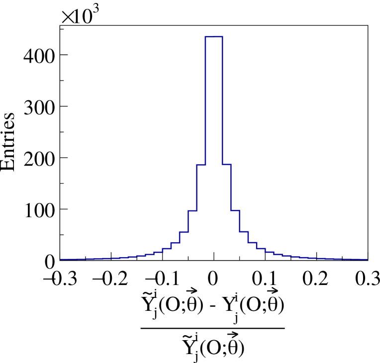
Figure 10: Fractional difference between true MC predictions in the NS space calculated with a given $\mathbf{\theta}$ parameter set.

IV.4 Discussion of data-driven priors

The basic structure of this tune is based on the model of separate nucleon and nucleus efforts. Although the emphasis here is on neutrino-nucleus parameters, some of the parameters of interest were already tuned to neutrino-nucleon data [5]. Particularly, the G18_10a_02_11b tune with hydrogen and deuterium data provided with data-driven constraints for $M_{A}^{\text{QEL}}$ and $S_{\text{RES}}$ [5]. These parameters are crucial for the description of free-nucleon data and are strongly correlated with other aspects of the nuclear tune. This correlation was observed in the $\mu$BooNE tune, leading to best-fit results with $M_{A}^{QE}=1.18\pm 0.08$ GeV/c² [10]. The effect of varying $M_{A}^{QEL}$ on the MINER$\nu$A $\nu_{\mu}$CC0$\pi$ prediction is shown in Fig. 11. In this work, we chose to constrain $M_{A}^{QEL}$ and $S_{RES}$ using data driven priors from Ref. [5]. The information on the parameter priors central values as well as the correlation between the two parameters out of the free-nucleon tune is included in the $\chi^{2}$ minimization. The complete information on the priors is provided in Tab. 4. In this analysis we also include priors on $\omega_{\text{RPA}}$ and $\omega_{\text{No\,RPA}}$, as discussed in Sec. III.1.

Parameter	Prior
$M_{A}^{\text{QEL}}$	$1.00\pm 0.01$ GeV/c2
$S_{\text{RES}}$	$0.84\pm 0.028$

(a)

	$M_{A}^{\text{QEL}}$	$S_{\text{RES}}$
$M_{A}^{\text{QEL}}$	$1.8\times 10^{-4}$	$1.5\times 10^{-4}$
$S_{\text{RES}}$	$1.5\times 10^{-4}$	$6.0\times 10^{-4}$

(b)

Table 4: Priors (a) and covariance matrix (b) for $M_{A}^{\text{QEL}}$ and $S_{\text{RES}}$ obtained to the free-nucleon tune from Ref. [5].

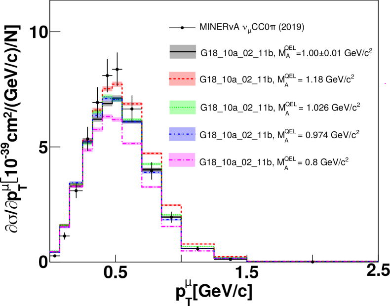
Figure 11: Impact of $M_{A}^{QEL}$ variations on MINER$\nu$A CC0$\pi$ flux-integrated differential cross section predictions as a function of $p_{T}$. The red line corresponds to the GENIE prediction computed with the $M_{A}^{QEL}$ best-fit value from the $\mu$BooNE tune [10]. No other parameters are modified from their nominal values.

IV.5 Evaluation of the $\chi^{2}$

The complete form for our $\chi^{2}$ is:

$$\chi^{2}(\bm{\theta})= \ \sum_{i}^{\mathcal{N}}\sum_{j,k}^{N_{i}}\sqrt{w^{i}_{j}}\Delta\tilde{Y}^{i}_{j}(\bm{\theta})(\Sigma_{NS,\,jk}^{i})^{-1}\Delta\tilde{Y}^{i}_{k}(\bm{\theta})\sqrt{w^{i}_{k}}$$

$$\ +\left(\bm{\theta}-\bm{\theta}_{0}\right)^{T}\Sigma^{-1}_{\theta}\left(\bm{\theta}-\bm{\theta}_{0}\right),$$ (1)

being $i$ the index that runs over the $\mathcal{N}$ datasets considered in the fit. $\Delta\tilde{Y}^{i}_{j}$ is the difference between the NS parametrization prediction and the $i$th dataset at the $j$th bin, $\Delta\tilde{Y}^{i}_{j}(\bm{\theta})\equiv\tilde{Y}^{i}_{j}(\bm{\theta})-Z^{i}_{j}$. The $\omega_{ij}$ is the weight applied to $j$th bin from the $i$th dataset. In this work, weights are used to include or exclude data from the analysis. In other words, they are either 1 or 0. The prediction errors, $\delta\tilde{Y}^{i}_{j}(\bm{\theta})$, are added in quadrature to $\Sigma_{NS}$. The second term takes care of correlated priors in our fit. $\bm{\theta}_{0}$ and $\Sigma_{\theta}$ are the central values vector and the covariance matrix of the priors for the parameters of interest. The details on the priors applied in this analysis are described in Sec. IV.4.

V Tuning Results

We adopt the following naming scheme to characterise each of the partial GENIE tunes presented in this work:

Gxx[a-d].

Here

• is a capital letter that stands for GENIE, highlighting the authorship of the tunes.

• is a number assigned to each experiment, i.e., MiniBooNE (10), T2K ND280 (20) or MINER$\nu$A (30). When using antineutrino datasets, xx is increased by one unit. For CCNp0$\pi$ datasets, xx is increased by five units.

• refers to the alternative intranuclear hadron model used in the analysis: (a) INTRANUKE/hA, (b) INTRANUKE/hN, (c) GEANT4/Bertini and (d) INCL++.

Note that this is different from the standard naming scheme used for the tunes released through the GENIE platform. The standard naming convention from Ref. [5] will be used if one or more of the tunes produced in this work or future iterations is prepared for release in GENIE.

In total, six partial tunes are performed: three tunes on neutrino CC0$\pi$ data, two tunes using antineutrino CC0$\pi$ data and one tune using $\nu_{\mu}$ CCNp0$\pi$ data. The tunes on CC0$\pi$ data aim to explore avenues for improving the agreement between GENIE and data, consolidate the main elements of the GENIE CC0$\pi$ tuning methodology and provide a common ground for the discussion of tensions. The tune on CCNp0$\pi$ data aims to highlight tensions between CC0$\pi$ and CCNp0$\pi$ datasets. All of the tunes presented in this work consider carbon datasets only. Joint fits to all available data will be performed at a future iteration of this work, aiming to produce the tunes that will be publicly released through the GENIE platform.

In all CC0$\pi$ tunes, the analyses are carried out using double-differential CC0$\pi$ data as a function of muon kinematics. Preference is given to datasets that do not require a minimum number of protons above detection threshold in the final state. Whenever CC0$\pi$ datasets are not available for a particular experiment, the tune is performed using CC0p0$\pi$ datasets instead.

G18_10a_02_11b is the starting point for all these tunes and provides the nominal predictions. The corresponding names assigned to each tune prepared for the purposes of this paper are the following:

• : GENIE tune to MiniBooNE $\nu_{\mu}$CC0$\pi$ data [25].

• : GENIE tune to MiniBooNE $\overline{\nu}_{\mu}$CC0$\pi$ data [26].

• : GENIE tune to T2K ND280 $\nu_{\mu}$CC0p0$\pi$ data [27].

• : GENIE tune to MINER$\nu$A $\nu_{\mu}$CC0$\pi$ data [28].

• : GENIE tune to MINER$\nu$A $\overline{\nu}_{\mu}$CC0p0$\pi$ data [38].

• : GENIE tune to MINER$\nu$A $\nu_{\mu}$CCNp0$\pi$ data [29].

Other measurements, including MicroBooNE ones, are used for comparisons only. Each partial tune is performed following the recipe described in Sec. IV.

V.1 Discussion of partial CC0$\pi$ tune results

Each tune’s best-fit parameter values and the $\chi^{2}$ calculated with the Professor parametrization at the best-fit point are summarized in Tab. 5. The nominal and best-fit predictions are shown in Figures 12, 13, 14, 15, 17, 16 and 18. Tab. 6 provides the $\chi^{2}$ values computed with each tune’s GENIE prediction and corresponding dataset. In this case, the $\chi^{2}$ values are calculated with the NS transformation with the GENIE predictions. Notice that the $\chi^{2}$ values from Tab. 6 are different to the ones provided in Tab. 5. This is a consequence of the Professor parametrization not being exact.

It is observed that the description of the data after the tune improved substantially. For instance, the agreement with MINER$\nu$A $\nu_{\mu}$ CC0$\pi$ before the tune is $\chi^{2}_{\text{Nominal}}=626/144$ DoF. After the tune, $\chi^{2}_{\text{Nominal}}=151/144$ DoF. This is mainly a consequence of an improvement in the overall normalization for each partial tune.

Parameters	G10a Tune	G11a Tune	G20a Tune	G30a Tune	G31a Tune	G35a Tune
$M_{A}^{\text{QEL}}$(GeV/c2)	$1.02\pm 0.01$	$1.01\pm 0.01$	$1.00\pm 0.01$	$1.00\pm 0.02$	$1.00\pm 0.01$	$0.99\pm 0.01$
$\omega_{\text{RPA}}$	$1.20\pm 0.03$	$1.14\pm 0.06$	$1.2\pm 0.2$	$0.9\pm 0.1$	$1.3\pm 0.2$	$0.75\pm 0.3$
$\omega_{\text{No\,RPA}}$	$0.05\pm 0.02$	$0.09\pm 0.05$	$-0.1\pm 0.1$	$0.2\pm 0.1$	$0.2\pm 0.2$	$0.09\pm 0.3$
$S_{\text{RES}}$	$0.85\pm 0.02$	$0.86\pm 0.05$	$0.84\pm 0.02$	$0.84\pm 0.03$	$0.84\pm 0.02$	$0.84\pm 0.02$
$S_{N}^{\text{2p2h}}$	$1.5\pm 0.4$	$2.3\pm 0.01$	$1.7\pm 0.3$	$1.2\pm 0.4$	$1.7\pm 0.5$	$0.33\pm 0.2$
$S_{\Delta}^{\text{2p2h}}$	$0.7\pm 0.2$	$0.7\pm 0.3$	(1.00)	$2.1\pm 0.2$	$2.3\pm 0.2$	$0.5\pm 0.4$
$S_{PL}^{\text{2p2h}}$	$0.4\pm 0.1$	$0.4\pm 0.1$	(1.00)	$0.9\pm 0.2$	$0.4\pm 0.1$	$1.5\pm 0.4$
$\chi^{2}$	89/130	77/71	60/55	61/137	67/53	17/19

Table 5: Best-fit parameter values for the different partial tunes. Parameter values within parenthesis are kept fixed during the fit. The $\chi^{2}$ values are calculated with the Professor parametrization, in accordance to Eq. 1.

Dataset	$\chi_{\text{Nominal}}^{2}$	$\chi_{\texttt{G10a}}^{2}$	$\chi_{\texttt{G11a}}^{2}$	$\chi_{\texttt{G20a}}^{2}$	$\chi_{\texttt{G30a}}^{2}$	$\chi_{\texttt{G31a}}^{2}$	$\chi_{\texttt{G35a}}^{2}$	DoF
MiniBooNE $\nu_{\mu}$ CC0$\pi$	1817	121	160	314	379	1279	2727	137
MiniBooNE $\overline{\nu}_{\mu}$ CC0$\pi$	444	208	214	246	403	491	879	60
T2K ND280 $\nu_{\mu}$ CC0p0$\pi$	139	447	600	123	237	916	239	60
MINER$\nu$A $\nu_{\mu}$ CC0$\pi$	626	252	202	270	151	360	953	144
MINER$\nu$A $\overline{\nu}_{\mu}$ CC0$\pi$	2259	1837	1680	2232	1794	82	1810	78

Table 6: Summary of $\chi^{2}$ values associated the CC0$\pi$ datasets specified in each row. The $\chi^{2}$ values are calculated using the NS method for seven different GENIE predictions: G18_10a_02_11b, G10a, G11a, G20a, G30a, G31a and G35a. The values highlighted in bold correspond to the best-fit $\chi^{2}$ for the partial tune predictions.

All carbon tunes show similar trends; whilst the tunes are in good agreement with the priors on $M_{A}^{\text{QEL}}$ and $S_{\text{RES}}$, the other parameters differ from the nominal parameter values. There is also a clear preference for QEL with RPA corrections. In addition, the tunes prefer a higher QEL, i.e. $\omega_{\text{RPA}}+\omega_{\text{RPA}}>1$, and 2p2h cross section. Finally, the different tunes suggest an underlying energy dependence on the 2p2h cross section strength and shape: the G10a, G11a and G20a tunes enhance (suppress) the Valencia 2p2h cross section at the nucleon ($\Delta$) region. Alternatively, the G30a and G31a tunes enhance the cross section at the nucleon and $\Delta$ region, with $S_{\Delta}^{2p2h}>S_{N}^{2p2h}$. A hint of an underlying energy dependence was also observed in Ref. [56].

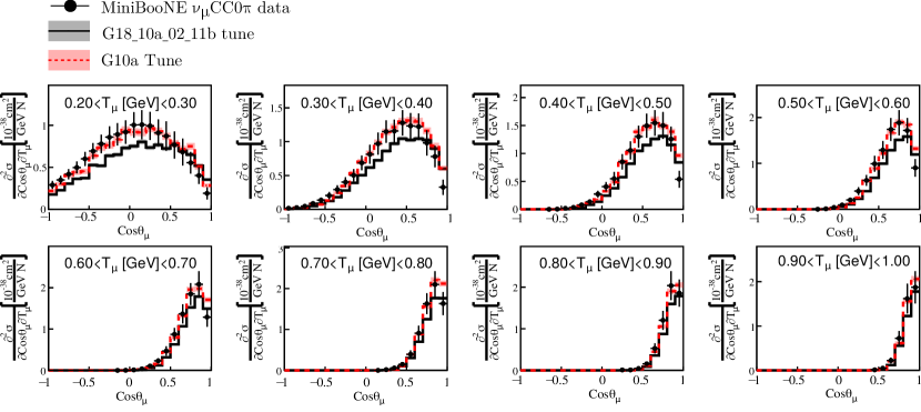
Figure 12: Comparison of the G18_10a_02_11b and G10a tunes against MiniBooNE $\nu_{\mu}$ CC0$\pi$ double differential data [25]. The comparisons are restricted to the $0.2<T_{\mu}<1.0$ GeV phase space. The predictions are computed using the parameters specified in Tab. 5. The total $\chi^{2}$ associated with this dataset before and after the tune are reported in Tab. 6.

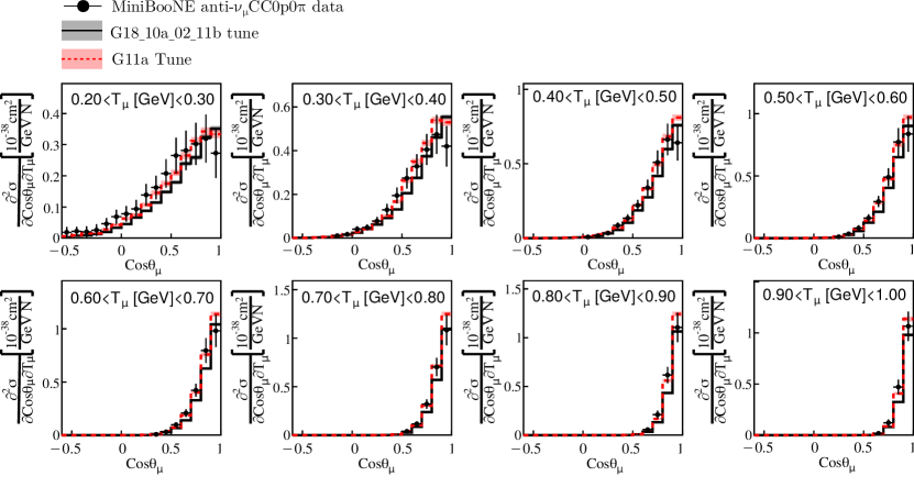
Figure 13: Comparison of the G18_10a_02_11b and G11a tunes against MiniBooNE $\overline{\nu}_{\mu}$ CC0$\pi$ double differential data [26]. The comparisons are restricted to the $0.2<T_{\mu}<1.0$ GeV phase space. The predictions are computed using the parameters specified in Tab. 5. The total $\chi^{2}$ associated with this dataset before and after the tune are reported in Tab. 6.

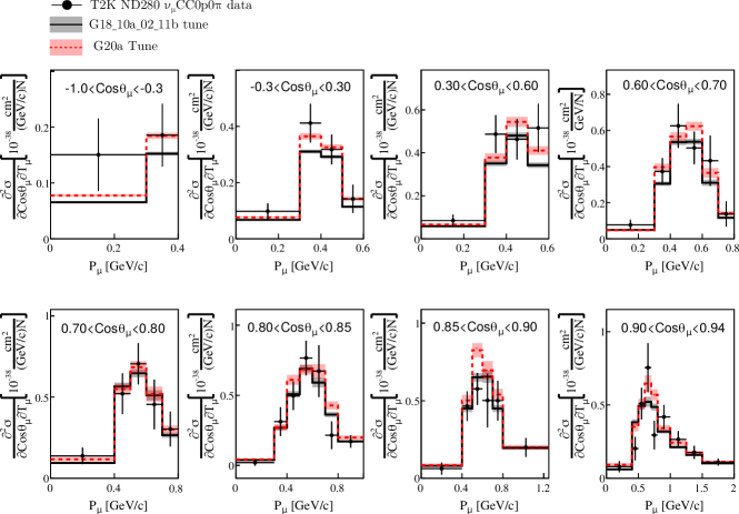
Figure 14: Comparison of the G18_10a_02_11b and G20a Tune against T2K ND280 $\nu_{\mu}$ CC0p0$\pi$ double differential data [27]. The comparisons are restricted to the $-1.0<\cos\theta_{\mu}<0.94$ phase space. The predictions are computed using the parameters specified in Tab. 5. The total $\chi^{2}$ associated with this dataset before and after the tune are reported in Tab. 6.

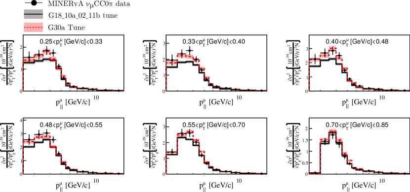
Figure 15: Comparison of the G18_10a_02_11b and G30a tunes against MINER$\nu$A $\nu_{\mu}$ CC0$\pi$ double differential data [28]. The comparisons are restricted to the $0.25<p_{T}<0.85$ GeV/c phase space. The predictions are computed using the parameters specified in Tab. 5. The total $\chi^{2}$ associated with this dataset before and after the tune are reported in Tab. 6.

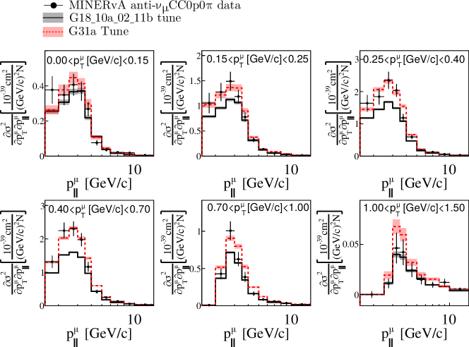
Figure 16: Comparison of the G18_10a_02_11b and G31a tunes against MINER$\nu$A $\overline{\nu}_{\mu}$ CC0p0$\pi$ double differential data [26]. The comparisons are restricted to the $0<p_{T}<1.5$ GeV/c phase space. The predictions are computed using the parameters specified in Tab. 5. The total $\chi^{2}$ associated with this dataset before (after) the tune reported in Tab. 6.

The enhancement of the QEL cross section is crucial for the description of MiniBooNE CC0$\pi$ data at $\cos\theta_{\mu}<0$. Particularly, the G10a and G11a tunes suggest an increase of the QEL cross section of about 20%. Similar QEL scalings have been observed by MicroBooNE [10] and recent Lattice Quantum-ChromoDynamics (QCD) calculations [57]. The increase (decrease) of the $S_{N}^{\text{2p2h}}$ ($S_{\Delta}^{\text{2p2h}}$ and $S_{PL}^{\text{2p2h}}$) is also crucial to correctly describe MiniBooNE $\nu_{\mu}$ and $\overline{\nu}_{\mu}$ CC0$\pi$ data.

The G20a tune also offers a better description of T2K ND280 CC0p0$\pi$ data. This tune suggests a scaling of $S_{N}^{\text{2p2h}}=1.7\pm 0.3$, compatible with the results presented by MicroBooNE [10]. In this particular case, the scaling of QEL is around 10%. The post-fit value of $\omega_{\text{No\,RPA}}$, although negative, is compatible with zero. This result is physical as $\omega_{\text{RPA}}+\omega_{\text{No\,RPA}}>0$, hence the total cross-section is positive. This scenario can be avoided by reducing the $\omega_{\text{No\,RPA}}$ range to [0,1.5]. However, the parameter range is not reduced further to allow a valid estimation of the error on $\omega_{\text{No\,RPA}}$.

Before the tune, the G18_10a_02_11b prediction under-predicted MINER$\nu$A CC0$\pi$ data in the phase-space regions where 2p2h events dominate ($0.15<p_{T}<0.7$ GeV/c). The results suggest that an enhancement of QEL, as well as 2p2h, improves the agreement with data. In fact, the G30a and G31a tunes provide with a better description of $\nu_{\mu}$ CC0$\pi$ and $\overline{\nu}_{\mu}$ CC0p0$\pi$ data respectively. The improvement in the normalization of the cross section is reflected in the post-fit $\chi^{2}$ values from Tab. 6. The same is true for the cross section as a function of the reconstructed neutrino energy, Fig. 18, and single-differential cross section data, Figs. 17 and 19. Both tunes over-predict the data at very low $Q^{2}_{\text{QEL}}$.

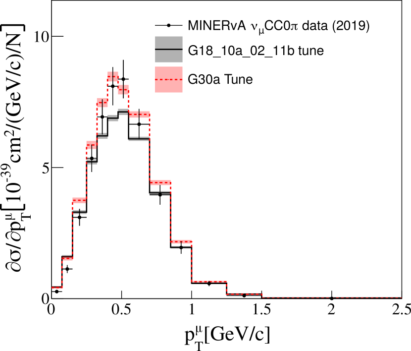
(a)

Figure 17: Comparison of the G18_10a_02_11b and G30a tunes against MINER$\nu$A $\nu_{\mu}$ CC0p0$\pi$ single-differential data [28]. The predictions are computed using the parameters specified in Tab. 5.

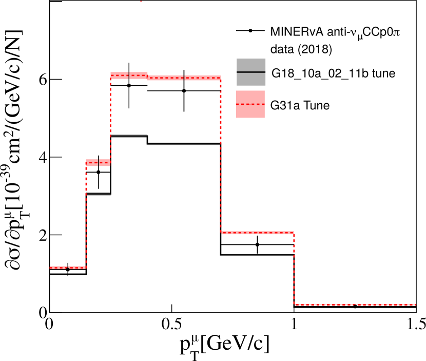
(a)

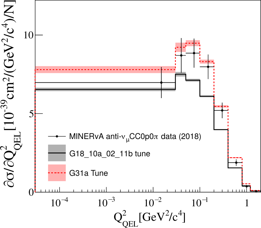
(b)

Figure 18: Comparison of the G18_10a_02_11b and G31a tunes against MINER$\nu$A $\overline{\nu}_{\mu}$ CC0p0$\pi$ single-differential data [26]. The predictions are computed using the parameters specified in Tab. 5.

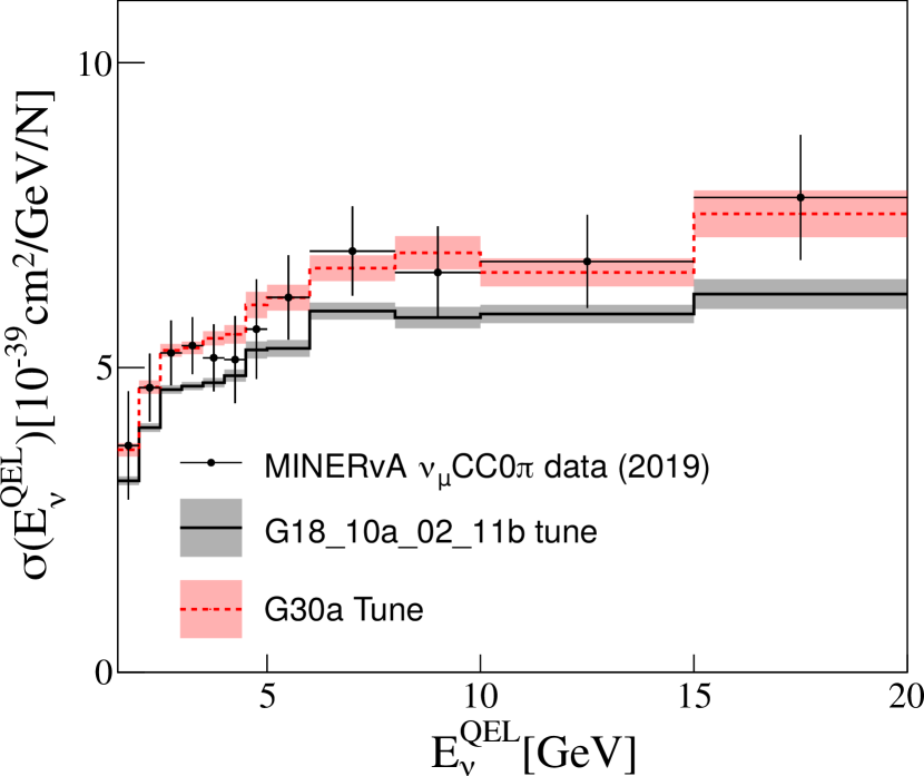
(a)

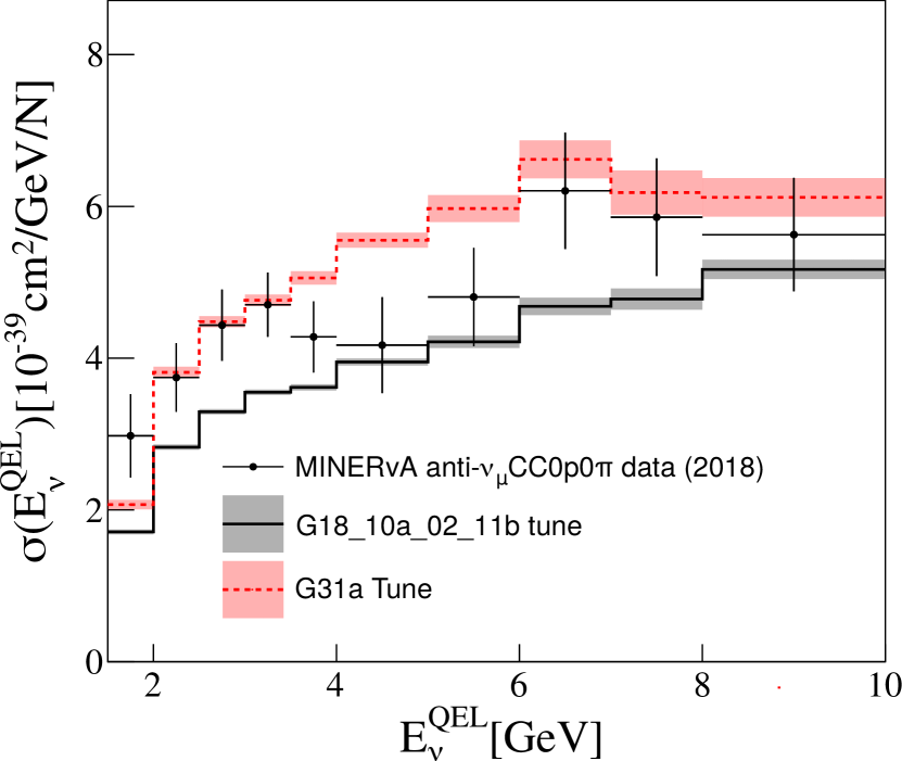
(b)

Figure 19: Comparison of G18_10a_02_11b, G31a (a) and G31a (b) against MINER$\nu$A $\nu_{\mu}$ and $\overline{\nu}_{\mu}$ CC0p0$\pi$ integrated cross section data [28, 26]. The predictions are computed using the parameters specified in Tab. 5.

V.2 Tension between CC0$\pi$ partial tunes

Tensions between datasets can be explored by comparing the different tunes. Figure 20 compares the G10a, G20a and G30a predictions against MiniBooNE $\nu_{\mu}$ CC0$\pi$ data. Even though the normalization of the three tunes is similar, differences in the predicted cross-section shape exist. The G10a tune is the only one out of the three that successfully describes the shape of the data, as it can be seen in Fig. 20 (left). The other tunes underestimate the cross-section at backward muon angles. In addition, the G30a Tune over-predicts the cross section at forward angles as a consequence of the enhancement of the 2p2h cross section at the $\Delta$-region. All tunes overestimate the cross section at forward muon angles and low muon kinetic energies, as demonstrated in Fig. 20 (right).

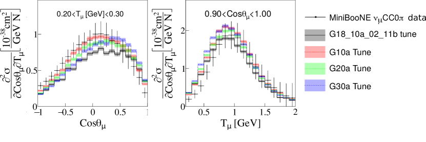
Figure 20: Comparison of the G18_10a_02_11b, G10a, G20a and G30a tunes against MiniBooNE $\nu_{\mu}$ CC0p0$\pi$ integrated cross-section data [25]. The predictions are computed using the parameters specified in Tab. 5.

The G31a tune is in clear tension with all the rest, including partial tunes performed with MINER$\nu$A neutrino data. In comparison with the rest of the tunes, the G31a tune prefers higher QEL and 2p2h cross sections. This leads to the over-prediction of all the other datasets. The comparison of G30a and G31a against MINER$\nu$A and MiniBooNE $\nu_{\mu}$ CC0$\pi$ data are shown in Fig. 21. The effect of this tension on the $\chi^{2}$ is reported in Tab. 6.

The tension between the G31a tune and the rest can have different origins. A possibility is that the model does not fully characterize the difference between neutrino and anti-neutrino fluxes. This is investigated comparing the G20a tune to the T2K WAGASCI antineutrino data. Both the T2K WAGASCI and T2K ND280 analysis explore the $\overline{\nu}_{\mu}$ CC0p$0\pi$ topology, but these are exposed to different neutrino fluxes (see Appendix. B.2). The impact of the G20a tune to these predictions is shown in Fig. 22. It is observed that the G20a tune has little impact on the T2K WAGASCI predictions. This indicates than an additional neutrino/antineutrino modeling uncertainty should be considered in a global tune of neutrino and antineutrino data. Another possible source of uncertainty is the different topology definition for MINER$\nu$A’s $\overline{\nu}_{\mu}$ dataset, with requires no visible protons above $T_{p}=120$ MeV for the antineutrino sample. The proton multiplicity uncertainty is explored further in Sec. V.3.

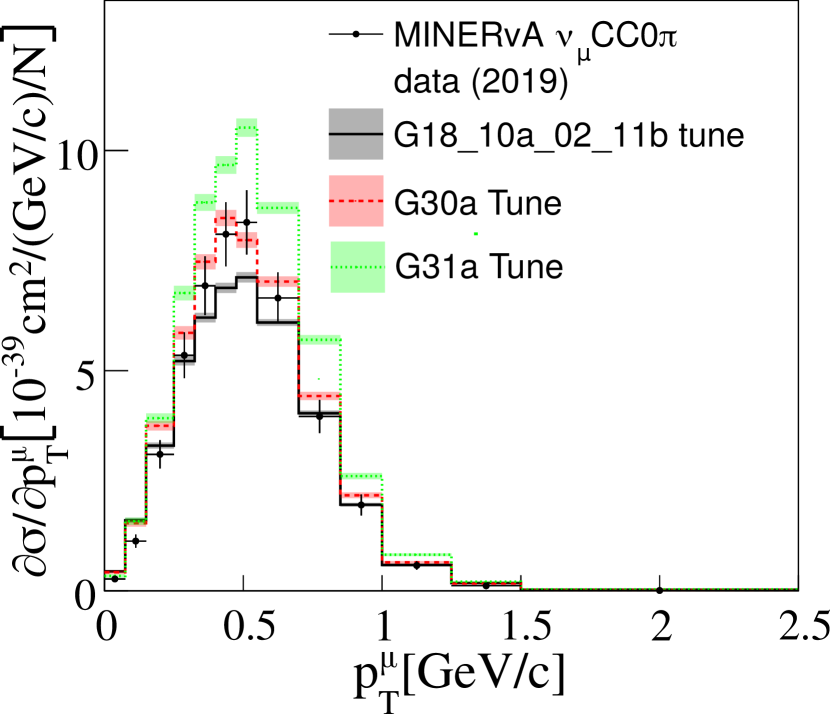
(a)

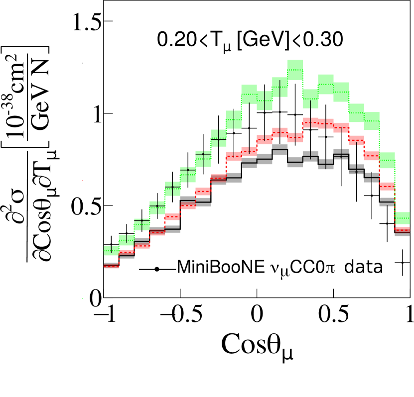
(b)

Figure 21: Comparison of the G18_10a_02_11b, G30a and G31a tunes against (a) MINER$\nu$A [28] and (b) MiniBooNE [25] $\nu_{\mu}$ CC0p0$\pi$ double-differential cross-section data. The predictions are computed using the parameters specified in Tab. 5.

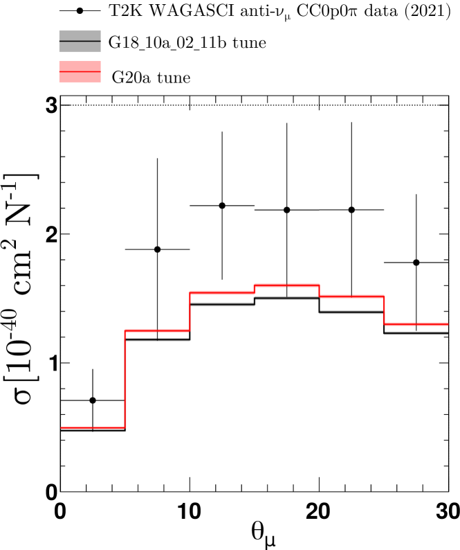
Figure 22: Comparison of the G18_10a_02_11b and G20a tunes against T2K WAGASCI $\overline{\nu}_{\mu}$ CC0p0$\pi$ data.

V.3 Tensions between $\nu_{\mu}$ CC0$\pi$ and $\nu_{\mu}$ CCNp0$\pi$ datasets

T2K ND280, MINER$\nu$A and MicroBooNE are the only experiments that released cross-section measurements for different proton multiplicities. As discussed in Sec. II.2, CC0$\pi$ and CC0p0$\pi$ datasets are under-predicted, whilst the CCNp0$\pi$ datasets are slightly over-predicted by the nominal G18_10a_02_11b prediction. This modeling limitation is also observed in Ref. [56, 58, 27].

After the partial tunes using $\nu_{\mu}$ CC0$\pi$ data, the agreement with CCNp0$\pi$ data deteriorates. This is highlighted in Tab. 7, which summarizes the post-fit $\chi^{2}$ values associated with CCNp0$\pi$ datasets. In all cases, the $\chi^{2}$ computed with each partial tune prediction increases with respect to the $\chi^{2}$ computed with the nominal G18_10a_02_11b tune.

Dataset	$\chi_{\text{Nominal}}^{2}$	$\chi_{\texttt{G10a}}^{2}$	$\chi_{\texttt{G11a}}^{2}$	$\chi_{\texttt{G20a}}^{2}$	$\chi_{\texttt{G30a}}^{2}$	$\chi_{\texttt{G31a}}^{2}$	$\chi_{\texttt{G35a}}^{2}$	DoF
T2K ND280 CCNp0$\pi$ data
$d\sigma/d\delta p_{T}$	228	1741	1499	883	759	95	25	8
$d\sigma/d\delta\phi_{T}$	292	2489	2117	1190	1049	1950	16	8
$d\sigma/d\delta\alpha_{T}$	27	58	53	42	41	95	21	8
MINER$\nu$A CCNp0$\pi$ data
$d\sigma/dp_{p}$	21	22	25	32	36	58	27	25
$d\sigma/d\theta_{p}$	58	153	150	113	129	226	20	26
$d\sigma/d\delta p_{T}$	102	637	568	360	352	625	42	24
$d\sigma/d\delta\phi_{T}$	87	505	467	314	354	566	18	23
$d\sigma/d\delta\alpha_{T}$	15	21	29	24	30	57	17	12
$d\sigma/d\delta p_{Tx}$	159	727	710	467	555	768	62	32
$d\sigma/d\delta p_{Ty}$	127	832	776	553	599	792	51	33
MicroBooNE CCNp0$\pi$ data
$d\sigma/dp_{\mu}^{\text{reco}}$	71	402	413	245	251	1186	40	10
$d\sigma/d\cos\theta_{\mu}^{\text{reco}}$	413	238	236	210	245	471	149	12
$d\sigma/dp_{p}^{\text{reco}}$	33	96	97	73	76	267	20	10
$d\sigma/d\cos\theta_{p}^{\text{reco}}$	100	176	179	135	139	393	33	9
$d\sigma/d\theta_{\mu p}^{\text{reco}}$	549	186	196	199	218	304	136	6

Table 7: Summary of $\chi^{2}$ values associated the CCNp0$\pi$ datasets specified in each row. The $\chi^{2}$ values are calculated using the NS method for seven different tunes: G18_10a_02_11b, G10a, G11a, G20a, G30a and G31a. The values highlighted in bold correspond to the best-fit $\chi^{2}_{\texttt{G35a}}$ for the partial tune using the specified dataset.

All G10a, G20a and G30a tunes overpredict $\nu_{\mu}$ CCNp0$\pi$ data. Figure 23 shows a comparison of the partial tune predictions against different single-differential CCNp0$\pi$ cross-section measurements from MINER$\nu$A. Figure 23 shows that none of the available tunes can describe the peak at low $\delta p_{T}$ and that all partial tunes overestimate the cross section at low proton momentum and forward angles. The same observations are made when comparing the tunes against T2K ND280 and MicroBooNE CCNp$0\pi$ data, see Figs. 24 and 25, respectively.

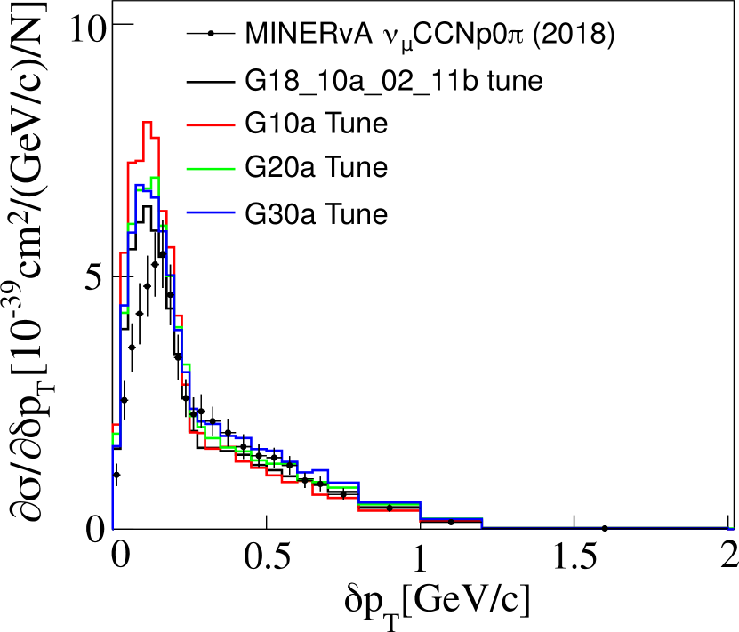
(a)

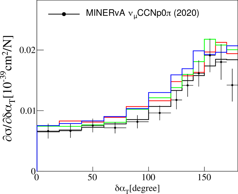
(b)

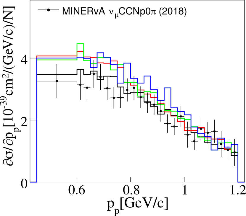
(c)

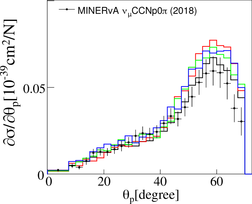
(d)

Figure 23: Comparison of the G18_10a_02_11b, G10a, G20a and G30a tunes against MINER$\nu$A $\nu_{\mu}$ CCNp0$\pi$ single-differential cross-section data as a function of (a) $\delta p_{T}$, (b) $\alpha_{p}$, (c) $p_{p}$ or (d) $\theta_{p}$. In order to ease the readability of these plots, no statistical errors are shown. The predictions are computed using the parameters specified in Tab. 5.

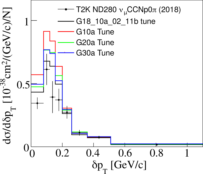
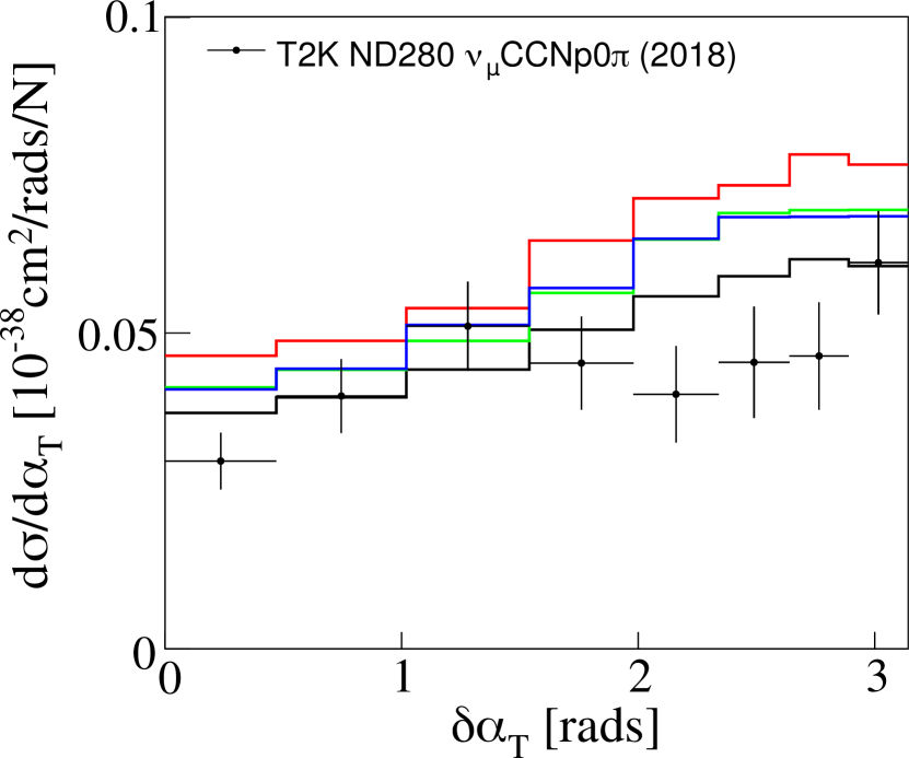
Figure 24: Comparison of the G18_10a_02_11b, G10a, G20a and G30a tunes against T2K ND280 $\nu_{\mu}$ CCNp0$\pi$ single-differential cross-section data as a function of (a) $\delta p_{T}$ or (b) $\delta\alpha_{T}$ [27]. In order to ease the readability of these plots, no statistical errors are shown. The predictions are computed using the parameters specified in Tab. 5.

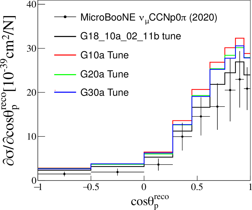
(a)

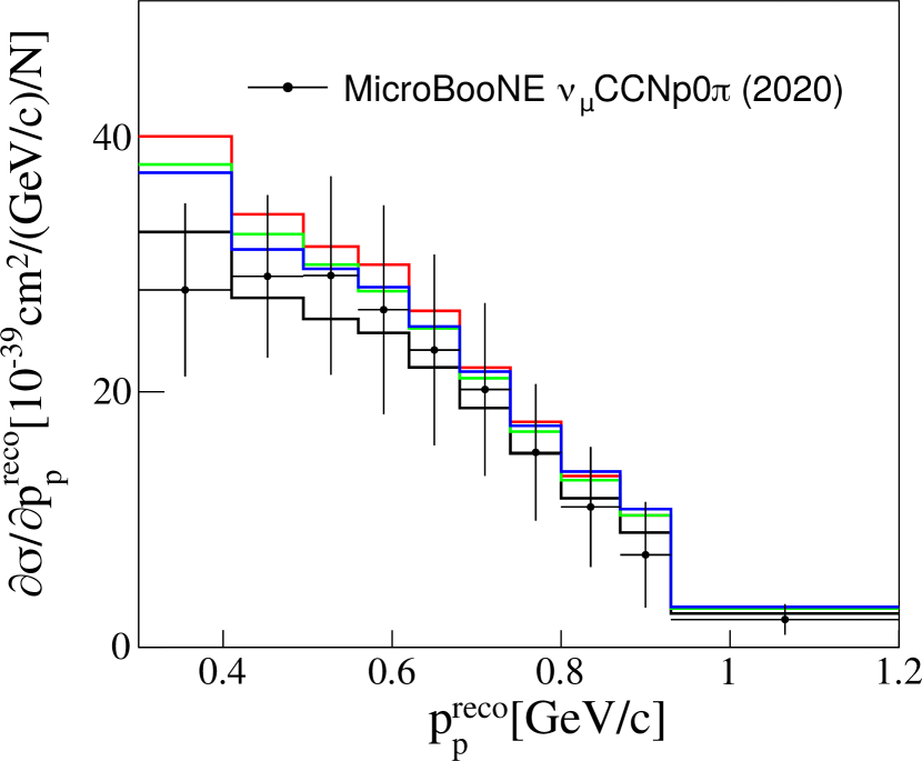
(b)

Figure 25: Comparison of the G18_10a_02_11b, G10a, G20a and G30a tunes against MicroBooNE $\nu_{\mu}$ CCNp0$\pi$ single-differential cross-section data as a function of (a) $\cos\theta_{p}^{\text{reco}}$ or (b) $p_{p}^{\text{reco}}$ [32]. In order to ease the readability of these plots, no statistical errors are shown. The predictions are computed using the parameters specified in Tab. 5.

To further explore this tension, an additional tune is performed using the MINER$\nu$A $\nu_{\mu}$ CCNp0$\pi$ dataset as a function of the proton angle. Following the naming scheme described at the beginning of Sec. V, this tune is referred to as G35a. The best-fit results are listed in Tab. 5.

The G35a tune suggests a significant reduction of the QEL cross section. In addition, the tune suppresses the Valencia cross-section peak prediction at $W=M_{N}$ and shifts the $\Delta$ peak to $W>M_{\Delta}$. This result contradicts the rest of the partial tunes presented in this article, reinforcing the fact that there is a strong tension between CC0$\pi$ and CCNp0$\pi$ datasets. The summary of $\chi^{2}$ is reported in Tab. 6 and Tab. 7.

An important observation is that the G35a tune also improves the agreement with MicroBooNE CCNp0$\pi$ data, suggesting that a possible A-dependency on the parameters does not play an important role.

The tension between CC0$\pi$ and CCNp0$\pi$ datasets needs to be resolved before attempting a global tune of CC0$\pi$ data that can describe all data available to date. Some modelling aspects that may contribute to this tension are investigated in Sec. VI.

VI Investigation of tensions between CC0$\pi$ and CCNp0$\pi$ datasets

This section offers an insight into possible modeling implementations that may contribute to the tension between CC0$\pi$ and CCNp0$\pi$ datasets and explores avenues of accommodating both within future joint tunes. None of the uncertainties described in this section has a big impact on CC0$\pi$ datasets.

VI.0.1 Nuclear model variations

The nuclear model determines the momentum and binding energy of the hit nucleon. In GENIE, three nuclear models are available: Relativistic Fermi Gas (RFG), Local Fermi Gas (LFG) and Correlated Fermi Gas (CFG) [14]. By default, G18_10a_02_11b uses the LFG.

The nuclear model choice affects the CCNp0$\pi$ predictions. Figure 26 shows the impact of the underlying nuclear model against CCNp0$\pi$ single-differential cross-section measurements as a function of $\delta p_{T}$. Differences between the models are significant for the cross-section peak prediction at low $p_{T}$. The RFG model is the only one out of the three that predicts the MINER$\nu$A data below the maximum. However, it still over-predicts the cross section at the peak. Alternatively, the CFG model successfully predicts the peak normalization. This is reflected in the $\chi^{2}_{\text{CFG}}$, reported in Tab. 8.

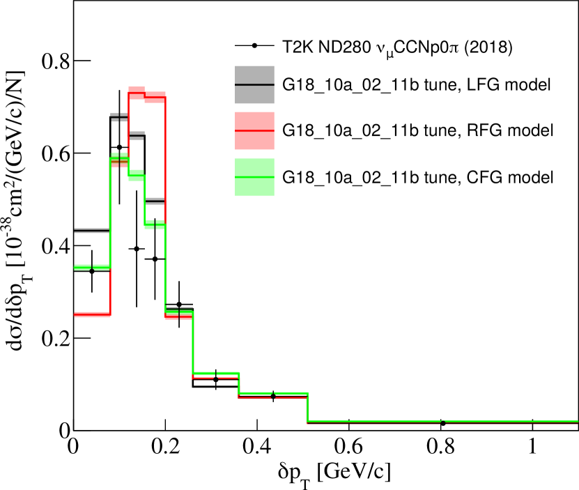
(a)

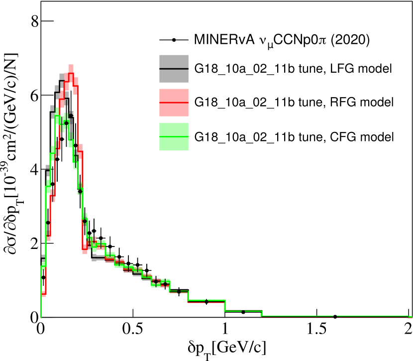
(b)

Figure 26: Comparison of the G18_10a_02_11b tune against T2K ND280 [27] (a) and MINER$\nu$A [30] (b) $\nu_{\mu}$ CCNp0$\pi$ single-differential cross-section data as a function of $\delta\alpha_{T}$. Three calculations are shown for different nuclear models: LFG (black), RFG (red) and CFG (green). The errors correspond to statistical uncertainties only.

G18_10a_02_11b
Dataset	$\chi_{\text{LFG}}^{2}$	$\chi_{\text{RFG}}^{2}$	$\chi_{\text{CFG}}^{2}$	DoF
T2K ND280 CCNp0$\pi$ data
$d\sigma/d\delta p_{T}$	228	149	27	8
$d\sigma/d\delta\phi_{T}$	292	29	20	8
$d\sigma/d\delta\alpha_{T}$	27	25	26	8
MINER$\nu$A CCNp0$\pi$ data
$d\sigma/dp_{p}$	21	23	15	25
$d\sigma/d\theta_{p}$	58	35	34	26
$d\sigma/d\delta p_{T}$	102	95	31	24
$d\sigma/d\delta\phi_{T}$	87	32	18	23
$d\sigma/d\delta\alpha_{T}$	15	17	14	12
$d\sigma/d\delta p_{Tx}$	159	61	48	32
$d\sigma/d\delta p_{Ty}$	127	40	42	33
MicroBooNE CCNp0$\pi$ data
$d\sigma/dp_{\mu}^{\text{reco}}$	71	35	32	10
$d\sigma/d\cos\theta_{\mu}^{\text{reco}}$	413	137	123	12
$d\sigma/dp_{p}^{\text{reco}}$	33	25	27	10
$d\sigma/d\cos\theta_{p}^{\text{reco}}$	100	49	42	9
$d\sigma/d\theta_{\mu p}^{\text{reco}}$	549	195	155	6

Table 8: Summary of $\chi^{2}$ values associated with the CCNp0$\pi$ datasets specified in each row. The $\chi^{2}$ values are calculated using the NS method for three GENIE predictions. The GENIE predictions are calculated with the G18_10a_02_11b tune. Each prediction uses a different nuclear model: RFG, LFG or CFG.

The main characteristic of the RFG and the CFG implementations in GENIE is that nucleons can have a momentum above the Fermi momentum in its ground state. This tail in the momentum distribution is a consequence of nucleon correlations in the nuclear medium. As a consequence of including those effects in the nuclear model, the description of the tail of the $\delta p_{T}$ distribution improves. This study suggests that using a more elaborate nuclear model is key to describe CCNp0$\pi$ measurements.

The differences between the three GENIE nuclear model predictions are not enough to explain the discrepancy between CC0$\pi$ and CCNp0$\pi$ data: all models predict a higher cross section for processes with protons in the final state concerning those with no protons in the final state. This is highlighted in Fig. 27. This can be caused by FSI or initial state effects. For example, more sophisticated nuclear models based on spectral functions were found to better describe CC0$\pi$ and CCNp0$\pi$ data, suggesting that a better nuclear model might be key to resolve the tension [51].

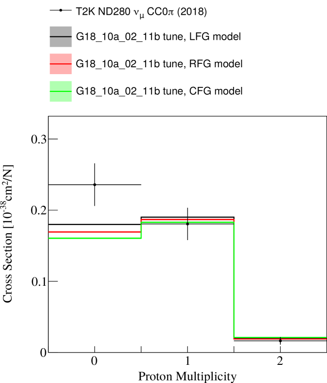
Figure 27: Comparison of G18_10a_02_11b against T2K ND280 $\nu_{\mu}$ CCNp0$\pi$ total cross section data as a function of the proton multiplicity [27]. Three calculations are shown for different nuclear models: LFG (black), RFG (red) and CFG (green).

VI.0.2 Nucleon Final State Interaction model variations

Mismodeling of nucleon FSI can cause migration between CC0p0$\pi$ and CCNp0$\pi$ samples [58]. Ref. [59] suggests increasing the nucleon mean-free path in cascade models might improve the agreement with CCNp0$\pi$ data from T2K ND280 and MINER$\nu$A. This possibility is explored here. The effect of the mean-free path implementation is validated against proton transparency data for carbon.

A crucial test for FSI models is to be able to reproduce nuclear transparency data from electron scattering experiments. Transparency is defined as the probability for the knocked-out nucleon to not undergo FSIs in the nuclear environment and it can be measured using electrons or neutrinos. In transparency measurements, the final-state nucleon is produced inside the nucleus. This feature is common with neutrino experiments, making transparency data extremely valuable to characterize and test FSI modeling uncertainties. Unfortunately, nuclear transparency measurements are scarce. Few data points on proton transparency on carbon as a function of the proton momentum are available in Ref. [60, 61, 62, 63].

Transparency can be easily calculated within MC event generators as a ratio between the distribution of final-state protons which did or did not rescatter while leaving the nuclear environment. Ref. [58] provided the first direct comparison of transparency calculations using a neutrino event generator. This analysis took into account the experimental acceptances of the electron scattering experiments in the transparency definition. Such an analysis could be replicated in GENIE; however, it is out of the scope of the present work. To be able to compare GENIE’s transparency calculations with data, we scale the GENIE predictions by the ratio between the transparency prediction from Ref. [58] with and without acceptance cuts. This approach was used in Ref. [50].

The effect on proton transparency calculations for carbon when varying the mean-free-path is shown in Fig. 29. The red and blue bands show the effect on the predictions when scaling up and down the nucleon mean-free path by 10% and 30% respectively. The 10% variation describes the data points with proton kinetic energies above 600 MeV within the 1$\sigma$ error bound. The 30% variation covers all the data available. Fig. 29 suggests that at most a 30% variation of the mean-free-path is feasible for low-momentum protons. This is also supported by Ref. [50], where the authors observed a strong model dependency at low proton kinetic energies. Another article [56] finds that low momentum protons have a small re-scattering probability [56], reinforcing the need of a more realistic model for the nuclear ground state.

The impact on the T2K ND280 cross section of variations in the nucleon mean-free path is shown in Fig. 28 as a function of proton multiplicity. It is observed that a higher nucleon mean-free path results in an increase of the proton multiplicity. A higher cross-section is predicted for events with no protons above detection threshold when reducing the mean-free path. However, variations of the mean-free path are not enough to explain the observed tension.

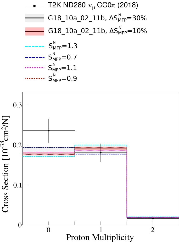
Figure 28: Comparison of the G18_10a_02_11b tune against T2K ND280 $\nu_{\mu}$ CCNp0$\pi$ total cross-section data as a function of the proton multiplicity. The GENIE prediction (black) is calculated using the G18_10a_02_11b. The error bands correspond to the expected uncertainty when varying the nucleon mean free path by 10% (red) and 30% (grey).

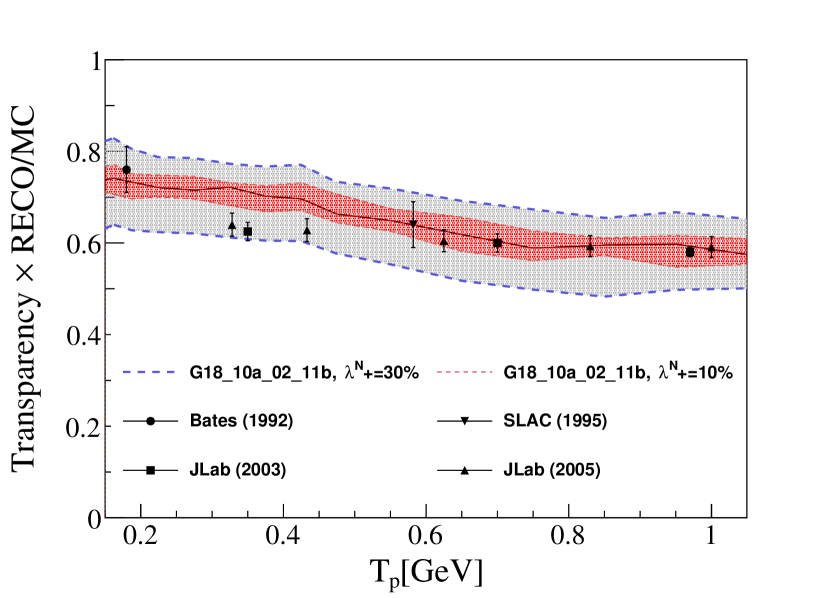
Figure 29: Comparison of proton transparency in carbon against the available electron scattering data [60, 61, 62, 63]. The GENIE prediction (black) is calculated using the G18_10a_02_11b. The error bands correspond to the expected uncertainty when varying the nucleon mean free path by 10% (red) and 30% (grey). The predictions have been corrected according to experiments acceptance effects as determined in Ref. [58].

Another possible line of study would be to determine whether more elaborate FSI models can resolve the tension. The hA and hN FSI models are build on a simplistic view of the nuclear environment. More complex approaches offer an improved description of CCNp0$\pi$ data [64, 65, 27]. Such a study is out of the scope of this paper.

VII Conclusions

This article describes the first neutrino-nucleus cross-section tuning effort within the GENIE Collaboration. The goal of this work is to tune GENIE against CC0$\pi$ data and quantify the major sources of CC0$\pi$ modelling uncertainties. In total, five partial tunes using double-differential flux-integrated $\nu_{\mu}$ or $\overline{\nu}_{\mu}$ CC0$\pi$ cross-section measurements on carbon as a function of the outgoing muon kinematics. Each tune is performed with data from either MiniBooNE, T2K ND280 or MINER$\nu$A following the same analysis procedure. Even though these experiments all use carbon as target, they are exposed to different neutrino beams, which peak at a different energy: the MiniBooNE and T2K fluxes peak below 1 GeV, whereas the MINER$\nu$A flux peaks at 3 GeV. Hence, this work exploits tuning to study possible energy dependencies of components of the CC0$\pi$ cross section by comparing each of the partial tune results. This analysis is based on the G18_10a_02_11b CMC, which was previously tuned against free nucleon data [5].

This tune confronted a number of new challenges with respect to previous GENIE free nucleon tuning efforts. This led to important changes in the GENIE tuning software. In particular, modern nuclear data provide the full correlation between the data release bins due to systematic uncertainties. In order to incorporate this information in the analysis, the definition of the $\chi^{2}$ is modified to avoid the Peele’s Pertinent Puzzle, which leads to nonphysical normalization factors.

This analysis considers a total of seven parameters which attempt to capture the basic features of the component interactions - QEL, 2p2h, and RES as implemented in the G18_10a_02_11b model set. Some of the parameters used in this work affect the simulation of neutrino interactions on free nucleon. We chose to constrain these parameters with correlated priors coming from previous GENIE tunes to bubble chamber data [5]. In addition, new parametrizations that encapsulate possible nuclear uncertainties were developed, using the Valencia model [13] for the QEL and 2p2h processes as a basis for choosing parameters. These affect the strength of the RPA correction for CCQEL calculations in a nuclear environment as well as the strength and shape of the 2p2h cross section – these are the main topic of this work. Other relevant CC0$\pi$ parameterizations that affect the nuclear or FSI models are discussed. These are found to be highly correlated with other aspects of the tune or not too sensitive to the CC0$\pi$ data considered in the tune. For these reasons, these are not included in the tunes presented here.

All tunes present a common trend: the QEL and 2p2h cross sections are enhanced and there is a preference for the QEL cross section with RPA corrections. In addition, the tune results are in agreement with the priors imposed on free nucleon parameters. Despite similarities, a clear energy dependence is observed for the 2p2h cross-section shape: the MiniBooNE and T2K tunes enhance the 2p2h cross section at the nucleon region, $W=M_{N}$, while suppressing it at the $\Delta$ region, $W=M_{\Delta}$. Alternatively, both MINER$\nu$A tunes enhance the cross section in both regions, with an even higher scaling factor at the $\Delta$ region. This suggests a dependence of the CC0$\pi$ cross section on the neutrino energy which is manifested in this work as a change in the shape and strength of the 2p2h cross section.

Tensions between the various CC0$\pi$ partial tunes and existing CCNp0$\pi$ data from T2K ND280, MINER$\nu$A and MicroBooNE exist. These results were shown in Table 6 and are a key result of this work. Parameters that give good agreement with one data set give poor $\chi^{2}$ values for the other data sets. Since MiniBooNE and T2K are at very similar energies, this indicates tensions between the data sets of the two experiments. In all cases, the tunes over-predict CCNp0$\pi$ data. This tension was further investigated with a dedicated tune, which is performed using MINER$\nu$A $\nu_{\mu}$ CCNp0$\pi$ data. The result suggests that a reduction of the QEL and 2p2h cross sections would improve the agreement with all CCNp0$\pi$ data, contradicting the CC0$\pi$ partial tunes. This tune also improves the agreement with MicroBooNE CCNp0$\pi$ data, suggesting that a possible $A$-dependence on the tune parameters is small, as was indicated in the MicroBooNE tune [10]. The disagreement with CCNp0$\pi$ data is further explored in this paper, highlighting the importance of using a more realistic nuclear model and possible changes to FSI models to describe existing CCNp0$\pi$ data. Tensions between neutrino and anti-neutrino tunes are also observed, suggesting the need of an additional modelling uncertainty. The observed tensions must be addressed before attempting to perform a global tune with all the available data.

VIII Acknowledgements

We would like to thank Andy Buckley (University of Glasgow, UK) and Holger Schultz (Institute of Particle Physics Phenomenology, University of Durham, UK) for their support interfacing the Professor tool with the software products that underpin the GENIE global analyses. We would like to thank the CC-IN2P3 Computing Center, as well as the Particle Physics Department at Rutherford Appleton Laboratory for providing computing resources and for their support. This work, as well as the ongoing development of several other GENIE physics tunes was enabled through a PhD studentship funded by STFC through LIV.DAT, the Liverpool Big Data Science Centre for Doctoral Training (project reference: 2021488). The initial conceptual and prototyping work for the development of the GENIE / Professor interfaces, as well as for the development of the GENIE global analyses framework that, currently, underpins several analyses, was supported in part through an Associateship Award by the Institute of Particle Physics Phenomenology, University of Durham. We thank: Stephen Dolan and Jaafar Chakrani for providing the method to correct for Peelle’s Persistent Paradox; Daniel Ruterbories and Stephen Dolan for guidance to implement MINER$\nu$A’s and T2K’s analysis requirements in GENIE Comparisons; Xianguo Lu for discussion and comments on the paper.

Appendix A Kinematic quantities of interest for CC0$\pi$ measurements

Differential neutrino cross-section measurements are given as a function of different kinematic quantities. In this paper, these kinematic quantities are classified into direct, inferred with an underlying process hypothesis or inferred without an underlying process hypothesis.

A.1 Direct

Kinematic quantities that can be measured by the detector are classified as direct. For instance, an example of direct quantity would be the muon momentum, $p_{\mu}$, or angle with respect to the beam-line axis, $\theta_{\mu}$. In some cases, the muon kinetic energy, $T_{\mu}$, is used instead. All cross-section measurements specified in Tab. 2 released data as a function of the muon kinematics. Depending on the detector capabilities, direct quantities can also be related to proton kinematics. We refer to proton momentum and angle as $p_{p}$ and $\theta_{p}$ respectively.

Muon direct quantities depend strongly on the neutrino energy and these are less sensitive to nuclear effects. This motivated the recent efforts on the study of more exclusive topologies that allow measurement of the cross section as a function of the outgoing-proton kinematics [27, 29, 32, 31]. These depend weekly on the neutrino energy and are significantly altered by nuclear effects [40].

In some cases, the differential cross-section measurements are presented as a function of the reconstructed direct quantities. Kinematic quantities in the reconstructed space are denoted with a ’reco’ superscript. For instance, $p_{\mu}^{\text{reco}}$ stands for reconstructed muon momentum.

A.2 Inferred kinematic with an underlying process hypothesis

This category includes measurements that rely on the reconstruction of neutrino properties assuming a specific interaction type. For instance, the kinematics of a CC0$\pi$ event can be reconstructed under the hypothesis that the initial nucleon was at rest and that there is no inelastic production of mesons in the final state (QEL hypothesis). Under this hypothesis, the reconstructed neutrino energy ($E_{\nu}^{\text{QEL}}$) and squared four-momentum transferred ($Q_{\text{QEL}}^{2}$) are:

$$E_{\nu}^{\text{QEL}}=\frac{M_{f}^{2}-(M_{i}-E_{b})^{2}-M^{2}_{\mu}+2(M_{i}-E_{b})E_{\mu}}{2(M_{i}-E_{b}-E_{\mu}+p_{\mu}\cos\theta_{\mu})}$$ (2)

$$Q^{2}_{\text{QEL}}=2E_{\nu,\text{QEL}}(E_{\mu}-p_{\mu}\cos\theta_{\mu})-M^{2}_{\mu}$$ (3)

where $M_{i}$ ($M_{f}$) is the initial (final) nucleon mass, $M_{\mu}$ is the muon mass, and $E_{\mu}$ is the muon energy. For the neutrino analysis, $M_{i}=M_{n}$ and $M_{f}=M_{p}$, whereas $M_{i}=M_{p}$ and $M_{f}=M_{n}$ for the antineutrino case. The binding energy, $E_{b}$, depends on the target type. Its specific value is provided in each analysis.

The main disadvantage of using these quantities is that the underlying hypothesis is uncertain. The presence of the nuclear environment complicates the characterization of event topologies: no single-event topology is produced only by a single underlying process. This is highlighted by the T2K ND280 results on inferred kinematics [27]. In their analysis, they reconstruct the energy and momentum of the outgoing proton assuming a QEL interaction. Instead of presenting the cross-section measurement as a function of the inferred with kinematic with an underlying process quantities, they used the difference between the direct and the inferred one. In particular, T2K ND280 explored this quantity for the proton kinematics:

$$\begin{gathered}\Delta p_{p}\equiv\left|\mathbf{p}_{p}^{\text{direct}}\right|-\left|\mathbf{p}_{p}^{\text{QEL}}\right|,\\ \Delta\theta_{p}\equiv\left|\theta_{p}^{\text{direct}}\right|-\left|\theta_{p}^{\text{QEL}}\right|,\\ |\Delta\mathbf{p}_{p}|\equiv\left|\mathbf{p}_{p}^{\text{direct}}-\mathbf{p}_{p}^{\text{QEL}}\right|.\end{gathered}$$ (4)

These are referred to as proton inferred kinematics quantities. Here, the superscript indicates whether the kinematic quantity is direct (i.e $\mathbf{p}_{p}^{\text{direct}}$) or inferred (i.e. $\mathbf{p}_{p}^{\text{QEL}}$) . The reconstructed proton energy and momentum under the QEL hypothesis are:

$$E_{p}^{\text{QEL}}=E_{\nu}^{\text{QEL}}-E_{\mu}+M_{p}$$

$$\mathbf{p}_{p}^{\text{QEL}}=\left(-p_{\mu}^{x},-p_{\mu}^{y},-p_{\mu}^{z}+E_{\nu}^{\text{QEL}}\right)$$

These kinematic quantities can be used to highlight nuclear effects in CC0$\pi$ measurements, as the quantities defined in Eq. 4 deviate from zero when nuclear effects are present.

A.3 Inferred without an underlying process hypothesis

This category includes those kinematical quantities which are inferred from direct ones but do not assume a specific underlying interaction process. An example of interest for this work is the Single-Transverse Kinematic Imbalance (STKI) variables [40]. STKI provide direct constraints on nuclear effects that, in some cases, have a weak dependence on the neutrino energy. STKI quantities are inferred from the muon and primary state hadron kinematics and only detectors capable of measuring low energy hadrons can provide such information. So far, only T2K ND280 and MINER$\nu$A have released single-differential flux-integrated cross-section measurements as a function of these quantities [27, 29, 30].

The transverse momentum imbalance, $\delta\mathbf{p}_{T}$, is defined as the sum of the transverse muon and proton momentum:

$$\delta\mathbf{p}_{T}\equiv\mathbf{p}^{\mu}_{T}+\mathbf{p}^{p}_{T}.$$

As the neutrino travels in the longitudinal direction, the transverse muon momentum is related to the transverse momentum transfer as $\mathbf{p}^{\mu}_{T}=-\mathbf{q}_{T}$. The angle between $\delta\mathbf{p}_{T}$ and $-\mathbf{p}^{\mu}_{T}$ is known as boosting angle, $\delta\alpha_{T}$:

$$\delta\alpha_{T}\equiv\arccos\left(\frac{-\mathbf{p}_{T}^{\mu}\cdot\delta\mathbf{p}_{T}}{p_{T}^{\mu}\delta p_{T}}\right).$$

The deflection of the nucleon with respect to $\mathbf{q}_{T}$ is measured with the $\delta\phi_{T}$ angle:

$$\delta\phi_{T}\equiv\arccos\left(\frac{-\mathbf{p}_{T}^{\mu}\cdot\mathbf{p}_{T}^{p}}{p_{T}^{\mu}p_{T}^{p}}\right).$$

A more recent study investigates the CC0$\pi$ cross-section dependency on the muon-proton momentum imbalances parallel ($\delta p_{Ty}$) and longitudinal ($\delta p_{Tx}$) to the momentum transfer in the transverse plane [30]. These quantities are mathematically defined as:

$$\delta p_{Tx}= \ \left(\hat{\mathbf{p}}_{\nu}\times\hat{\mathbf{p}}_{T}^{\mu}\right)\cdot\delta\mathbf{p}_{T}$$

$$\delta p_{Ty}= \ -\hat{\mathbf{p}}^{\mu}_{T}\cdot\delta\mathbf{p}_{T}$$

given the Cartesian coordinate system defined with respect to the neutrino and muon kinematics. The neutrino direction is given by $\hat{\mathbf{p}}_{\nu}$. All these quantities define what experiments refer to as STKI variables.

A graphical representation of the definition of the STKI variables for a neutrino interaction with and without nuclear effects is shown in Fig. 31. When the interaction occurs with a static free nucleon, i.e. no nuclear effects, ${\mathbf{p}^{\mu}_{T}=-\mathbf{p}^{p}_{T}}$, $\delta\mathbf{p}_{T}=0$ and $\delta\phi_{T}=0$, see Fig. 30(a). However, this picture is modified by Fermi motion, nucleon correlations, non-QEL interactions and FSI. If FSI effects and nucleon correlations are neglected, $\delta\mathbf{p}$ coincides with the initial nucleon momentum $\mathbf{p}_{N_{i}}$. Moreover, $\delta\alpha_{T}$ is uniform due to the isotropic nature of the Fermi motion. FSI effects smear the $\delta\mathbf{p}_{T}$ distribution and modify the shape of the $\delta\alpha_{T}$ distribution. In GENIE, the hA FSI model enhances the cross section at $\delta p_{T}>0.2$ GeV/c and $\delta\alpha_{T}\sim 180^{\circ}$; see Fig. 31. This region is refereed to as high-transverse kinematic imbalance region.

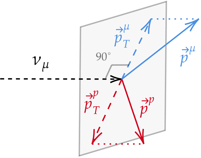
(a)

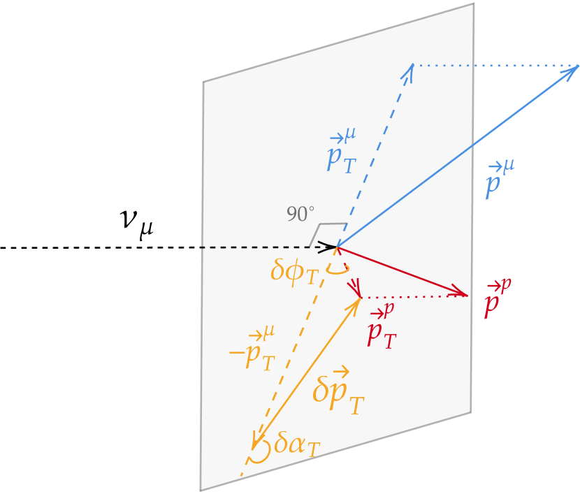
(b)

Figure 30: Graphical definition of the STKI variables in a $\nu_{\mu}$ CCQEL neutrino interaction on a nuclear target. The incoming neutrino, represented as a dashed arrow, interacts with a free nucleon at rest (a) or with a bound nucleon subject to Fermi motion (b). The outgoing muon (proton) is represented in blue (red). The transverse plane is represented in grey. The incoming neutrino is perpendicular to the transverse plane. Nuclear effects distortion the free-nucleon picture (a) creating an imbalance between the muon and nucleon transverse momentum (b). The STKI variables that define this imbalance are highlighted in orange.

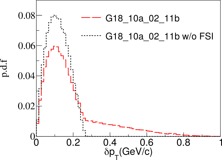
(a)

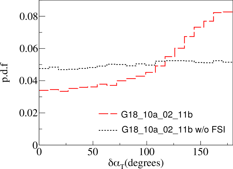
(b)

Figure 31: Probability density function of $\delta p_{T}$ and $\delta\alpha_{T}$ for the G18_10a_02_11b tune with (a) and without (b) FSI. Both predictions are obtained simulating $\nu_{\mu}$ CCQEL interactions only on ¹²C at 1 GeV with the G18_10a_02_11b tune.

Ref. [40] demonstrated that the $\delta p_{T}$ and $\delta\alpha_{T}$ dependence on the neutrino energy is smaller than possible uncertainties due to FSI modeling. The $\delta\phi_{T}$ variable has a stronger dependence on the neutrino energy as it scales with $\delta p_{T}/p^{\mu}_{T}$: at higher neutrino energies, the distribution at small angles becomes narrower. The dependency of the STKI variables in GENIE with the neutrino energy is shown in Fig. 32. Changes in the neutrino energy affect mostly the tail of the $\delta p_{T}$ distribution and the $\delta\alpha_{T}$ distribution at backward angles.

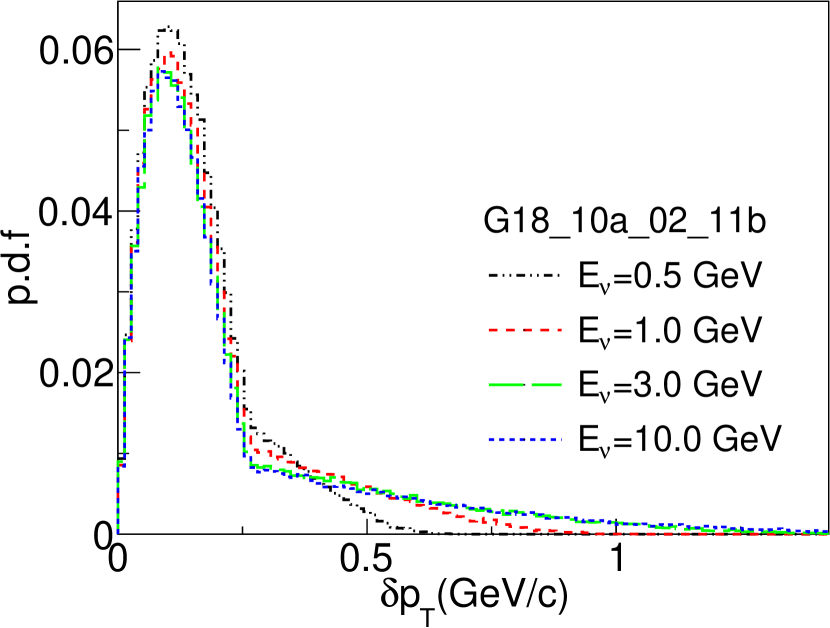
(a)

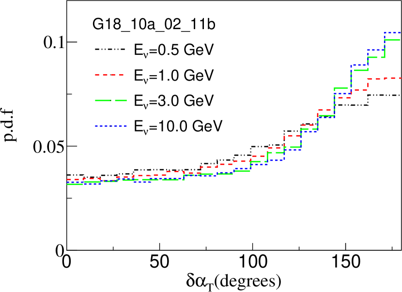
(b)

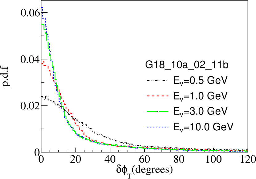
(c)

Figure 32: Probability density function of STKI variables. The predictions are obtained simulating $\nu_{\mu}$ CCQEL interactions only on ¹²C with the G18_10a_02_11b tune at different neutrino energies.

Appendix B Comparisons G18_10_02_11b against neutrino-nucleus CC0$\pi$ data

This section offers with comparisons of GENIE against all CC0$\pi$ and CCNp0$\pi$ data available from MiniBooNE, T2K, MINER$\nu$A and MicroBooNE. The corresponding GENIE predictions are obtained by replicating the analysis within GENIE: neutrino interaction events are simulated for each experiment given the neutrino flux, target material, and analysis cuts. The normalized neutrino flux spectra is reported in Fig. 1. With this information, the GENIE prediction for the corresponding differential flux-integrated cross section is evaluated.

The format of all the comparisons with data reported in this appendix is common: the data and differential cross-section prediction are represented in black. In addition, the contribution from different interaction models is shown for CCRES, CC2p2h and CCDIS/SIS. The contribution to the G18_10a_02_11b predictions from CCDIS/SIS events is really small at the neutrino energies considered in this work. For this reason, the contribution is grouped into a single category (DIS). The 2p2h contribution is divided further into four categories that depend on the event invariant mass, $W$. The $W$ regions are:

• $W<M_{N}=938$ MeV/c²

• $M_{N}<W<W_{\text{Dip}}=1120$ MeV/c²

• $W_{\text{Dip}}<W<M_{\Delta}=1232$ MeV/c²

• $W>M_{\Delta}$

The data error bars include statistical and systematic uncertainties. The errors on the $x$-axis represent the bin width used in the original analysis.

B.1 MiniBooNE CC0$\pi$ cross-section measurement

The MiniBooNE experiment studies neutrinos produced with the BNB [7]. MiniBooNE published the first-high statistics $\nu_{\mu}$ and $\overline{\nu}_{\mu}$ CC0$\pi$ flux-integrated double differential cross-section measurement on carbon, at $\langle E_{\nu}\rangle\sim 800$ MeV and $\langle E_{\overline{\nu}}\rangle\sim 500~{}\text{MeV}$ respectively [25, 26]. The flux-unfolded total cross section, $\sigma\left(E_{\nu}^{\text{QEL}}\right)$, and the flux-integrated single differential cross section as a function of the squared four-momentum transferred, $d\sigma/dQ^{2}_{\text{QEL}}$, were also reported.

Both MiniBooNE analyses study CC0$\pi$ events with a muon in the final state and no pions. The signal topology of a muon in the detector is described in two sub-events: the first one associated with the primary Cherenkov light from the muon, and the second one, produced by the Cherenkov light from the Michel electron, which is produced in the muon decay. This requirement provides a sample of mostly CC events, as neutral-current events only have one sub-event.

Positively charged pions produced in the detector leave a distinct signature in the detector, as the $\pi^{+}$ decays immediately into a muon and a muon neutrino. The Cherenkov light from the $\pi^{+}$ contributes to the total light of the primary muon. This process can be distinguished from a CCQEL interaction as the muon produced from the pion decay will also decay into a Michel electron (three sub-events). Negatively charged pions are absorbed by the nuclear environment and contribute to the CC0$\pi$ topology. In the GENIE predictions, pion production events are removed by requiring no pions in the final state.

Recoil protons also emit scintillation light. However, such scintillation light signal produced is either indistinguishable from the muon signal or its momentum below the Cherenkov threshold. For this reason, no requirements based on the recoil proton are considered in the MiniBooNE analyses.

The analysis considers further model-dependent cuts to correct for backgrounds and extract the CCQEL cross-section from the CC0$\pi$ sample. In the original publication, these are referred to as irreducible backgrounds. An example of irreducible background is CC1$\pi$ events that were not removed by the cut on the pion subevent topology or pion production events in which the pion is absorbed. This is corrected using a MC simulation tuned to $\nu_{\mu}$ CC1$\pi$ MiniBooNE data. Information on $\nu_{\mu}$ CC1$\pi^{+}$ sample is used to characterize this background and correct for single-pion events which were not removed by the CC0$\pi$ selection criteria in the neutrino and antineutrino analyses. This procedure is one of the main limitations of this dataset as it incorporates strong biases in the reported measurement. The contribution to the cross-section measurement from irreducible backgrounds is also reported, allowing the comparison against CC0$\pi$ data.

The quality of the MiniBooNE CC0$\pi$ data release is poor in comparison with the rest. The MiniBooNE collaboration provided measurements in bins of $T_{\mu}$ and $\cos\theta_{\mu}$, but did not provide the bin-to-bin covariances for either of the two measurements. Instead, they quoted a normalization systematic uncertainty of $\sim 10.7$% ($17.2$%) for the neutrino (antineutrino) measurement. As suggested by Ref. [25], this error is added as a systematic in our database, effectively including a correlation between the bins.

In Figs. 2 and 33, the flux-integrated double differential $\nu_{\mu}$ and $\overline{\nu}_{\mu}$ CC0$\pi$ cross section data as a function of $p_{\mu}$ and $T_{\mu}$ are compared against GENIE. The main observation is that the GENIE tune under-predicts the data. In particular, the G18_10a_02_11b disagreement with the data are more significant at backward angles, where the cross-section is determined by CCQEL events only. The disagreement is also observed at forward angles, where there is a significant contribution from non-QEL events.

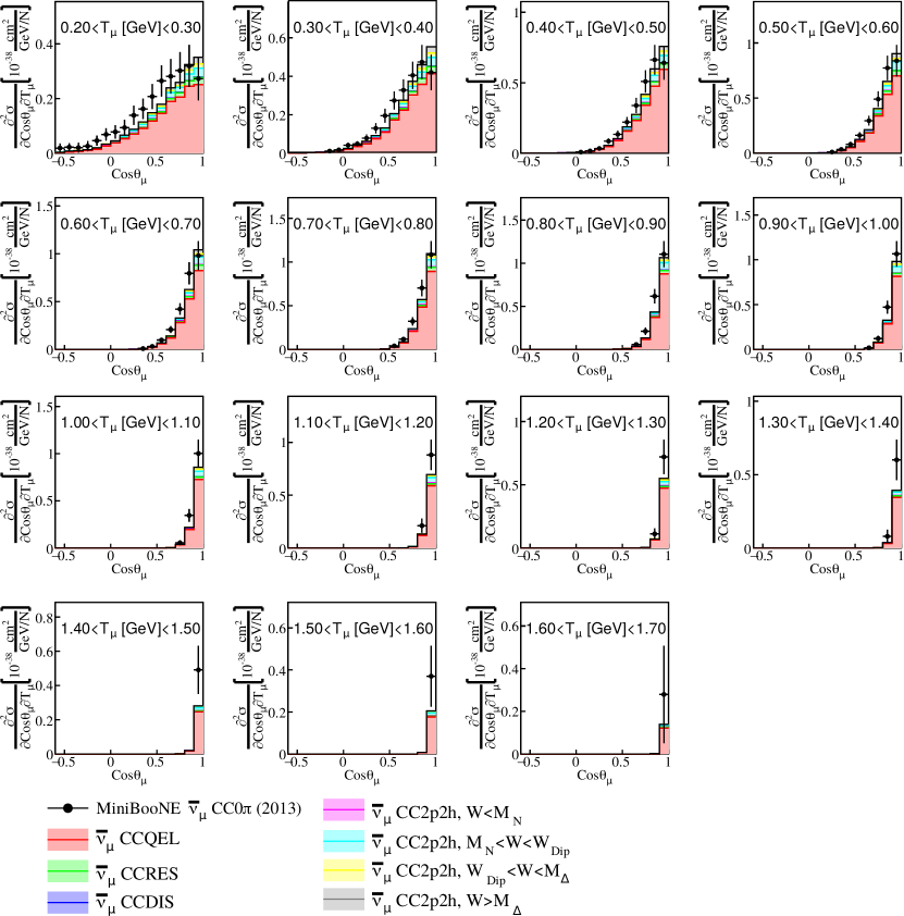
Figure 33: MiniBooNE $\overline{\nu}_{\mu}$ CC0$\pi$ double differential flux-averaged cross section as a function of the muon angle, $\theta_{\mu}$, and kinetic energy, $T_{\mu}$ [26]. The corresponding slices on $T_{\mu}$ are compared against the G18_10a_02_11b tune. The GENIE prediction is divided into different categories: CCQEL, CCRES, CC2p2h and CCDIS.

B.2 T2K CC0$\pi$ cross-section measurements

The Tokai-to-Kamioka (T2K) experiment is an accelerator-based long-baseline experiment that studies neutrino oscillations. Neutrinos are generated at the Japan Proton Accelerator Research Complex (J-PARC) facility [6]. The target for the neutrino beam is 280 m away from the T2K near detectors [2]: INGRID, WAGASCI and ND280. The T2K ND280 detector is used to measure neutrino interactions on carbon at $\langle E_{\nu}\rangle\sim 600$ MeV. The WAGASCI module was recently added to the T2K ND facility and it measures neutrino interactions at 0.86 GeV. Details on the detector setup can be found in Ref. [27, 37]. Most measurements described here use the detector central tracker region, composed of three time projection chambers (TPC) and two fine-grained detectors (FGD1 and FDG2). The FGDs are the target mass and are also used to track charged particles. Carbon measurements use the FGD1 as the target mass. The central region is surrounded by an electromagnetic calorimeter (ECal), which is contained within a magnet. This setup allows measuring the particle charge and momentum. This information, together with energy deposition, is used to identify charged particles.

The first double-differential $\nu_{\mu}$ CC0$\pi$ measurement provided by T2K ND280 was released back in 2015 [41]. This measurement is surpassed by Ref. [27], which considers improved constraints on systematic uncertainties. Ref. [27] provides additional measurements including double- and triple-differential measurements for different proton multiplicities as well as two CCNp0$\pi$ single-differential cross-section measurements as a function of STKI and proton inferred kinematics quantities.

All measurements from Ref. [41] require one muon and no pions in the final state, regardless of the number of nucleons in the event. Any event must contain at least one track in the TPC, which must be either a muon or a proton. If it is a proton, they look for a muon-like track in the FDG1 or ECal. Other events with tracks that are not consistent with the muon-like or proton-like signature are rejected. Events with low-momentum charged or neutral pions are removed by requiring no Michel electrons or photons. At the MC level, this is implemented by removing events with pions or photons in the final state, respectively.

The selected sample is divided further depending on the number of protons above the detection threshold of 500 MeV/c: no protons (CC0p0$\pi$), one proton (CC1p0$\pi$) or more than one visible proton (CC2p0$\pi$) in the final state. The CC0p0$\pi$ and CC1p0$\pi$ are double- and triple-differential cross-section measurements as a function of the muon and muon and proton kinematics respectively. The total CC2p0$\pi$ cross-section is also reported. The STKI and proton inferred kinematics are obtained with the CCNp0$\pi$ sample: they require the presence of at least one visible proton ($p_{p}>500$ MeV/c).

T2K ND280 Analysis	$p_{p}$	$\cos\theta_{p}$	$p_{\mu}$	$\cos\theta_{\mu}$
CC0p0$\pi$	$<500$ MeV/c (or no proton)
CC1p0$\pi$	$>500$ MeV/c
CCNp0$\pi$, STKI	$450<p_{p}<1000$ MeV/c	$>0.4$	$>250$ MeV/c	$>-0.6$
CCNp0$\pi$, proton inferred kinematics	$>450$ MeV/c	$>0.4$

Table 9: Phase-space restrictions for the T2K ND280 analyses from Ref. [27]. The proton cuts are only applied to the highest energy proton.

Efficiency corrections for $\nu_{\mu}$ CCNp0$\pi$ events can be model dependent. To avoid this, different kinematical restrictions are considered for each analysis, selecting regions in which the efficiency is flat or well understood. These are specified in Tab. 9. Events with more than one proton are reconstructed using the information from the highest energy one, which has to satisfy the kinematical limits of Tab. 9. The samples are not corrected for events with protons below the detection threshold or any of the kinematical cuts considered in the analysis. The same cuts are applied at the generator level when evaluating the GENIE predictions.

The GENIE comparison against the $\nu_{\mu}$ CC0p0$\pi$ double-differential cross section are presented in Fig. 34. The main contribution to the CC0p0$\pi$ topology comes from CCQEL events. The second contribution is from CC2p2h events with $M_{N}<W<W_{\text{Dip}}$. The contribution from 2p2h events with $W<M_{N}$ or $W>W_{\text{Dip}}$ is negligible for the CC0p0$\pi$ measurement. GENIE is under-predicting the data at backward angles.

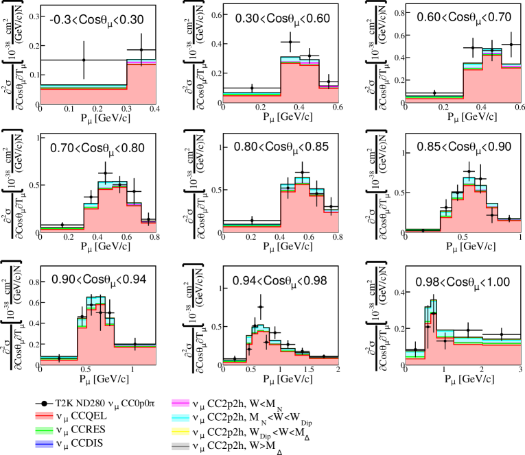
Figure 34: T2K ND280 flux-averaged $\nu_{\mu}$ CC0p0$\pi$ differential cross section as a function of the proton multiplicity [41]. The data are compared against the G18_10a_02_11b tune. The GENIE prediction is divided into different categories: CCQEL, CCRES, CC2p2h and CCDIS. For readability, the CC0p$0\pi$ high energy bins are not included in these plots.

This disagreement in the overall normalization is also observed in Fig. 5, which compares GENIE against the cross-section as a function of the proton multiplicity. This observation conflicts with $\nu_{\mu}$ CC1p0$\pi$ data, which is not under-predicted. There are some outstanding differences between the GENIE predictions for CC0p0$\pi$ and CC1p0$\pi$ data. Whilst the total contribution from 2p2h events is similar, the main 2p2h contribution comes from 2p2h events with $W>W_{\text{Dip}}$. In addition, the fraction from RES events is higher with respect to the CC0p0$\pi$ one.

Fig. 35 provides comparisons against $\nu_{\mu}$ CCNp0$\pi$ data as a function of the STKI variables, concluding that non-QEL interactions are essential to describe this data within regions of high transverse kinematic imbalance.

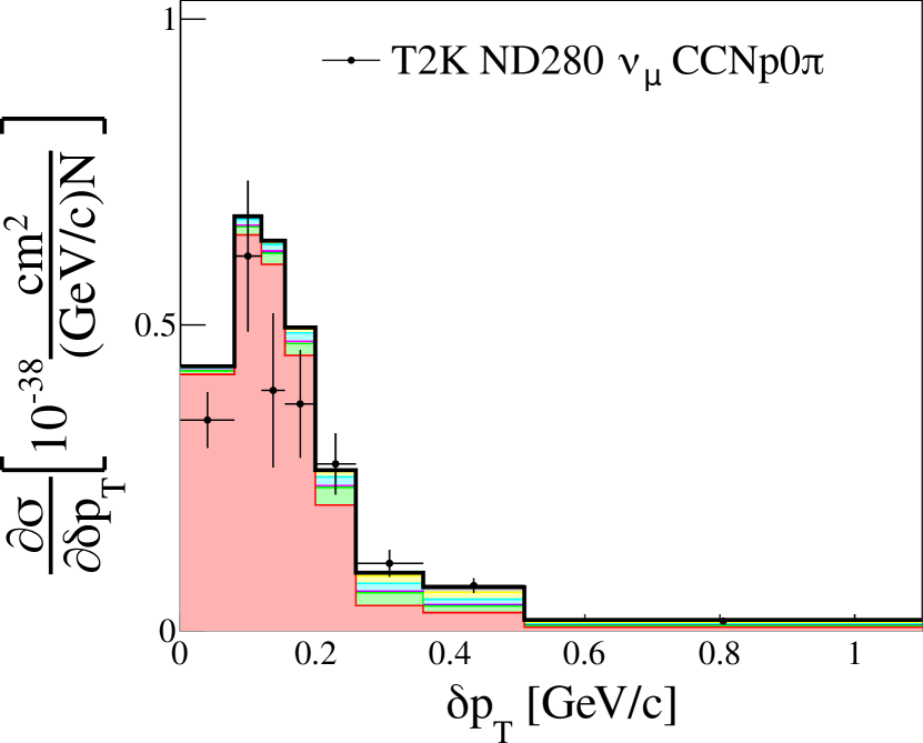
(a)

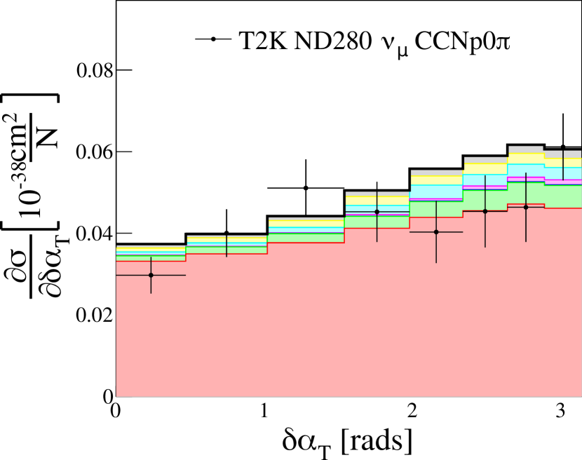
(b)

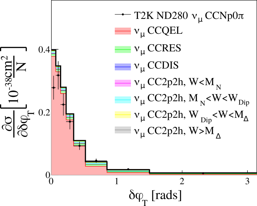
(c)

Figure 35: T2K ND280 flux-averaged $\nu_{\mu}$ CCNp0$\pi$ differential cross section as a function of STKI variables [41]. The data are compared against the G18_10a_02_11b tune. The GENIE prediction is divided into different interaction categories: CCQEL, CCRES, CC2p2h and CCDIS.

Antineutrino CC0$\pi$ cross section measurements are also available: $\overline{\nu}_{\mu}$ and $\overline{\nu}_{\mu}$+$\nu_{\mu}$CC0$\pi$ on water [35] and hydrocarbon at T2K ND280 [36], and $\overline{\nu}_{\mu}$ and $\overline{\nu}_{\mu}$+$\nu_{\mu}$CC0p0$\pi$ at the T2K WAGASCI, INGRID and Proton Module detectors [37]. Ref. [37] reports the $\overline{\nu}_{\mu}$ and the $\overline{\nu}_{\mu}+\nu_{\mu}$ CC0p0$\pi$ cross sections on water and hydrocarbon. For all measurements, the muon phase space is restricted to $p_{\mu}>400$ MeV/c and $\theta_{\mu}<30^{\circ}$. The analysis requires events with a muon and no visible pions ($p_{\pi}>200$ MeV/c, $\theta_{\pi}<70^{\circ}$) or protons ($p_{p}>600$ MeV/c, $\theta_{p}<70^{\circ}$). Fig. 36 shows the agreement of the G18_10a_02_11b tune for the T2K WAGASCI $\overline{\nu}_{\mu}$ CC0p0$\pi$ data. The GENIE prediction underpredicts the data as well when considering a higher neutrino flux ($\langle E_{\nu}\rangle=0.86$ GeV). At higher energies, the 2p2h contribution $W>W_{dip}$ is non-negligible.

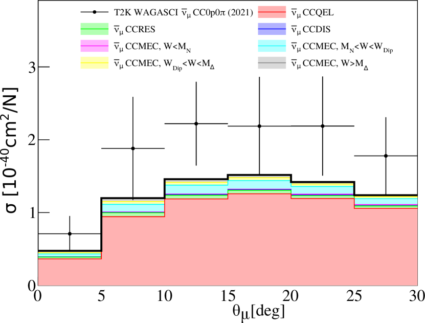
Figure 36: T2K WAGASCI flux-averaged $\overline{\nu}_{\mu}$ CC0p0$\pi$ differential cross section as a function of the muon angle. The data are compared against the G18_10a_02_11b tune. The GENIE prediction is divided into different interaction categories: CCQEL, CCRES, CC2p2h and CCDIS.

B.3 MINER$\nu$A CC0$\pi$ cross-section measurements

MINER$\nu$A studies neutrino interactions on nuclear targets for neutrino and antineutrino interactions at $\sim 1-10$ GeV at Fermilab [66, 67]. MINER$\nu$A’s detector is composed of a segmented scintillator detector surrounded by electromagnetic and hadronic calorimeters. The detector is situated 2.1 m upstream of the MINOS near detector [68], which is a magnetized iron spectrometer. MINOS is used to reconstruct the muon momentum and charge.

Neutrinos are generated at the NuMI beamline [8]. This beam has two configurations: low energy flux ($\langle E_{\nu}\rangle\sim 3.5$ GeV) and medium energy flux ($\langle E_{\nu}\rangle\sim 6$ GeV). The NuMI beam can operate in neutrino mode (FHC) and antineutrino mode (RHC). The FHC and RHC low energy flux predictions are shown in Fig. 1.

MINER$\nu$A extracted several CC$0\pi$ and CCNp$0\pi$ measurements using the NuMI low-energy flux [28, 38, 29, 30]. A CC0$\pi$ measurement using the NuMI medium energy flux is also available [33]. This review focuses on the CC0$\pi$ and CCNp0$\pi$ measurements obtained with the low-energy flux.

The exact target mixture is composed of carbon (88.51%), hydrogen (8.18%), oxygen (2.5%), titanium (0.47%), chlorine (0.2%), aluminium (0.07%), and silicon (0.07%). In the calculation of the GENIE predictions, only the three most abundant targets are considered. The relative mass abundances are renormalized to take this approximation into account. This simplifies the computing power and has a negligible effect on our predictions.

B.3.1 MINER$\nu$A $\nu_{\mu}$ and $\overline{\nu}_{\mu}$ CC0$\pi$ cross-section measurement

MINER$\nu$A reported the CC0$\pi$ differential flux-integrated cross-section as a function of muon momentum in the transverse ($T$) and longitudinal ($\parallel$) direction relative to the neutrino beam [28, 38]. The differential cross-section as a function of $E_{\nu}^{\text{QEL}}$ and $Q^{2}_{\text{QEL}}$ are reported as well [28]. The neutrino energy and the momentum transferred are reconstructed under the QEL hypothesis, described in Sec. A.2. The binding energy used to reconstruct $E_{\nu}^{\text{QEL}}$ according to Eq. 2 in their neutrino and antineutrino analysis is $E_{b}=34$ MeV and $E_{b}=30$ MeV respectively.

The $\nu_{\mu}$ CC0$\pi$ topology is defined as an event with one muon, $\mu^{-}$, any number of protons and neutrons, any photons below nuclear de-excitation energies, $E_{\gamma}\leq 10$ MeV, no mesons and no heavy or excited baryons in the final state. The MINER$\nu$A detector is not able to measure the muon charge as it does not have a magnetic field. For this reason, muons are identified by looking for tracks that have a match with the MINOS detector, which is used to determine the muon momentum and charge. Because of geometric acceptance, both analyses require $\theta_{\mu}<20^{\circ}$. Events containing low-energy photons are accepted as they can arise from nuclear de-excitation. Pions are removed by applying a cut on the recoil energy, $E_{\text{recoil}}\leq 500$ MeV, defined as the activity that is not coming from a muon or any tracked protons. $E_{\text{recoil}}$ is corrected for the calorimetric detector response [38]. The recoil energy does not include energy deposited at less than 150 mm from the neutrino vertex as it could be due to proton absorption nearby the vertex. Moreover, events with Michel electrons are removed, as they assume they come from a $\pi$ decay chain ($\pi\rightarrow\mu\rightarrow e$).

The $\overline{\nu}_{\mu}$ CC0p0$\pi$ topology [38] is similar to the $\nu_{\mu}$CC0$\pi$ one, with some differences. Due to the nature of this interaction, the muon must be positively charged. Moreover, the analysis requires there are no visible protons in the final state, i.e. protons with kinetic energy above 120 MeV. Finally, mesons are removed using the information on the recoil energy deposited outside the vertex region only.

The GENIE prediction is evaluated with MC events that satisfy the criteria specified above with few exceptions: the removal of events with mesons in the final state is based on true information only. Baryons, are short living and decayed into mesons using the GENIE particle decayer. The requirements on the removal energy are not implemented in our MC analysis either as the data was already corrected for this effect.

GENIE comparisons against the double-differential $\nu_{\mu}$ CC$0\pi$ measurement is shown in Figs. 3 and 38 for $\overline{\nu}_{\mu}$ CC0p$0\pi$ data. For both $\nu_{\mu}$ and $\overline{\nu}_{\mu}$ data, the G18_10a_02_11b underestimates the data. This is true especially in the phase-space regions in which 2p2h events dominate. In high $p_{T}$ regions, where the contribution of 2p2h events is negligible, the agreement improves. This can be seen for the $0.85<p_{T}<2.5$ GeV/c slices in Fig. 3. Consequently, the reconstructed neutrino energy is also under-predicted, as observed in Fig. 37.

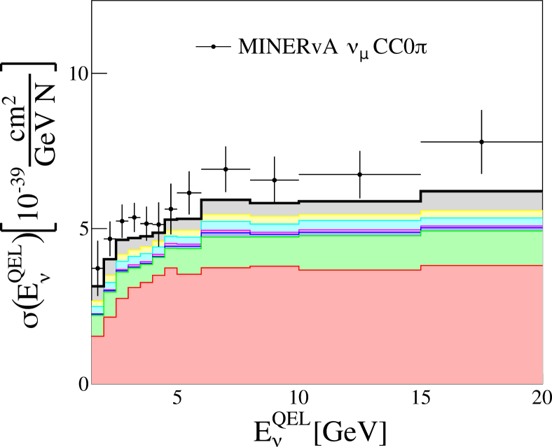
Figure 37: MINER$\nu$A $\nu_{\mu}$ CC0$\pi$ flux-averaged cross-section as a function of the reconstructed neutrino energy, $E_{\nu}^{\text{QEL}}$ [28]. The data are compared against the G18_10a_02_11b tune. The notation for the histogram is the same as in Fig. 35.

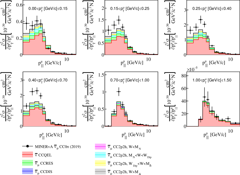
Figure 38: MINER$\nu$A $\overline{\nu}_{\mu}$ CC0$\pi$ double differential flux-averaged cross-section as a function of the muon longitudinal momentum, $p_{\parallel}$, and transverse momentum, $p_{T}$ [28]. The corresponding slices on $p_{T}$ are compared against the G18_10a_02_11b tune. The GENIE prediction is divided into different interaction categories.

B.3.2 MINER$\nu$A $\nu_{\mu}$ CCNp0$\pi$ production cross-section measurement

The MINER$\nu$A Collaboration released two CCNp0$\pi$ analyses: single-differential cross-section measurements as a function of $\delta p_{T}$, $\delta p$, $\delta\alpha_{T}$ and $\delta\phi_{T}$ [29], and a single-differential measurement as a function of $\delta p_{Ty}$ or $\delta p_{Tx}$, respectively [30].

In both analyses, the topology is defined as events with a muon, no mesons and at least one proton in the final state that satisfy the following conditions:

$$1.5~{}\text{GeV}/c<p_{\mu}<10~{}\text{GeV}/c\enskip\text{and}\enskip\theta_{\mu}<20^{\circ},$$

$$0.45~{}\text{GeV}/c<p_{p}<1.2~{}\text{GeV}/c\enskip\text{and}\enskip\theta_{p}<70^{\circ},$$

where $p_{\mu}$ ($p_{p}$) and $\theta_{\mu}$ ($\theta_{p}$) are the muon (lead proton) momentum and opening angle with respect to the neutrino direction. The lead proton is defined as the proton with the highest energy that satisfies the phase space cuts mentioned above.

In this case, the G18_10a_02_11b tune is not under-predicting the data, see Fig. 4 and Fig. 39. This fact, already observed in T2K data, reflects a possible tension between CC$0\pi$ and CCNp$0\pi$ measurements. The breakdown into different interaction modes highlights the 2p2h model dependence with $W$ at different proton momenta: 2p2h events with low (high) $W$ dominate at low (high) proton momentum. The contribution from RES events is most significant for low proton momenta, small proton angles and $\delta\alpha_{T}\sim 180^{\circ}$. In fact, non-QEL events dominate in regions of high transverse kinematic imbalance, such as $\delta p_{T}>0.2$ GeV/c.

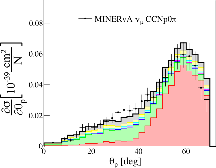
(a)

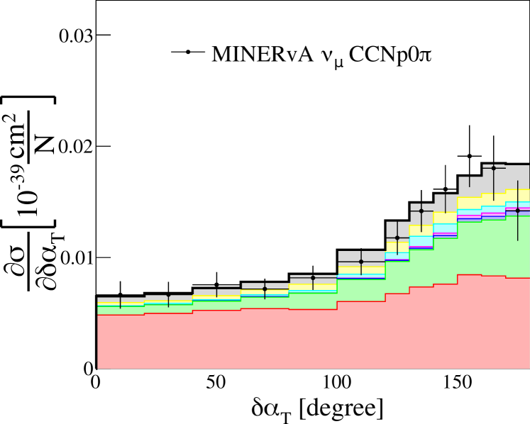
(b)

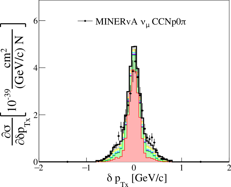
(c)

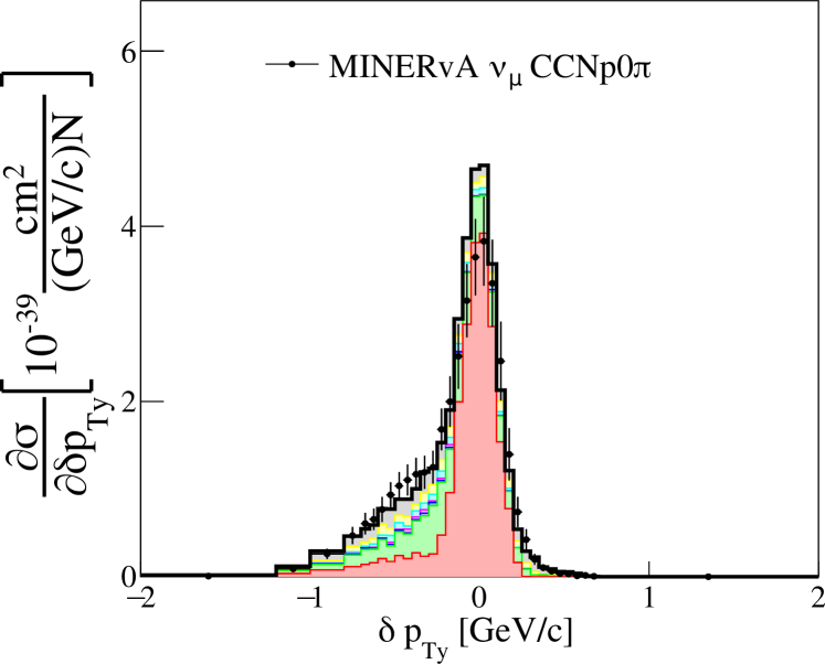
(d)

Figure 39: MINER$\nu$A $\nu_{\mu}$ CCNp0$\pi$ differential flux-averaged cross-section as a function of STKI variables [29, 30]. The data are compared against the G18_10a_02_11b tune. The GENIE prediction is divided into interaction modes. The notation for histograms is the same as in Fig. 35.

B.4 MicroBooNE CCNp0$\pi$ cross-section measurement

The MicroBooNE experiment is a Liquid Argon Time Projection Chamber (LArTPC) detector situated 500 m away from the BNB beam at Fermilab [3, 7]. LArTPC detectors use complex software algorithms to reconstruct the neutrino event topology with excellent spatial resolution in the detector [69, 70, 71]. For instance, MicroBooNE can reconstruct proton tracks of 2 cm with a $\sim 26$% efficiency [32]. Different Particle IDentification (PID) algorithms, based on the characteristic signal of each particle in the detector, allow the identification of proton and $\mu/\pi$ candidates, but these methods fail to distinguish between muons and pions.

MicroBooNE provides the first high-statistics cross-section measurements on argon: $\nu_{\mu}$ CC inclusive [72], $\nu_{\mu}$ CC1p0$\pi$ [31], $\nu_{\mu}$ CCNp0$\pi$ [32], and $\nu_{\mu}$ CC $\pi^{0}$ production [73]. The detector is situated 500 m away from the BNB beam at Fermilab [7]. In this section, we focus on the description of the CCNp0$\pi$ measurement [32], given that the CC1p0$\pi$ measurement [31] is a subsample of the CCNp0$\pi$ one.

The CCNp0$\pi$ analysis presents a total of five single differential flux-integrated cross-section measurements. The single differential cross sections are given in terms of the muon momentum ($p_{\mu}$), muon angle ($\theta_{\mu}$), leading proton momentum ($p_{p}$), leading proton angle ($\theta_{p}$), and the angle between the muon and the leading proton ($\theta_{\mu p}$).

The CCNp0$\pi$ topology is defined as an event with one muon, at least one visible proton, any number of neutrons and no pions in the final state. In the analysis, the muon candidate is the longest track which is not identified as a proton. Other tracks in the event must be compatible with the proton PID hypothesis. In order to guarantee at least a 5% efficiency in the momentum reconstruction, they require the muon (proton) to have a momentum of at least 100 MeV/c (300 MeV/c). In addition, the leading proton candidate is must have a reconstructed momentum of less than 1.2 GeV/c. This cut avoids regions of the phase-space in which the proton candidate length is greater than the muon one. These analysis criteria removes events with pions below 30 MeV/c, which are not reconstructed. No corrections are applied to remove events with protons or pions below the detection threshold. The same requirements are applied to the corresponding MC predictions.

The differential cross-section measurements were not unfolded to true muon momentum and muon angle. Instead, the results are presented in terms of the reconstructed quantities. The smearing matrices that convert from the reconstructed to the truth quantities are provided in the data release and are used for the evaluation of the GENIE predictions in the reconstructed space [32]. This method is known as forward folding.

Figure 40 presents the comparison between the MicroBooNE data and the GENIE predictions. The nominal agreement for the G18_10a_02_11b tune is reasonably good, except for the bin at highest $\cos\theta_{\mu}^{\text{reco}}$, which is largely over-predicted. The contribution of non-QEL interactions increases at forward muon and proton angles, see Figs.40(b) and 40(d). The G18_10a_02_11b dependency on 2p2h events at different $W$ with the proton momenta is re-encountered.

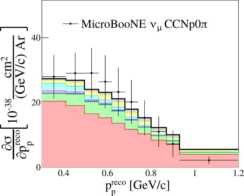
(a)

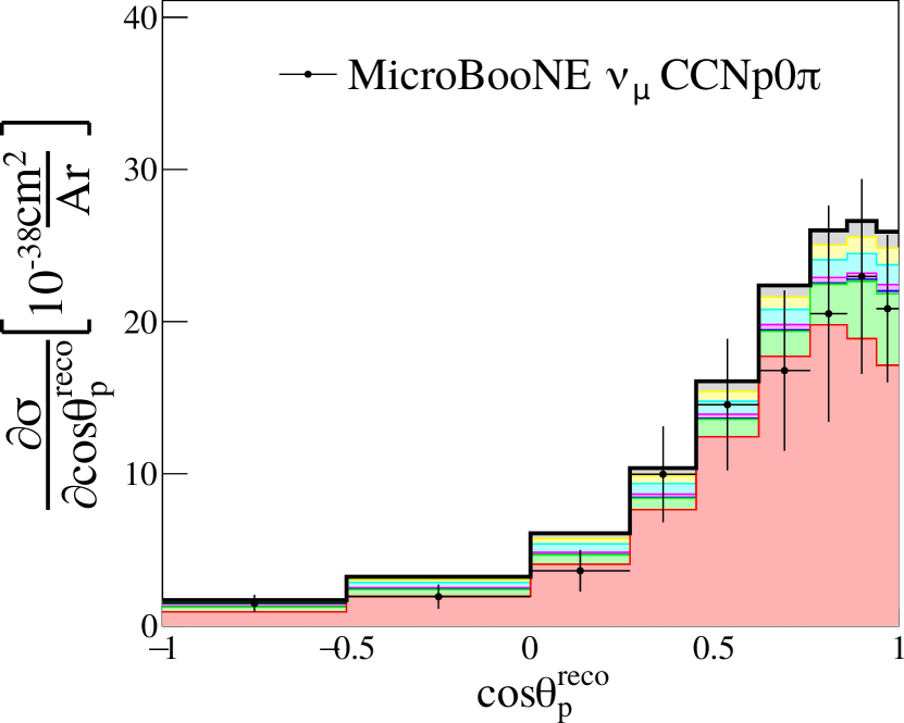
(b)

(c)

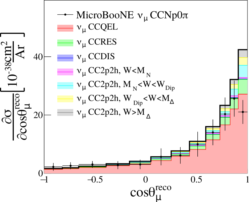
(d)

Figure 40: MicroBooNE $\nu_{\mu}$CCNp0$\pi$ flux-averaged differential cross section on ⁴⁰Ar as a function of muon and proton kinematics. The GENIE prediction is obtained with the G18_10a_02_11b tune. The nominal prediction is divided into interaction modes.

Appendix C Additional Nuclear Uncertainties

Here, we explore modeling aspects that were not included in the tuning exercise.

C.1 Nuclear model implementation

Uncertainties in the nuclear model affect the dynamics of the outgoing muon and nucleon after a QEL or a 2p2h interaction.

In the Valencia model implementation in GENIE, the differential cross section is evaluated at an effective energy transfer $\tilde{q}_{0}$, which takes into account the nucleon removal energy. The implementation in the QEL and 2p2h processes is slightly different. The effective energy transfer $\tilde{q}_{0}$ used in the Valencia QEL model implementation is:

$$\tilde{q}_{0}=q_{0}+E_{N_{i}}-E_{p}=E_{N_{f}}-E_{p}$$ (5)

$E_{N_{i}}$ is the energy of the off-shell initial nucleon, which is bound with a binding energy $E_{b}$. $E_{p}$ is the energy of the initial nucleon on-shell with a momentum $\mathbf{p}$, $E_{p}=\sqrt{M_{N}^{2}+\mathbf{p}^{2}}$. $E_{N_{f}}$ is the energy of the nucleon produced after the QEL interaction, which is on-shell. In other words, the effective energy transfer is reduced relative to the ordinary one by the amount of energy needed to put the initial nucleon on the mass shell. The binding energy and initial nucleon momentum are determined by the corresponding nuclear model. In this work, for QEL interactions we refer to $\tilde{q}_{0}$ as $\tilde{q}^{\text{QEL}}_{0}$. Notice that $\tilde{q}^{\text{QEL}}_{0}$ depends on the event kinematics.

In the Valencia 2p2h model implementation, the effective energy transfer is calculated as:

$$\tilde{q}_{0}=q_{0}-q^{\text{2p2h}}_{\text{shift}},\enskip\text{where}\enskip q^{\text{2p2h}}_{\text{shift}}\equiv M(A_{Z+1})-M(A_{Z}).$$

In this case, $q^{\text{2p2h}}_{\text{shift}}$ is independent of the event kinematics. For a carbon target, $q^{\text{2p2h}}_{\text{shift}}(^{12}\text{C})=16.8$ MeV, whilst $q^{\text{2p2h}}_{\text{shift}}(^{40}\text{Ar})=0.99$ MeV for argon.

Shifts on $\tilde{q}_{0}$ are effective modifications of the binding energy in the nuclear model. It is possible to apply relative shift to $\tilde{q}_{0}$ for both QEL and 2p2h calculations by modifying $q^{\text{QEL}}_{0}$ and $q^{\text{2p2h}}_{\text{shift}}$. This modification translates as:

$$\tilde{q}^{\text{QEL}}_{0}\rightarrow\tilde{q}^{\text{QEL}}_{0}(1+f^{\text{QEL}})$$

$$q^{\text{2p2h}}_{\text{shift}}\rightarrow q^{\text{2p2h}}_{\text{shift}}(1+f^{\text{2p2h}})$$

$f^{\text{QEL}}$ and $f^{\text{2p2h}}$ are two dimensionless parameters. In the GENIE v3 version, both parameters default to 0. Both $f^{\text{QEL}}$ and $f^{\text{2p2h}}$ parameters are included in the initial iteration of this analysis.

Ref. [74] suggests that shifts on $\tilde{q}^{\text{QEL}}_{0}$ ($q^{\text{2p2h}}_{\text{shift}}$) of $0-20$ MeV ($0-40$ MeV) for QEL (2p2h) are in reasonable agreement with electro-scattering data. The effect of such variations on the 2p2h cross-section prediction is shown in Fig. 41. The biggest variation is observed on $d\sigma/dQ^{2}$ for both QEL and 2p2h. For the 2p2h cross section, this systematic shifts peaks position in $W$.

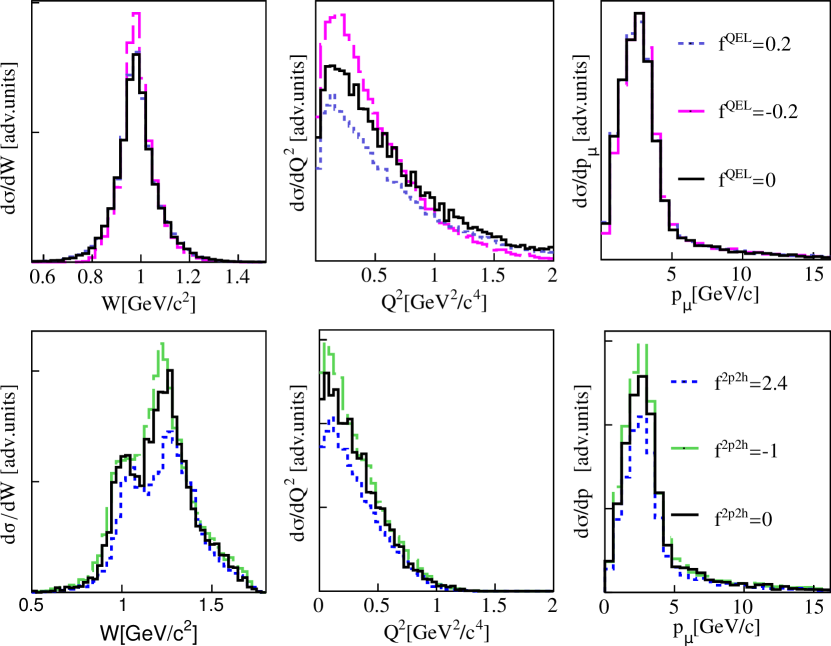
Figure 41: Flux-integrated differential $\nu_{\mu}^{12}$C CC2p2h cross section dependence with $W$, $Q^{2}$ or $p_{\mu}$. Events are generated with the G18_10a_02_11b tune and the NuMI $\nu_{\mu}$ low energy flux [8]. The top (bottom) three plots show the CCQEL (CC2p2h) differential cross section as a function of $W$, $Q^{2}$ or $p_{\mu}$. The black prediction corresponds to the GENIE v3 case, where no shifts on $\tilde{q}^{\text{QEL}}_{0}$ and $q^{\text{2p2h}}_{\text{shift}}$ are considered. The variations considered for the $f^{\text{QEL}}$ and $f^{\text{2p2h}}$ parameters correspond to an absolute shift to $\tilde{q}^{\text{QEL}}_{0}$ and $q^{\text{2p2h}}_{\text{shift}}$ of 20 MeV for QEL interactions and of 40 MeV for 2p2h interactions.

C.2 Final state interaction implementation

Final-state interactions (FSI) are crucial for modeling nuclear cross sections as they affect the event topology and kinematics of an event. There are different models available in GENIE to simulate FSI [14, 50]. In particular, G18_10a_02_11b models FSI with the INTRANUKE hA model [22].

INTRANUKE hA is an empirical model that considers a single interaction which is based on hadron-nucleus data [50]. In particular, pion-nucleus data are used to determine the inelastic (Inel), absorption (Abs), charge-exchange (CEx) and pion production ($\pi$Prod) fractions ($f_{i}$). The fractions depend on the pion kinetic energy and the nuclear atomic number. These fractions satisfy that $\sum_{i}f_{i}^{\pi^{\pm}}=1$ (unitarity condition), where $i$ is an index that runs over the available processes aforementioned.

Two parameters are introduced to be able to modify the $f_{\text{Abs}}^{\pi^{\pm}}$ and $f_{\text{Abs}}^{\pi^{0}}$ while preserving unitarity:

$$f_{\text{Abs}}^{{}^{\prime}\,\,\pi^{\pm}}=\frac{S_{\text{Abs}}^{\pi^{\pm}}\cdot f_{\text{Abs}}^{\pi^{\pm}}}{f_{\text{Inel}}^{\pi^{\pm}}+S_{\text{Abs}}^{\pi^{\pm}}\cdot f_{\text{Abs}}^{\pi^{\pm}}+f_{\text{CEx}}^{\pi^{\pm}}+f_{\pi\text{Prod}}^{\pi^{\pm}}}$$

The other fractions are also modified as a consequence of this scaling. Notice that variations of $S_{\text{Abs}}^{\pi^{\pm}}$ do not scale $f_{\text{Abs}}^{{}^{\prime}\,\,\pi^{\pm}}$ linearly.

Similarly, a scaling parameter is introduced to scale the charged pion mean-free path. This is referred to as $S_{\text{MFP}}^{\pi^{\pm}}$. The same approach can be applied to other processes and to nucleon fractions.

Figure 42 shows the dependence of each hA fraction as a function of the pion kinetic energy ($T_{\pi}$) for carbon and argon targets. The FSI fractions and their uncertainty are extracted from fits to hadron-nucleus scattering data [75, 50]. The uncertainty associated with $f_{\text{Abs}}^{\pi^{\pm}}$ is 15%.

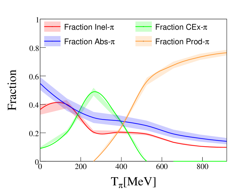
(a)

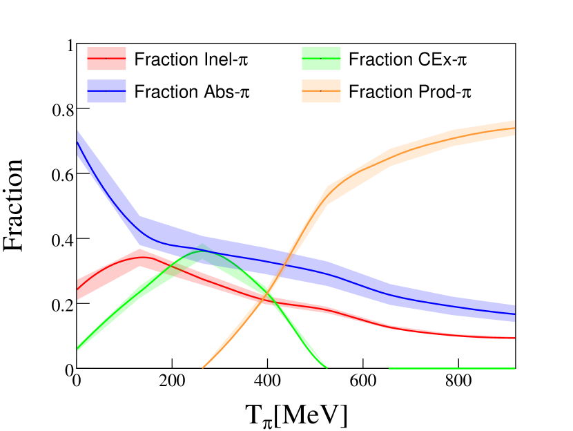
(b)

Figure 42: hA FSI pion fractions for (a) ¹²C and (b) ⁴⁰Ar as a function of the pion kinetic energy. The error bands represent the fraction variation when applying a $S_{\text{Abs}}^{\pi^{\pm}}=1.2$ on the pion absorption fraction, which corresponds to a variation of $\sim 15$% for the pion absorption fraction on carbon at $T_{\pi}=200$ MeV.

Variations of the FSI parameters considered in this work result in the migration of CC1$\pi$ events into the CC0$\pi$ sample. The effect on the prediction depends on the topology definition. For CC0$\pi$ samples, it mostly affects the overall normalization of the cross-section. The measurement most sensitive to this variation is the $\nu_{\mu}$ CCNp0$\pi$ MINER$\nu$A differential cross section as a function of $\delta\alpha_{T}$, see Fig. 43. A decrease in $S_{\text{Abs}}^{\pi^{\pm}}$ reduces the cross section at $\delta\alpha_{T}\sim 180^{\circ}$. In addition, this model variation also affects the slope of the distribution.

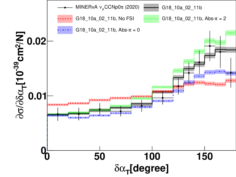
Figure 43: Impact of $S_{\text{Abs}}^{\pi^{\pm}}$ on MINER$\nu$A CCNp0$\pi$ flux-integrated differential cross section predictions as a function of $\delta\alpha_{T}$.

In this tune, only parameters related to charged pion absorption are included: $S_{\text{Abs}}^{\pi^{\pm}}$ and $S_{\text{MFP}}^{\pi^{\pm}}$. Pion inelastic fractions are not relevant at the energies of interest for this work. Nucleon FSI parameters are relevant for the study of exclusive cross-section measurements with protons in the final state. Ideally, to perform a global tune with CC0$\pi$ and CCNp0$\pi$ data, nucleon FSI parameters must be considered in the analysis. Including these parameters in the analysis substantially increases the computing time. In addition, it is desirable to first understand the tensions between CC0$\pi$ and CCNp0$\pi$ measurements. Therefore, it is therefore convenient to reduce the complexity of the analysis and focus on CC0$\pi$ datasets only. Nucleon FSI parameters will be included in future iterations of this work.

C.3 Final choice of parameters for the CC0$\pi$ tune

A series of preliminary tunes were performed using different priors or parameter sets. The goal of this study is to determine which parameters to include in the final tune.

Nuclear effects in the QEL cross section are tweaked with the RPA parametrization. Free-nucleon cross-section data suggests that the QEL cross section should not be scaled. This condition can be incorporated in our analysis by imposing a more restrictive prior on $S_{\text{RPA}}$ of $\sigma_{S}=0.01$. Tunes performed using this prior result in worse goodness of fit, suggesting that a less restrictive prior on the sum is desired to improve the agreement with the data. This motivated our choice for a prior on the sum of $\sigma_{S}=0.2$, as described in Sec. III.1.

FSI interactions are important to describe CC0$\pi$ measurements. Additional parameters must be consistent with previous data [50], making this tricky. The results of test cases with FSI suggest that variations of these parameter that respect pion-nucleus scattering data do not have a big impact on the tune results. Consequently, these parameters are not included in the final analysis.

Various choices were made to get a more representative result. Although full coverage in parameters can be sought, that is not always possible or desirable. For this study, Professor allows a large parameter set which don’t have to be ReWeight variables. A study of the $f^{\text{QEL}}$ and $f^{\text{2p2h}}$ parameters in the tune was made. Strong correlations are observed between the $f^{\text{QEL}}$, $f^{\text{2p2h}}$ and $\omega_{\text{RPA}}$ and $S^{\text{2p2h}}$ parameters. In some cases, these correlations lead to unphysical values for $f^{\text{QEL}}$ and $f^{\text{2p2h}}$. For this reason, these parameters are excluded from the analysis.

The final-parameter set used in this work is summarized in Tab. 3.

MC

Monte Carlo

SM

Standard Model

CKM

Cabibbo-Kobayashi-Maskawa

CC

Charged-Current

NC

Neutral-Current

QEL

Quasi-ELastic

RES

REsonance Scattering

DoF

Degree of Freedom

NRB

Non-Resonant Background

2p2h

Two-particles–two-holes

SIS

Shallow-Inelastic Scattering

DIS

Deep-Inelastic Scattering

FSI

Final-State Interactions

QCD

Quantum-ChromoDynamics

RFG

Relativistic Fermi Gas

LFG

Local Fermi Gas

CFG

Correlated Fermi Gas

RPA

Random-Phase Approximation

AGKY

Andreopoulos-Gallagher-Kehayias-Yang

CMC

Comprehensive Model Configuration

CMCs

Comprehensive Model Configurations

STKI

Single-Transverse Kinematic Imbalance

BNB

Booster Neutrino Beam

NuMI

Neutrino at the Main Injector

FHC

Forward Horn Current

RHC

Reverse Horn Current

LArTPC

Liquid Argon Time Projection Chamber

PPP

Peele’s Pertinent Puzzle

NS

Norm-Shape

PID

Particle IDentification

References

- Aguilar-Arevalo et al. [2009a] A. A. Aguilar-Arevalo et al. (MiniBooNE Collaboration), The MiniBooNE detector, Nucl. Instrum. Meth. A 599, 28 (2009a), 0806.4201 [hep-ex] .
- Abe et al. [2011] K. Abe et al. (T2K Collaboration), The T2K experiment, Nucl. Instrum. Meth. A 659, 106 (2011), 1106.1238 [physics.ins-det] .
- Acciarri et al. [2017a] R. Acciarri et al., Design and construction of the MicroBooNE detector, JINST 12, P02017 (2017a), 1612.05824 [physics.ins-det] .
- Ascencio et al. [2022] M. V. Ascencio et al. (MINERA Collaboration), Measurement of inclusive charged-current scattering on hydrocarbon at GeV with low three-momentum transfer, Phys. Rev. D 106, 032001 (2022), 2110.13372 [hep-ex] .
- Tena-Vidal et al. [2021] J. Tena-Vidal et al. (GENIE Collaboration), Neutrino–nucleon cross-section model tuning in GENIE v3, Phys. Rev. D 104, 072009 (2021), 2104.09179 [hep-ph] .
- Abe et al. [2013] K. Abe et al. (T2K Collaboration), T2K neutrino flux prediction, Phys. Rev. D 87, 012001 (2013), [Addendum: ibid. 87, 019902 (2013)], 1211.0469 [hep-ex] .
- Aguilar-Arevalo et al. [2009b] A. A. Aguilar-Arevalo et al. (MiniBooNE Collaboration), Neutrino flux prediction at MiniBooNE, Phys. Rev. D 79, 072002 (2009b), 0806.1449 [hep-ex] .
- Aliaga et al. [2016] L. Aliaga et al. (MINERA Collaboration), Neutrino flux predictions for the numi beam, Phys. Rev. D 94, 092005 (2016), 1607.00704 [hep-ex] .
- Tena-Vidal et al. [2022] J. Tena-Vidal et al. (GENIE Collaboration), Hadronization model tuning in GENIE v3, Phys. Rev. D 105, 012009 (2022), 2106.05884 [hep-ph] .
- Abratenko et al. [2022] P. V. Abratenko et al. (MicroBooNE Collaboration), New GENIE model tune for MicroBooNE, Phys. Rev. D 105, 072001 (2022), 2110.14028 [hep-ex] .
- Filkins et al. [2020] A. Filkins et al. (MINERA Collaboration), Double-differential inclusive charged-current cross sections on hydrocarbon in MINERA at GeV, Phys. Rev. D 101, 112007 (2020), 2002.12496 [hep-ex] .
- Abe et al. [2021a] K. Abe et al. (T2K Collaboration), Improved constraints on neutrino mixing from the T2K experiment with protons on target, Phys. Rev. D 103, 112008 (2021a), 2101.03779 [hep-ex] .
- Nieves et al. [2011] J. Nieves, I. Ruiz Simo, and M. J. Vicente Vacas, Inclusive charged-current neutrino–nucleus reactions, Phys. Rev. C 83, 045501 (2011), 1102.2777 [hep-ph] .
- Alvarez-Ruso et al. [2021] L. Alvarez-Ruso et al. (GENIE Collaboration), Recent highlights from GENIE v3, Eur. Phys. J. ST 230, 4449 (2021), 2106.09381 [hep-ph] .
- Nieves et al. [2004] J. Nieves, J. E. Amaro, and M. Valverde, Inclusive quasielastic charged-current neutrino–nucleus reactions, Phys. Rev. C 70, 055503 (2004), [Erratum: ibid. 72, 019902 (2005)], arXiv:nucl-th/0408005 .
- Kovalenko [1990] S. G. Kovalenko, Quasielastic neutrino production of charmed baryons from the point of view of local duality, Sov. J. Nucl. Phys. 52, 934 (1990), [Yad. Fiz. 52, 1478 (1990)].
- Pais [1971] A. Pais, Weak interactions at high energies, Annals Phys. 63, 361 (1971).
- Berger and Sehgal [2007] C. Berger and L. M. Sehgal, Lepton mass effects in single pion production by neutrinos, Phys. Rev. D 76, 113004 (2007), [Erratum: ibid. 77, 059901(E) (2008)], 0709.4378 [hep-ph] .
- Bodek and Yang [2002] A. Bodek and U.-K. Yang, Modeling deep inelastic cross sections in the few GeV region, Nucl. Phys. B (Proc. Suppl.) 112, 70 (2002), Proceedings of the 1st International Workshop on Neutrino–Nucleus Interactions in the Few GeV Region (NuInt 2001), Tsukuba, Japan, December 13–16, 2001, arXiv:hep-ex/0203009 .
- Aivazis et al. [1991] M. A. G. Aivazis, W.-K. Tung, and F. I. Olness, Next-to-Leading Order QCD formulation of deep inelastic scattering, in Proceedings of the Meeting of the Division of Particles & Fields of the APS (Particles & Fields 1991), Vancouver, British Columbia, Canada, August 18 – 22, 1991 (1991) pp. 663–665, arXiv:hep-ph/9302305 .
- Yang et al. [2009] T. Yang et al., A hadronization model for few-GeV neutrino interactions, Eur. Phys. J. C 63, 1 (2009), 0904.4043 [hep-ph] .
- [22] C. Andreopoulos et al., The GENIE neutrino Monte Carlo generator: Physics & user manual (version 2.10.0), 1510.05494 [hep-ph] .
- Alcaraz-Aunion and Walding [2009] J. L. Alcaraz-Aunion and J. Walding, Measurement of the -CCQE cross section in the SciBooNE experiment, AIP Conf. Proc. 1189, 145 (2009), Proceedings of the 6th International Workshop on Neutrino–Nucleus Interactions in the Few GeV Region (NuInt 2009), Sitges, Barcelona, Spain, May 18–22, 2009, 0909.5647 [hep-ex] .
- Lyubushkin et al. [2009] V. V. Lyubushkin et al. (NOMAD Collaboration), A study of quasi-elastic muon neutrino and antineutrino scattering in the NOMAD experiment, Eur. Phys. J. C 63, 355 (2009), 0812.4543 [hep-ex] .
- Aguilar-Arevalo et al. [2010] A. A. Aguilar-Arevalo et al. (MiniBooNE Collaboration), First measurement of the muon neutrino charged current quasielastic double differential cross section, Phys. Rev. D 81, 092005 (2010), 1002.2680 [hep-ex] .
- Aguilar-Arevalo et al. [2013] A. A. Aguilar-Arevalo et al. (MiniBooNE Collaboration), First measurement of the muon antineutrino double-differential charged-current quasielastic cross section, Phys. Rev. D 88, 032001 (2013), 1301.7067 [hep-ex] .
- Abe et al. [2018] K. Abe et al. (T2K Collaboration), Characterization of nuclear effects in muon-neutrino scattering on hydrocarbon with a measurement of final-state kinematics and correlations in charged-current pionless interactions at T2K, Phys. Rev. D 98, 032003 (2018), 1802.05078 [hep-ex] .
- Ruterbories et al. [2019] D. G. Ruterbories et al. (MINERA Collaboration), Measurement of quasielastic-like neutrino scattering at GeV on a hydrocarbon target, Phys. Rev. D 99, 012004 (2019), 1811.02774 [hep-ex] .
- Lu et al. [2018] X.-G. Lu et al. (MINERA Collaboration), Measurement of final-state correlations in neutrino muon–proton mesonless production on hydrocarbon at GeV, Phys. Rev. Lett. 121, 022504 (2018), 1805.05486 [hep-ex] .
- Cai et al. [2020] T. Cai et al. (MINERA Collaboration), Nucleon binding energy and transverse momentum imbalance in neutrino–nucleus reactions, Phys. Rev. D 101, 092001 (2020), 1910.08658 [hep-ex] .
- Abratenko et al. [2020a] P. V. Abratenko et al. (MicroBooNE Collaboration), First measurement of differential charged current quasielasticlike –argon scattering cross sections with the MicroBooNE detector, Phys. Rev. Lett. 125, 201803 (2020a), 2006.00108 [hep-ex] .
- Abratenko et al. [2020b] P. V. Abratenko et al. (MicroBooNE Collaboration), Measurement of differential cross sections for –Ar charged-current interactions with protons and no pions in the final state with the MicroBooNE detector, Phys. Rev. D 102, 112013 (2020b), 2010.02390 [hep-ex] .
- Carneiro et al. [2020] M. F. Carneiro et al. (MINERA Collaboration), High-statistics measurement of neutrino quasielasticlike scattering at GeV on a hydrocarbon target, Phys. Rev. Lett. 124, 121801 (2020), 1912.09890 [hep-ex] .
- Ruterbories et al. [2022] D. G. Ruterbories et al. (MINERA Collaboration), Simultaneous measurement of proton and lepton kinematics in quasielasticlike –hydrocarbon interactions from to GeV, Phys. Rev. Lett. 129, 021803 (2022), 2203.08022 [hep-ex] .
- Abe et al. [2020a] K. Abe et al. (T2K Collaboration), First measurement of the charged current double-differential cross section on a water target without pions in the final state, Phys. Rev. D 102, 012007 (2020a), 1908.10249 [hep-ex] .
- Abe et al. [2020b] K. Abe et al. (T2K Collaboration), First combined measurement of the muon neutrino and antineutrino charged-current cross section without pions in the final state at T2K, Phys. Rev. D 101, 112001 (2020b), 2002.09323 [hep-ex] .
- Abe et al. [2021b] K. Abe et al., Measurements of and charged-current cross-sections without detected pions or protons on water and hydrocarbon at a mean anti-neutrino energy of GeV, Prog. Theor. Exp. Phys. 2021, 043C01 (2021b), 2004.13989 [hep-ex] .
- Patrick et al. [2018] C. E. Patrick et al. (MINERA Collaboration), Measurement of the muon antineutrino double-differential cross section for quasielastic-like scattering on hydrocarbon at GeV, Phys. Rev. D 97, 052002 (2018), 1801.01197 [hep-ex] .
- Avanzini et al. [2022] M. B. Avanzini et al., Comparisons and challenges of modern neutrino-scattering experiments, Phys. Rev. D 105, 092004 (2022), 2112.09194 [hep-ex] .
- Lu et al. [2016] X.-G. Lu et al., Measurement of nuclear effects in neutrino interactions with minimal dependence on neutrino energy, Phys. Rev. C 94, 015503 (2016), 1512.05748 [nucl-th] .
- Abe et al. [2016] K. Abe et al. (T2K Collaboration), Measurement of double-differential muon neutrino charged-current interactions on without pions in the final state using the T2K off-axis beam, Phys. Rev. D 93, 112012 (2016), 1602.03652 [hep-ex] .
- Meyer et al. [2016] A. S. Meyer et al., Deuterium target data for precision neutrino–nucleus cross sections, Phys. Rev. D 93, 113015 (2016), 1603.03048 [hep-ph] .
- Valverde et al. [2006] M. Valverde, J. E. Amaro, and J. Nieves, Theoretical uncertainties on quasielastic charged-current neutrino–nucleus cross sections, Phys. Lett. B 638, 325 (2006), arXiv:hep-ph/0604042 .
- [44] R. Gran, Model uncertainties for Valencia RPA effect for MINERA, 1705.02932 [hep-ex] .
- Rodrigues et al. [2016] P. A. Rodrigues et al. (MINERA Collaboration), Identification of nuclear effects in neutrino–carbon interactions at low three-momentum transfer, Phys. Rev. Lett. 116, 071802 (2016), [Addendum: ibid. 121, 209902 (2018)], 1511.05944 [hep-ex] .
- Dolan et al. [2020] S. Dolan, G. D. Megias, and S. Bolognesi, Implementation of the SuSAv2-meson exchange current and models in GENIE and analysis of nuclear effects in T2K measurements, Phys. Rev. D 101, 033003 (2020), 1905.08556 [hep-ex] .
- Freedman et al. [1982] R. A. Freedman, G. A. Miller, and E. M. Henley, Isobar dynamics and pion–nucleus elastic scattering, Nucl. Phys. A 389, 457 (1982).
- Moniz et al. [1971] E. J. Moniz et al., Nuclear Fermi momenta from quasielastic electron scattering, Phys. Rev. Lett. 26, 445 (1971).
- Benhar et al. [1994] O. Benhar, A. Fabrocini, S. Fantoni, and I. Sick, Spectral function of finite nuclei and scattering of GeV electrons, Nucl. Phys. A 579, 493 (1994).
- Dytman et al. [2021] S. A. Dytman et al., Comparison of validation methods of simulations for final state interactions in hadron production experiments, Phys. Rev. D 104, 053006 (2021), 2103.07535 [hep-ph] .
- Chakrani et al. [2022] J. Chakrani, M. Buizza Avanzini, and S. Dolan, Parametrising CCQE uncertainties in the Spectral Function model for neutrino oscillation analyses, PoS NuFact2021, 235 (2022), Proceedings of the 22nd International Workshop on Neutrinos from Accelerators (NuFact 2021), Cagliari, Italy, September 6–11, 2021, 2202.03219 [hep-ph] .
- Bonus et al. [2020] T. Bonus, J. T. Sobczyk, M. Siemaszko, and C. Juszczak, Data-based two-body current contribution to the neutrino–nucleus cross section, Phys. Rev. C 102, 015502 (2020), 2003.00088 [hep-ex] .
- Hanson et al. [2005] K. M. Hanson, T. Kawano, and P. Talou, Probabilistic interpretation of Peelle’s Pertinent Puzzle and its resolution, AIP Conf. Proc. 769, 304 (2005), Proceedings of the International Conference on Nuclear Data for Science and Technology (ND 2004), Santa Fe, New Mexico, USA, 26 September – 1 October 2004.
- D’Agostini [1994] G. D’Agostini, On the use of the covariance matrix to fit correlated data, Nucl. Instrum. Meth. A 346, 306 (1994).
- Buckley et al. [2010] A. Buckley et al., Systematic event generator tuning for the LHC, Eur. Phys. J. C 65, 331 (2010), 0907.2973 [hep-ph] .
- Bourguille et al. [2021] B. Bourguille, J. Nieves, and F. Sánchez, Inclusive and exclusive neutrino–nucleus cross sections and the reconstruction of the interaction kinematics, JHEP 04, 004 (2021), 2012.12653 [hep-ph] .
- Meyer et al. [2022] A. S. Meyer, A. Walker-Loud, and C. Wilkinson, Status of Lattice QCD determination of nucleon form factors and their relevance for the few-GeV neutrino program, Ann. Rev. Nucl. Part. Sci. 72, 1–30 (2022), 2201.01839 [hep-lat] .
- Niewczas and Sobczyk [2019] K. Niewczas and J. T. Sobczyk, Nuclear transparency in Monte Carlo neutrino event generators, Phys. Rev. C 100, 015505 (2019), 1902.05618 [hep-ex] .
- [59] S. Dolan, Exploring nuclear effects in neutrino–nucleus interactions using measurements of transverse kinematic imbalance from T2K and MINERA, 1810.06043 [hep-ex] .
- Garino et al. [1992] G. Garino et al., Proton propagation in nuclei studied in the reaction, Phys. Rev. C 45, 780 (1992).
- O’Neill et al. [1995] T. G. O’Neill et al., -dependence of nuclear transparency in quasielastic at high , Phys. Lett. B 351, 87 (1995).
- Dutta et al. [2003] D. Dutta et al., Quasielastic reaction on , , and , Phys. Rev. C 68, 064603 (2003), arXiv:nucl-ex/0303011 .
- Rohe et al. [2005] D. Rohe et al. (E97-006 Collaboration), Nuclear transparency from quasielastic , Phys. Rev. C 72, 054602 (2005), arXiv:nucl-ex/0506007 .
- Ershova et al. [2022] A. Ershova et al., Study of final-state interactions of protons in neutrino–nucleus scattering with INCL and NuWro cascade models, Phys. Rev. D 106, 032009 (2022), 2202.10402 [hep-ph] .
- Nikolakopoulos et al. [2022] A. Nikolakopoulos et al., Benchmarking intra-nuclear cascade models for neutrino scattering with relativistic optical potentials, Phys. Rev. C 105, 054603 (2022), 2202.01689 [nucl-th] .
- Aliaga et al. [2014] L. Aliaga et al. (MINERA Collaboration), Design, calibration, and performance of the MINERA detector, Nucl. Instrum. Meth. A 743, 130 (2014), 1305.5199 [physics.ins-det] .
- Lu et al. [2021] X.-G. Lu et al. (MINERA Collaboration), Exploring neutrino–nucleus interactions in the GeV regime using MINERA, Eur. Phys. J. ST 230, 4243 (2021), 2107.02064 [hep-ex] .
- Michael et al. [2008] D. G. Michael et al. (MINOS Collaboration), The magnetized steel and scintillator calorimeters of the MINOS experiment, Nucl. Instrum. Meth. A 596, 190 (2008), 0805.3170 [physics.ins-det] .
- Acciarri et al. [2017b] R. Acciarri et al. (MicroBooNE Collaboration), Noise characterization and filtering in the MicroBooNE Liquid Argon TPC, JINST 12, P08003 (2017b), 1705.07341 [physics.ins-det] .
- Adams et al. [2018] C. Adams et al. (MicroBooNE Collaboration), Ionization electron signal processing in single phase LArTPCs. Part II. Data/simulation comparison and performance in MicroBooNE, JINST 13, P07007 (2018), 1804.02583 [physics.ins-det] .
- Acciarri et al. [2018] R. Acciarri et al., The Pandora multi-algorithm approach to automated pattern recognition of cosmic-ray muon and neutrino events in the MicroBooNE detector, Eur. Phys. J. C 78, 82 (2018), 1708.03135 [hep-ex] .
- Abratenko et al. [2019] P. V. Abratenko et al. (MicroBooNE Collaboration), First measurement of inclusive muon neutrino charged current differential cross sections on argon at GeV with the MicroBooNE detector, Phys. Rev. Lett. 123, 131801 (2019), 1905.09694 [hep-ex] .
- Adams et al. [2019] C. Adams et al. (MicroBooNE Collaboration), First measurement of charged-current production on argon with the MicroBooNE detector, Phys. Rev. D 99, 091102 (2019), 1811.02700 [hep-ex] .
- Bodek and Cai [2019] A. Bodek and T. Cai, Removal energies and final state interaction in lepton nucleus scattering, Eur. Phys. J. C 79, 293 (2019), 1801.07975 [nucl-th] .
- Pinzon Guerra et al. [2019] E. S. Pinzon Guerra et al., Using world –nucleus scattering data to constrain an intranuclear cascade model, Phys. Rev. D 99, 052007 (2019), 1812.06912 [hep-ex] .