Dynamical detection of mean-field topological phases in an interacting Chern insulator
Abstract
Interactions generically have important effects on the topological quantum phases. For a quantum anomalous Hall (QAH) insulator, the presence of interactions can qualitatively change the topological phase diagram which, however, is typically hard to measure in the experiment. Here we propose a novel scheme based on quench dynamics to detect the mean-field topological phase diagram of an interacting Chern insulator described by QAH-Hubbard model, with nontrivial dynamical quantum physics being uncovered. We focus on the dynamical properties of the system at a weak to intermediate Hubbard interaction which mainly induces a ferromagnetic order under the mean-field level. Remarkably, three characteristic times , , and are found in the quench dynamics. The first two capture the emergence of dynamical self-consistent particle density and dynamical topological phase transition respectively, while the last one gives a linear scaling time on the topological phase boundaries. A more interesting result is that () occurs in repulsive (attractive) interaction and the Chern number is determined by any two characteristic time scales when the system is quenched from an initial nearly fully polarized state to the topologically nontrivial regimes, showing a dynamical way to determine equilibrium mean-field topological phase diagram via the time scales. Experimentally, the measurement of is challenging while and can be directly readout by measuring the spin polarizations of four Dirac points and the time-dependent particle density, respectively. Our work reveals the novel interacting effects on the topological phases and shall promote the experimental observation.
I Introduction
Topological quantum phase is currently a mainstream of research in condensed matter physics [1, 2, 3, 4, 5]. At equilibrium, the topological phases can be characterized by nonlocal topological invariants [6, 7] defined in ground states. This classifies the gapped band structures into distinct topological states, with great success having been achieved in study of topological insulators [8, 9, 10, 11], topological semimetals [12, 13, 14, 15], and topological superconductors [16, 17, 18, 19, 20]. Nevertheless, this noninteracting topological phase can be greatly affected after considering many-body interaction [21, 22, 23, 24, 25, 26, 27, 28, 29, 30, 31, 32]. For instance, the repulsive Hubbard interaction can drive a trivial insulator into a topological Mott insulator [33, 34, 35], while the attractive Hubbard interaction may drive a trivial phase of two-dimensional (2D) quantum anomalous Hall (QAH) system into a topological superconductor/superfluid [36, 37, 38, 39]. Hence how to accurately identify the topological phases driven by the interactions is still a fundamental issue and usually hard in experiments.
In recent years, the rapid development of quantum simulations [40, 41, 42] provides new realistic platforms to explore exotic interacting physics, such as ultracold atoms in optical lattices [43, 44, 45, 46, 47, 48, 49] and superconducting qubits [50, 51, 52]. A number of topological models have been realized in experiments, such as the 1D Su-Schriffer-Heeger model [53, 54], 1D AIII class topological insulator [55, 56], 1D bosonic symmetry-protected phase [57, 58], 2D Haldane model [59], the spin-orbit coupled QAH model [60, 61, 62], and the 3D Weyl semimetal band [63, 64, 65, 66, 67]. Accordingly, the various detection schemes for the exotic topological physics are also developed, ranging from the measurements of equilibrium topological physics [68, 69, 70, 71] to non-equilibrium quantum dynamics [72, 73, 74, 75, 76, 77, 78, 79, 80, 81]. In particular, the dynamical characterization [82, 83, 84, 85, 86, 87, 88] shows the correspondence between broad classes of equilibrium topological phases and the emergent dynamical topology in far-from-equilibrium quantum dynamics induced by quenching such topological systems, which brings about the systematic and high-precision schemes to detect the topological phases based on quantum dynamics and has advanced broad studies in experiment [89, 90, 91, 92, 93, 94, 95, 96, 97, 98]. Nevertheless, these current studies have been mainly focused on the noninteracting topological systems, while the particle-particle interactions are expected to have crucial effects on the topological phases, whose detection is typically hard to achieve. For example, when quenching an interacting topological system [99, 100, 101, 102], both the interactions and many-body states of the system evolve simultaneously after quenching, leading to complex nonlinear quantum dynamics [103, 104, 105, 106] and exotic nonequilibrium phenomena [107, 108, 109, 110]. With above considerations, there are two nontrivial issues for the quantum dynamics in the interacting Chern insulator that have not been studied: (i) how the dynamical properties change when the Hubbard interaction is added into the Chern insulator and performing quench dynamics? (ii) is there any universal feature in the dynamical evolution to characterize the equilibrium mean-field topological phases?
In this paper, we address these issues and propose a novel scheme based on quench dynamics to detect the mean-field topological phase diagram of an interacting Chern insulator described by QAH-Hubbard model, with nontrivial dynamical quantum physics being uncovered. Specifically, we consider a 2D QAH system in presence of a weak to intermediate Hubbard interaction which mainly induces a ferromagnetic order under the mean-field level. By quenching the system from an initial nearly fully polarized trivial state to a parameter regime in which the equilibrium phase is topologically nontrivial, we uncover two dynamical phenomena rendering the dynamical signals of the equilibrium mean-field phase. First, there are three characteristic times , , and , capturing the dynamical self-consistent particle density, dynamical topological phase transition, and the linear scaling time on the topological phase boundaries, respectively. Second, () occurs in the repulsive (attractive) interaction and the Chern number is determined by any two characteristic time scales. Based on these two fundamental properties, we can easily determine the equilibrium mean-field topological phase diagram by comparing any two time scales. Experimentally, the measurement of is challenging while and can be directly readout by measuring the spin polarizations of four Dirac points and the time-dependent particle density respectively. This result provides a dynamical detection scheme with high feasibility and simplicity for measuring the mean-field topological phase diagram in interacting systems, which may be applied to the recent quantum simulation experiments.
The remaining part of this paper is organized as follows. In Sec. II, we introduce the QAH-Hubbard model. In Sec. III, we study the quench dynamics of the system. In Sec. IV, we reveal the nontrivial dynamical properties in quench dynamics. In Sec. V, we determine the mean-field topological phase diagram via the time scales. In Sec. VI, we propose the experimental detection scheme for the equilibrium mean-field topological phases. Finally, we summarize the main results and provide the brief discussion in Sec. VII.
II QAH-Hubbard model
Our starting point is a minimal 2D QAH model [36, 38], which has been recently realized in cold atoms [60, 89, 91, 62], together with an attractive or repulsive on-site Hubbard interaction of strength . The system is now described by the QAH-Hubbard Hamiltonian
| (1) | ||||
where is the spinor operator of momentum , with or is the particle number operator at site , are the Pauli matrices, and is the Zeeman coupling. Here and are the spin-conserved and spin-flipped hopping coefficients, respectively. In the noninteracting case, the Bloch Hamiltonian produces two energy bands , for which the gap can be closed at Dirac points with , , , and for certain Zeeman coupling. When the system is fully gapped, the corresponding band topology can be characterized by the first Chern number , determining the QAH topological region with and the trivial region . This noninteracting topological property can also be captured by the intuitive physical quantities, such as the numbers of edge states [36], the spin textures on band inversion surfaces [82, 91], and the spin polarizations at four Dirac points [68, 60].
The presence of nonzero interactions can greatly affect the physics of Hamiltonian (1) and may induce various interesting quantum phases at suitable interaction strength, such as the superfluid phase in attractive interaction [111, 112] and the antiferromagnetic phase in repulsive interaction [113, 114]. Especially for a general strong interaction, the system may host rich magnetic phases [115, 116, 117]. Here we focus on the 2D system at half filling within a weak to intermediate interacting regime, where the interaction mainly induces ferromagnetic order [118]. For this 2D case, the Hubbard interaction can be still treated by employing the mean field theory, in which the fluctuations around the average value of the order parameter are small and can be neglected [37, 38, 39, 104, 105, 106]. Accordingly, the Hubbard interaction term is rewritten as
| (2) |
with . Here is the total number of sites. It is clear that the nonzero interaction corrects the Zeeman coupling to an effective form
| (3) |
where is the difference of density for spin-up and spin-down particles. The effective Zeeman coupling shifts the topological region to with in the interacting regime.
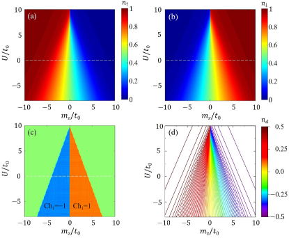
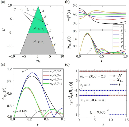
By self-consistently calculating the particle density [see Figs. 1(a) and 1(b)], the mean-field phase diagram of the QAH-Hubbard model (1) is shown in Fig. 1(c). We find an important feature that the topological phase boundaries depend on the strength of nonzero interaction and the Zeeman coupling linearly [see Appendix A]. Indeed, this linear behavior of topological boundaries is essentially a natural consequence of the linear form of the contour lines of in terms of the interaction strength and Zeeman coupling, as we show in Fig. 1(d). On these lines, is also unchanged, since is fully determined by the effective Zeeman coupling. Specifically, we have on the topological phase boundaries for . This linear scaling form of greatly affects the dynamical properties of the system and leads to novel phenomena in the quench dynamics, as we show in Sec. IV.
III Quench dynamics
Quantum quench dynamics has been widely used in cold atoms [61, 89, 119, 66]. We shall show that the above equilibrium mean-field phase diagram can be dynamically characterized and detected by employing the quantum quench scheme. Unlike the interaction quench in Refs. [103, 105], here we choose the Zeeman coupling as quench parameter, which has the following advantages: (i) The effective Zeeman coupling directly determines the topology of mean-field ground states at equilibrium; (ii) The Zeeman field in spin-orbit coupled quantum gases is controlled by the laser intensity and/or detuning and can be changed in a very short time scale, fulfilling the criterion for a sudden quench; (iii) The realistic experiments [120, 121, 122] have demonstrated that both the magnitude and the sign of Zeeman field can be tuned, which is more convenient to operate.
The quench protocol is as follows. First, we initialize the system into a nearly fully polarized state for time by taking a very large constant magnetization along the axis but a very small along axis. In this case the effect of interaction can be ignored, and the spin of initial state is almost along the axis with only a very small component in the - plane. At , we suddenly change the Zeeman coupling to the post-quenched value and remove . And then, the nearly fully polarized state begins to evolve under the equation of motion with the post-quenched Hamiltonian
| (4) |
where is instantaneous many-body state. We emphasize should have the same sign as the post-quenched in order to facilitate the capture of nontrivial properties in quantum dynamics. Also, all physics in the dynamics are robust against the tiny changes of the initial state.
In the progress of quench dynamics, we observe that the many-body state and the post-quenched Hamiltonian are both time-evolved, where the instantaneous particle density is time-dependent and determined as
| (5) |
This dynamic behavior is completely different from the noninteracting quantum quenches, where the post-quenched Hamiltonian keeps unchanged [82, 83, 84, 85, 86, 87]. Even if the post-quenched Hamiltonian may become steady after the long time evolution, it is still different from the equilibrium mean-field Hamiltonian with the post-quenched and , i.e.,
| (6) |
Here is the equilibrium value as we show in the Section II. Clearly, the novel dynamical evolution shows that the detection schemes for the noninteracting topological phases are inapplicable in this interacting case.
Next we employ the nontrivial characteristic time emerged in the above dynamical evolution to identify the mean-field topological phases. By defining the quantity , the time-dependent effective Zeeman coupling is given by
| (7) |
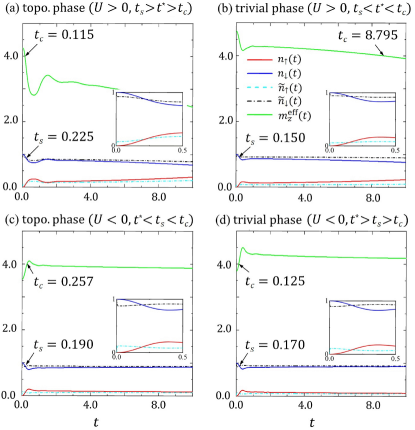
Their dynamical properties are shown in Fig. 2, where in a short-time evolution increases (decays) from an initial () when the post-quenched Zeeman coupling is positive (negative). It should be noted that now determines the topological number of post-quenched Hamiltonian through the relation for and otherwise. Considering that the topology of equilibrium mean-field Hamiltonian (6) is actually determined by its self-consistent particle density , a idea of capturing the equilibrium mean-field topological phases is to find a characteristic time in this dynamics such that
| (8) |
which gives a dynamical self-consistent particle density to characterize the equilibrium self-consistent particle density. Now this post-quenched Hamiltonian at is equivalent to the equilibrium mean-field Hamiltonian, and both of them host the same ground states. Accordingly, determines the topology of the equilibrium mean-field Hamiltonian. On the other hand, we introduce a characteristic time such that
| (9) |
characterizing the critical time of the dynamical topological phase transition of post-quenched Hamiltonian. Meanwhile, a nontrivial relation happens on the topological phase boundaries, giving . We remark this characteristic time on these topological boundaries as such that
| (10) |
which holds a unique value for the system with a fixed spin-orbit coupled strength due to the linear scaling of [see Fig. 1(d)]. With these three characteristic time scales , , and , the properties of equilibrium mean-field Hamiltonian can be completely characterized, where the ground states, the topological phase transition, and the topological phase boundaries are characterized by , , and respectively. In Fig. 2, we show that both and emerge in the short-time evolution. Together with in Fig. 5(b), we clearly observe that the relative time scales behave differently for the different equilibrium mean-field phases. This result provides a basic idea to establish the topological characterization and to detect the mean-field phase diagram. Next we shall theoretically calculate the three characteristic times in the following Section IV, and then show how to accurately identify the equilibrium mean-field topological phases via the three time scales in the Section V.
IV Nontrivial dynamical properties
In this section, we determine the characteristic times , , and entirely from quantum dynamics, and provide the analytical results under certain conditions. Also, the nontrivial dynamical properties are uncovered, including the emergence of dynamical self-consistent particle density and dynamical topological phase transition and then the scaling properties of the three characteristic times.
IV.1 Dynamical self-consistent particle density and characteristic time
We first figure out how to theoretically determine the characteristic time in the quantum dynamics. A notable fact is that the equilibrium particle density is self-consistently obtained in the equilibrium mean-field Hamiltonian, and the time-evolved particle density can be considered as a specific path for updating the mean-field parameters. Hence we introduce another set of time-dependent particle density
| (11) |
for the eigenvector of the post-quenched Hamiltonian with negative energy, which can be obtained once we know the instantaneous particle density . Note that and are slightly different, where the former is the particle density corresponding to the instantaneous states but the latter is that one corresponding to the eigenstates of . We see that is self-consistently when the two sets of time-dependent particle density coincide, giving the characteristic time
| (12) |
at which there is , as we show in Fig. 2. This result determines the dynamical self-consistent particle density and captures the equilibrium self-consistent particle density. Although the measurement of is almost impossible in the recent experiments, it clearly characterizes the novel dynamic properties derived from quenching.
Besides, it should be emphasized that here the time-dependent particle density only becomes self-consistent, while the instantaneous wave function is not, which has subtle difference from the equilibrium mean-field Hamiltonian where both particle density and wave function are completely self-consistent [see Appendix C]. This implies that the different instantaneous states may lead to the same value of and there may be multiple time points fulfilling the self-consistent condition. We hereby choose the smallest time point as due to the consideration of short-time evolution [see Fig. 2(a)]. Also, a finite shall definitely appear in the short-time evolution, since increases or decays in this regime and the state gradually reaches a steady state after .
The explicit form of is usually very complex, but we can obtain an analytical result in the short-time evolution for a weak interaction strength or a small . After some straightforward calculations, is given by [see Appendix B]
| (13) |
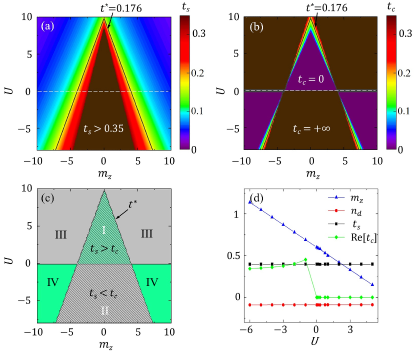
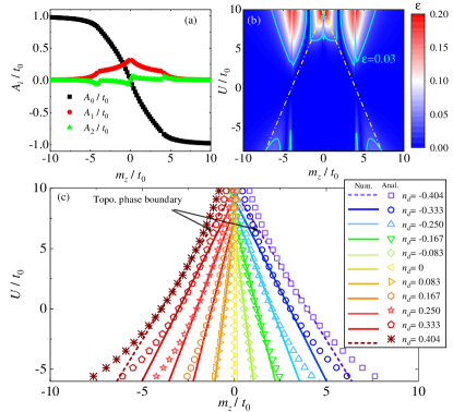
with , , , and , where corresponds to the sign of . We clearly observe that is associated with and . Since the contour lines of have the linear form of interaction strength and Zeeman coupling , this characteristic time also has a similar linear scaling for a fixed , which is presented in Fig. 3(a) and fully matches with the numerical results.
IV.2 Dynamical topological phase transition and characteristic time
We now theoretically determine the characteristic time from the dynamical topological phase transition of post-quenched Hamiltonian . As we known, the dynamical topological phase transition is a phase transition in time driven by sharp internal changes in the properties of a quantum many-body state and not driven by an external control parameter [76, 77]. Quantum quenching is one way to induce the dynamical phase transitions. When we performing the quench dynamics for this system, the value of generally decays with the time evolution and approaches steady since the initial state is prepared into a nearly fully polarized state for and has . When the interaction strength satisfies , we find that the time-dependent effective Zeeman coupling only passes through one phase transition point, i.e., for or for . Moreover, the corresponding crossover may occurs multiple times. Hence only changes from the trivial (topological) regime at to the topological (trivial) regime for , when the interaction is repulsive (attractive). To describe the critical time of the dynamical topological phase transition, the characteristic time is naturally defined as
| (14) |
We have and ( and ) in the repulsive (attractive) interaction regime when and respectively. Here of the repulsive interaction means that the topology of is always trivial in a long evolved time, while a finite implies that its topology is changed from the trivial case with to the topological case with .
With the precise definition of , we next numerically show it in Fig. 2, where only passes though the phase transition point and decays (increases) for the repulsive (attractive) interaction in the short time region. Note that this feature can be described by the analytical in Appendix B, where we have for due to . Besides, we should choose the minimum time scale in the Eq. (14) which is similar to , since the instantaneous state is not self-consistent and there may be multiple time points to satisfy this requirement.
Like Eq. (13), we also obtain an analytical result for in the short-time evolution [see Appendix B] as follows:
| (15) |
with , , and . Compared with , the characteristic time presents a completely different scaling form in terms of the Zeeman coupling and interaction strength, expect for the topological phase boundaries [see Fig. 3(b)]. This also implies that happens on these topological boundaries. On the other hand, we observe that the finite only appears around the topological phase boundaries. The reason is that always remains topological or trivial case when it is far away from the phase boundaries [This also causes the unchanged dynamical invariant of Eq. (22) in the evolution], as we show in Figs. 5(b) and 5(d).
IV.3 Characteristic time and its linear scaling
We now theoretically determine the characteristic time . Since the post-quenched parameters on the topological phase boundaries keep , a special evolution time can be defined on these topological phase boundaries by
| (16) |
which holds the nontrivial relation [see Figs. 3(a) and 3(b)]. This point can be clearly observed by taking in the Eqs. (13) and (15), which synchronously gives
| (17) |
where , , and ; see Appendix B. For the parameters on the topological boundaries, the gap closing occurs at Dirac points or , which is naturally captured by . Besides, it should be noted that is only a time scale corresponding to these topological boundaries and has slightly difference with the previous and which can cover all parameters. In particular, we see that the analytical is associated with and , where is usually a constant in the topological phase boundaries and has the linear scaling for the Zeeman coupling and interaction. Hence shall inherit these linear properties and only depend on the spin-orbit coupled strength. As it is shown in Fig. 3, we have for a strong spin-orbit coupling with , which theoretically gives when and this matches with the numerical result [see Fig. 5(b)].
V Mean-field phase diagram determined by time scales
In this section, we establish the dynamical characterization via the above three time scales. Further, we accurately determine the Chern number by examining the spin dynamics at four Dirac points. Particularly, we demonstrate the correctness of mean-field phase diagram by comparing the dynamical measurement results with the theoretical self-consistent results.
V.1 Dynamical characterization
In the previous quench dynamics, this interacting system shall emerge the different time scales in the different post-quenched topological phases with the repulsive (attractive) interaction, when is trivial (topological) at . Specifically, the relations of three time scales are given via the four regimes of Fig. 3(c). Regime I (, topological phase): , , and ; Regime II (, topological phase): , , and ; Regime III (, trivial phase): , , and ; Regime IV (, trivial phase): , , and . Equivalently, the correspondence between the characteristic times and the equilibrium topological properties is given by
| (18) |
The formula provides a convenient dynamical way to determine the mean-field topological phase by comparing any two characteristic time scales. Moreover, both the numerical results [Fig. 2] and the analytical results [Fig. 3(c)] confirm this way, especially for weak interaction or small , as we show in Fig. 3(d). Hence we only need to prepare an initial nearly fully polarized state and perform quenching, and then the mean-field topological phases can be directly determined by comparing any two time scales.
V.2 Determination of Chern number
For the equilibrium mean-field topological phases of Eq. (18), we further need to accurately determine the Chern number by considering the features of spin dynamics. Specifically, the time-dependent spin evolution of this interacting system is described by the modified Landau-Lifshitz equation [123]
| (19) |
with
| (20) |
The topological number of the time-dependent post-quenched Hamiltonian is determined by the spin dynamics of at four Dirac points . The Chern number of the equilibrium mean-field Hamiltonian is then obtained by .
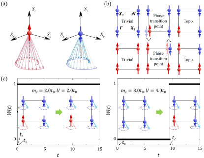
We next show two fundamental spin dynamical properties of this interacting system. Firstly, the spin at four Dirac points of the nearly fully polarized initial state will move around the corresponding polarization direction of after the quantum quench. When the polarization direction is reversed, e.g., from upward to downward, the motion of spin will be reversed at the same time, e.g., from clockwise to counterclockwise; see Fig. 4(a). For this, we can use the motion of spins to determine the polarization direction of at Dirac points. Second, since the polarization direction is associated with the parity eigenvalue of the occupied eigenstate, the topology of can be identified from the polarization directions at four Dirac points [68], as shown in Fig. 4(b). For instance, the polarization directions at four Dirac points are the same for an initial trivial Hamiltonian . Once it enters the topological regime, the motion of spin at or point will be reversed, manifesting the change of the corresponding polarization direction. This signal can be captured by , as shown in Fig. 5(d). Correspondingly, the topological transition time of the motion of spin just gives the characteristic time .
With above two fundamental properties, we can define the time-dependent dynamical invariant for as
| (21) |
with for the topological regime and for the trivial regime , respectively. The topological transition time of this dynamical invariant gives the characteristic time as follows:
| (22) |
Here a finite is captured by the critical time of changing of from () to () [see Figs. 3(b) and 5(d)], while the unchanged in a long-time evolution hosts or . Now the topological number of and the Chern number of can be exactly given by
| (23) |
As an example, the numerical results in Fig. 4(c) show the nontrivial topology with and the trivial topology with for the post-quenched system with and , respectively. On the other hand, since there is only one topological phase transition point in the dynamical evolution, has the same value at with . Hence we also have
| (24) |
It should be emphasized that any one formula of the Eqs. (23) and (24) facilitates the determination of Chern number of the equilibrium mean-field topological phases for the post-quenched system. In the following, we take Eq. (24) in the experiment for identifying the Chern number due to the easy measurement of .
VI Experimental detection
Based on above topological characterization, we next propose a feasible experimental scheme to detect the mean-field topological phase diagram by directly measuring the two characteristic time scales and , without any prior post-quenched parameters such as and . Note that the measurement of is almost impossible in the recent experiment, since it does not have any measurable quantities but only corresponds to the self-consistency of post-quenched Hamiltonian.
In a realistic experiment, identifying the time scale of needs to measure the spin dynamics of at four Dirac points in a short-time evolution and calculate their changing with the evolved time, i.e., . And then, is captured by the topological transition time of based on the Eq. (22). On the other hand, we need to measure the time-dependent particle density and calculate the fastest changing of with the evolved time and identify the time scale of by an auxiliary time
| (25) |
We see that characterizes the evolution of changes fastestly, i.e., is maximal. Particularly, occurs on the topological phase boundaries although it is larger (smaller) than in the topological (trivial) regime [see Fig. 5(c)]. This point can be clearly observed by an analytical result from Eq. (25), i.e.,
| (26) |
with and . This formula is consistent with Eq. (17). Also, we have for , which is approximately equal to in the Eq. (17).
With above observation, the mean-field topological phase diagram can be obtained by only comparing both time scales of and ; see Fig. 5(a). Considering that the 2D QAH model has realized in the cold atoms [60] and the interaction can be can be tuned in experiment [43], we hereby provide the following four concrete steps to detect the equilibrium mean-field topological phases for the cold atom experiment:
-
Step I: preparing the nearly fully polarized initial state for the system with , which can be reached by tuning say magnetic field for ultracold atoms. By further varying the two-photon detuning via the bias magnetic field to produce a large , together with turning off one of the electro-optic modulators to generate the small constant magnetization or [124], the nearly fully polarized state is now obtained;
-
Step II: performing quench dynamics for this system with . We suddenly change the magnetic field to produce a finite and turn off both the electro-optic modulators to generate , which drives the system evolve with the time. And then, we measure the time-dependent particle density . The time scale of is obtained by the fastest changing time point of . Note that this has the linear scaling on the mean-field topological phase boundaries [see Fig. 3(c)] and is independent of . Hence can be directly employed to the cases of ;
-
Step III: preparing the nearly fully polarized initial state for the system with . This step is similar to Step I. Here can be an unknown value;
-
Step IV: performing quench dynamics for this system with the nonzero . For this we suddenly tune the system to a regime with an unknown suitable and turn off both the electro-optic modulators to generate . Simultaneously, we measure the evolution of at four Dirac points and obtain their changing with the evolved time, i.e., . Then is captured by the topological transition time of based on the Eq. (22). Finally, the mean-field topological phases are identified by comparing in the Step II and in the Step IV, where the Chern number is given by ; see Eq. (24).
With this scheme, the mean-field phase diagram of the interacting Chern insulator can be completely determined, which paves the way to experimentally study topological phases in interacting systems and discover new phases.
VII Conclusion and discussion
In conclusion, we have studied the 2D QAH model with a weak-to-intermediate Hubbard interaction by performing quantum quenches. A nonequilibrium detection scheme for the mean-field topological phase diagram is proposed by observing three characteristic times , , and emerged in dynamics. We reveals three nontrivial dynamical properties: (i) and capture the emergence of dynamical self-consistent particle density and dynamical topological phase transition for the time-dependent post-quenched Hamiltonian respectively, while gives a linear scaling time on the topological phase boundaries; (ii) After quenching the Zeeman coupling from the trivial regime to the topological regime, () is observed for the repulsive (attractive) interaction; (iii) The Chern number of post-quenched mean-field topological phase can be determined by comparing any two time scales. These results provide a feasible scheme to detect the mean-field topological phases of an interacting Chern insulator and may be applied to the quantum simulation experiments.
The present dynamical scheme can be applied to the Chern insulator with the weak-to-intermediate interaction. On the other hand, when the general strong interactions are considered, the system may host more abundant magnetic phases [115, 116, 117]. Generalizing these dynamical properties to the related studies and further identifying the rich topological phases would be an interesting and worthwhile work in the future.
ACKNOWLEDGEMENT
We acknowledge the valuable discussions with Sen Niu and Ting Fung Jeffrey Poon. This work was supported by National Natural Science Foundation of China (Grants No. 11825401 and No. 11921005), the National Key R&D Program of China (Project No. 2021YFA1400900), Strategic Priority Research Program of the Chinese Academy of Science (Grant No. XDB28000000), and by the Open Project of Shenzhen Institute of Quantum Science and Engineering (Grant No.SIQSE202003). Long Zhang also acknowledges support from the startup grant of the Huazhong University of Science and Technology (Grant No. 3004012191). Lin Zhang also acknowledges support from Agencia Estatal de Investigación (the R&D project CEX2019-000910-S, funded by MCIN/AEI/10.13039/501100011033, Plan National FIDEUA PID2019-106901GB-I00, FPI), Fundació Privada Cellex, Fundació Mir-Puig, Generalitat de Catalunya (AGAUR Grant No. 2017 SGR 1341, CERCA program), EU Horizon 2020 FET-OPEN OPTOlogic (Grant No. 899794), and Junior Leaders fellowship LCF/BQ/PI19/11690013 of ”La Caixa” Foundation (ID100010434).
Appendix A Equilibrium analytical results
In presence of the non-zero interaction, the equilibrium mean-field Hamiltonian self-consistently gives the difference of density for spin-up and spin-down particles as under the mean field theory. Here we explicitly show
| (27) |
Considering that is a small value due to the total particle density is conserved, i.e., , we use Taylor series at for the right-hand term of Eq. (27), which gives with th-order truncation . Here the coefficients satisfy . In principle, we can obtain by solving . The analytical for at a weak interaction or a small Zeeman coupling is approximately given by
| (28) |
with , , and . The Eq. (28) shows the scaling property of for and .
Besides, we observe that can converge to zero for an increased ; see Fig. 6(a). For a 3rd-order truncation in Eq. (28), the absolute error between analytical and numerical results presents for , which implies that the precision of 3rd-order truncation is enough. Therefore, this Eq. (28) is applicable to the almost completely topological phase region and all the topological phase boundaries and a large trivial regions, as shown in Fig. 6(b). Also, the analytical results are almost confirmed with the numerical results for both a weak interaction or a small , as shown in Fig. 6(c).
Appendix B Nonequilibrium analytical results
Considering that the spin of initial state is nearly fully polarized to downward or upward, we can take or , which corresponds to the post-quenched or . Further, the change of is small during a short-time evolution and it can be regarded as a constant in a very short time. By solving Eq. (4), we can obtain and which is given by
| (29) |
where and corresponds to the sign of the post-quenched . Similarly, we use Taylor series at for the right-hand term of Eq. (29), which gives with th-order truncation .
We next take the 3rd-order truncation to approximately obtain as follows:
| (30) |
with , , and . Note that here we have used Taylor series at for and have taken 6th-order truncation for ,. Then this approximate is only suitable for a short-time evolution or a small value of . Finally, we explicitly give , , , and by solving the equations of , , , and respectively, where the theoretical results are shown in Eq. (13), Eq. (15), Eq. (17), and Eq. (26).
Appendix C Dynamical self-consistent processes of particle density
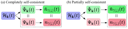
There are two cases of the dynamical self-consistent processes to obtain the self-consistent particle density . The first one is a completely self-consistent process. Namely, both wave function and particle density are self-consistently, as it is shown in Fig. 7(a). By diagonalizing the time-dependent Hamiltonian and obtaining its eigenvector with negative energy. Next the instantaneous wave function should equal to at each momentum , i.e., . It is clear that the self-consistent wave function directly gives from the Eq. (5) and Eq. (11). Particularly, we emphasize that this system shall reach a dynamical balance and both and do not evolve with the time, when becomes the eigenvector of .
The second one is a partially self-consistent process. Namely, only particle density is self-consistently, as it is shown in Fig. 7(b). After obtaining the eigenvector with negative energy of , the difference with the above process is to directly take this equal , of which we do not care the instantaneous states. It is clear that the self-consistent particle density are also given by , but now the wave function is not self-consistent, i.e., . Physically, the particle density is associated with the summation of the wave function at all , which implies that the wave function of each may not be self-consistent but the summation for all can be self-consistent.
Both two processes can give the self-consistent particle density of post-quenched Hamiltonian , while the former is difficult to realize the completely self-consistent in a long-term evolution. The latter is easily obtained in a short-time evolution and is more helpful to capture the nontrivial dynamics.
References
- v. Klitzing et al. [1980] K. v. Klitzing, G. Dorda, and M. Pepper, New method for high-accuracy determination of the fine-structure constant based on quantized Hall resistance, Phys. Rev. Lett. 45, 494 (1980).
- Tsui et al. [1982] D. C. Tsui, H. L. Stormer, and A. C. Gossard, Two-dimensional magnetotransport in the extreme quantum limit, Phys. Rev. Lett. 48, 1559 (1982).
- Hasan and Kane [2010] M. Z. Hasan and C. L. Kane, Colloquium: topological insulators, Rev. Mod. Phys. 82, 3045 (2010).
- Wen [2017] X.-G. Wen, Colloquium: Zoo of quantum-topological phases of matter, Rev. Mod. Phys. 89, 041004 (2017).
- Kosterlitz [2017] J. M. Kosterlitz, Nobel lecture: topological defects and phase transitions, Rev. Mod. Phys. 89, 040501 (2017).
- Wen [1990] X.-G. Wen, Topological orders in rigid states, Int. J. of Mod. Phys. B 4, 239 (1990).
- Qi and Zhang [2011] X.-L. Qi and S.-C. Zhang, Topological insulators and superconductors, Rev. Mod. Phys. 83, 1057 (2011).
- Fu et al. [2007] L. Fu, C. L. Kane, and E. J. Mele, Topological insulators in three dimensions, Phys. Rev. Lett. 98, 106803 (2007).
- Fu and Kane [2007] L. Fu and C. L. Kane, Topological insulators with inversion symmetry, Phys. Rev. B 76, 045302 (2007).
- Fu [2011] L. Fu, Topological crystalline insulators, Phys. Rev. Lett. 106, 106802 (2011).
- Chang et al. [2013] C.-Z. Chang, J. Zhang, X. Feng, J. Shen, Z. Zhang, M. Guo, K. Li, Y. Ou, P. Wei, L.-L. Wang, Z.-Q. Ji, Y. Feng, S. Ji, X. Chen, J. Jia, X. Dai, Z. Fang, S.-C. Zhang, K. He, Y. Wang, L. Lu, X.-C. Ma, and Q.-K. Xue, Experimental observation of the quantum anomalous Hall effect in a magnetic topological insulator, Science 340, 167 (2013).
- Burkov and Balents [2011] A. A. Burkov and L. Balents, Weyl semimetal in a topological insulator multilayer, Phys. Rev. Lett. 107, 127205 (2011).
- Young et al. [2012] S. M. Young, S. Zaheer, J. C. Y. Teo, C. L. Kane, E. J. Mele, and A. M. Rappe, Dirac semimetal in three dimensions, Phys. Rev. Lett. 108, 140405 (2012).
- Xu et al. [2015] S.-Y. Xu, I. Belopolski, N. Alidoust, M. Neupane, G. Bian, C. Zhang, R. Sankar, G. Chang, Z. Yuan, C.-C. Lee, S.-M. Huang, H. Zheng, J. Ma, D. S. Sanchez, B. Wang, A. Bansil, F. Chou, P. P. Shibayev, H. Lin, S. Jia, and M. Z. Hasan, Discovery of a Weyl fermion semimetal and topological Fermi arcs, Science 349, 613 (2015).
- Lv et al. [2015] B. Q. Lv, H. M. Weng, B. B. Fu, X. P. Wang, H. Miao, J. Ma, P. Richard, X. C. Huang, L. X. Zhao, G. F. Chen, Z. Fang, X. Dai, T. Qian, and H. Ding, Experimental discovery of Weyl semimetal TaAs, Phys. Rev. X 5, 031013 (2015).
- Qi et al. [2009] X.-L. Qi, T. L. Hughes, S. Raghu, and S.-C. Zhang, Time-reversal-invariant topological superconductors and superfluids in two and three dimensions, Phys. Rev. Lett. 102, 187001 (2009).
- Bernevig and Hughes [2013] B. A. Bernevig and T. L. Hughes, Topological insulators and topological superconductors (Princeton university press, 2013).
- Ando and Fu [2015] Y. Ando and L. Fu, Topological crystalline insulators and topological superconductors: From concepts to materials, Annu. Rev. Condens. Matter Phys. 6, 361 (2015).
- Sato and Ando [2017] M. Sato and Y. Ando, Topological superconductors: a review, Rep. Prog. Phys. 80, 076501 (2017).
- Zhang et al. [2018a] P. Zhang, K. Yaji, T. Hashimoto, Y. Ota, T. Kondo, K. Okazaki, Z. Wang, J. Wen, G. Gu, H. Ding, and S. Shin, Observation of topological superconductivity on the surface of an iron-based superconductor, Science 360, 182 (2018a).
- Wang et al. [2010] Z. Wang, X.-L. Qi, and S.-C. Zhang, Topological order parameters for interacting topological insulators, Phys. Rev. Lett. 105, 256803 (2010).
- Pesin and Balents [2010] D. Pesin and L. Balents, Mott physics and band topology in materials with strong spin–orbit interaction, Nat. Phys. 6, 376 (2010).
- Lee [2011] D.-H. Lee, Effects of interaction on quantum spin Hall insulators, Phys. Rev. Lett. 107, 166806 (2011).
- Castro et al. [2011] E. V. Castro, A. G. Grushin, B. Valenzuela, M. A. H. Vozmediano, A. Cortijo, and F. de Juan, Topological fermi liquids from coulomb interactions in the doped honeycomb lattice, Phys. Rev. Lett. 107, 106402 (2011).
- Araújo et al. [2013] M. A. N. Araújo, E. V. Castro, and P. D. Sacramento, Change of an insulator’s topological properties by a Hubbard interaction, Phys. Rev. B 87, 085109 (2013).
- Yao and Ryu [2013] H. Yao and S. Ryu, Interaction effect on topological classification of superconductors in two dimensions, Phys. Rev. B 88, 064507 (2013).
- Messer et al. [2015] M. Messer, R. Desbuquois, T. Uehlinger, G. Jotzu, S. Huber, D. Greif, and T. Esslinger, Exploring competing density order in the ionic Hubbard model with ultracold fermions, Phys. Rev. Lett. 115, 115303 (2015).
- Spanton et al. [2018] E. M. Spanton, A. A. Zibrov, H. Zhou, T. Taniguchi, K. Watanabe, M. P. Zaletel, and A. F. Young, Observation of fractional chern insulators in a van der waals heterostructure, Science 360, 62 (2018).
- Rachel [2018] S. Rachel, Interacting topological insulators: a review, Rep. Prog. Phys. 81, 116501 (2018).
- Viyuela et al. [2018] O. Viyuela, L. Fu, and M. A. Martin-Delgado, Chiral topological superconductors enhanced by long-range interactions, Phys. Rev. Lett. 120, 017001 (2018).
- Andrews and Soluyanov [2020] B. Andrews and A. Soluyanov, Fractional quantum hall states for moiré superstructures in the hofstadter regime, Phys. Rev. B 101, 235312 (2020).
- Mook et al. [2021] A. Mook, K. Plekhanov, J. Klinovaja, and D. Loss, Interaction-stabilized topological magnon insulator in ferromagnets, Phys. Rev. X 11, 021061 (2021).
- Raghu et al. [2008] S. Raghu, X.-L. Qi, C. Honerkamp, and S.-C. Zhang, Topological Mott Insulators, Phys. Rev. Lett. 100, 156401 (2008).
- Rachel and Le Hur [2010] S. Rachel and K. Le Hur, Topological insulators and Mott physics from the Hubbard interaction, Phys. Rev. B 82, 075106 (2010).
- Vanhala et al. [2016] T. I. Vanhala, T. Siro, L. Liang, M. Troyer, A. Harju, and P. Törmä, Topological phase transitions in the repulsively interacting Haldane-Hubbard model, Phys. Rev. Lett. 116, 225305 (2016).
- Qi et al. [2006] X.-L. Qi, Y.-S. Wu, and S.-C. Zhang, Topological quantization of the spin hall effect in two-dimensional paramagnetic semiconductors, Phys. Rev. B 74, 085308 (2006).
- Qi et al. [2010] X.-L. Qi, T. L. Hughes, and S.-C. Zhang, Chiral topological superconductor from the quantum Hall state, Phys. Rev. B 82, 184516 (2010).
- Liu et al. [2014] X.-J. Liu, K. T. Law, and T. K. Ng, Realization of 2D spin-orbit interaction and exotic topological orders in cold atoms, Phys. Rev. Lett. 112, 086401 (2014).
- Ting Fung Jeffrey Poon and Liu [2018] Ting Fung Jeffrey Poon and X.-J. Liu, From a semimetal to a chiral Fulde-Ferrell superfluid, Phys. Rev. B 97, 020501(R) (2018).
- Hofstetter and Qin [2018] W. Hofstetter and T. Qin, Quantum simulation of strongly correlated condensed matter systems, J. Phys. B 51, 082001 (2018).
- Fauseweh and Zhu [2021] B. Fauseweh and J.-X. Zhu, Digital quantum simulation of non-equilibrium quantum many-body systems, Quant. Info. Proc. 20, 138 (2021).
- Monroe et al. [2021] C. Monroe, W. C. Campbell, L.-M. Duan, Z.-X. Gong, A. V. Gorshkov, P. W. Hess, R. Islam, K. Kim, N. M. Linke, G. Pagano, P. Richerme, C. Senko, and N. Y. Yao, Programmable quantum simulations of spin systems with trapped ions, Rev. Mod. Phys. 93, 025001 (2021).
- Bloch et al. [2008] I. Bloch, J. Dalibard, and W. Zwerger, Many-body physics with ultracold gases, Rev. Mod. Phys. 80, 885 (2008).
- Langen et al. [2015] T. Langen, R. Geiger, and J. Schmiedmayer, Ultracold atoms out of equilibrium, Annu. Rev. Condens. Matter Phys. 6, 201 (2015).
- Gross and Bloch [2017] C. Gross and I. Bloch, Quantum simulations with ultracold atoms in optical lattices, Science 357, 995 (2017).
- Schreiber et al. [2015] M. Schreiber, S. S. Hodgman, P. Bordia, H. P. Lüschen, M. H. Fischer, R. Vosk, E. Altman, U. Schneider, and I. Bloch, Observation of many-body localization of interacting fermions in a quasirandom optical lattice, Science 349, 842 (2015).
- Smith et al. [2016] J. Smith, A. Lee, P. Richerme, B. Neyenhuis, P. W. Hess, P. Hauke, M. Heyl, D. A. Huse, and C. Monroe, Many-body localization in a quantum simulator with programmable random disorder, Nat. Phys. 12, 907 (2016).
- Bordia et al. [2016] P. Bordia, H. P. Lüschen, S. S. Hodgman, M. Schreiber, I. Bloch, and U. Schneider, Coupling identical one-dimensional many-body localized systems, Phys. Rev. Lett. 116, 140401 (2016).
- Choi et al. [2016] J.-y. Choi, S. Hild, J. Zeiher, P. Schauß, A. Rubio-Abadal, T. Yefsah, V. Khemani, D. A. Huse, I. Bloch, and C. Gross, Exploring the many-body localization transition in two dimensions, Science 352, 1547 (2016).
- Ramasesh et al. [2017] V. V. Ramasesh, E. Flurin, M. Rudner, I. Siddiqi, and N. Y. Yao, Direct probe of topological invariants using Bloch oscillating quantum walks, Phys. Rev. Lett. 118, 130501 (2017).
- Jiang et al. [2018] Z. Jiang, K. J. Sung, K. Kechedzhi, V. N. Smelyanskiy, and S. Boixo, Quantum algorithms to simulate many-body physics of correlated fermions, Phys. Rev. Applied 9, 044036 (2018).
- Yan et al. [2019] Z. Yan, Y.-R. Zhang, M. Gong, Y. Wu, Y. Zheng, S. Li, C. Wang, F. Liang, J. Lin, Y. Xu, C. Guo, L. Sun, C.-Z. Peng, K. Xia, H. Deng, H. Rong, J. Q. You, F. Nori, H. Fan, X. Zhu, and J.-W. Pan, Strongly correlated quantum walks with a 12-qubit superconducting processor, Science 364, 753 (2019).
- Su et al. [1980] W. P. Su, J. R. Schrieffer, and A. J. Heeger, Soliton excitations in polyacetylene, Phys. Rev. B 22, 2099 (1980).
- Atala et al. [2013] M. Atala, M. Aidelsburger, J. T. Barreiro, D. Abanin, T. Kitagawa, E. Demler, and I. Bloch, Direct measurement of the Zak phase in topological Bloch bands, Nat. Phys. 9, 795 (2013).
- Liu et al. [2013a] X.-J. Liu, Z.-X. Liu, and M. Cheng, Manipulating topological edge spins in a one-dimensional optical lattice, Phys. Rev. Lett. 110, 076401 (2013a).
- Song et al. [2018] B. Song, L. Zhang, C. He, T. F. J. Poon, E. Hajiyev, S. Zhang, X.-J. Liu, and G.-B. Jo, Observation of symmetry-protected topological band with ultracold fermions, Sci. Adv. 4, eaao4748 (2018).
- Haldane [1983] F. D. M. Haldane, Continuum dynamics of the 1-D Heisenberg antiferromagnet: Identification with the O (3) nonlinear sigma model, Phys. Lett. A 93, 464 (1983).
- de Léséleuc et al. [2019] S. de Léséleuc, V. Lienhard, P. Scholl, D. Barredo, S. Weber, N. Lang, H. P. Büchler, T. Lahaye, and A. Browaeys, Observation of a symmetry-protected topological phase of interacting bosons with Rydberg atoms, Science 365, 775 (2019).
- Jotzu et al. [2014] G. Jotzu, M. Messer, R. Desbuquois, M. Lebrat, T. Uehlinger, D. Greif, and T. Esslinger, Experimental realization of the topological Haldane model with ultracold fermions, Nature 515, 237 (2014).
- Wu et al. [2016] Z. Wu, L. Zhang, W. Sun, X.-T. Xu, B.-Z. Wang, S.-C. Ji, Y. Deng, S. Chen, X.-J. Liu, and J.-W. Pan, Realization of two-dimensional spin-orbit coupling for Bose-Einstein condensates, Science 354, 83 (2016).
- Sun et al. [2018a] W. Sun, B.-Z. Wang, X.-T. Xu, C.-R. Yi, L. Zhang, Z. Wu, Y. Deng, X.-J. Liu, S. Chen, and J.-W. Pan, Highly controllable and robust 2D spin-orbit coupling for quantum gases, Phys. Rev. Lett. 121, 150401 (2018a).
- Liang et al. [2023] M.-C. Liang, Y.-D. Wei, L. Zhang, X.-J. Wang, H. Zhang, W.-W. Wang, W. Qi, X.-J. Liu, and X. Zhang, Realization of qi-wu-zhang model in spin-orbit-coupled ultracold fermions, Phys. Rev. Research 5, L012006 (2023).
- He et al. [2016] W.-Y. He, S. Zhang, and K. T. Law, Realization and detection of Weyl semimetals and the chiral anomaly in cold atomic systems, Phys. Rev. A 94, 013606 (2016).
- Wang et al. [2018] B.-Z. Wang, Y.-H. Lu, W. Sun, S. Chen, Y. Deng, and X.-J. Liu, Dirac-, rashba-, and weyl-type spin-orbit couplings: Toward experimental realization in ultracold atoms, Phys. Rev. A 97, 011605(R) (2018).
- Lu et al. [2020] Y.-H. Lu, B.-Z. Wang, and X.-J. Liu, Ideal weyl semimetal with 3d spin-orbit coupled ultracold quantum gas, Sci. Bull. 65, 2080 (2020).
- Wang et al. [2021] Z.-Y. Wang, X.-C. Cheng, B.-Z. Wang, J.-Y. Zhang, Y.-H. Lu, C.-R. Yi, S. Niu, Y. Deng, X.-J. Liu, S. Chen, and J.-W. Pan, Realization of an ideal Weyl semimetal band in a quantum gas with 3D spin-orbit coupling, Science 372, 271 (2021).
- Li and Liu [2021] X. Li and W. V. Liu, Weyl semimetal made ideal with a crystal of raman light and atoms, Sci. Bull. 66, 1253 (2021).
- Liu et al. [2013b] X.-J. Liu, K.-T. Law, T.-K. Ng, and P. A. Lee, Detecting topological phases in cold atoms, Phys. Rev. Lett. 111, 120402 (2013b).
- Hafezi [2014] M. Hafezi, Measuring topological invariants in photonic systems, Phys. Rev. Lett. 112, 210405 (2014).
- Wu et al. [2014] J. Wu, J. Liu, and X.-J. Liu, Topological spin texture in a quantum anomalous Hall insulator, Phys. Rev. Lett. 113, 136403 (2014).
- Price et al. [2016] H. M. Price, O. Zilberberg, T. Ozawa, I. Carusotto, and N. Goldman, Measurement of Chern numbers through center-of-mass responses, Phys. Rev. B 93, 245113 (2016).
- Vajna and Dóra [2015] S. Vajna and B. Dóra, Topological classification of dynamical phase transitions, Phys. Rev. B 91, 155127 (2015).
- Hu et al. [2016] Y. Hu, P. Zoller, and J. C. Budich, Dynamical buildup of a quantized hall response from nontopological states, Phys. Rev. Lett. 117, 126803 (2016).
- Budich and Heyl [2016] J. C. Budich and M. Heyl, Dynamical topological order parameters far from equilibrium, Phys. Rev. B 93, 085416 (2016).
- Wilson et al. [2016] J. H. Wilson, J. C. W. Song, and G. Refael, Remnant geometric Hall response in a quantum quench, Phys. Rev. Lett. 117, 235302 (2016).
- Heyl [2018] M. Heyl, Dynamical quantum phase transitions: a review, Rep. Prog. Phys. 81, 054001 (2018).
- Heyl [2019] M. Heyl, Dynamical quantum phase transitions: a brief survey, EPL 125, 26001 (2019).
- Hu et al. [2020] H. Hu, B. Huang, E. Zhao, and W. V. Liu, Dynamical singularities of floquet higher-order topological insulators, Phys. Rev. Lett. 124, 057001 (2020).
- Hu and Zhao [2020] H. Hu and E. Zhao, Topological invariants for quantum quench dynamics from unitary evolution, Phys. Rev. Lett. 124, 160402 (2020).
- Kuo et al. [2021] W.-T. Kuo, D. Arovas, S. Vishveshwara, and Y.-Z. You, Decoherent quench dynamics across quantum phase transitions, SciPost Phys. 11, 084 (2021).
- Cai and Yi [2022] D.-H. Cai and W. Yi, Synthetic topology and floquet dynamic quantum phase transition in a periodically driven raman lattice, Phys. Rev. A 105, 042812 (2022).
- Zhang et al. [2018b] L. Zhang, L. Zhang, S. Niu, and X.-J. Liu, Dynamical classification of topological quantum phases, Sci. Bull. 63, 1385 (2018b).
- Zhang et al. [2019a] L. Zhang, L. Zhang, and X.-J. Liu, Characterizing topological phases by quantum quenches: A general theory, Phys. Rev. A 100, 063624 (2019a).
- Ye and Li [2020] J. Ye and F. Li, Emergent topology under slow nonadiabatic quantum dynamics, Phys. Rev. A 102, 042209 (2020).
- Jia et al. [2021] W. Jia, L. Zhang, L. Zhang, and X.-J. Liu, Dynamically characterizing topological phases by high-order topological charges, Phys. Rev. A 103, 052213 (2021).
- Li et al. [2021] L. Li, W. Zhu, and J. Gong, Direct dynamical characterization of higher-order topological phases with nested band inversion surfaces, Sci. Bull. 66, 1502 (2021).
- Zhang et al. [2022a] L. Zhang, W. Jia, and X.-J. Liu, Universal topological quench dynamics for topological phases, Sci. Bull. 67, 1236 (2022a).
- Fang et al. [2022] P. Fang, Y.-X. Wang, and F. Li, Generic theory of characterizing topological phases under quantum slow dynamics, Phys. Rev. A 106, 022219 (2022).
- Sun et al. [2018b] W. Sun, C.-R. Yi, B.-Z. Wang, W.-W. Zhang, B. C. Sanders, X.-T. Xu, Z.-Y. Wang, J. Schmiedmayer, Y. Deng, X.-J. Liu, S. Chen, and J.-W. Pan, Uncover topology by quantum quench dynamics, Phys. Rev. Lett. 121, 250403 (2018b).
- Tarnowski et al. [2019] M. Tarnowski, F. N. Ünal, N. Fläschner, B. S. Rem, A. Eckardt, K. Sengstock, and C. Weitenberg, Measuring topology from dynamics by obtaining the Chern number from a linking number, Nat. Commun. 10, 1728 (2019).
- Yi et al. [2019] C.-R. Yi, L. Zhang, L. Zhang, R.-H. Jiao, X.-C. Cheng, Z.-Y. Wang, X.-T. Xu, W. Sun, X.-J. Liu, S. Chen, and J.-W. Pan, Observing topological charges and dynamical bulk-surface correspondence with ultracold atoms, Phys. Rev. Lett. 123, 190603 (2019).
- Wang et al. [2019] Y. Wang, W. Ji, Z. Chai, Y. Guo, M. Wang, X. Ye, P. Yu, L. Zhang, X. Qin, P. Wang, F. Shi, X. Rong, D. Lu, X.-J. Liu, and J. Du, Experimental observation of dynamical bulk-surface correspondence in momentum space for topological phases, Phys. Rev. A 100, 052328 (2019).
- Xin et al. [2020] T. Xin, Y. Li, Y.-a. Fan, X. Zhu, Y. Zhang, X. Nie, J. Li, Q. Liu, and D. Lu, Quantum Phases of Three-Dimensional Chiral Topological Insulators on a Spin Quantum Simulator, Phys. Rev. Lett. 125, 090502 (2020).
- Ji et al. [2020] W. Ji, L. Zhang, M. Wang, L. Zhang, Y. Guo, Z. Chai, X. Rong, F. Shi, X.-J. Liu, Y. Wang, and J. Du, Quantum simulation for three-dimensional chiral topological insulator, Phys. Rev. Lett. 125, 020504 (2020).
- Niu et al. [2021] J. Niu, T. Yan, Y. Zhou, Z. Tao, X. Li, W. Liu, L. Zhang, H. Jia, S. Liu, Z. Yan, Y. Chen, and D. Yu, Simulation of higher-order topological phases and related topological phase transitions in a superconducting qubit, Sci. Bull. 66, 1168 (2021).
- Chen et al. [2021] B. Chen, S. Li, X. Hou, F. Ge, F. Zhou, P. Qian, F. Mei, S. Jia, N. Xu, and H. Shen, Digital quantum simulation of floquet topological phases with a solid-state quantum simulator, Photonics Res. 9, 81 (2021).
- Yu et al. [2021] D. Yu, B. Peng, X. Chen, X.-J. Liu, and L. Yuan, Topological holographic quench dynamics in a synthetic frequency dimension, Light Sci. Appl. 10, 209 (2021).
- Zhang et al. [2022b] J.-H. Zhang, B.-B. Wang, F. Mei, J. Ma, L. Xiao, and S. Jia, Topological optical raman superlattices, Phys. Rev. A 105, 033310 (2022b).
- Manmana et al. [2007] S. R. Manmana, S. Wessel, R. M. Noack, and A. Muramatsu, Strongly correlated fermions after a quantum quench, Phys. Rev. Lett. 98, 210405 (2007).
- Polkovnikov et al. [2011] A. Polkovnikov, K. Sengupta, A. Silva, and M. Vengalattore, Colloquium: Nonequilibrium dynamics of closed interacting quantum systems, Rev. Mod. Phys. 83, 863 (2011).
- Kiendl and Marquardt [2017] T. Kiendl and F. Marquardt, Many-particle dephasing after a quench, Phys. Rev. Lett. 118, 130601 (2017).
- Zhang et al. [2021] L. Zhang, L. Zhang, Y. Hu, S. Niu, and X.-J. Liu, Nonequilibrium characterization of equilibrium correlated quantum phases, Phys. Rev. B 103, 224308 (2021).
- Moeckel and Kehrein [2008] M. Moeckel and S. Kehrein, Interaction quench in the Hubbard model, Phys. Rev. Lett. 100, 175702 (2008).
- Han and Sá de Melo [2012] L. Han and C. A. R. Sá de Melo, Evolution from BCS to BEC superfluidity in the presence of spin-orbit coupling, Phys. Rev. A 85, 011606(R) (2012).
- Foster et al. [2013] M. S. Foster, M. Dzero, V. Gurarie, and E. A. Yuzbashyan, Quantum quench in a superfluid: Winding numbers and topological states far from equilibrium, Phys. Rev. B 88, 104511 (2013).
- Dong et al. [2015] Y. Dong, L. Dong, M. Gong, and H. Pu, Dynamical phases in quenched spin–orbit-coupled degenerate fermi gas, Nat. Commun. 6, 1 (2015).
- Gornyi et al. [2005] I. V. Gornyi, A. D. Mirlin, and D. G. Polyakov, Interacting electrons in disordered wires: Anderson localization and low-T transport, Phys. Rev. Lett. 95, 206603 (2005).
- Eisert et al. [2015] J. Eisert, M. Friesdorf, and C. Gogolin, Quantum many-body systems out of equilibrium, Nat. Phys. 11, 124 (2015).
- Yao et al. [2017] N. Y. Yao, A. C. Potter, I.-D. Potirniche, and A. Vishwanath, Discrete time crystals: Rigidity, criticality, and realizations, Phys. Rev. Lett. 118, 030401 (2017).
- Peotta et al. [2021] S. Peotta, F. Brange, A. Deger, T. Ojanen, and C. Flindt, Determination of dynamical quantum phase transitions in strongly correlated many-body systems using loschmidt cumulants, Phys. Rev. X 11, 041018 (2021).
- Jia et al. [2019] W. Jia, Z.-H. Huang, X. Wei, Q. Zhao, and X.-J. Liu, Topological superfluids for spin-orbit coupled ultracold Fermi gases, Phys. Rev. B 99, 094520 (2019).
- Powell et al. [2022] P. D. Powell, G. Baym, and C. A. R. Sá de Melo, Superfluid transition temperature and fluctuation theory of spin-orbit-and Rabi-coupled fermions with tunable interactions, Phys. Rev. A 105, 063304 (2022).
- Esslinger [2010] T. Esslinger, Fermi-Hubbard physics with atoms in an optical lattice, Annu. Rev. Condens. Matter Phys. 1, 129 (2010).
- Tarruell and Sanchez-Palencia [2018] L. Tarruell and L. Sanchez-Palencia, Quantum simulation of the Hubbard model with ultracold fermions in optical lattices, C. R. Phys. 19, 365 (2018).
- Ziegler et al. [2022a] L. Ziegler, E. Tirrito, M. Lewenstein, S. Hands, and A. Bermudez, Correlated chern insulators in two-dimensional raman lattices: A cold-atom regularization of strongly coupled four-fermi field theories, Phys. Rev. Research 4, L042012 (2022a).
- Ziegler et al. [2022b] L. Ziegler, E. Tirrito, M. Lewenstein, S. Hands, and A. Bermudez, Large-N Chern insulators: Lattice field theory and quantum simulation approaches to correlation effects in the quantum anomalous Hall effect, Ann. Phys. 439, 168763 (2022b).
- Tirrito et al. [2022] E. Tirrito, S. Hands, and A. Bermudez, Large-S and tensor-network methods for strongly-interacting topological insulators, Symmetry 14, 799 (2022).
- Guo and Shen [2011] H. Guo and S.-Q. Shen, Topological phase in a one-dimensional interacting fermion system, Phys. Rev. B 84, 195107 (2011).
- Song et al. [2019] B. Song, C. He, S. Niu, L. Zhang, Z. Ren, X.-J. Liu, and G.-B. Jo, Observation of nodal-line semimetal with ultracold fermions in an optical lattice, Nat. Phys. 15, 911 (2019).
- Lin et al. [2011] Y.-J. Lin, K. Jiménez-García, and I. B. Spielman, Spin–orbit-coupled Bose–Einstein condensates, Nature 471, 83 (2011).
- Wang et al. [2012] P. Wang, Z.-Q. Yu, Z. Fu, J. Miao, L. Huang, S. Chai, H. Zhai, and J. Zhang, Spin-orbit coupled degenerate Fermi gases, Phys. Rev. Lett. 109, 095301 (2012).
- Williams et al. [2013] R. A. Williams, M. C. Beeler, L. J. LeBlanc, K. Jiménez-García, and I. B. Spielman, Raman-induced interactions in a single-component Fermi gas near an -wave Feshbach resonance, Phys. Rev. Lett. 111, 095301 (2013).
- Gilbert [2004] T. L. Gilbert, A phenomenological theory of damping in ferromagnetic materials, IEEE Trans. Magn. 40, 3443 (2004).
- Zhang et al. [2019b] L. Zhang, L. Zhang, and X.-J. Liu, Dynamical detection of topological charges, Phys. Rev. A 99, 053606 (2019b).