Object Type Clustering using Markov Directly-Follow Multigraph in Object-Centric Process Mining

Abstract

Object-centric process mining is a new paradigm with more realistic assumptions about underlying data by considering several case notions, e.g., an order handling process can be analyzed based on order, item, package, and route case notions. Including many case notions can result in a very complex model. To cope with such complexity, this paper introduces a new approach to cluster similar case notions based on Markov Directly-Follow Multigraph, which is an extended version of the well-known Directly-Follow Graph supported by many industrial and academic process mining tools. This graph is used to calculate a similarity matrix for discovering clusters of similar case notions based on a threshold. A threshold tuning algorithm is also defined to identify sets of different clusters that can be discovered based on different levels of similarity. Thus, the cluster discovery will not rely on merely analysts’ assumptions. The approach is implemented and released as a part of a python library, called processmining, and it is evaluated through a Purchase to Pay (P2P) object-centric event log file. Some discovered clusters are evaluated by discovering Directly Follow-Multigraph by flattening the log based on the clusters. The similarity between identified clusters is also evaluated by calculating the similarity between the behavior of the process models discovered for each case notion using inductive miner based on footprints conformance checking.

I Introduction

Recent studies challenge the idea of applying process mining based on only one case notion [17, 4, 19]. For example, a simple order handling process can have many potential case notions like order, item, package, and route, which enable analyzing the business process from different perspectives. Indeed, it is more realistic to consider an event to be related to several case notions as several business entities might get affected by performing an activity in a business process.

Object-Centric Event Log (OCEL) [7] is the standard for relating one event to multiple objects representing different case notions. Object-Centric Process Mining is a new paradigm in process mining supporting several case notions when analyzing such log files. These logs are considered to be closer to information systems’ data in reality [19]. There are a few studies that introduce process model discovery techniques from such log files, e.g., Directly-Follows Multigraph [17] and Object-Centric Petri nets [19].

Directly-Follows Multigraph (DFM) [17] is a graph that shows the relationship between activities in a business process by incorporating several case notions. Relations in DFM show how the control in the process can move from one activity to another based on a case notion. It can be considered as an equivalent graph like the well-known Directly-Follows Graph (DFG) but incorporates several case notions.

Figure 1 shows an example of a DFM discovered from a toy example log file containing 39 events related to four case notions, i.e., item, order, package, and route, where their corresponding flows are colored by red, dark-red, green, and dark-green, respectively. The model is discovered using PM4Py [5], which is a python library that supports process mining.

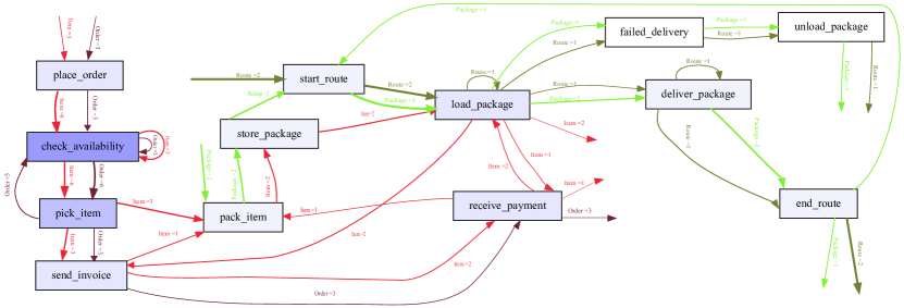
Figure 1: A Directly-Follows Multigraph (DFM), discovered from 39 events, indicates how process models incorporating all case notions can become complex.

As it can be seen in Figure 1, a DFM can easily become complex due to the existence of several case notions for each the process might have different underlying behavior. Separation of concerns is an approach to dealing with complexity in information systems [10, 12], which can be applied in this context by separating and classifying similar case notions into one category. Discovering process models with several case notions that share similar behavior can simplify the models and enable analyzing interesting aspects from OCEL.

Therefore, this paper introduces a new approach to cluster similar case notions based on Markov Directly-Follow Multigraph. This graph is used to calculate a similarity matrix which enables clustering of the case notions based on a threshold. A threshold tuning algorithm is also defined to identify sets of different clusters that can be discovered based on different thresholds. The approach is implemented as a python library, and it is evaluated through a Purchase to Pay (P2P) object-centric event log file. Some discovered clusters are evaluated by discovering Directly Follow-Multigraph by flattening the log based on the clusters. The similarity between identified clusters is also evaluated by calculating the similarity between the behavior of the process models discovered for each case notion using inductive miner based on footprints conformance checking.

The rest of the paper is organized as follows. Section II gives a short background. Section III formalizes the approach. Section IV elaborates on the implementation. Section V reports the evaluation results. Section VI concludes the paper and introduces future research.

II Background

This section summarizes the concepts needed to follow the rest of the paper.

Process discovery is the most important use case of process mining [16] that has received attention for many years. The idea is to generate process models from event logs recording events during the enactment of a business process. Such logs require having a case identifier, activity name, and the order of events that happened (usually through a timestamp). The case identifier represents the case notion based on which the behavior of process models can be identified.

Many commercial and open-source tools are available, which are developed under the assumption of having only one case notion in the log file. Most of these tools focus on the generation of Directly-Follows Graphs (DFGs) as a means to visualize the control flow - which is used a lot by practitioners due to their simplicity [18]. Although DFGs can be misleading due to lack of support for concurrency [18], they can be helpful as an intermediate model to discover more advanced models as done by, e.g., Split Miner [2], Heuristics Miner [21] and Fodina [20]. DFGs are also used in variant analysis where different models of a business process representing different variations can be compared to each other [14, 9, 15].

In reality, a process can be analyzed using logs that contain several case notions, e.g., an order handling process can be analyzed based on order, item, package, and route case notions. Analysts used to flat these logs to apply process mining techniques - built under the assumption of dealing with one case notion. Such flattening raises problems including convergence and divergence [17].

Transforming logs incorporating several case notions into one can cause problems. An example of convergence problem is repeating an event related to the occurrence of a batch job that handles many items - when flattening the log based on the item notion. It might enable discovering the batch activity in the discovered process model, but it can cause the problem of counting the wrong occurrence of the batch job activities. An example of a divergence problem is losing the order between checking the availability of an item and picking it up when flattening the log based on the order notion. It can cause undesirable and incorrect loops as the order between the activities will be lost if removing the item notion, based on which the relation between checking the availability of an item and picking it up can be identified.

Object-Centric Event Log (OCEL) [7] is the standard that enables relating one event to multiple objects representing different case notions, and Object-Centric Process Mining (OCPM) is a new process mining paradigm that supports several case notions when analyzing such log files [17]. Directly Follow Multigraph (DFM) is one way to discover process models from OCEL, which is similar to DFG but supports different object types, representing different case notions [17]. Object-centric Petri nets is another discovery technique that can generate process models from OCEL [19].

From the tools support perspective, PM4Py [5] is a python library that supports discovering DFM and object-centric Petri nets, and PM4Py-MDL is a python library that extends the functionality of PM4Py to support performance and conformance analysis through token-based replay [19]. In addition, a stand-alone object-centric process cube tool is developed to support cube operations, i.e., slice and dice [8]. We also can see a rising interest in supporting OCPM by commercial tools, e.g., MEHRWERK Process Mining (MPM) [13], which indicates how relevant is this problem in practice.

The tool support for OCPM is expanding not only in analysis but also in the pre-analysis phase, where data shall be Extracted, Transformed, and Loaded for conducting process mining. For example, a tool is developed to extract OCEL from ERP systems, i.e., SAP ERP System [4] which enables extracting OCELs from well-known processes in SAP ERP, e.g., Purchase to Pay (P2P) and Order to Cash (O2C). Indeed, sample P2P and O2C logs in OCEL format are available through http://ocel-standard.org [7], which empowers researchers to develop further artifacts and evaluate them based on these data.

The rise of big data introduces some challenges in applying process mining in practice, like scalability or discovering process models from logs that do not fit the memory of a computer [11], which is also the case for OCPM. Graph databases provide good capabilities to overcome this challenges [11, 3]. Several studies show how databases like Neo4j and MongoDB can be used to store and analyze both traditional and object-centric log files [11, 3, 6].

The application of OCPM techniques also requires adaptations in four competing quality dimensions of process mining, i.e., fitness, precision, simplicity, and generalization [1]. Adams J.N. and van der Aalst W.M.P. define how precision and fitness of object-centric Petri nets can be calculated by replaying the model with respect to an OCEL [1]. Calculating these measures based on other techniques like alignment is still open for research, which is also the case for simplicity and generalization measures.

In summary, OCPM is a new paradigm that needs further research to be applied in practice. The current algorithms that enable discovering object-centric process models generate very complex process models. One way to deal with this complexity would be the separation of case notions into clusters based on their similarities. Such separation can also help future process discovery algorithms to consider object-type similarities when discovering process models from OCEL. The next section explains how such separation can be performed using Directly Follow Multigraphs.

III Approach

This section defines the approach to identifying different clusters of similar case notions. To explain the definitions, a part of Figure 1 will be used as a running example, shown in Figure 2.

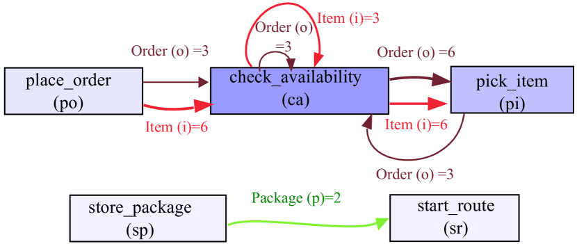
Figure 2: A simple DFM taken from Figure 1 for explaining the approach.

For simplicity, acronyms are used instead of the activities’ names, which are shown in parenthesis in the figure. For example, we will use $po$ instead of $place\_order$, $o$ instead of $order$, and so on.

Definition 1 (Directly-Follows Multigraph (DFM))

A Directly-Follows Multigraph (DFM) is a tuple $G=(OT,T,R,f)$, where:

• $OT$ is the set of object types,

• $T$ represents the set of tasks

• $R=(T\times OT\times T)$ is the set of relations connecting two tasks based on an object type. We call the first task the source and the second one the target, representing the task from/to which the relation starts/ends, respectively.

• $f\in R\rightarrow\mathbb{N}$ is a function that assigns a natural number, representing a frequency, to each relation.

Considering $\Theta\subseteq OT$ as a subset of object types, two operators on the graph’s tasks can be defined as follow:

• $\overset{\Theta}{\bullet}t$ represents the operator that retrieves the set of tasks from which there are relations to task $t$ for an object types within $\Theta$, i.e.,:

  $\overset{\Theta}{\bullet}t=\{t^{\prime}\in T|\exists_{\theta\in\Theta}(t^{\prime},\theta,t)\in R\}$.

• $t\overset{\Theta}{\bullet}$ represents the operator that retrieves the set of tasks to which there are relations from task $t$ for an object types within $\Theta$, i.e.,:

  $t\overset{\Theta}{\bullet}=\{t^{\prime}\in T|\exists_{\theta\in\Theta}(t,\theta,t^{\prime})\in R\}$.

Example 1

We can define the Directly-Follows Multigraph (DFM) for our running example in Figure 2 as $G=(OT,T,R,f)$, where:

• $OT=\{o,i,p\}$ is the set of object types.

• $T=\{po,ca,pi,sp,sr\}$ is the set of tasks.

• $R=\{(po,o,ca),(po,i,ca),(ca,o,ca),(ca,i,ca),\\ (ca,o,pi),(ca,i,pi),(pi,o,ca),(sp,p,sr)\}$ is the set of relations. $po$ is the source and $ca$ is the target of $(po,o,ca)$ relation.

• $f((po,o,ca))=3$, $f((po,i,ca))=6$, $f((ca,o,ca))=3$, $f((ca,i,ca))=3$, $f((ca,o,pi))=6$, $f((ca,i,pi))=6$, $f((pi,o,ca))=3$, $f((sp,p,sr))=2$ assigns frequencies to relations.

Examples of the operations based on the running example are given below:

• $\overset{\{i\}}{\bullet}ca=\{po,ca\}$ retrieves a set of tasks from which there are outgoing flows to check availability ($ca$) for object type item ($i$). Note that we can have different result if we change the object type, i.e., $\overset{\{o\}}{\bullet}ca=\{po,ca,pi\}$ which retrieves the set of tasks from which there is a relation to check availability ($ca$) for object type order ($o$).

• $ca\overset{\{i\}}{\bullet}=\{ca,pi\}$ and $po\overset{\{o\}}{\bullet}=\{ca\}$ retrieves a set of tasks to which there is a relation from check availability ($ca$) using item ($i$) object type and from place order ($po$) using order ($o$) object type, respectively.

	ca	pi	po	sp	sr
ca	1/3	2/3	0	0	0
pi	0	0	0	0	0
po	1	0	0	0	0
sp	0	0	0	0	0
sr	0	0	0	0	0

(a) Probability of relations for Item

	ca	pi	po	sp	sr
ca	1/3	2/3	0	0	0
pi	1	0	0	0	0
po	1	0	0	0	0
sp	0	0	0	0	0
sr	0	0	0	0	0

(b) Probability of relations for Order

	ca	pi	po	sp	sr
ca	0	0	0	0	0
pi	0	0	0	0	0
po	0	0	0	0	0
sp	0	0	0	0	1
sr	0	0	0	0	0

(c) Probability of relations for Package

TABLE I: The probability of each relation is represented through a matrix per object type, where rows and columns represent the source and target task, respectively.

To find similarities between the control flow for different case notions, we convert the Directly Follow Multigraph to Markov Directly Follow Multigraph, defined below. Also, we define a similarity measure that calculates how similar the control flow of the process model is with respect to two given object types.

Definition 2 (Markov Directly-Follows Multigraph (Markov DFM))

Let $G=(OT,T,R,f)$ be a DFM. $M=(G,p,sim)$ is a Markov DFM, where $p\in R\rightarrow[0$-$1]\subset\mathbb{Q}$ is a function that assigns a positive rational number between zero and one, representing the probability, to a relation. $sim\in OT\times OT\rightarrow[0$-$1]\subset\mathbb{Q}$ is a function that assigns a positive rational number between zero and one, representing the similarity, to an object types pair, where:

$$p\big{(}(t,\theta,t^{\prime})\big{)}\leftarrow\frac{f\big{(}(t,\theta,t^{\prime})\big{)}}{\sum_{\forall t^{{}^{\prime\prime}}\in t\overset{\{\theta\}}{\bullet}}{f\big{(}(t,\theta,t^{{}^{\prime\prime}})\big{)}}}$$ (1)

We can define the Markov Directly-Follows Multigraph (DFM) for our running example as $M=\big{(}G=(OT,T,R,f),p,sim\big{)}$. Let’s calculate $p$ using an example.

Example 2

• $p\big{(}(ca,o,pi)\big{)}=f\big{(}(ca,o,pi)\big{)}\Big{/}\Big{(}\sum_{\forall t\in ca\overset{\{o\}}{\bullet}}{f\big{(}(ca,o,t)\big{)}}\Big{)}$ $=6\Big{/}\Big{(}\sum_{\forall t\in{\{ca,pi\}}}{f\big{(}(ca,o,t)\big{)}}\Big{)}$ $=6\Big{/}\Big{(}f\big{(}(ca,o,ca)\big{)}+f\big{(}(ca,o,pi)\big{)}\Big{)}=6\Big{/}\Big{(}3+6\Big{)}=6/9=2/3$, which is the probablity of occurence of check availability given place order is occured for object type order in this model.

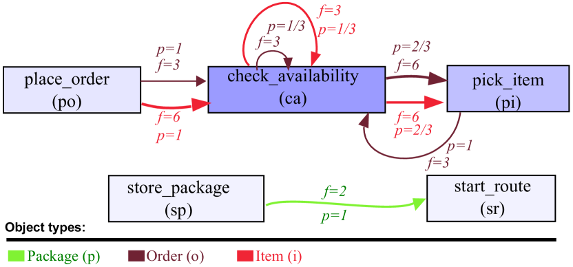
Figure 3: A Markov DFM of the DFM presented in Figure 2.

We can illustrate our graph based on this definition visually through Figure 3, where the frequencies and probabilities of relations are shown by $p$ and $f$, respectively. Note that probabilities can be represented by a matrix per object type, where rows and columns indicate the source and target tasks of a relation, as shown in TABLE I. This table also makes it easier to explain the similarity calculation using $sim$ function.

Example 3

As an example, let us to calculate $sim(i,o)$, where the probabilities of relations for item and order object types can be represented by $P_{i}$ and $P_{o}$ matrices as also shown in TABLE I.

• $P_{i}=\begin{bmatrix}\frac{1}{3}&\frac{2}{3}&0&0&0\\ 0&0&0&0&0\\ 1&0&0&0&0\\ 0&0&0&0&0\\ 0&0&0&0&0\end{bmatrix},P_{o}=\begin{bmatrix}\frac{1}{3}&\frac{2}{3}&0&0&0\\ 1&0&0&0&0\\ 1&0&0&0&0\\ 0&0&0&0&0\\ 0&0&0&0&0\end{bmatrix}$

The similarity function calculates the similarity accordingly:

• it calculates the denominator by summing up every element of $(P_{i}^{2}+P_{o}^{2})/2$, which is equivalent to $\sum_{\forall t_{1},t_{2}\in T}{\big{(}\cfrac{p(t_{1},i,t_{2})^{2}+p(t_{1},o,t_{2})^{2}}{2}\big{)}}$, which is eual to $\frac{37}{18}$.

• The similarity will then be calculated by $P_{i}\cdot P_{o}$ devided by the calculated denominator, which will be equal to $\frac{252}{333}=0.76$.

It is straightforward to calculate the similarity of Package with Item and also with Order in our running example. As the numerator will always be zero, the similarity will be zero. The similarity result of the process for each object type pair for this example can be shown as a matrix, represented in TABLE II. We call this matrix the similarity matrix.

	o	i	p
o	1.0	0.76	0.0
i	0.76	1.0	0.0
p	0.0	0.0	1.0

TABLE II: Calculated Similarity Matrix that shows the similarity of the process for object type pairs.

1

2 Algorithm discoverClusters($\big{(}(OT,T,R,f),p,sim\big{)},threshold$)

3       $clusters\leftarrow\{\}$;

4       foreach $\theta_{1},\theta_{2}\in OT$ do

5             if $sim(\theta_{1},\theta_{2})>=threshold$ then

6                   $X\leftarrow\bigcup_{C\in clusters}{\{C|\{\theta_{1}\}\subseteq C\ \vee\ \{\theta_{2}\}\subseteq C\}}$;

7                   $clusters\leftarrow clusters\backslash X\ \cup\ \{\{\newline \bigcup_{C\in X}{C}\ \cup\ \{\theta_{1},\theta_{2}\}\ \}\}$;

8            

9       return $clusters$;

10      

Algorithm 1 Clustering a Markov DFM algorithm

Algorithmus 1 defines how clusters of similar object types can be discovered from a Markov DFM given a threshold. It defines an empty set for clusters of object types (line 2). Then, for each pair of object types (line 3), if the similarity between them is greater or equal than the given threshold (line 4), it i) retrieves a union of sets of clusters that contains one of the object types (line 5), and ii) excludes the identified sets from the clusters and add all object types within these clusters in addition to two compared object types as a new cluster in the clusters set (line 6). It finally returns the identified set of clusters (line 7).

TABLE III shows the result of calling this algorithm for the running example using different thresholds in addition to the filtered similarity matrix.

	o	i	p
o	1.0	0.76	0.0
i	0.76	1.0	0.0
p	0.0	0.0	1.0

(a) 1 cluster when threshold=0, i.e., $\{\{i,o,p\}\}$

	o	i	p
o	1.0	0.76
i	0.76	1.0
p			1.0

(b) 2 clusters when threshold=0.01, i.e., $\{\{i,o\},\{p\}\}$

	o	i	p
o	1.0
i		1.0
p			1.0

(c) 3 clusters when threshold=0.77, i.e., $\{\{i\},\{o\},\{p\}\}$

TABLE III: Filtered similarity matrix and Identified clusters for the running example by setting different thresholds.

TABLE III(a) represents the result and the filtered similarity matrix when we call the algorithm by setting the threshold to zero. In this case, we will receive only one cluster that includes all object types. It is because the value for $sim(\theta_{1},\theta_{2})$ is always greater or equal to zero (line 4 of the algorithm), so all object types will be added to the returned cluster, so the result for our running example will be $\{\{i,o,p\}\}$.

TABLE III(b) represents the result and the filtered similarity matrix when we call the algorithm by setting the threshold to one percent. As seen in the filtered matrix, the relation between $p$ and other object types will be filtered as it is lower than the threshold. This result in the separation of these object types from others, so we will receive two clusters, i.e., $\{\{i,o\},\{p\}\}$.

TABLE III(c) represents the result and the filtered similarity matrix when we call the algorithm by setting the threshold to 77 percent. This result is $\{\{i\},\{o\},\{p\}\}$. It can be said that if an object type in the filtered matrix has similarities to others, they will be in the same cluster.

1

2 Algorithm tuneClusters($M,threshold,res$)

3       if $res=\{\}$ then

4             $res\leftarrow\{(0,discoverClusters(M,0))\}$;

5             $res\leftarrow res\ \cup\ \{(1,discoverClusters(M,1))\}$;

6             return $tuneClusters(M,0.5,res)$;

7            

8       else

9             if $(threshold,\_)\in res$ then

10                   return $res$;

11                  

12             else

13                   $CT\leftarrow discoverClusters(M,threshold)$;

14                   $res\leftarrow res\ \cup\ \{(threshold,CT)\}$;

15                  

16                  $u\leftarrow min\{i\ |\ \forall_{(i,-)\in res}\ i>threshold\}$;

17                   $l\leftarrow max\{i\ |\ \forall_{(i,-)\in res}\ i<threshold\}$;

18                  

19                  if $|\{C|\forall_{(t,C)\in res}\ t=u\}|\neq\ |CT|$ then

20                         $t\leftarrow round((threshold+u)/2,2)$;

21                         $res\leftarrow res\ \cup\ \{(t,discoverClusters(M,t))\}$;

22                        

23                  

24                  if $|\{C|\forall_{(t,C)\in res}\ t=l\}|\neq\ |CT|$ then

25                         $t\leftarrow round((threshold+l)/2,2)$;

26                         $res\leftarrow res\ \cup\ \{(t,discoverClusters(M,t))\}$;

27                        

28                  

29                  return $res$;

30                  

31            

32      

Algorithm 2 Cluster tuning algorithm

In practice, it is difficult to change the threshold to find all possible clusters manually, so Algorithmus2 tunes the threshold to identify all possibilities. This algorithm gets the $M$ (as a DFM), $threshold$, and $res$ - which is the result set representing the result of the previous tuning attempt. When calling this algorithm, the $res$ is an empty set as no tuning has happened. The algorithm performs recursively.

If it is the first time the algorithm is called, it discovers clusters for thresholds 0 and 1 and adds the result to the $res$. Then, it calls itself to tune the cluster discovery based on 0.5 thresholds and calculated $res$, and returns the result (line 5). If it is not the first time that Algorithm 2 is called, then it retrieves the lower- ($l$) and upper- ($u$) bounds of threshold in $res$. If the number of clusters in the current threshold is not equal to $u$, then it discovers a cluster for a threshold in between. To avoid running this algorithm infinitely, we calculated the value in between by rounding the value by having two digits after the decimal points. It does the same for $l$, and it returns the result finally. This algorithm tune the threshold parameter through a half-interval search.

IV Implementation

The approach is implemented and is available as a part of a python library, called processmining. The source is available in Github , and the library is available in PyPI - which enables users to install and use it easily by running the pip command , if python and PM4Py are installed. The library aims to provide more functionalities to perform process mining using python and other libraries like PM4Py. The codes to repeat the running example and evaluation can be found at Github .

Figure 4 shows the result of cluster tuning for DFM in Figure 1, where it discovered four sets of clusters. In this figure, the x- and y- axes represent the threshold and number of retrieved clusters for the threshold parameter, respectively.

Figure 4: The result of cluster tuning for Figure 1 using implemented library.

(a) 0 threshold

(b) 0.16 threshold

(c) 0.57 threshold

(d) 0.68 threshold

Figure 5: The similarity matrices for identified clusters in Figure 4.

The similarity matrix of these sets of clusters is plotted in Figure 5, where each sub-figure shows the similarity matrix for one threshold. As it can be seen from the sub-figures, the number of clusters in each set will be changed by changing the threshold. For example, if we set the threshold to 0.16, then it will return two clusters, i.e., $\{\{Item,Order\},\{Package,Route\}\}$. Flattening the OCEL based on these clusters can help discover process models with similar control behavior, as shown in Figure 6. This figure is made intentionally small only to show how the interconnected DFM in Figure 1 will look in general when flattening the log based on similar object types. Such flattening still enables the study of the connection among similar object types, yet focusing on the related ones. The code for reproducing this experiment can be found in the Github .

(a) DFM for the cluster that include Order and Item object types

(b) DFM for the cluster that include Package and Route object types

Figure 6: Discovered DFMs based on two identified clusters by a similarity threshold of 0.16. The figure is made intentionally small just to show supporting the separation of similar object types.

V Evaluation

This section evaluates the presented approach using the given implementation on a Purchase to Pay (P2P) object-centric event log file. For the evaluation, SAP ERP IDES instance - P2P log file is used which is provided by http://ocel-standard.org [7]. This log file records the events for the Purchase to Pay process, and it contains 24,854 events and 9 object types.

These steps are followed to evaluate the approach. First, sets of clusters are identified by applying this technique. Second, some of the identified clusters are evaluated by flattening the log based on clustered object types. Third, the log is flattened based on each object type, and a process model is discovered using the inductive miner for each flattened log. For each pair of object types, their corresponding discovered models using inductive miner are compared using the footprint analysis technique. Finally, the result of the footprint analysis is compared with identified clusters.

V-A Cluster discovery

This section presents the result of first and second steps in evaluating the proposed approach. Figure 7(a) shows the result of threshold parameter tuning, where four different thresholds have been identified to discover different sets of clusters. The first threshold, i.e., zero, will classify all object types into one cluster, and the last one will classify each object type in one cluster. Thus, we only present the two similarity matrices for the two remaining sets of clusters in Figure 7(b) and (c).

(a) threshold parameter tuning

(b) threshold=0.01

(c) threshold=0.31

Figure 7: Cluster discovery result for p2p process.

As can be seen in Figure 7(a), setting the threshold to 0.01 will result in 7 clusters. The similarity matrix in Figure 7(b) shows that all object types except EBELN, EBELN_EBELP, and MATNR are classified into their own clusters, meaning that they do not share any similar behavior.

This finding can be validated by flattening the log based on these object types and discovering one process model, shown in Figure 8(a). The process is made intentionally small to show that there are unconnected tasks in addition to some disconnected control flow for different object types. The result confirms that these objects do not share similar behavior. Indeed, except for BANFN and BELNR object types, we do not see any occurrence of two consequent events for other object types. The control flow for BANFN and BELNR object types also do not share any task, so they are distinct.

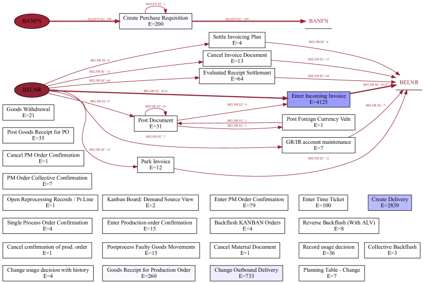
(a) Discovered DFM showing distinct behaviour of identified clusters when setting threshold to 0.01.

(b) Discovered DFM showing similarity between behaviour for EBELN and EBELN_EBELP object types.

Figure 8: Discovered DFM for different object types. These processes are made intentionally small to show the validity of the result, and they are not meant to be read in detail.

Increasing the threshold to 0.31 will discover a cluster with two object types, i.e., EBELN, EBELN_EBELP. The process model, which is discovered by flattening the log based on these two object types, shows very similar behavior among them (see Figure 8(b)).

V-B Footprint analysis for flattened logs

This section presents the result of the remaining steps in evaluating the proposed approach. Figure 9 shows the result of the conformance checking, where rows and columns represent object types, and cells represent the conformance of discovered process models using inductive miner by flattening the log - based on each object type.

Figure 9: The calculated similarity between discovered process models using inductive miner by flattening the log based on each object type.

As it can be seen, the highest difference in footprints belongs to MATNR, which has been identified as one cluster when setting the threshold to 0.31. Taking this object type apart, the footprint difference for EBELN and EBELN_EBELP has the highest difference with other object types while minimum difference to each other. This result aligns with the identification of the cluster that contains these two object types when setting the threshold between 0.31 and 0.94. The code for this experiment is available in Github .

VI Conclusion

This paper introduced a new approach to cluster similar case notions by defining Markov Directly-Follow Multigraph. The graph is used to define an algorithm for discovering clusters of similar case notions based on a threshold. The paper also defined a threshold tuning algorithm to identify sets of different clusters that can be discovered based on different levels of similarity. Thus, the cluster discovery does not merely rely on analysts’ assumptions. The approach is implemented and released as a part of a python library, called processmining, and it is evaluated through a Purchase to Pay (P2P) object-centric event log file. Some discovered clusters are evaluated by discovering Directly Follow-Multigraph by flattening the log based on the clusters. The similarity between identified clusters is also evaluated by calculating the similarity between the behavior of the process models discovered for each case notion using inductive miner based on footprints conformance checking.

This approach can be used to define an object-centric process discovery algorithm that takes the similarity of object types into account when discovering process models from object-centric event logs, which will be a future direction of this work.

References

- [1] J.N. Adams and W.M.P. van der Aalst. Precision and fitness in object-centric process mining. In 2021 3rd International Conference on Process Mining (ICPM), pages 128–135. IEEE, 2021.
- [2] A. Augusto, R. Conforti, M. Dumas, M. La Rosa, and A. Polyvyanyy. Split miner: automated discovery of accurate and simple business process models from event logs. Knowledge and Information Systems, 59(2):251–284, 2019.
- [3] A. Berti, A.F. Ghahfarokhi, G. Park, and W.M.P. van der Aalst. A scalable database for the storage of object-centric event logs. In Proceedings of the ICPM Doctoral Consortium and Demo Track 2021. CEUR Workshop Proceedings, 2021.
- [4] A. Berti, G. Park, M. Rafiei, and W.M.P. van der Aalst. An event data extraction approach from sap erp for process mining. In International Conference on Process Mining, pages 255–267. Springer, Cham, 2021.
- [5] A. Berti, S.J. van Zelst, and W.M.P. van der Aalst. Process mining for python (pm4py): Bridging the gap between process- and data science. In Proceedings of the ICPM Demo Track 2019. CEUR Workshop Proceedings, 2019.
- [6] S. Esser and D. Fahland. Multi-dimensional event data in graph databases. Journal on Data Semantics, 10(1):109–141, 2021.
- [7] A.F. Ghahfarokhi, G. Park, A. Berti, and W.M.P. van der Aalst. Ocel: A standard for object-centric event logs. In European Conference on Advances in Databases and Information Systems, pages 169–175. Springer, 2021.
- [8] A.F. Ghahfarokhi and W.M.P. van der Aalst. A python tool for object-centric process mining comparison. In Proceedings of the ICPM Doctoral Consortium and Demo Track 2021. CEUR Workshop Proceedings, 2021.
- [9] A. Jalali, P. Johannesson, E. Perjons, Y. Askfors, A. Rezaei Kalladj, T. Shemeikka, and A. Vég. dfgcompare: a library to support process variant analysis through markov models. BMC medical informatics and decision making, 21(1):1–13, 2021.
- [10] A. Jalali, F.M. Maggi, and H.A. Reijers. A hybrid approach for aspect-oriented business process modeling. Journal of Software: Evolution and process, 30(8):e1931, 2018.
- [11] Amin Jalali. Graph-based process mining. In Sander Leemans and Henrik Leopold, editors, Process Mining Workshops - in conjuction with the International Conference on Process Mining, pages 273–285. Springer, 2020.
- [12] M. La Rosa, P. Wohed, J. Mendling, A.HM ter Hofstede, H.A. Reijers, and W.M.P. van der Aalst. Managing process model complexity via abstract syntax modifications. IEEE Transactions on Industrial Informatics, 7(4):614–629, 2011.
- [13] J. Meyer, J. Reimold, and C. Wehmschulte. Associative intelligence for object-centric process mining with mpm. In ICPM 2021 Doctoral Consortium and Demo Track 2021. CEUR Workshop Proceedings, 2021.
- [14] F. Taymouri, M. La Rosa, and J. Carmona. Business process variant analysis based on mutual fingerprints of event logs. In International Conference on Advanced Information Systems Engineering, pages 299–318. Springer, 2020.
- [15] F. Taymouri, M. La Rosa, M. Dumas, and F.M. Maggi. Business process variant analysis: Survey and classification. Knowledge-Based Systems, 211:106557, 2021.
- [16] W.M.P. van der Aalst. Process mining: Overview and opportunities. ACM Transactions on Management Information Systems (TMIS), 3(2):1–17, 2012.
- [17] W.M.P. van der Aalst. Object-centric process mining: Dealing with divergence and convergence in event data. In International Conference on Software Engineering and Formal Methods, pages 3–25. Springer, 2019.
- [18] W.M.P. van der Aalst. A practitioner’s guide to process mining: limitations of the directly-follows graph, 2019.
- [19] W.M.P. van der Aalst and A. Berti. Discovering object-centric petri nets. Fundamenta informaticae, 175(1-4):1–40, 2020.
- [20] S.K. vanden Broucke and J. De Weerdt. Fodina: a robust and flexible heuristic process discovery technique. decision support systems, 100:109–118, 2017.
- [21] AJMM Weijters and J.T.S. Ribeiro. Flexible heuristics miner (fhm). In 2011 IEEE symposium on computational intelligence and data mining (CIDM), pages 310–317. IEEE, 2011.