Shape fluctuations and radiation from thermally excited electronic states of boron clusters

Abstract

The effect of thermal shape fluctuations on the recurrent fluorescence of boron cluster cations, B${}_{N}^{+}$ ($N=9-14$), has been investigated numerically, with a special emphasis on B${}_{13}^{+}$. For this cluster, the electronic structures of the ground state and the four lowest electronically excited states were calculated using time-dependent density functional theory, and sampled on molecular dynamics trajectories of the cluster calculated at an experimentally relevant excitation energy. The sampled optical transition matrix elements for B${}_{13}^{+}$ allowed to construct its emission spectrum from the thermally populated electronically excited states. The spectrum was found to be broad, reaching down to at least 0.85 eV. This contrasts strongly with the static picture, where the lowest electronic transition happens at 2.3 eV. The low-lying electronic excitations produce a strong increase in the rates of recurrent fluorescence, calculated to peak at $4.6\times 10^{4}$ s^-1, with a time-average of $8\times 10^{3}$ s^-1. The average value is one order of magnitude higher than the static result, approaching the measured radiation rate. Similar results were found for the other cluster sizes. Furthermore, the radiationless crossing between the ground-state and the first electronic excited state surfaces of B${}_{13}^{+}$ was calculated, found to be very fast compared to experimental time scales, justifying the thermal population assumption.

I Introduction

Thermal radiation, long considered to be restricted to vibrational cooling, has also been demonstrated to occur from electronically excited states, via the so-called recurrent fluorescence (RF) or Poincare radiation. This type of radiation is attracting increasing attention as more and more molecules and clusters are recognized as emitters, and in part also stimulated by the implications for astrophysics. To date, recurrent fluorescence has been observed in fullerenes [1, 2], where the effect was first seen, as well as in polycyclic hydrocabon (PAH) molecules [3, 4] and in clusters of several metallic and semiconductor elements. For very recent results of direct astrophysical relevance, please see [5]. Moreover, RF is known to be present in both anionic, neutral and cationic species, highlighting its general relevance at the nanoscale [6].

The existence of this type of radiation follows from time reversal once the presence of radiationless transitions is established. Radiationless transitions connect different Born-Oppenheimer surfaces, allowing for the phenomenon of internal conversion (IC), in which electronic energy is converted into vibrational motion on the electronic ground state. Time reversal requires that the reverse process, i.e., inverse internal conversion (IIC), is also allowed, which means that in principle any excited electronic state that undergoes IC can be reached non-radiatively from the electronic ground state [7]. In RF, photon emission occurs from electronically excited states that are populated via IIC. As the radiationless transitions are very well established for a number of molecules, the main concern about the presence of RF has been the question to which degree molecular electronically excited states are populated thermally. The experimental evidence is now strongly in favor of the existence of RF, and the theoretical results here will add to this evidence.

Although RF was predicted several decades ago [8, 9, 10], photons emitted by this mechanism from mass selected clusters and molecules were only observed recently, for the molecules C${}_{6}^{-}$ [11], C${}_{4}^{-}$ [12] and naphthalene cations[13]. The vast majority of other studies of RF have deduced its presence from its quenching effect on the unimolecular decays of the emitting particles (see ref. [6] for a review of this method). The involved unimolecular signature decays can be the loss of atoms or larger fragments or, for anions and neutrals, thermal electron emission. The observed time scales for RF vary strongly with the system, from the highest rate constants found so far of $10^{6}$ s^-1 for cationic gold [14] and cobalt [15] clusters, to close to the typical vibrational radiative time scales that are four orders of magnitude slower.

Two of the three cases where RF photons have been detected directly from mass selected molecular beams (C${}_{6}^{-}$ and C${}_{4}^{-}$) employed a narrow detection window centered on the wavelengths where the particles in their ground-state absorb light [11, 12]. The selective detection of this narrow spectral region was motivated by the desire to establish the origin of the photons. In the experiment measuring the spectrum of photons emitted from naphthalene, a significant broadening relative to the ground state absorption spectrum was observed [13].

Such broadening is not unexpected and can be understood qualitatively as the consequence of the varying geometric structures sampled by the thermal excitation, with the concomitant sampling of transition energies and oscillator strengths across the involved potential energy surfaces. Spectral smearing is thus expected to be intrinsic to the RF phenomenon.

The measurements on the quenching effect of radiation on competing processes usually only provide a single value in the form of the photon emission rate constant. This value is the thermally averaged photon emission rate constant at the total excitation energy where it equals the unimolecular decay rate constant, $k_{\rm ph}\sim k_{\rm unimol}$, because this defines the energy where the emission rate constant is measured (see Ref. [6] for a detailed explanation of this).

Electronically excited states characterized spectroscopically tend to misrepresent emission rate constants, because these data usually only pertain to the very limited part of configuration space that correspond to excitation from a ground state geometry. In contrast, highly excited and free-roaming species will explore much wider regions of configuration space. The effective thermally-averaged transition energies and oscillator strengths will therefore in general differ from values derived from low temperature spectroscopic data. Hence, the thermal exploration of potential energy surfaces provides information on their shape. The investigation of this effect for well characterized systems is the main motivation of this work.

The system chosen for this study is boron clusters, for which the effective (averaged) photon emission rate constants, but no emission spectra, have been measured upon laser excitation [16]. The experimentally measured radiation rate constants for these clusters are significant, reaching for example $6\times 10^{4}$ s^-1 for B${}_{13}^{+}$ and $5\times 10^{5}$ s^-1 for B${}_{9}^{+}$. These high values strongly suggest that the emission mechanism is RF, and indicate that the clusters possess optically active electronically excited states at low energies. In this work, most attention is given to B${}_{13}^{+}$, for which the ground-state geometry has been determined based on spectroscopic experiments [17]. We expect that the general picture revealed for this cluster apply equally well to other boron clusters which, noted in passing, by themselves are very interesting objects, with remarkable planar geometries, possessing fascinating fluxionality properties [17, 18, 19, 20, 21]. Moreover, low-lying quasi-degenerate electronic states in boron clusters have also been shown to play an important role in their electron wavepacket dynamics [22].

II Thermal shape fluctuations and electronic structure

The central idea of the work is illustrated schematically in Fig. 1. For a cluster in its ground-state geometry with a large energy difference between the electronic ground-state and the first electronic excited state (left part of the figure), an optical transition between such states will translate into a small radiation rate [23]. This is not consistent with the observed high photon emission rate constants of, for example, laser-excited boron clusters [16]. However, the geometry of highly excited clusters will fluctuate over time as illustrated schematically on the right side of the figure. This dynamics can reduce the energy difference between the ground state and the electronically excited states. This will cause a higher thermal population of the excited states, which results in faster photon emission [6].

An explicit calculation of this reduction of the excitation gap (electronic transitions modified by structural deformation) has already been performed for Al${}_{13}^{-}$, based on a spherical box potential of finite depth, undergoing a spheroidal distortion [24], albeit without any considerations of thermal radiation. The work showed a reduction in the HOMO-LUMO gap energy caused by this structural deformation.

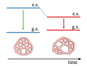
Figure 1: Schematic illustration of the possible reduction of the energy difference between the ground state and the first excited state of a cluster, caused by temperature-induced geometrical deformations.

III Computational details

To investigate this thermal deformation-induced effect in boron clusters, we have performed Molecular Dynamics (MD) simulations with potential energies calculated with Density Functional Theory (DFT). The MD simulations are standard integration of the Newtonian equations of motion. Specifically, the linear-response time-dependent DFT (LR-TDDFT) formalism was employed in order to compute the lowest lying low spin excitations in B${}_{N}^{+}$ ($N=9-14$) clusters. For B${}_{13}^{+}$ four electronic excitations were calculated. Due to the long computer times required for these calculations, however, only two electronic excitations were computed for the other cluster sizes. The computations were performed using the CAM-B3LYP exchange-correlation functional [25], in combination with the def2-SVP basis set [26]. The relatively small basis set allows for relatively long MD simulation times. CAM-B3LYP was found to give excellent excitation energies for boron clusters, based on a benchmarking with coupled cluster theory (EOM-CCSD) [27], while our computations showed only a small difference in the excitation spectra between the split valence def2-SVP and the triple zeta valence def2-TZVP basis sets. For example, in B${}_{13}^{+}$, the energy of the first vertical electronic excitation from the lowest energy singlet geometry (S₀ $\rightarrow$ S₁) is calculated to be 2.27 eV and 2.25 eV, for def2-SVP and def2-TZVP, respectively.

The ground state geometry of B${}_{13}^{+}$ was experimentally identified in Ref. [17]. The molecular dynamics simulations on the first excited low spin potential energy surface were performed with a microcanonical ($NVE$) ensemble, with initial coordinates of the lowest energy structure on the ground state potential energy surface (vertical excited state) and with initial nuclear velocities selected from a canonical energy distribution.

The choice of using a temperature for a microcanonical simulation was made because the decay dynamics of the beam defines an effective, microcanonical temperature, and this temperature can be determined. The relation was suggested by Gspann [28] and developed by Klots [29, 30]. It reads (with $k_{\rm B}=1$):

$$T=D(1/\ln(\omega_{\rm a}t)+1/2C_{\rm v}).$$ (1)

The parameters in this expression are the evaporative activation energy, $D$, the frequency factor of the unimolecular rate constant, $\omega_{\rm a}$, the experimental measurement time $t$, and the cluster’s heat capacity, $C_{\rm v}$, given in units of Boltzmann’s constant. In these experiments the time $t=1/k_{\rm p}$ is the value at which the thermal photon emission rate constant is equal to the unimolecular fragmentation rate constant, and the time is therefore set to this value. In brief, at higher excitation energies, instantaneous fragmentation is the dominant cooling channel, whereas at lower values, fragmentation is exponentially suppressed. Hence

$$T=D(1/\ln(\omega_{\rm a}/k_{\rm p})+1/2C_{\rm v}).$$ (2)

and this is therefore the energy at which the photon emission rate constant is determined experimentally.

For completeness we should mention that this temperature is the microcanonical value, but the difference to the canonical temperature can be ignored here. For more details on this the reader can consult [23], and ref. [31] for the meaning of the microcanonical temperature.

The value found for B${}_{13}^{+}$ is 3855 K. In energy units this temperature is 0.33 eV. This temperature together with the speeds selected at random from the Maxwell-Boltzmann distribution gave the total nuclear kinetic energy of 5.61 eV, close to the canonical average value of 5.48 eV. The simulations were started from the ground state geometry and the first excited state. The energy of that state, 2.27 eV, should be added to the total energy.

The potential energy surface of B${}_{13}^{+}$ and the possible emission routes were explored using adiabatic molecular dynamics simulations on the S₁ state. The molecular dynamics (MD) simulations propagate the system in time by solving the classical equations of motion for the nuclei, while calculating the potential energy on all surfaces point-by-point with the density functional theory (DFT) calculations mentioned above. The S₁ surface was chosen as a representative of an emitting surface, but the specific choice is not critical for the exploration of the phase space. The simulations were tested with two different time-steps, 0.02 and 0.1 fs. The results were very similar, and longer simulations were therefore conducted with the latter value.

The small S₀-S₁ energy differences that are calculated (see Section III) imply that non-adiabaticity is important. An accurate description of such effects is computationally demanding, and non-adiabatic effects are therefore explored only for B${}_{13}^{+}$. To calculate these effects, and ensure that the computations are reliable, three different methods were used, namely spin-flip Density Functional Theory (SF-DFT) employing the recommended Becke half & half LYP (SF-BH&HLYP) functional and the def2-SVP basis, the spin-flip equation of motion coupled clusters singles and doubles (SF-EOM-CCSD) [32] and the def2-SVP basis set, and the extended multi-state second order complete active space (XMS-CASPT2) method [33], based on state-averaged CASSCF reference involving the lowest three singlet states and the TZVP basis set. It has been shown recently that XMS-CASPT2 and SF-BH & HLYP yield similar results for conical intersections [34]. The DFT, SF-DFT and SF-EOM-CCSD computations were performed using the Q/Chem 5.2 and 5.4 program packages [35], while the XMS-CASPT2 computations were completed using the BAGEL code [36], with results available in the Supporting Information (Table S1).

These computations make it possible to estimate the transition rate through the minimum energy crossing points toward the S₀ and the S₁ state. The magnitude of these time constants indicates that on the much longer microsecond experimental time scale the excited states can reach thermal populations. This allows us to sample the phase space using molecular dynamics simulations and estimate the radiative emission rate from the thermal populations of the excited states

Nonadiabatic couplings (NACs) can be computed by differentiating the electronic wavefunctions with respect to the nuclear coordinates. Here we used the pseudo-wavefunction approach to compute the NACs analogously [37, 38], using TDDFT employing the SF-BH&HLYP method, as implemented in the Q-Chem software [35].

IV Dynamics of electronic excited states

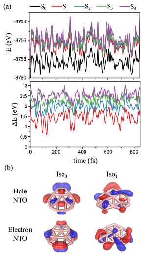
Figure 2: (a) Top: Energies of the electronic excited states S_i ($i=1-4$) and the ground state S₀ of B${}_{13}^{+}$, as a function of simulation time. Bottom: Energy difference between each electronic excited states and the ground state. (b) Cluster geometries and the isosurfaces (isovalues: 0.05) of the leading Natural Transition Orbital (NTO) pairs for the S₀ ground state at the lowest energy geometry (initial structure, iso₀ at $t=0$) and at a low energy structural isomer (iso1 at an optimized intermediate structure, c.f. Fig. 3).

The top panel of Figure 2a shows the energies of the four lowest electronic states, in addition to the S₀ ground-state, along the molecular dynamics trajectory for B${}_{13}^{+}$. The bottom panel presents the energies of the excited electronic states relative to the energy of S₀. Interestingly, the four excited states and the ground-state show a correlated pattern with time. As seen from the figure, the energy difference between the first excited state and the ground state (red curve) at the initial configuration, and thus the lowest vertical excitation energy in the ground state geometry, is over 2 eV. This energy difference reduces to below 1 eV at several later moments, showing the possibility of emission of lower energy photons. Whether this possibility is realized depends on whether the states are thermally populated, which in turn depends on the excited state energy relative to the ground state energy and not on their difference with respect to the simultaneous energy of S₀.

Geometry optimization starting from the regions with a small S₀-S₁ energy difference confirmed the existence of a structural isomer with an energy which is only slightly higher than the lowest energy isomer, as shown in Figure 2b. In both cases, the excitation from the ground to the first excited state can be described approximately by a single electron configuration, which involves the formal electron transfer from the highest occupied molecular orbital (HOMO) to the lowest unoccupied molecular orbital (LUMO). This is accurately reflected by the fact that the excitation can be well described using a single natural transition orbital (NTO) pair, where the shape of the hole and the electron NTOs resemble those of the HOMO and LUMO, respectively. It is clearly visible that the shapes of the electron and hole NTOs follow the distortion of the cluster shapes towards the low energy structural isomer.

The analysis shown so far involves the adiabatic approximation i.e. the MD trajectory was propagated on a single potential energy surface, with the different surfaces computed independently. However, it has been shown that the dynamics of boron clusters also involves non-adiabatic effects [22], including the presence of several conical intersections and avoided crossings. These were therefore investigated in more detail.

V Non-adiabatic effects

The relevance of excited states in the description of the radiative cooling of a cluster or molecule is to some degree a question of time scales. States need to be populated. To assess whether excited states are populated, the time scale determined by the coupling between the should be compared with the microsecond or longer experimental time scale at which the populations are monitored, i.e. the time at which the radiative cooling is measured. This long time scale puts very mild conditions on the coupling.

In the current section we explore a part of the potential energy surface, at which the relative populations of the Born-Oppenheimer (BO) states are calculated by calculating non-adiabatic couplings. As the typical time scale of RF cannot be attained using conventional molecular dynamics simulations, we explore the stationary (zero derivative) points and the crossing points between the lowest two singlet states in the neighborhood of the lowest energy geometry. The crossing points on the computed trajectories (described in the caption of Figure 3) clearly show the possibility of non-radiative transitions between the two lowest singlet states. Crossings between higher excited states should also present, but these do not alter the results found here for the two lowest states fundamentally.

The small energy difference between the S₀ and the S₁ states of B${}_{13}^{+}$ will induce large non-adiabatic couplings, and also generate conical intersections. Here, we have optimized the initial and the isomeric geometries of B${}_{13}^{+}$, and systematically explored the two adjacent minimum energy crossing points (MECP, Figure 3). The MECPs are the lowest energy points on the line defining the intersection of the two surfaces. The variations in potential energies are much below the energy used in the MD simulations. Hence the crossing configurations shown are well within energetic reach. The computations were performed using SF-TDDFT, which was motivated by the fact that unlike the conventional TDDFT, this method correctly describes the topology of the conical intersections involving the S₀ state [39]. To further assess the accuracy of our computations, we recomputed the geometries and energies of the minima and the MECPs using SF-EOM-CCSD and XMS-CASPT2 methods (see Table S1 in the Supporting Information).

To illustrate the topology of the S₀ and the S₁ potential energy surfaces we computed the linar synchronous transit paths (i.e. linear interpolation in Cartesian coordinates) between the minima and the MECPs shown in Fig. 2(b).

The abscissa in both curves is the root mean square deviation of the atomic positions compared to Iso₀. Note that this figure is not a trace of the MD simulation, and that the data do not enter the statistics derived from that simulation. Figure 3 shows that there are several MECPs between the S₀ and the S₁ potential energy surfaces on this curve. The energies of those two states at the isomeric structures are not much higher than the ground state energy in the lowest energy minimum, and will thus be easily accessible at the experimental conditions of radiative cooling studies of excited clusters in molecular beams, as discussed above. This is confirmed by calculations of the rate coefficients for crossing, involving thermally activated reactions (see Supporting Information for details).

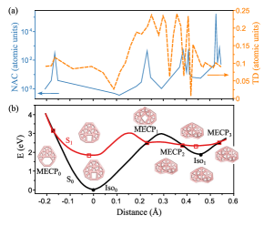
Figure 3: (a) Magnitude of the transition dipole moments (TD) and the non-adiabatic coupling vectors (NAC, logarithmic scale), both in atomic units (Hartree/$a_{0}$ for NAC) along the constructed linear synchronous interpolation curve described in the main text. The abscissa is the root-mean-square of the stretched nuclear coordinates. (b) Geometries and energies along the path between the lowest energy Iso₀ and the intermediate Iso₁ geometries, and the adjacent minimum energy crossing points of the two lowest potential surfaces (S₀ and S₁). Stationary and minimum energy crossing points are indicated by dots. The paths from the isomer Iso₀ to MECP₀ and from Iso₁ to MECP₃ are stretched for visibility. Calculations are performed at the SF-BH&HLYP/def2-SVP level. The S₀-S₁ excitation energy at zero abscissa differs from the previously quoted 0.225 eV and 0.227 eV because the value here is not vertical i.e. the S₀ and S₁ geometries are different, except in the case of the MECPs.

The magnitude of the transition dipole moment between the S₀ and the S₁ states determines the rate of photon emission via the electronic transition between the two states, while the magnitude of the non-adiabatic coupling indicates the efficiency of the non-radiative relaxation and the excitation. It is clearly seen from Figure 3 that, as expected, the probability of the non-radiative relaxation or excitation is very high in the vicinity of the MECPs, as the magnitude of the non-adiabatic couplings increases by factors up of $\sim$ $10^{2}$ to $10^{4}$ compared to the original value, while the magnitude of the transition dipole moment increases by a more modest factor of 2-3. Hence, although photon emission is more probable near MECPs and the conical intersections that may be present than elsewhere, the non-radiative coupling is much more enhanced at these points. In this connection it is worth noting that non-adiabatic wavefunction dynamics of boron clusters have indicated the presence of several conical intersections and frequently occurring high non-adiabatic couplings [22]. Transition state theory calculations (see the Supporting Information for more details) show that the transition rate at the MECP₁ is approximately $4\times 10^{9}$ s^-1 and thus well within the microsecond time scale of the emission. These results showing a rapid exchange of energy between the electronic ground-state and the first-excited state of B${}_{13}^{+}$ strongly support the suggestion that photon emission in boron clusters proceeds via IIC and recurrent fluorescence in boron cluster cations.

VI Microcanonical averaging

The combination of time-dependent energies of the electronic state S₀ ($i=0-4$) energies with the oscillator strengths $f_{i}$ for the transitions, allow the construction of the emission spectrum of B${}_{13}^{+}$ for the sampled geometries. In the rapid equilibration scheme relevant here the statistical weight of an excited state is given by the level density of the kinetic energy for that geometry. With $E$ the total (conserved) excitation energy relative to the absolute ground state, and $V_{i}(x)$ the potential energy of the state $i$ ($i=0-4$) in the geometry labeled by $x$, the unnormalized populations of the states ($g_{i}$) are, with $s\equiv 3N-6$, equal to

$$g_{i}(x)=c(E-V_{i}(x))^{s/2-1},i=0,1,....$$ (3)

This expression is simply the density of states for $s$ momenta with a total energy $E-V_{i}(x)$ and the sampled geometry in the simulated microcanonical ensemble. The assumption is the fundamental postulate of thermodynamics that all quantum states are populated with equal probability. The constant $c$ is identical for the different states, as are the number of degrees of freedom of the nuclear motion, $s$. The population of the state $i$ is therefore

$$p_{i}=\frac{g_{i}(x)}{\sum_{j=0}g_{j}(x)},$$ (4)

where $j$ runs over all relevant states. For values of $V_{i}(x)$ exceeding $E$, obviously state $i$ is unpopulated.

With the oscillator strengths and energies of the surfaces the rates of photon emission can thus be computed as a function of time along the trajectory. At each point the photon emission rate constant from state $i$ ($i-1-4$) is given by [23]:

$$k_{\rm p}^{i}=7.421\times 10^{-22}{\rm Hz}f\nu_{0}^{2}p_{i}$$ (5)

In this expression, $f$ is the oscillator strength and $h\nu_{0}$ the transition energy. For B${}_{13}^{+}$ the total rate constant is then calculated as the sum of the four $k_{\rm p}^{i}$ values (see Figure 2a). For the other cluster sizes two electronic excited states were computed.

VII Emission spectra

The result for B${}_{13}^{+}$ is presented in Figure 4a), where the total radiation rate constant is shown as a function of MD simulation time. The figure also shows the effect of the number of excited states included in the calcuation. The values vary strongly with time, as expected from the pronounced dependence of the energy of the excited states seen in Fig. 2. The rate constant reaches significantly higher values than for the static picture in the ground-state geometry, as highlighted by the scale on the right hand axis of the figure, where $k_{\rm p}$ is normalized with respect to the rate at zero kelvin.

Another important observation from this result is the quite high absolute values that are reached along the simulation (axis on the left), peaking at $4.6\times 10^{4}$ s^-1. This value is very close to the experimental result in Ref. [16], which is $(6.1\pm 2.8)\times 10^{4}$ s^-1. In Figure 4b, the distribution of $k_{\rm p}$ values is depicted and fitted by a log-normal distribution. This allows an estimation of the average $k_{\rm p}$, yielding the value $8\times 10^{3}$ s^-1. As discussed below, this improved estimate is still most probably an underestimate of the values that are generated by the RF mechanism.

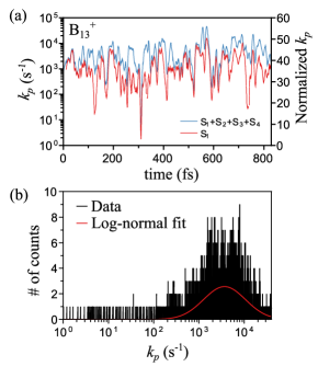
Figure 4: (a) Time-dependent radiation rate constant calculated for B${}_{13}^{+}$ at an initial kinetic energy corresponding to the temperature of 3855 K. The red curve shows the radiation constant when only emission from S${\rm 1}$ is considered. The blue gives the emission rate constant for the first four excited states. (b) Distribution of $k_{\rm p}$ for B${}_{13}^{+}$ as derived from the time-dependent behaviour in (a). A log-normal distribution is used to fit an average $k_{\rm p}$ value.

Based on the energies and oscillator strengths calculated for the four electronic states of B${}_{13}^{+}$, an emission spectrum is constructed, as presented in Figure 5. The spectrum is calculated as the sum over the spectra produced by emission from the four excited states with the expression for each of them equal to

$$Y_{i}(h\nu)=\frac{\sum_{j}^{\prime}k_{i,j}}{\Delta h\nu N},$$ (6)

where $N$ is the total number of sampled points and the primed sum over $j$ is over the points where the photon energy is found in the interval between $h\nu$ and $h\nu+\Delta h\nu$. The total spectrum is then

$$Y(h\nu)=\sum_{i}Y_{i}(h\nu).$$ (7)

It shows bands of significant widths for each of the excited states, spanning between 0.85 eV and 3 eV. Note that the lower energy of 0.85 eV is the value observed in the relatively short simulations. The true lower limit is most likely much lower, approaching close to zero (see Fig. 3).

This high-temperature spectrum is very different from the static picture calculated with LR-TDDFT at the ground-state geometry (shown in the inset). That spectrum is composed of a small set of discrete transitions, with the first occurring at 2.27 eV. It is worth reiterating that the spectrum in Figure 5 represents the configurations encountered in the MD simulation. The true lower energy cutoff will be lower, as demonstrated by the level crossings seen in Fig. 3. The time-average, energy integrated total oscillator strength at the elevated temperature shown in Fig.5 is lower than the static values, but not significantly so.

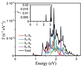
Figure 5: Emission spectrum of B${}_{13}^{+}$ at the microcanonical temperature of 3855 K. The spectrum is calculated with the difference of energy of the electronic states to the absolute ground state, yielding the populations of the excited states, and the oscillator strengths of those transitions. The sum $\sum_{i}Y_{i}$ is shown as a black line. The static emission spectrum, calculated with LR-TDDFT on the ground-state geometry of the cluster, is shown in the inset. This is constructed by assuming Gaussian functions around each transition, with an artificial width of 0.05 eV.

The analysis performed for B${}_{13}^{+}$ was also conducted for the other boron clusters of the sizes $N=9-12,14$. The results for these clusters are included in the summary of all the radiative rate constants shown in Figure 6,. The figure compares the MD time-average rates obtained from the computations in this work with the experimental data of Ref. [16]. Additionally, the maximal values are presented as well as the rates calculated using LR-TDDFT on the (static) ground-state geometries. These are obtained from Ref. [18], and were re-optimized at the CAM-B3LYP/def2-SVP level.

Although not all the size-dependent trends of the experimental data are reproduced by the MD+TDDFT simulations, the improvement relative to the static geometries is significant. The improvements for the sizes 9, 10, 11 and 13, in particular, are considerable. For B${}_{13}^{+}$, all four states contribute with a similar magnitude to the total emission rate constant. We therefore expect that the restriction to a limited number of excited states is responsible for part of the remaining discrepancy between experiment and theory, in addition to the role of non-adiabatic effects which were not included in this calculation but known to be relevant, as discussed in section V. These are, briefly, the uncertatinty of the frequencies (described briefly in the SI) and the accuracy of the computation (SF-DFT and the more accurate XMS-CASPT2). In addition, the branching ratio onto the two curves at the MECP is associated with large uncertainties.

We can also not exclude that a longer MD run will also contribute higher intensity parts of the phase space, given the approximate log-normal shape of the $k_{\rm p}$ distribution. This suggests a long tail toward high values.

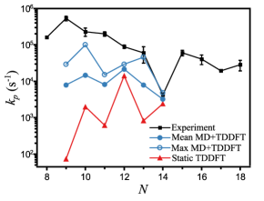
Figure 6: Radiation rate constants of B${}_{N}^{+}$ clusters calculated with the MD+TDDFT analysis (blue circles). Filled and open circles correspond to the mean and the maximum values, respectively. For comparison, the experimental data from Ref. [16] is reproduced in the figure (black squares), together with a calculation using TDDFT on the ground-state geometries (red triangles).

VIII Summary and perspectives

In this work, the role of temperature on the radiative cooling of boron clusters was investigated by means of molecular dynamics simulations in combination with time-dependent density functional theory and high-level ab-initio computations. With a focus on the computational analysis of the B${}_{13}^{+}$ cluster, it was shown that at the effective temperature of 3855 K, estimated from experimental parameters, geometry fluctuations cause significant changes in the electronic structure of the cluster. At several points in the explored geometry, the energy of the low-lying electronic excited states is reduced by a significant amount, with a concomitant exponential increase in the recurrent fluorescence radiation rate. Moreover, the possibility that energy is transferred non-radiatively via IC and IIC was explicitly demonstrated, by large non-adiabatic coupling vectors when the electronic ground and the first electronic excited state cross.

The thermal effects have two important consequences. One is that the rates estimated in this work reduce the discrepancy between theory and experiment significantly, giving a strong indication of the importance of the effect and the modification of the RF values relative to ground state properties.

The second consequence is the occurrence of a significant broadening and redshift of the emission spectrum relative to that of the ground state. The redshift seen in the thermalized spectrum must also be expected to be a general occurrence. The lowest energy geometries tend to be those that maximize the HOMO-LUMO gap for molecules and clusters, and thermal excitation tend to reduce this gap, and hence generally reduce the excited state energies. The tendency is amplified in the emission spectra by the fact that low energy states tend to be more populated by simple phase space arguments. Hence, also this effect will favor a redshift of the spectrum.

There is therefore all reason to believe that the thermal effects described here on the emission rate constants and on the spectral shapes will both be present in other systems that dissipate energy by recurrent fluorescence. It should also be noted that the deformations explored in Fig. 3 imply energy of emitted photons reaching down to close to zero due to level crossings. Measured spectra will therefore show the effect even more strongly than calculated here.

The internal excitation energy was determined as the sum of kinetic energies sampled from the canonical ensemble with the added energy of the S₁ state in the ground state geometry. The choice of using the S₁ state and not the electronic ground state as the initial configuration compensates for the fact that a fraction of the clusters are in electronically excited states, both S₁ and the higher states, and that this excitation energy should be added to the nuclear kinetic energy of 5.61 eV.

It also compensates for the fact that the deformed clusters, that take up most of the phase space, will have nuclear potential energies above those of the harmonic motion of the ground state. It is not possible to know the precise value of this contribution before the entire phase space is sampled or the caloric curve determined experimentally, but an estimate can be obtained by considering the melting enthalpy. The bulk melting point is 2349 K, which is below the temperature here, suggesting that the clusters are liquid, or in the equivalent finite sizes particle phase. The melting enthalpy for bulk is 0.52 eV per atom for bulk. Adding this would more than double the excitation energy. The thermal estimates calculated here are therefore of a very conservative nature, which should be kept in mind when comparing them to the experimental values.

Measurements of recurrent fluorescence spectra is a field in its infancy, with only one spectrum reported so far [13]. The measurements of the spectrum of emitted photons by hot naphthalene molecules in Ref. [13] show a spectrum which is significantly broadened compared to the ground-state absorption case. This experimental observation agrees qualitatively with our calculations shown in Fig. 5.

Measurements of thermal emission spectra of highly excited clusters provide a method to explore the potential energy surfaces of molecules and cluster, which is presently not available with other methods, such as traditional spectroscopy. The results calculated here suggest that such measurements will give significant effects compared to ground state geometry spectra and emission rate constants. The ultimate information will be provided by experiments. The results here tell us that these experiments are worth performing.

IX Acknowledgements

This work is supported by the Research Foundation Flanders (FWO, G.0A05.19N), and the KU Leuven Research Council (project C14/22/103). PF acknowledges the FWO for a senior postdoctoral grant. KH acknowledges support from the National Science Foundation of China with the grant ’NSFC No. 12047501’ and the Ministry of Science and Technology of People’s Republic of China with the 111 Project under Grant No. B20063. T. H. is grateful for the János Bolyai Research Scholarship of the Hungarian Academy of Sciences (grant number BO/00642/21/7).

References

- Hansen and Campbell [1996] K. Hansen and E. Campbell, J. Chem. Phys. 104, 5012 (1996).
- Andersen et al. [1996] J. U. Andersen, C. Brink, P. Hvelplund, M. O. Larsson, B. B. Nielsen, and H. Shen, Phys. Rev. Lett. 77, 3991 (1996).
- Martin et al. [2013] S. Martin, J. Bernard, R. Brédy, B. Concina, C. Joblin, M. Ji, C. Ortega, and L. Chen, Phys. Rev. Lett. 110, 063003 (2013).
- Bernard et al. [2019] J. Bernard, A. Al-Mogeeth, A.-R. Allouche, L. Chen, G. Montagne, and S. Martin, J. Chem. Phys. 150, 054303 (2019).
- Iida et al. [2022] S. Iida, W. Hu, R. Zhang, P. Ferrari, K. Masuhara, H. Tanuma, H. Shiromaru, T. Azuma, and K. Hansen, MNRAS 514, 844 (2022).
- Ferrari et al. [2019] P. Ferrari, E. Janssens, P. Lievens, and K. Hansen, Int. Rev. Phys. Chem. 38, 405 (2019).
- Chernyy et al. [2016] V. Chernyy, R. Logemann, J. Bakker, and A. Kirilyuk, J. Chem. Phys. 145, 024313 (2016).
- Nitzan and Jortner [1972] A. Nitzan and J. Jortner, J. Chem. Phys. 56, 5200 (1972).
- Nitzan and Jortner [1979] A. Nitzan and J. Jortner, J. Chem. Phys. 71, 3524 (1979).
- Leach [1987] S. Leach, in Polycyclic Aromatic Hydrocarbons and Astrophysics, NATO ASI Series, Vol. 191, edited by A. Léger, L. d’Hendecourt, and N. Boccara (1987) pp. 99–127.
- Ebara et al. [2016] Y. Ebara, T. Furukawa, J. Matsumoto, H. Tanuma, T. Azuma, H. Shiromaru, and K. Hansen, Phys. Rev. Lett. 117, 133004 (2016).
- Yoshida et al. [2017] M. Yoshida, T. Furukawa, J. Matsumoto, H. Tanuma, T. Azuma, H. Shiromaru, and K. Hansen, J. Phys.: Conf. Series 875, 012017 (2017).
- Saito et al. [2020] M. Saito, H. Kubota, K. Yamasa, K. Suzuki, T. Majima, and H. Tsuchida, Phys. Rev. A 102, 012820 (2020).
- Hansen et al. [2017] K. Hansen, P. Ferrari, E. Janssens, and P. Lievens, Phys. Rev. A 96, 022511 (2017).
- Peeters et al. [2021] K. Peeters, E. Janssens, K. Hansen, P. Lievens, and P. Ferrari, Phys. Rev. Res. 3, 033225 (2021).
- Ferrari et al. [2018] P. Ferrari, J. Vanbuel, K. Hansen, P. Lievens, E. Janssens, and A. Fielicke, Phys. Rev. A 98, 012501 (2018).
- Fagiani et al. [2017] M. R. Fagiani, X. Song, P. Petkov, S. Debnath, S. Gewinner, W. Schöllkopf, T. Heine, A. Fielicke, and K. R. Asmis, Angew. Chem. Int. Ed. 56, 501 (2017).
- Oger et al. [2007] E. Oger, N. R. Crawford, R. Kelting, P. Weis, M. M. Kappes, and R. Ahlrichs, Angew. Chem. Int. Ed. 46, 8503 (2007).
- Zhai et al. [2014] H.-J. Zhai, Y.-F. Zhao, W.-L. Li, Q. Chen, H. Bai, H.-S. Hu, Z. A. Piazza, W.-J. Tian, H.-G. Lu, Y.-B. Wu, et al., Nat. Chem. 6, 727 (2014).
- Kiran et al. [2009] B. Kiran, G. Gopa Kumar, M. T. Nguyen, A. K. Kandalam, and P. Jena, Inorg. Chem. 48, 9965 (2009).
- Li et al. [2017] W.-L. Li, X. Chen, T. Jian, T.-T. Chen, J. Li, and L.-S. Wang, Nat. Rev. Chem. 1 (2017).
- Arasaki and Takatsuka [2019] Y. Arasaki and K. Takatsuka, J. Chem. Phys. 150, 114101 (2019).
- Hansen [2018] K. Hansen, Statistical physics of nanoparticles in the gas phase (Springer, 2018).
- Kresin and Ovchinnikov [2006] V. V. Kresin and Y. N. Ovchinnikov, Phys. Rev. B 73, 115412 (2006).
- Yanai et al. [2004] T. Yanai, D. P. Tew, and N. C. Handy, Chem. Phys. Lett. 393, 51 (2004).
- Weigend and Ahlrichs [2005] F. Weigend and R. Ahlrichs, Phys. Chem. Chem. Phys. 7, 3297 (2005).
- Shinde [2016] R. Shinde, ACS Omega 1, 578 (2016).
- Gspann [1982] J. Gspann, in Physics of Electronic and Atomic Collisions, edited by S. Datz (1982) pp. 79–96.
- Klots [1987] C. E. Klots, Nature 327, 222 (1987).
- Klots [1991] C. E. Klots, Z. Phys. D 21, 335 (1991).
- Andersen et al. [2001] J. U. Andersen, E. Bonderup, and K. Hansen, J. Chem. Phys. 114, 6518 (2001).
- Casanova and Krylov [2020] D. Casanova and A. I. Krylov, Phys. Chem. Chem. Phys. 22, 4326 (2020).
- Shiozaki et al. [2011] T. Shiozaki, W. Győrffy, P. Celani, and H.-J. Werner, J. Chem. Phys. 135, 081106 (2011).
- Winslow et al. [2020] M. Winslow, W. B. Cross, and D. Robinson, J. Chem. Theory Comput. 16, 3253 (2020).
- Epifanovsky et al. [2021] E. Epifanovsky, A. T. Gilbert, X. Feng, J. Lee, Y. Mao, N. Mardirossian, P. Pokhilko, A. F. White, M. P. Coons, A. L. Dempwolff, et al., J. Chem. Phys. 155, 084801 (2021).
- Shiozaki [2018] T. Shiozaki, WIREs Computational Molecular Science 8, e1331 (2018).
- Ou et al. [2014] Q. Ou, S. Fatehi, E. Alguire, Y. Shao, and J. E. Subotnik, J. Chem. Phys. 141, 024114 (2014).
- Zhang and Herberta [2014] X. Zhang and J. M. Herberta, J. Chem. Phys. 141, 064104 (2014).
- Levine et al. [2006] B. G. Levine, C. Ko, J. Quenneville, and T. J. Martínez, Molecular Physics 104, 1039 (2006).