Fighting Fire with Fire: Avoiding DNN Shortcuts through Priming

Abstract

Across applications spanning supervised classification and sequential control, deep learning has been reported to find “shortcut” solutions that fail catastrophically under minor changes in the data distribution. In this paper, we show empirically that DNNs can be coaxed to avoid poor shortcuts by providing an additional “priming” feature computed from key input features, usually a coarse output estimate. Priming relies on approximate domain knowledge of these task-relevant key input features, which is often easy to obtain in practical settings. For example, one might prioritize recent frames over past frames in a video input for visual imitation learning, or salient foreground over background pixels for image classification. On NICO image classification, MuJoCo continuous control, and CARLA autonomous driving, our priming strategy works significantly better than several popular state-of-the-art approaches for feature selection and data augmentation. We connect these empirical findings to recent theoretical results on DNN optimization, and argue theoretically that priming distracts the optimizer away from poor shortcuts by creating better, simpler shortcuts. Project website: https://sites.google.com/view/icml22-fighting-fire-with-fire/.

1 Introduction

Supervised deep neural networks (DNNs) have led to remarkable achievements across many applications (He et al., 2016; Schrittwieser et al., 2020; Brown et al., 2020). Today’s DNNs learn from a very limited form of supervision, namely, target annotations for each sample in a training dataset. In contrast, when humans learn from annotated examples, they often benefit from richer supervision. When teaching a child to recognize a “zebra” in a zoo enclosure, a parent might draw the child’s attention to the animal and its black-and-white stripes. Without such priming, the learning task is much more poorly defined and there are many equally plausible concepts that the child might learn to identify as “zebra”, such as a zoo enclosure, or any large equine animal including horses and donkeys.

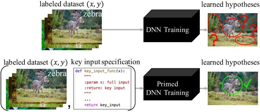
Figure 1: DNNs trained only from label annotation supervision often struggle to disambiguate between competing hypotheses for a target concept, and end up learning “shortcuts”, such as classifying the background as the “zebra”. We propose to expand DNN supervision to include a key input specification function that identifies important portions of the input (such as the foreground object) according to domain knowledge, leading the optimization towards the intended solution.

Indeed, modern DNNs suffer from problems very reminiscent of this confused child. For example, Beery et al. (2018) reports that DNNs trained for animal image recognition successfully classify cows on grass but not on beaches, because they wrongly attribute the label “cow” to the grass. Similarly, autonomous driving DNNs, rather than generating new steering actions in response to changing road observations, commonly learn to copy the previous action, since adjacent actions in training data were almost always very similar (Wen et al., 2020; Bansal et al., 2019; Codevilla et al., 2019). We review more such examples in Section 2. In all these cases, the annotated examples in the training dataset alone cannot sufficiently distinguish the correct solution and prevent the DNN from learning the wrong thing. Following Geirhos et al. (2020), we use the term “shortcut issue” to refer to these phenomena where DNNs fail catastrophically under small distributional shift from training data. How to generalize beyond training distributions is a uniting fundamental question driving many decades-old sub-disciplines of machine learning research, including distributional robustness, domain generalization, zero-shot learning, causality, and invariant learning (Shen et al., 2021; Wang et al., 2021a).

In this work, we argue that many practically encountered ML shortcuts can be circumvented by a simple fix: richer supervision by providing auxiliary “priming” information, beyond merely the target labels. What form should such priming information take? Much like the parent in the introductory example, we propose to exploit commonly available domain knowledge of where in the input the task-relevant information is most likely to lie, for example, the salient foreground for an image classification task, or the most recent observations in autonomous driving. While these “key inputs” do not typically contain all relevant information, and may occasionally not even contain the most relevant information, we find that this is not a problem. It is sufficient that they are likely in many cases to contain key information.

Having decided upon key input-based priming information, how should we provide it to a target DNN learner to help avoid shortcuts? We propose to fight fire with fire by creating a new shortcut that biases the DNN optimization process towards solutions that pay attention to the key inputs. In practice, our “PrimeNet” method consists of first inferring a “priming variable”, typically a coarse estimate of the label, from the key inputs alone. Then, the target DNN which is supplied with this priming variable alongside the full input during training becomes much more likely to avoid shortcuts and “learn the right thing.”

PrimeNet is very simple to implement, can be trained end-to-end, and yields large gains across benchmark tasks for several practical applications ranging from out-of-domain image classification on NICO (He et al., 2021) to imitation learning for controlling robots in MuJoCo (Todorov et al., 2012) and autonomous cars in CARLA (Dosovitskiy et al., 2017). Finally, we argue from recently developed theories of neural network learning that shortcuts are caused by optimization biases that prefer simpler solutions even if they may be trivial or wrong, and that our priming approach works by creating an even simpler yet approximately correct solution within the optimization landscape.

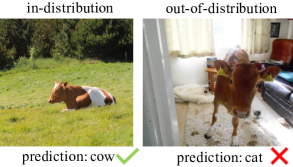
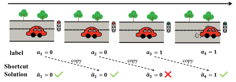
Figure 2: (Left) An example of shortcut learning in image classification in NICO (He et al., 2021). The trained model successfully predicts the “cow” class in the image where the background is grass, while it classifies the cow at home poorly. It indicates that the model recognizes the cow according to the backgrounds rather than the objects. (Right) An example of copycat shortcuts in autonomous driving. The copycat policy learns to cheat by copying from the previous action during training. Therefore, during online testing, when the traffic light turns green, the copycat policy ignores the traffic light and copies the previous action, i.e. staying stationary.

2 Preliminaries: Shortcuts

As introduced above, many surprising error tendencies in deep neural networks arise from strategies that are “superficially successful” (under training circumstances), but fail catastrophically under slightly different circumstances. Following Geirhos et al. (2020), we use the term “shortcut issue” to refer to such errors.

Formally, let $\mathcal{P}_{in}(\bm{x},\bm{y})$ denote a joint probability distribution over $\mathcal{X}$ and $\mathcal{Y}$ from which training data is drawn I.I.D. i.e. $\mathcal{D}_{in}=\{(\bm{x_{i}},\bm{y_{i}})\}_{i=1}^{n}\sim\mathcal{P}_{in}$. Let $\mathcal{P}_{out}(\bm{x},\bm{y})$ denote a different distribution from which the out-of-distribution (O.O.D.) testing set is similarly drawn, i.e. $\mathcal{D}_{out}=\{(\bm{x_{i}},\bm{y_{i}})\}_{i=1}^{m}\sim\mathcal{P}_{out}$. A neural network $f_{\theta}(\cdot)$, parameterized by $\theta$, is trained by SGD with a loss function $l(\cdot,\cdot)$ on the training set $\mathcal{D}_{in}$. Let $\theta^{*}$ denote the intended solution, which can successfully generalize to the O.O.D. distribution, i.e. $\theta^{*}=\arg\min_{\theta}\mathbb{E}_{\mathcal{P}_{in}+\mathcal{P}_{out}}[l(f_{\theta}(\bm{x}),\bm{y})]$. For simplicity, we use $L_{\mathcal{P}}(\theta)$ to denote the population loss of solution $\theta$ on distribution $\mathcal{P}$. Shortcut learning, or the shortcut issue, refers to learning solutions $\theta_{s}$ that perform well under the training distribution, i.e. $L_{\mathcal{P}_{in}}(\theta_{s})\approx L_{\mathcal{P}_{in}}(\theta^{*})$, but generalizes very poorly to O.O.D. data, i.e. $L_{\mathcal{P}_{out}}(\theta_{s})\gg L_{\mathcal{P}_{out}}(\theta^{*})$.

Shortcut issues have been observed in many applications, including computer vision (Beery et al., 2018; Geirhos et al., 2019), NLP (Niven & Kao, 2019; McCoy et al., 2019), imitation learning (Bansal et al., 2019; Codevilla et al., 2019; Wen et al., 2020) and reinforcement learning (Amodei et al., 2016; Zhang et al., 2021a). We highlight image classification and imitation learning shortcuts below, which we will later validate our proposed approach on.

Image classification shortcuts: Consider a DNN-based animal image classifier. Cows in training typically have grass backgrounds, and the classifier may easily learn to rely on grass as an important “shortcut” cue for the “cow” label. Indeed, such a solution would even generalize to in-distribution test data, but fail on in-the-wild distributionally shifted images with cows at home (see Figure 2). Many such shortcuts have recently drawn attention in the image recognition literature (Beery et al., 2018; Rosenfeld et al., 2018; Buolamwini & Gebru, 2018).

Imitation learning shortcuts: Next, consider the task of learning to control a robot or autonomous car from observing expert demonstrations of actions $\bm{a}_{t}$ corresponding to sensory observations (such as camera image streams) $\bm{x}_{t}$ at the same time $t$. “Behavioral cloning” (BC) treats this as supervised learning to regress $\bm{a}_{t}$ from recent observation histories $[\bm{x}_{t-k},\cdots,\bm{x}_{t}]$. In theory, the inclusion of older observations as inputs allows the imitator to compensate for partial observability: for example, a pedestrian occluded in the current camera image from a car dashboard might have been visible earlier. However, the core problem of BC lies in generalizing beyond expert (hence in-distribution) data. Indeed, many previous works (Wen et al., 2020; Muller et al., 2006; de Haan et al., 2019; Bansal et al., 2019; Codevilla et al., 2019; Wen et al., 2021; Ortega et al., 2021) find that BC from observation histories, much like the image classifier above, yields better training and validation losses on expert data, but fails catastrophically when executed on a robot or car. Like the classifier mistaking the grass for the cow, DNN imitators in these situations frequently learn shortcuts that simply copy the last performed action rather than respond to new road images or other observations. This happens because experts usually act smoothly, and adjacent actions in training data are nearly always identical. This “copycat” shortcut can cause curious phenomena like the “inertia problem” (see Figure 2) where cars that once come to rest never move again!

3 Method: Priming DNNs To Avoid Shortcuts

We now describe the core contribution of this paper: an easy-to-implement solution to avoid DNN shortcuts in settings where auxiliary domain knowledge about “key inputs” is available. Section 3.1 sets up our key idea, 3.2 describes the algorithm in detail, 3.3 provides theoretical support, and 3.4 discusses two example applications.

3.1 Motivation

Out-of-distribution generalization for supervised learning is hard, yet humans often manage to generalize far beyond the training data (Geirhos et al., 2018) by exploiting additional knowledge beyond the labels. Recall the example from the introduction of the parent teaching the child to recognize zebras. Besides “labeling” the scene as containing a “zebra”, the parent also points to the animal and its stripes. Without this auxiliary information, it would be a much harder task for the child to acquire the correct concept of a zebra. However, in the common supervised machine learning setup, no such additional information is available; instead, the supervision consists only of labeled examples. We propose to expand this supervision by providing auxiliary knowledge about pertinent “key inputs” to DNNs, to help them to avoid shortcuts and learn the right thing.

To use such auxiliary information well, we draw inspiration from cognitive science. Cognitive scientists have observed a phenomenon called “priming”: exposing humans to one stimulus influences their response to a subsequent stimulus, without conscious guidance or intention (Weingarten et al., 2016; Bargh & Chartrand, 2014). For example, people who were recently exposed to words associated with the elderly (e.g., retirement) begin to walk more slowly than before (Bargh et al., 1996). We propose to prime DNNs during training with the known key inputs to coax them to discover solutions that rely more on that information, matching our knowledge about the correct solution. Next, we will describe this approach, PrimeNet, in more detail.

3.2 PrimeNet

As motivated above, PrimeNet exploits domain knowledge of portions of the full input $x$ that are most likely to contain task-relevant information. While specifying such knowledge for each example would be cumbersome and impractical, we observe that it is often easy to specify this knowledge at a task level. For example, for image classification tasks, the foreground objects, identified perhaps by a generic object detector or salient foreground segmenter, could be specified to the learner as being the most important. In a partially observed sequential control task like vision-based driving, one might specify the most recent frame as likely to contain the most pertinent information. We call these the “key inputs”, denoted as $k(x)$, where the $k(\cdot)$ is a specified process or function that extracts them from the full inputs $x$. The full task specification for PrimeNet thus augments the standard training dataset with this function $k(.)$.

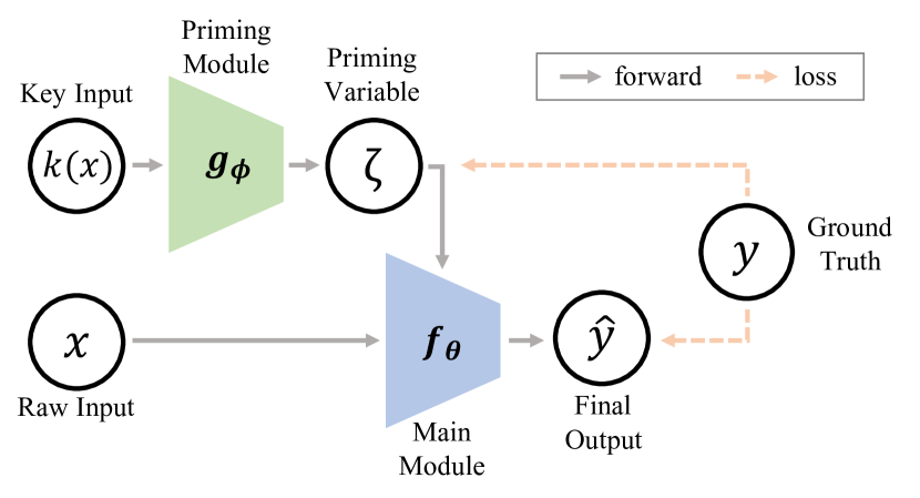
Figure 3: The PrimeNet framework. From the full input $x$, the key input $k(x)$ is extracted using domain knowledge specified through a function $k(.)$. This is then used to “prime” the main module $f_{\theta}$ towards good solutions during training.

As shown in Figure 3, the PrimeNet framework contains two modules: a priming module $g_{\phi}$ and the main module $f_{\theta}$. In the forward pass, the priming module $g_{\phi}$ first computes a coarse estimate $\zeta$ of the target label based on the key inputs $k(x)$, i.e. $\zeta=g_{\phi}(k(x))$. We call this key-input-based coarse estimate $\zeta$ the priming variable. Then, the main module $f_{\theta}$ receives $\zeta$ as input alongside the full input $x$, and produces the final output $\hat{y}=f_{\theta}(x,\zeta)$.

We jointly train the priming module $g_{\phi}$ and main module $f_{\theta}$ end-to-end on the in-distribution training set $\mathcal{D}_{in}={(x_{i},y_{i})}_{i=1}^{n}$ by minimizing standard loss functions $l(\cdot,\cdot)$ as appropriate to the task (e.g., the cross-entropy loss for classification and MSE loss for regression) computed on the outputs of both the priming module (i.e., the priming variable, which we train to be a coarse estimate of the output) and the main module (i.e., the final output).

$$\phi^{*} =\arg\min_{\phi}\frac{1}{n}\sum_{i=1}^{n}l(g_{\phi}(k(x_{i})),y_{i})$$

$$\theta^{*} =\arg\min_{\theta}\frac{1}{n}\sum_{i=1}^{n}l(f_{\theta}(x_{i},\zeta_{i}),y_{i})$$

In our implementation, we concatenate $\zeta$ with intermediate activations in the DNN $f_{\theta}$ and feed them into the following layers together. In this way, the main module is still free to learn a solution that relies on information in the full input that is not available in the key input. This is a necessary property: recall that key inputs merely provide good summaries of task-relevant information, and may not be comprehensive. For example, looking at the background often provides helpful contextual cues when classifying images (Oliva & Torralba, 2007), and remembering older observations may be necessary to account for an occluded pedestrian during driving (Bansal et al., 2019).

This brings us to the question: given that priming does not restrict the hypothesis space and the DNN can still represent the same shortcut solutions as before, how does priming improve DNN training at all, as our results will suggest in Sec 4? We argue that since $\zeta$ itself is a coarse solution for the task, it introduces a simple and desirable shortcut towards low training losses which sets the optimization process for $f_{\theta}$ “on the right track”, away from any catastrophically wrong shortcut solutions. Section 3.3 formalizes this intuition.

3.3 Theoretical Justification

To explain why PrimeNet takes the shortcut from the priming variable $\zeta$ rather than the undesired shortcuts, we derive a property of the neural networks that different inputs guide the optimization to different solutions.

Proposition 3.1.

Consider two functions $h$ and $s$ within the hypothesis space of a neural net, where $h$ is linear with respect to the input. Further, suppose that:

• In the training region, functions $h$ and $s$ are both close to the ground truth.

• In the out-of-distribution testing region, functions $h$ and $s$ are far apart.

Then there exists a training iterate, such that for a neural tangent kernel $f_{NTK}$ trained at such iterate, the following statements (C1-C2) hold with high probability under some mild conditions:

• In the in-distribution region, $f_{NTK}$ reaches small training error.

• In the out-of-distribution region, $f_{NTK}$ approximates $h$ well but stays far from $s$.

We defer the formal statement and proof to Appendix J. Broadly, this proposition states that neural network training, approximated by neural tangent kernels (Jacot et al., 2018), is biased towards solutions that are linear functions of the inputs. In the training region, both the function $h$ which is linear in the input features, as well as a non-linear function $s$ approximate ground truth $y$ well (Assumption A1). Therefore, DNN training may recover either $h$ or $s$ as valid solutions. However, 3.1 demonstrates that in the O.O.D. region, neural networks indeed prefer the simple function $h$, which is linear in the input features. The proof starts from Hu et al. (2020b), which shows that neural networks during early training approximate a linear model, and we further extend the conclusion to the O.O.D. region, providing theoretical justification for using priming to solve shortcut problem (see below).

Remark. What does Proposition 3.1 say about why PrimeNet works? If the input of the main module $f_{\theta}$ is $[x,\zeta]$, then the DNN will prefer simple functions (such as linear functions) of $x$ and $\zeta$ even in the O.O.D. region, and changes in $\zeta$ may significantly change this preference, even though $\zeta$ is computed from the full input $x$ and therefore cannot introduce any new information. Thus, setting $\zeta$ to represent coarse output estimates based on key input domain knowledge encourages the DNN to find solutions that also rely on the key input.

3.4 Applying PrimeNet

Recall the two shortcut issue examples from Section 2. For the image classification problem, shortcuts are caused by background distractions, and we consequently set the key input function $k(.)$ to be an image patch crop from unsupervised saliency detection (Qin et al., 2019). This provides a background-free image patch for priming without the risk of introducing shortcuts into the extraction of the priming variable $\zeta$ itself. In the imitation setting, shortcuts are caused by the implicit previous action in the historical observations. To remove this shortcut, we propose to use the most recent frame as the priming input, i.e. $k(x)=x_{t}$. Once again, this might lose some information, but it can serve as the basis for a coarse action estimate that is free from shortcuts. See Section 4 and Appendix G and Appendix H for more details.

4 Experiments

We conduct experiments on three sets of tasks: a toy regression experiment, an image classification task and two behavioral cloning tasks on autonomous driving and robotic control to verify our arguments and the proposed method. The toy experiment is to validate the Proposition 3.1. The realistic image classification and behavioral cloning tasks are designed to verify that our method can resolve shortcut issues and evaluate it against previous state-of-art methods. Finally, we conduct ablation and analysis studies on these two tasks to study our method more closely.

Table 1: RMSEs for the 1-D regression experiment.

	I.I.D.		O.O.D.
$\zeta$ value	$f_{1}$	$f_{2}$	$f_{1}$	$f_{2}$
0	0.101	0.121	18.126	8.838
$x^{4}$	0.100	0.122	9.062	0.258
$x^{5}$	0.100	0.122	0.243	9.075

4.1 One-Dimensional Regression

We design a toy 1-D regression experiment on synthetic data to empirically validate Proposition 3.1. To construct a scenario with multiple local optimal solutions on the training set and with the challenge of O.O.D. generalization, we design two functions: $f_{1}(x)=1.5x^{5}+2x+\epsilon$ and $f_{2}(x)=1.5x^{4}+2x+\epsilon$, where $\epsilon\sim N(0,0.1)$ is an additive Gaussian noise. These two functions are close to each other in the training region $[0,1]$, and significantly different in the testing region $[1,2]$. We uniformly sample 1000 training pairs $(x_{i},f_{1}(x_{i}))$ in the training region $x_{i}\in U(0,1)$. We train a two-layer MLP to fit the training data with the input $[x,\zeta]$, where $[\cdot,\cdot]$ means concatenation operation and $\zeta$ is the priming variable. We train three models with $\zeta$ equal to 0, $x^{4}$ or $x^{5}$ respectively. We test each trained model on two testing regions, i.e. the in-distribution region $[0,1]$ and O.O.D. region $[1,2]$, and with two reference functions as priming variables $\zeta$, i.e. $f_{1}$ and $f_{2}$. We want to study which solution the MLP will converge to, when given different $\zeta$. The accuracy on the O.O.D. region will indicate what function the neural network has learned during training.

Table 1 reports the RMSE value of the trained models against $f_{1}$ and $f_{2}$ on in-distribution and out-of-distribution testing sets. All models fit the training data perfectly regardless of the choice of priming variable $\zeta$, and the RMSEs on $f_{1}$ and $f_{2}$ are close in the in-distribution region $[0,1]$ because the two functions are very similar in this range. When testing the models in the O.O.D. region $[1,2]$, the model fits $f_{2}$ better when primed on $x^{4}$, and fits $f_{1}$ better if primed on $x^{5}$. This is true even though the labels in the training data were generated by $f_{1}$. This shows that the priming variable $\zeta$ can significantly influence DNN training towards simpler functions of $[\zeta,x]$, consistent with Proposition 3.1. We visualize the learned functions in Appendix A.

4.2 Image Classification

O.O.D. image classification is a challenging task that has attracted attention in computer vision in recent years (Arjovsky et al., 2019; Krueger et al., 2021b; Xu et al., 2021; Wang et al., 2021b). We evaluate PrimeNet on an O.O.D. image classification benchmark.

NICO (He et al., 2021) is an image classification dataset designed for O.O.D. settings. In total, it contains 19 classes, 188 contexts and nearly 25,000 images. Besides the object label (cat, dog, cow, etc.), each of the images is also labeled with a context label (at home, on beach, on grass, etc.). Thus, it is convenient to design the distribution of data by adjusting the proportions of specific contexts for training and testing images. We use the animal subset of NICO with 10 categories, and each class has 10 contexts. Following Wang et al. (2021b), we construct a challenging O.O.D. setting: 1) the training dataset has only 7 contexts for each object category and the testing dataset has all the 10 contexts to evaluate the zero-shot generalization capability of the models (see the examples in Figure 2 (left)); 2) the context labels in the training set are in long-tailed distribution, which makes it more difficult to train an unbiased classifier. We employ ResNet-18 (He et al., 2016) as the backbone network for all the methods. For our method, we use a weight shared ResNet-18 as $g_{\phi}$ and $f_{\theta},$ and utilize the unsupervised saliency detection model BASNet (Qin et al., 2019) to crop the salient areas of the full images as $k(x)$. See Appendix G for the architecture, implementation and training details.

4.2.1 Baselines

For image classification, we extensively compare PrimeNet with four classes of methods: a set of vanilla baselines designed by us, and three sets of methods to improve generalization using debias, image augmentation and intervention techniques.

Vanilla baselines. We design three vanilla baselines with the ResNet18 model: 1) Vanilla ResNet18 (He et al., 2016): directly adopting the ResNet18 model to classify the images; 2) Key-Input-Only baseline: using the key input $k(x)$ as the input of ResNet18; 3) Average-Ensemble baseline: training ResNet18 on an expanded dataset containing the original images $x$ as well as the extracted key input regions $k(x)$, and then averaging the output logits for $x$ and $k(x)$ for classification during testing.

Debias methods. We compare our method with two SOTA debias methods: RUBi (Cadene et al., 2019), ReBias (Bahng et al., 2020) and StableNet (Zhang et al., 2021b). RUBi learns a biased model with the biased dataset and then trains an unbiased model by re-weighting according to the predicted logits of the biased model. ReBias firstly train a small biased model with the biased dataset and regularizes the main model to be statistically independent from it. StableNet removes spurious correlations by reweighting training samples to get rid of feature dependencies.

Data augmentation methods. We adopt two commonly used data augmentation methods, Mixup (Zhang et al., 2017) and Cutout (DeVries & Taylor, 2017). Mixup linearly interpolates the inputs and labels of two random training samples, thus extending the training distribution. Cutout randomly masks out a square patch on the full image to avoid overfitting to the contexts.

Causal inference methods. We also compare to two SOTA causal methods: IRM (Arjovsky et al., 2019) and Caam (Wang et al., 2021b). IRM proposes to learn an invariant representation which gets optimal classification performance across different environments (contexts) to remove the effect of the spurious shortcut correlations. It requires the environment labels. Caam improves IRM by automatically getting the environment partitions in the training set and utilizes IRM to boost the performance.

4.2.2 Results

Table 3 shows the classification accuracy on test sets of all the methods. PrimeNet achieves significantly better performance than the baselines across all the settings. PrimeNet (ours) and CAAM significantly improve the in-domain accuracy (as well as OOD), and ours is better than CAAM on both. We believe this happens because NICO has relatively small training datasets with incomplete coverage of the training distribution, so even in-domain generalization can sometimes benefit from removing shortcuts. Other methods (e.g. Average-Ensemble and StableNet) improve the OOD generalization while harming the in-domain performance.

Table 2: Image classification accuracies on the NICO dataset. Baseline scores from Wang et al. (2021b). “-” means the value is neither reported in Wang et al. (2021b) nor reproduced by us because we do not have the source codes.

Method	in-domain test	ood test
vanilla ResNet18	66.11	42.61
key-input-only	62.78	47.54
average-ensemble	63.33	47.69
Rubi (Cadene et al., 2019)	-	44.37
ReBias (Bahng et al., 2020)	-	45.23
CutOut (DeVries & Taylor, 2017)	-	43.77
MixUp (Zhang et al., 2017)	62.78	41.46
IRM (Arjovsky et al., 2019)	-	41.46
StableNet (Zhang et al., 2021b)	63.33	43.62
Caam (Wang et al., 2021b)	70.00	46.62
PrimeNet (ours)	71.11	49.00

As for OOD performance, compared to vanilla ResNet18, PrimeNet improves accuracy by more than 6%, illustrating that our method successfully alleviates the shortcuts from the background contexts, and thus gets better generalization performance. We note that although the Key-Input-Only method already performs better than previous methods, our PrimeNet further improves on top of it, showing that PrimeNet manages to effectively integrate information from non-key areas, unlike Key-Input-Only. Compared with the SOTAs of debias (Rubi, ReBias and StableNet), data augmentation (Cutout and Mixup) and intervention (IRM and Caam) methods, our method introduces an alternative inductive bias, i.e. key input from unsupervised saliency detection. This does not require any additional supervision, relying only on the domain knowledge that foreground objects contain the most pertinent information for this task. This validates that saliency-based key input priming is an effective and practical inductive bias for resolving image classification shortcuts.

4.3 Behavioral Cloning For Imitation

The O.O.D. generalization problem is the main bottleneck of behavioral cloning, which is widely recognized over many decades (Muller et al., 2006; Ross et al., 2011; Bansal et al., 2019; Wen et al., 2020; Spencer et al., 2021). We evaluate PrimeNet on two imitation learning tasks.

CARLA. CARLA is a photorealistic urban autonomous driving simulator (Dosovitskiy et al., 2017), and it is a commonly adopted testbed for imitation learning (Codevilla et al., 2018, 2019; Chen et al., 2020; Wen et al., 2021; Prakash et al., 2021). We use the CARLA100 dataset to train all methods and evaluate them in the Nocrash benchmark (Codevilla et al., 2019). Following Wen et al. (2021), the POMDP observations don’t include the vehicle speed, and imitation learners can instead use past video frames to prescribe driving actions. We train all the methods three times from different random initializations to account for variance (Codevilla et al., 2019). We use CILRS (Codevilla et al., 2019) as the backbone, set the length of input observation history to $7$, and stack the sequential frames along the channel dimension as the model input as in Bansal et al. (2019); Wen et al. (2021). We report the mean and standard deviation of two metrics: %success and #timeout. %success is the number of episodes that are fully completed out of 100 pre-designed evaluation routes. #timeout counts the times that the agent fails to reach the destination despite no collision within the specified time. Timeout is usually caused by unsuccessful starts, wrong routes or traffic jams. We report more evaluation metrics, and implementation details in Appendices C and H.

MuJoCo. We evaluate our method in three standard OpenAI Gym MuJoCo continuous control environments: Hopper, Ant and HalfCheetah. We generate expert data from a PPO (Schulman et al., 2017) policy (10k samples for Ant and Walker2D, and 20k for Hopper). To simulate partial observations, we add Gaussian noise ${N}(0,\sigma^{2})$ with $\sigma=0.2$ to joint velocities. We stack 2 frames to form the observation history, and use 2-layer MLPs as policy network backbones. We train all methods with 3 random initializations and report mean and standard deviation of rewards. See Appendix I for network architecture and training details.

4.3.1 Baselines

For BC, we compare against three groups of methods:

Vanilla baselines. We retain the vanilla baselines from image classification, training them for BC. Note that vanilla-BC and key-input-only corresponds to behavioral cloning from observation histories and single observation (BC-OH and BC-SO respectively) as studied in prior works (Wen et al., 2020, 2021). We use CILRS (Codevilla et al., 2019) and two-layer MLPs as the policy network backbone in place of ResNet18 for CARLA and MuJoCo respectively.

Previous methods tackling BC shortcuts. We compare PrimeNet with three previous solutions to the shortcuts in BC: fighting copycat agents (FCA) (Wen et al., 2020), KeyFrame (Wen et al., 2021) and History-Dropout (Bansal et al., 2019). FCA proposes to resolve the shortcut issue with adversarial training, which removes information about the previous action $a_{t-1}$. KeyFrame tackles the shortcut in BC from an optimization perspective: it up-weights the datapoints at action change-points, which is defined as an action prediction module’s failure timesteps. History-Dropout introduced a dropout on the observation history to randomly erase the channels of historical frames.

Online “upper bound” solution. We also compare with an online imitation learning method, DAGGER (Ross et al., 2011). DAGGER is a widely used method to mitigate domain shift issues in imitation learning, but requires online environmental interaction with a queryable expert. We note that our method does not require the online expert, and thus DAGGER is an “upper bound”, rather than a baseline. In our experiments, DAGGER uses 150k supervised interaction steps for CARLA and 8k for MuJoCo.

4.3.2 Results

Table 3: Behavioral cloning results on CARLA and MuJoCo.

	carla results		mujoco rewards
method	%success	#timeout	hopper	ant	halfcheetah
vanilla bc	34.1 $\pm$ 7.5	36.1 $\pm$ 14.5	628 $\pm$ 99	2922 $\pm$ 1266	639 $\pm$ 121
key-input-only	13.1 $\pm$ 1.8	11.1 $\pm$ 2.9	589 $\pm$ 94	4198 $\pm$ 433	489 $\pm$ 77
average-ensemble	41.7 $\pm$ 3.1	15.0 $\pm$ 0.8	504 $\pm$ 47	4659 $\pm$ 396	729 $\pm$ 50
PrimeNet (ours)	49.3 $\pm$ 3.6	12.0 $\pm$ 1.9	1124 $\pm$ 135	4798 $\pm$ 304	1448 $\pm$ 74
fca (Wen et al., 2020)	31.2 $\pm$ 5.2	35.3 $\pm$ 9.6	831 $\pm$ 108	3727 $\pm$ 926	1148 $\pm$ 81
Keyframe (Wen et al., 2021)	41.9 $\pm$ 6.2	24.8 $\pm$ 7.9	696 $\pm$ 28	2930 $\pm$ 1321	1062 $\pm$ 127
history-dropout (Bansal et al., 2019)	35.6 $\pm$ 3.5	20.3 $\pm$ 5.6	539 $\pm$ 33	4069 $\pm$ 517	1215 $\pm$ 70
dagger (Ross et al., 2011)	42.7 $\pm$ 5.7	23.0 $\pm$ 7.1	2383 $\pm$ 294	4097$\pm$ 418	1842 $\pm$ 10

CARLA. Table 3 shows results on the hardest benchmark with the densest traffic, Nocrash-Dense. Key-input-only performs poorly, and is even worse than vanilla BC on %success. It sees only the last frame and has no way to judge its own speed, so it most commonly fails by accelerating at all times on straight roads, resulting in speeding and collisions. Vanilla BC has access to past frames, but suffers from very high #timeout rates due to starting problems: once the car stops, say, at a traffic light, vanilla BC often remains stationary until timeout. This high #timeout is known to be a typical copycat shortcut symptom (Wen et al., 2020, 2021; Bansal et al., 2019) for BC from observation histories.

It is thus especially interesting that PrimeNet reduces the #timeout to $12.0$, very close to key-input-only. PrimeNet also outperforms all baselines on %success, remarkably even including the “upper bound” DAGGER. Appendix C shows results on Nocrash-Empty and Nocrash-Regular.

MuJoCo. Table 3 also shows results on Hopper, Ant, and HalfCheetah. Here, vanilla BC only performs slightly better than key-input-only on Hopper and HalfCheetah, and does worse than key-input-only on Ant, due to the copycat shortcut. PrimeNet beats out all baselines, including prior approaches addressing BC shortcuts (FCA, KeyFrame and History-Dropout), in all 3 environments. The upper bound DAGGER approach does significantly better than all methods on Hopper and Half-Cheetah, but Key-Input-Only and PrimeNet beat it on Ant.

4.4 Ablation Study

Table 4: The ablation study results on NICO and CARLA.

	NICO	CARLA
method	test acc.	%success	#timeout
PrimeNet (ours)	49.00	49.3	12.0
ResNet-early-feature as $\zeta$	45.00	39.8	28.1
ResNet-late-feature as $\zeta$	48.62	44.8	15.9
No-Key-Input	43.92	37.1	28.9
$k(x)$-for-Both-Modules	47.92	13.8	11.9

We now study PrimeNet in more detail through ablations.

Priming variable selection. Should the priming variable be the output of priming module $g_{\phi}$, as we have been using, or should it rather be an intermediate representation of the key input from $g_{\phi}$? We evaluate an early/shallow (layer2) and a late/deep feature (last layer) from $g_{\phi}$ (in place of the output) as the priming variable to be fed to the main module. Table 4 shows a clear trend: shallower priming variables are always worse, and the output from $g_{\phi}$ performs best. This suggests that shallower features do not as effectively create good priming shortcuts to prevent bad shortcut learning.

Role of key inputs. In Table 4, we report the results of using our architecture with no key input (with $x$ as the input to both trunks), and an architecture with key input $k(x)$ for both modules. Under both conditions, the performance on both NICO and CARLA becomes worse, with no-key-input even close to the vanilla baseline. This indicates that the specific design choices of PrimeNet are important to help avoid shortcuts. Appendix D shows more ablations.

4.5 Analysis

We use the activation map (Muhammad & Yeasin, 2020) of ResNet Layer3 on CARLA to illustrate the visual cues that are attended to by different models. As shown in Figure 4, key-input-only model and our PrimeNet correctly notice the red traffic light and the pedestrian. In contrast, vanilla BC shows symptoms of the shortcut problem, paying little attention to the pedestrian and ignoring the traffic light, eventually causing traffic light violation and collision. PrimeNet thus learns to attend to the correct cues in the observations, rather than rely on shortcuts. The activation maps of NICO experiment can be found in Appendx B. Appendix E has more analyses.

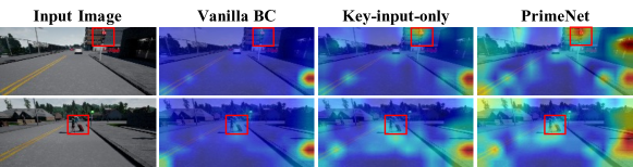
Figure 4: The activation maps are extracted from the Layer3 in the ResNet34 of the perception module of the backbone CILRS (Codevilla et al., 2019). There are two scenarios of slowing down in front of a red traffic light (top) and a pedestrian (bottom). The red areas in the red boxes are where the policies should pay attention to. We can see that the key-input-only model and our PrimeNet correctly focus on the traffic light and the pedestrian while the vanilla BC pays much less attention to the pedestrian and even ignores the traffic light.

5 Related Work

Shortcut Issues in Machine Learning O.O.D. generalization (Krueger et al., 2021a; Hendrycks et al., 2020) has a long history of research in machine learning under names including “learning under covariate shift” (Bickel et al., 2009; Cao et al., 2011), “simplicity bias” (Shah et al., 2020; Xu et al., 2019; Hu et al., 2020c), “anti-causal learning” (Schölkopf et al., 2012), and “shortcuts” (Geirhos et al., 2020). Unlike prior solutions requiring collecting more data (de Haan et al., 2019), utilizing the biased model (Clark et al., 2019; He et al., 2019), obtaining extra labels (Arjovsky et al., 2019; Ahuja et al., 2020; Krueger et al., 2021a), or making assumptions on the distribution (Duchi & Namkoong, 2021; Delage & Ye, 2010; Sagawa et al., 2019), we guide the optimization with additional domain knowledge about key inputs, and show that this helps reduce shortcut issues.

Shortcuts in Image Classification. Specific to image classification, many researchers have observed O.O.D. problems (Bahng et al., 2020; He et al., 2021; Arjovsky et al., 2019), and proposed to alleviate them by de-biasing (Cadene et al., 2019; Bahng et al., 2020; Zhang et al., 2021b), data augmentation (Zhang et al., 2017; DeVries & Taylor, 2017; Xu et al., 2021) and causal intervention (Arjovsky et al., 2019; Ahuja et al., 2020; Krueger et al., 2021b; Wang et al., 2021b) methods. In contrast, we propose to obtain the most task-relevant region in the image by unsupervised models to distract the optimization away from undesired shortcuts and show O.O.D. generalization.

Shortcuts in Behavior Cloning Behavior cloning (BC) suffers from O.O.D. issues because of the mismatch between the offline training distribution and online testing distribution (Muller et al., 2006; Ross et al., 2011; Bansal et al., 2019). In our experiments, we focus on resolving a specific aspect of distributional shift in BC from observation histories – the “copycat” shortcut (Wen et al., 2020). Prior attempts to solve this include removing historical frames (Muller et al., 2006), causal discovery (de Haan et al., 2019), history dropout (Bansal et al., 2019), speed prediction regularization (Codevilla et al., 2019), data re-weighting (Wen et al., 2021), and causal intervention (Ortega et al., 2021). Instead, we focus on resolving the copycat shortcut by priming the policy with information from the most recent observation alone, achieving state-of-the-art performance.

6 Conclusion and Discussion

Summary: In this paper, we propose PrimeNet, a simple and effective approach to resolve the shortcut issue in settings that permit domain knowledge of important inputs. PrimeNet is supported by recent theories on DNN training. On image classification and behavioral cloning tasks, our method outperforms the existing methods and significantly alleviates the shortcut issue to generalize beyond the training distribution.

Limitation: PrimeNet’s gains come from the extra supervision in the form of correct/useful key input information. Though such domain knowledge is often easy to provide, it is indeed possible for poorly defined key inputs to hurt performance, which is a limitation of our method. Future work to address this, such as by automatically discovering key inputs from data, may make our method robust to such mis-specification.

7 Acknowledgements

We thank the anonymous reviewers for their helpful feedback. This work is supported by the Ministry of Science and Technology of the People’s Republic of China, the 2030 Innovation Megaprojects “Program on New Generation Artificial Intelligence” (Grant No. 2021AAA0150000), and a grant from the Guoqiang Institute, Tsinghua University.

Appendix A The learned function in the toy experiment

To verify how the priming variable $\zeta$ affects the final solution of the neural network in the toy regression experiment, we plot the curves of $\hat{y}$ vs. $x$ when providing different values of $\zeta$, 0 (no priming input) or $x^{4}$ or $x^{5}$. We plot the learned curves in different training epochs. As shown in Figure 5, we can see that in the left subfigure, the model without priming input cannot learn an accurate solution and performs poorly in the out-of-distribution region. The middle and right subfigures show that if provided different priming variables, the neural networks will converge to different solutions. Furthermore, the final solution is close to $\zeta$, i.e. the priming variable guides the training of the NNs, which provides an empirical evidence for Proposition 3.1.

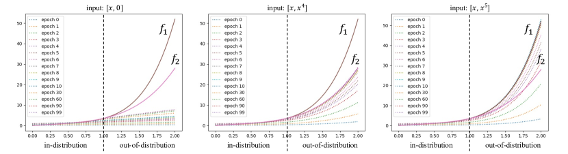
Figure 5: The curve of learned function of the neural network during training. The two solid lines are the ground truth curves of $f_{1}=1.5x^{5}+2x$ and $f_{2}=1.5x^{4}+2x$ respectively (we remove the additive Gaussian noise $\epsilon$ when plotting). The dashed lines are the functions learned by the MLP in different training epochs. We can see that if given different values of priming variable $\zeta$, the solution of the neural network will converge to different regions which are close to $\zeta$.

Appendix B Visualization results of NICO

Similar to Figure 4 for CARLA driving, Figure 6 shows activation maps for NICO. Vanilla ResNet18 learns a background shortcut and makes the wrong prediction, while PrimeNet correctly focuses on the discriminative foreground objects of the images.

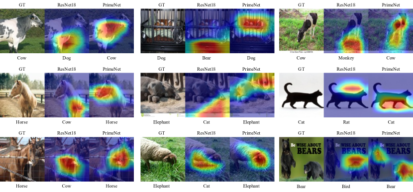
Figure 6: The activation maps of NICO classification model.

Appendix C The detailed imitation results on CARLA Nocrash

The full results on Nocrash-Empty, Nocrash-Regular and Nocrash-Dense are shown in Table 5, Table 6 and Table 7. We can see that our method performs significantly better than vanilla BC, key-input-only and other baselines. Our method gets highest %success and lowest #timeout, indicating that the shortcut in driving scenario, i.e. copycat problem, has been significantly alleviated.

Table 5: CARLA Nocrash-Empty results.

Method	%success ($\uparrow$)	%progress ($\uparrow$)	#collision ($\downarrow$)	#timeout ($\downarrow$)
vanilla bc	78.4 $\pm$ 11.6	83.2 $\pm$ 12.0	1.6 $\pm$ 1.8	20.0 $\pm$ 12.7
key-input-only	44.9 $\pm$ 6.7	68.1 $\pm$ 5.3	39.7 $\pm$ 11.2	15.4 $\pm$ 5.4
average-ensemble	84.1 $\pm$ 5.0	88.8 $\pm$ 2.8	1.0 $\pm$ 0.8	14.9 $\pm$ 5.3
ours	89.8 $\pm$ 1.4	92.6 $\pm$ 0.8	1.6 $\pm$ 1.3	8.6 $\pm$ 1.3
fca	70.4 $\pm$ 7.6	86.1 $\pm$ 6.4	3.6 $\pm$ 1.8	26.0 $\pm$ 7.3
Keyframe	90.1 $\pm$ 5.7	92.9 $\pm$ 2.3	0.6 $\pm$ 0.7	9.3 $\pm$ 5.4
history-dropout	85.1 $\pm$ 3.7	93.6 $\pm$ 2.6	2.2 $\pm$ 1.3	12.7 $\pm$ 4.2
dagger 150k	83.2 $\pm$ 9.4	90.4 $\pm$ 6.0	1.8 $\pm$ 0.9	15.0 $\pm$ 9.4

Table 6: CARLA Nocrash-Regular results.

Method	%success ($\uparrow$)	%progress ($\uparrow$)	#collision ($\downarrow$)	#timeout ($\downarrow$)
vanilla bc	67.1 $\pm$ 10.8	76.5 $\pm$ 10.2	11.1 $\pm$ 3.1	21.9 $\pm$ 12.7
key-input-only	37.6 $\pm$ 6.1	61.2 $\pm$ 4.3	53.0 $\pm$ 7.9	10.2 $\pm$ 3.1
average-ensemble	75.8 $\pm$ 3.6	84.4 $\pm$ 2.0	12.1 $\pm$ 3.0	12.4 $\pm$ 4.5
ours	81.1 $\pm$ 4.0	88.1 $\pm$ 2.6	11.9 $\pm$ 3.3	7.2 $\pm$ 2.8
fca	58.0 $\pm$ 8.0	78.5 $\pm$ 7.1	14.7 $\pm$ 3.3	27.3 $\pm$ 8.8
Keyframe	74.4 $\pm$ 7.3	83.2 $\pm$ 3.4	13.8 $\pm$ 2.7	11.9 $\pm$ 5.8
history-dropout	70.1 $\pm$ 4.0	82.1 $\pm$ 2.2	18.3 $\pm$ 5.2	12.2 $\pm$ 4.4
dagger 150k	69.7 $\pm$ 8.4	80.6 $\pm$ 6.0	14.8 $\pm$ 2.9	15.9 $\pm$ 8.5

Table 7: CARLA Nocrash-Dense results.

Method	%success ($\uparrow$)	%progress ($\uparrow$)	#collision ($\downarrow$)	#timeout ($\downarrow$)
vanilla bc	34.1 $\pm$ 7.5	62.2 $\pm$ 9.4	30.2 $\pm$ 7.9	36.1 $\pm$ 14.5
key-input-only	13.1 $\pm$ 1.8	40.8 $\pm$ 3.0	76.4 $\pm$ 3.5	11.1 $\pm$ 2.9
average-ensemble	41.7 $\pm$ 3.1	71.5 $\pm$ 3.2	43.7 $\pm$ 4.0	15.0 $\pm$ 0.8
PrimeNet (ours)	49.3 $\pm$ 3.6	75.0 $\pm$ 1.6	39.4 $\pm$ 5.0	12.0 $\pm$ 1.9
fca (Wen et al., 2020)	31.2 $\pm$ 5.2	66.5 $\pm$ 4.1	34.4 $\pm$ 8.1	35.3 $\pm$ 9.6
Keyframe (Wen et al., 2021)	41.9 $\pm$ 6.2	70.2 $\pm$ 4.0	33.9 $\pm$ 6.6	24.8 $\pm$ 7.9
history-dropout (Bansal et al., 2019)	35.6 $\pm$ 3.5	67.0 $\pm$ 2.7	45.3 $\pm$ 3.5	20.3 $\pm$ 5.6
dagger 150k (Ross et al., 2011)	42.7 $\pm$ 5.7	71.3 $\pm$ 1.9	35.0 $\pm$ 3.6	23.0 $\pm$ 7.1

Appendix D More ablation studies

We conduct more ablation studies on CARLA and the detailed results are shown in Table 8.

Table 8: CARLA ablation study results.

Method	%success ($\uparrow$)	%progress ($\uparrow$)	#collision ($\downarrow$)	#timeout ($\downarrow$)
PrimeNet (ours)	49.3 $\pm$ 3.6	75.0 $\pm$ 1.6	39.4 $\pm$ 5.0	12.0 $\pm$ 1.9
early-fusion	51.4 $\pm$ 4.0	75.9 $\pm$ 2.1	37.4 $\pm$ 5.1	12.7 $\pm$ 2.6
middle-fusion	49.6 $\pm$ 1.7	74.8 $\pm$ 1.9	37.3 $\pm$ 4.0	13.3 $\pm$ 3.0
resnet layer2 as $\zeta$	39.8 $\pm$ 4.0	69.4 $\pm$ 1.5	32.6 $\pm$ 1.5	28.1 $\pm$ 4.4
resnet avg-pool as $\zeta$	44.8 $\pm$ 5.2	71.9 $\pm$ 4.7	40.0 $\pm$ 5.7	15.9 $\pm$ 3.4
$g_{\phi}(x)$ and $f_{\theta}(x,\zeta)$	37.1 $\pm$ 3.4	66.9 $\pm$ 2.8	34.1 $\pm$ 3.4	28.9 $\pm$ 6.0
$g_{\phi}(x)$ and $f_{\theta}(k(x),\zeta)$	31.7 $\pm$ 5.7	62.2 $\pm$ 6.1	28.3 $\pm$ 9.0	40.0 $\pm$ 14.7
$g_{\phi}(k(x))$ and $f_{\theta}(k(x),\zeta)$	13.8 $\pm$ 2.4	41.8 $\pm$ 4.5	74.9 $\pm$ 3.2	11.9 $\pm$ 2.6
w/o stop-gradient	44.4 $\pm$ 5.5	71.4 $\pm$ 3.0	39.2 $\pm$ 4.7	17.1 $\pm$ 2.1
w/o end-to-end	47.3 $\pm$ 3.8	71.2 $\pm$ 1.2	43.4 $\pm$ 5.5	9.8 $\pm$ 3.1

Different fusion stages. We can see that given the priming variable $\zeta$, it makes no difference where to inject it into $f_{\theta}$ (%success ranges from $49.3$ to $51.4$ and other metrics are similar too), indicating that $\zeta$ provides a simpler shortcut than inferring and copying the previous action from the observation history. Wherever we inject $\zeta$, the neural network prefers to adopt it directly as the decision rather than expending greater effort to take the copycat shortcut.

Stop-gradient. Moreover, we find that the agent performs worse if we remove stop-gradient (%success drops from 49.3 to 44.4), which is mainly due to timeout (increasing from 12.0 to 17.1). The increasing #timeout shows that our method without stop-gradient still suffers from the shortcuts due to redundant information leakage during back-propagation.

Two-stage training. And training $g_{\phi}$ and $f_{\theta}$ stage-by-stage, the performance also deteriorates (%success drops from 49.3 to 47.3). We can see that its #timeout is even fewer than ours but it gets a significantly higher #collision (#collision increases from 39.4 to 43.4), indicating that the agent trained stage-by-stage behaves more like key-input-only model, i.e. suffering from less copycat but failing to brake in time. We hypothesize that if we use a pretrained priming module $g_{\phi}$ at the beginning of $f_{\theta}$ training, $f_{\theta}$ will prefer to just copy the $\zeta$ as its output rather than learn from scratch to take accurate actions according to both the priming variable and observation history, which can also be viewed as overly relying on the ”simpler” solution.

Appendix E More Analysis Experiments

Then, because there are two inputs of main module $f_{\theta}$, we investigate the effect of the priming variable $\zeta$ and the input observation history $x$ on $f_{\theta}$.

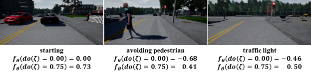
Figure 7: Examples of scenarios with high effects of the priming variable $\zeta$. The $f_{\theta}(do(\zeta)=0.00/0.75)$ means that we manually set the value of $\zeta$ to 0.00 and 0.75 respectively, fix the input $x$ and then get the output of the $f_{\theta}$. The larger the difference between $f_{\theta}(do(\zeta)=0.00)$ and $f_{\theta}(do(\zeta)=0.75)$, the stronger the effect of $\zeta$.

The effect of the priming variable $\zeta$. To study the effect of the priming variable in our model, we set the value of $\zeta$ manually while keeping all other factors the same. This process is similar to the intervention technique in causal inference literature (Rubin, 1974, 1978; Pearl, 1995), so we borrow the do-calculus $do(\zeta)$ from causal inference to denote this operation. For easier interpretability, we only modify the acceleration dimension, i.e. setting throttle to 0 and 0.75 (the highest value in expert demonstrations), which can be denoted as $do(\zeta)=0/0.75$. The effect of $\zeta$ can be defined by $\text{Effect}=|f_{\theta}(do(\zeta)=0)-f_{\theta}(do(\zeta)=0.75)|$, where we omit another input variable $x$ for simplicity. Through studying the effect of $\zeta$ along the trajectories, we find that $\zeta$ tends to have a very high effect at some critical moments such as the examples in Figure 7, illustrating the important guidance effect of $\zeta$ in PrimeNet. Especially, the effect of $\zeta_{t}$ is high when the car is starting, but it decreases after the car is started because at this time it is necessary to refine its actions according to observation history, which is what we expected.

The effect of the input observation history $x$. Similarly, to study the effect of the input observation history $x$, we intervene it by repeating the current frame $H$ times, i.e. $do(x)=\left[o_{t},o_{t},\cdots\right]$ which creates counterfactual stationary cases, i.e. the previous action is 0. Recall the example in Section 2, to investigate what factors the agents use to determine whether to move forward or stop, we count the percentage of model outputs that change from accelerating to stop after we intervene on the input sequence, i.e.

$$\frac{N(\text{speed}>0,f_{\theta}(x)>0,f_{\theta}(do(x))=0)}{N(\text{speed}>0,f_{\theta}(x)>0)}$$

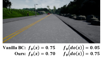
Figure 8: An example of intervention on the input image sequence $x$.

We count this metric for vanilla BC and our model on the same dataset. There are 66.43% samples changing from accelerating to stop in vanilla BC such as the example in Figure 8, even though there is no signal to stop in the scene, e.g. vehicles, pedestrians, red lights or other obstacles. This illustrates that surprisingly in more than half of the cases, vanilla BC is making decisions only according to the previous action and ignores the current scene, which is causally incorrect. In the meanwhile, there is only 27.89% in our model, indicating that our model learns more correct causal relation and significantly alleviates the copycat shortcut.

Appendix F Baselines

Vanilla BC&key-input-only. Vanilla BC and key-input-only baselines are naive behavioral cloning methods from observation history and the current observation respectively, which corresponds to the BC-OH and BC-SO in Wen et al. (2020, 2021).

Fighting-Copycat-Agents (FCA). Wen et al. (2020) proposed to remove the unique information about the previous actions $a_{t-1:t-H}$ from the feature extracted from the observation history to prevent the agent to copy the $a_{t-1:t-H}$, based on adversarial learning.

KeyFrame. Wen et al. (2021) analyzed the copycat problem in terms of the imbalance data distribution and proposed a re-weighting method to up-weight the demonstration keyframes corresponding to expert action changepoints.

History-Dropout. To address the copycat issue, Bansal et al. (2019) introduced a dropout on the observation history to randomly erase the channels of historical frames. We implement it by applying a Dropout layer (Srivastava et al., 2014) on the historical observations.

Average-Ensemble. Average-Ensemble is a commonly used model combination approach. We implement it by averaging the outputs of vanilla BC and key-input-only at test time.

DAGGER. DAGGER (Ross et al., 2011) is a widely used technique to address the distributional shift issue in behavioral cloning and is thought of as the oracle of imitation learning through online query.

Appendix G Additional Details on NICO Experiments

Architectures As shown in Figure 9, there are two branches in our model. We use a share-weight ResNet18 as the feature extractor in both branches. For priming module, the input is the key input, i.e. an image patch cropped by saliency detection, and the output is a prediction about the label $y$. We use the output logits of priming module as priming variable $\zeta$. The logits are fed into a Relu layer and then concatenated with the feature of ResNet18 of main module. Next, the concatenated feature is put into the FC layer to make the final prediction.

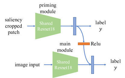
Figure 9: The architecture of our model for NICO experiments. We use a shared ResNet18 as the feature extractor. Use the output logits of priming module as $\zeta$ and feed it through a Relu layer to main module.

Training Details We use BASNet (Qin et al., 2019) as the key input extractor $k(\cdot)$, which is an unsupervised saliency detection model. We use Cross-Entropy loss and SGD optimizer to jointly train our model for 200 epochs. The initial learning rate is set to 0.05 and decays by 0.2 at 80, 120 and 160 epochs. We set the minibatch size to 128. We select the best hyper-parameters according to the validation accuracy and then test the models on the test set.

Appendix H Additional Details on CARLA Experiments

In Section 4, we briefly introduce the experiment setup of CARLA. More details are introduced below.

Data Collection. The CARLA100 dataset (Codevilla et al., 2019) is collected by a PID controller. During collecting, 10% expert actions are perturbed by noise (Laskey et al., 2017). We use three cameras: a forward-facing one and two lateral cameras facing 30 degrees away towards left or right (Bojarski et al., 2016). Both noise injection and multiple cameras are common data augmentation techniques to alleviate distributional shift in autonomous driving.

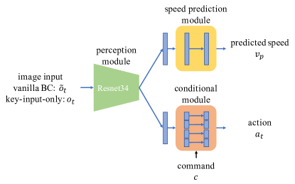
Figure 10: The conditional imitation learning architecture we used as our backbone. The input of vanilla BC is the observation history, denoted as $\tilde{o}_{t}$ for simplicity, and the input of key-input-only is the current observation $o_{t}$.

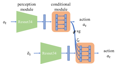
Figure 11: The architecture of our method. For simplicity, we omit the speed prediction module and the input command when drawing the figures, and sg means stop-gradient.

Architectures. We use the backbone in conditional imitation learning framework CILRS (Codevilla et al., 2019) as our backbone. The only difference is that our model does not have the input speed (to create a pure POMDP (Wen et al., 2021)). As shown in Figure 10, vanilla BC and key-input-only use the same architecture with different inputs, $\tilde{o}_{t}$ and $o_{t}$. Illustrated in Figure 11, our method integrates them together by concatenating the output of priming module with the features of the penultimate FC layer of main module. Moreover, the architectures of early fusion model and middle fusion model mentioned in Section4.4 are shown in Figure 12. In particular, early fusion means we concatenate the priming variable $\zeta$ with the input images, and middle fusion means that we concatenate it with the output feature of Resnet.

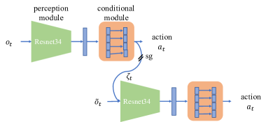
(a) early fusion

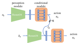
(b) middle fusion

Figure 12: The architectures of the early fusion model and middle fusion we study in Section 4.4.

Training Details. We use the $L_{1}$ loss to train all the models. We use Adam optimizer, set the initial learning rate to $2\times 10^{-4}$ and decay the learning rate by 0.1 whenever the loss value no longer decreases for 5000 gradient steps. We set the minibatch size to 160 and train all the models until convergence (the learning rate equal to $1\times 10^{-7}$). Furthermore, we apply several commonly used techniques to our training process. We utilize the noise injection (Laskey et al., 2017) and multi-camera data augmentation (Bojarski et al., 2016; Giusti et al., 2015) to alleviate the distribution shift in offline imitation learning. All the models use the speed regularization (Codevilla et al., 2019) to address the copycat problem (also called inertia problem in their paper) to some extent. And we use ImageNet pretrained ResNet34 (Deng et al., 2009; He et al., 2016) as the perception module to get a better initialization (Codevilla et al., 2019) and the weighted control loss to balance the models’ attention to each action dimension. Furthermore, different from the previous works (Codevilla et al., 2018, 2019; Wen et al., 2021), we use two-dimensional action space $a\in\left[-1,1\right]^{2}$ for steering and acceleration, where the positive acceleration value means applying throttle and the negative one means braking. We empirically find that using acceleration as output modality is better than predicting throttle and brake separately among all baselines (except FCA) and our method.

Appendix I Additional Details on Mujoco Experiments

Data Collection. We first train an RL expert with PPO (Schulman et al., 2017) and use it to generate expert demonstration by rolling out in the environment. Specifically, we collect 10k samples for Ant and Walker2D, and 20k for Hopper based on imitation difficulty.

Architectures. We follow a simple design for network architectures, shown in Figure 13. For both the priming module and main module, we use a three-layer MLP network. We concatenate the output action from the priming module to the output of main module, and input that to another fully-connected layer for the final output action.

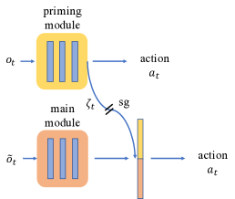
Figure 13: The architecture of our method for MuJoCo experiments, where sg means stop-gradient.

Training Details. We use MSE loss and Adam optimizer to train all models. We use a learning rate of 1e-4 for both HalfCheetah and Ant, and 1e-5 for Hopper and use linear learning rate decay. For each environment, we train it for 1000 epochs until convergence. We set the minibatch size to 64. We train each method three times, and report the mean and standard deviation of evaluation rewards for the last three evaluation steps.

Appendix J Theorem Version for Proposition 3.1

We next formally state our theorem, starting from the basic definitions and assumptions.

J.1 Theorem Statement

Data Distribution. Let $(\bm{x},y)\sim\mathcal{P}_{in}\subset\mathbb{R}^{d}\times\mathbb{R}$, $(\bm{z},y)\sim\mathcal{P}_{out}\subset\mathbb{R}^{d}\times\mathbb{R}$ denote the input and the corresponding label in the training region and test region, respectively. Without loss of generality, we assume that $\mathbb{E}\bm{x}=\mathbb{E}\bm{z}=\bm{0}$, and $|y|\leq O(1)$ is bounded almost surely. For simplicity, we assume the data covariance satisfies $\Sigma=\Sigma_{\bm{x}}=\Sigma_{\bm{z}}$, and assume that $\operatorname{Tr}(\Sigma)=d$, $\sigma_{min}(\Sigma)=O(1)$, and $\sigma_{max}(\Sigma)=O(1)$. We assume that the re-scaled input $\Sigma^{-1/2}\bm{x}$ and $\Sigma^{-1/2}\bm{z}$ has independent and $O(1)$-subGaussian coordinates.

Denote the optimal linear estimator as $\beta^{*}$, which satisfies $\mathbb{E}_{\mathcal{P}_{in}}(y-\bm{x}^{\top}\beta^{*})^{2}=\min_{\beta}\mathbb{E}_{\mathcal{P}_{in}}(y-\bm{x}^{\top}\beta)^{2}$, and $\|\beta^{*}\|=O(1)$. We assume that the residual $\bm{\epsilon}=y-\bm{x}^{\top}\beta^{*}$ is mean zero, independent, $O(1)$-subgaussian conditional on $\bm{x}$ with $\mathbb{E}\bm{\epsilon}^{2}|\bm{x}=O(1)$. Given the dataset with $n$ pairs independently sampled from $\mathcal{P}_{in}$ and $\mathcal{P}_{out}$, we denote the empirical distribution by $\hat{\mathcal{P}}_{1}^{n}$ and $\hat{\mathcal{P}}_{2}^{n}$. We assume that the sample size satisfies $n\gg d$ and $n=d^{O(1)}$, and the corresponding design matrix is diagonalizable.

Model. We consider a two-layer fully-connected neural network with $m$ hidden neurons: $f(\bm{x};\bm{w},v):=\frac{1}{\sqrt{m}}\sum_{r=1}^{m}v_{r}\sigma(\bm{w}_{r}^{\top}\bm{x}/\sqrt{d})$ with symmetric initialization, where the activation $\sigma$ is smooth or piece-wise linear. In this paper, Neural Tangent Kernels (NTK) are applied to approximate the neural networks, where $\{\bm{w}_{r}\}$ is trainable and $\{v_{r}\}$ is fixed following the regime in Arora et al. (2019). For the training process with constant step size (sufficiently small) and $\ell_{2}$ loss, we derive the following Theorem J.1 for the function $f_{NTK}(\cdot)$ trained at time $t$

For the neural networks, we consider a two-layer fully connect one and use the matrix formulation $(\bm{W},\bm{v})$ as follows:

$$f(\bm{x};\bm{W},\bm{v})=\frac{1}{\sqrt{m}}\sum_{r=1}^{m}v_{r}\sigma(\bm{w}_{r}^{\top}\bm{x}/\sqrt{d})=\frac{1}{\sqrt{m}}\bm{v}^{\top}\sigma(\bm{W}\bm{x}/\sqrt{d}).$$

Linear Kernels. Follong Hu et al. (2020b), when considering linear models, we consider the linear feature On the other hand, we consider the linear feature

$$\phi_{LIN}(X)=\frac{1}{\sqrt{d}}\left[\begin{array}[]{c}\zeta\bm{x}\\ \nu\end{array}\right],$$

where $\zeta=\mathbb{E}[\sigma^{\prime}(g)]$ and $\nu=\mathbb{E}[g\sigma^{\prime}(g)]\cdot\sqrt{\operatorname{Tr}[\Sigma^{2}]/d}$. We denote the function trained using linear kernels at time $t$ as $f_{LIN}^{(t)}$, and define the corresponding predictions on $\bm{X}$ and $\bm{Z}$ as $\hat{Y}_{LIN}(\bm{X})$ and $\hat{Y}_{LIN}(\bm{Z})$.

Neural Tangent Kernels. We consider a neural tangent kernel using the following feature

$$\phi_{NTK}(X)=\operatorname{Vec}\left(\frac{\partial f(\bm{x};\bm{W},\bm{v})}{\partial\bm{W}}\right).$$

We denote the function trained using neural tangent kernels at time $t$ as $f_{NTK}^{(t)}$, and define the corresponding predictions on $\bm{X}$ and $\bm{Z}$ as $\hat{Y}_{NTK}(\bm{X})$ and $\hat{Y}_{NTK}(\bm{Z})$.

Symmetric Initialization In this paper, we apply the symmetric initialization, $\bm{w}_{i}\sim\mathcal{N}(\bm{0},\bm{I}_{d})$ and $v_{i}\sim\operatorname{Unif}(\{1,-1\})$, $\bm{w}_{(i+m/2)}=\bm{w}_{i}$, $v_{(i+m/2)}=-v_{i}$, $i=1\dots,m/2$. This type of symmetric initializationfollowing (Chizat et al., 2019; Zhang et al., 2020; Hu et al., 2020a; Bai & Lee, 2020; Hu et al., 2020b) guarantees that $f(\bm{x};\bm{W},\bm{v})=0$ at initialization. Therefore, we can regard the corresponding NTK is trained by starting with initialization $\bm{0}$.

J.2 The Main Theorem

We now provide the main theorem in Theorem J.1

Theorem J.1.

Let $\alpha\in(0,1/4)$ be a fixed constant. Let $h(\bm{x})=\bm{x}^{\top}\beta^{*}:\mathbb{R}^{d}\to\mathbb{R}$ denote a linear model, and $s:\mathbb{R}^{d}\to\mathbb{R}$ denote another model. We assume the following (A1-A3) assumptions:

1. In the training region $\mathcal{P}_{in}$, function $f$ and $s$ are both close to the ground truth, $\|y-h(\bm{x})\|_{\mathcal{P}_{in}}\leq\epsilon$, and $\|y-s(\bm{x})\|_{\mathcal{P}_{in}}\leq\epsilon$.

2. In the test region $\mathcal{P}_{out}$, function $f$ and $s$ are separable, $\|s(\bm{z})-h(\bm{z})\|_{\mathcal{P}_{out}}\geq O(1)$.

3. The width of the neural network satisfies $m=\Omega(d^{1+\alpha})$

Then for the model $f_{NTK}^{t}(\cdot)$ trained by neural tangent kernel at time $t=\Theta(d^{1+\frac{1}{3}\alpha})$, satisfies the following statements (C1-C2) hold with high probability:

1. In training region $\mathcal{P}_{in}$, the trained model reaches small training error, $\|f_{NTK}(\bm{x})-y\|_{\hat{\mathcal{P}}_{1}^{n}}-\epsilon\lesssim d^{-\frac{1}{3}\alpha}+\sqrt{\frac{d}{n}}$.

2. In test region $\mathcal{P}_{out}$, the trained model is closer to $f$ instead of $s$, $\|f_{NTK}(\bm{z})-h\|_{\hat{\mathcal{P}}_{2}^{n}}\lesssim d^{-\frac{1}{3}\alpha}+\sqrt{\frac{d}{n}}$ and $\|f_{NTK}(\bm{z})-s\|_{\hat{\mathcal{P}}_{2}^{n}}=\Omega(1)$.

J.3 Proof

In this section, We provide the whole proof of Theorem J.1.

J.4 Proof

Proof.

We combine the following Three Lemmas to reach the final conclusion of Theorem J.1. We first show in Lemma J.2 that the model trained by NTK is indeed close to the model trained by linear predictions in the train region $\mathcal{P}_{in}$. We then show in Lemma J.3 that the trained model is also close to the model trained by linear predictions in the test region $\mathcal{P}_{out}$. We finally show in Lemma J.4 that linear models can approximate the ground truth function for a proper time $t$. ∎

Lemma J.2 (Bounding difference between NTK and linear predictions (train region)).

Under the settings in Theorem J.1, the prediction of the NTK models ($\hat{Y}_{NTK}(\bm{X})$) is close to the prediction of linear models ($\hat{Y}_{LIN}(\bm{X})$), namely,

$$\frac{1}{\sqrt{n}}\left\|\hat{Y}_{NTK}(\bm{X})-\hat{Y}_{LIN}(\bm{X})\right\|\lesssim d^{-\frac{1}{3}\alpha}.$$

Proof of Lemma J.2.

Note that NKT regimes is overparameterized while linear regime is underparameterized. We derive from Proposition J.5 that the prediction (on training set) from neural tangent kernel and the linear kernel is

$$\begin{split}&\hat{Y}_{NTK}(\bm{X})=\left[I-\left[I-\frac{\lambda}{n}\phi_{NTK}(X)\phi_{NTK}^{\top}(X)\right]^{t}\right]Y,\\ &\hat{Y}_{LIN}(\bm{X})=\left[I-\left[I-\frac{\lambda}{n}\phi_{LIN}(X)\phi_{LIN}^{\top}(X)\right]^{t}\right]Y.\end{split}$$

Note that function $(1-\lambda x)^{t}$ is $\lambda t$-Lipschitz, we have

$$\begin{split}&\frac{1}{\sqrt{n}}\left\|\hat{Y}_{NTK}(\bm{X})-\hat{Y}_{LIN}(\bm{X})\right\|\\ =&\frac{1}{\sqrt{n}}\left\|\left[\left[I-\frac{\lambda}{n}\phi_{LIN}(X)\phi_{LIN}^{\top}(X)\right]^{t}-\left[I-\frac{\lambda}{n}\phi_{NTK}(X)\phi_{NTK}^{\top}(X)\right]^{t}\right]Y\right\|,\\ \leq&\frac{1}{\sqrt{n}}\left\|\left[\left[I-\frac{\lambda}{n}\phi_{LIN}(X)\phi_{LIN}^{\top}(X)\right]^{t}-\left[I-\frac{\lambda}{n}\phi_{NTK}(X)\phi_{NTK}^{\top}(X)\right]^{t}\right]\right\|\left\|Y\right\|\\ \overset{(i)}{\leq}&\frac{1}{\sqrt{n}}\lambda t\frac{1}{n}\log(n)\left\|\phi_{LIN}(X)\phi_{LIN}^{\top}(X)-\phi_{NTK}(X)\phi_{NTK}^{\top}(X)\right\|\left\|Y\right\|\\ \overset{(ii)}{=}&\frac{1}{\sqrt{n}}\lambda t\frac{1}{n}\log(n)\cdot O\left(\frac{n}{d^{1+\alpha}}\right)\cdot O(\sqrt{n})\\ =&O\left(\lambda t\log(n)\frac{1}{d^{1+\alpha}}\right),\end{split}$$

where we apply Proposition J.7 in (i) and apply Proposition J.6 in (ii). And we use the fact that $y$ is bounded almost surely to get $\|Y\|\leq O(\sqrt{n})$. Due to the fact that $n=d^{O(1)}$ and $t=\Theta\left(d^{1+\frac{1}{3}\alpha}\right)$, we have

$$\begin{split}\frac{1}{\sqrt{n}}\left\|\hat{Y}_{NTK}(\bm{X})-\hat{Y}_{LIN}(\bm{X})\right\|\lesssim d^{-\frac{1}{3}\alpha}.\end{split}$$

∎

Lemma J.3 (Bounding difference between NTK and linear predictions (test region)).

Denote $\bm{Z}\in\mathbb{R}^{n\times p}$ the test samples independent sampled from distribution $\mathcal{P}_{out}$. Under the settings in Theorem J.1, the prediction of the NTK models ($\hat{Y}_{NTK}(\bm{Z})$) is close to the prediction of linear models ($\hat{Y}_{LIN}(\bm{Z})$) at test region with high probability, namely,

$$\frac{1}{\sqrt{n}}\left\|\hat{Y}_{NTK}(\bm{Z})-\hat{Y}_{LIN}(\bm{Z})\right\|\lesssim d^{-\frac{1}{3}\alpha}.$$

Proof of Lemma J.3..

Similar to the proof in Lemma J.2, the predictions are

$$\begin{split}&\hat{Y}_{NTK}(\bm{Z})\\ =&\phi_{NTK}(Z)\phi_{NTK}^{\top}(X)\left[I-\left[I-\frac{\lambda}{n}\phi_{NTK}(X)\phi_{NTK}^{\top}(X)\right]^{t}\right]\left[\phi_{NTK}(X)\phi_{NTK}^{\top}(X)\right]^{-1}Y,\\ &\hat{Y}_{LIN}(\bm{Z})\\ =&\phi_{LIN}(Z)\phi_{LIN}^{\top}(X)\left[I-\left[I-\frac{\lambda}{n}\phi_{LIN}(X)\phi_{LIN}^{\top}(X)\right]^{t}\right]\phi_{LIN}(X)\left[\phi_{LIN}(X)\phi_{LIN}^{\top}(X)\right]^{-2}\phi_{LIN}^{\top}(X)Y.\end{split}$$

We calculate that

$$\begin{split}&\hat{Y}_{NTK}(\bm{Z})-\hat{Y}_{LIN}(\bm{Z})\\ =&\phi_{NTK}(Z)\phi_{NTK}^{\top}(X)\left[I-\left[I-\frac{\lambda}{n}\phi_{NTK}(X)\phi_{NTK}^{\top}(X)\right]^{t}\right]\left[\phi_{NTK}(X)\phi_{NTK}^{\top}(X)\right]^{-1}Y\\ &-\phi_{LIN}(Z)\phi_{LIN}^{\top}(X)\left[I-\left[I-\frac{\lambda}{n}\phi_{LIN}(X)\phi_{LIN}^{\top}(X)\right]^{t}\right]\phi_{LIN}(X)\left[\phi_{LIN}(X)\phi_{LIN}^{\top}(X)\right]^{-2}\phi_{LIN}^{\top}(X)Y\\ =&\underline{\frac{\lambda}{n}\left[\phi_{NTK}(Z)\phi_{NTK}^{\top}(X)-\phi_{LIN}(Z)\phi_{LIN}^{\top}(X)\right]A_{1}Y}+\underline{\frac{\lambda}{n}\phi_{LIN}(Z)\phi_{LIN}^{\top}(X)[A_{1}-A_{2}]Y}\\ \triangleq&\text{①}+\text{②},\end{split}$$

where $A_{1}=\left[I-\left[I-\frac{\lambda}{n}\phi_{NTK}(X)\phi_{NTK}^{\top}(X)\right]^{t}\right]\left[\frac{\lambda}{n}\phi_{NTK}(X)\phi_{NTK}^{\top}(X)\right]^{-1}$, and
$A_{2}=\left[I-\left[I-\frac{\lambda}{n}\phi_{LIN}(X)\phi_{LIN}^{\top}(X)\right]^{t}\right]\phi_{LIN}(X)\left[\phi_{LIN}(X)\phi_{LIN}^{\top}(X)\right]^{-2}\phi_{LIN}^{\top}(X)$.

Bounding ①. We derive from Proposition J.8 that

$$\left\|\phi_{NTK}(Z)\phi_{NTK}^{\top}(X)-\phi_{LIN}(Z)\phi_{LIN}^{\top}(X)\right\|\lesssim\frac{n}{d^{1+\alpha}}.$$

We then calculate that the eigenvalues of the matrix $A_{1}$ can be bounded by

$$\frac{1-(1-\lambda\sigma_{i}^{t})}{\lambda\sigma_{i}}\leq t,$$

where $\sigma_{i}$ denotes the eigenvalues of matrix $\phi_{NTK}(Z)\phi_{NTK}^{\top}(X)$. Note that $\|\bm{Y}\|=O(\sqrt{n})$ due to the bounded assumption. Therefore, we have

$$\begin{split}&\text{①}\\ \leq&\frac{\lambda}{n}\left\|\phi_{NTK}(Z)\phi_{NTK}^{\top}(X)-\phi_{LIN}(Z)\phi_{LIN}^{\top}(X)\right\|\cdot\|A_{1}\|\cdot\|\bm{Y}\|\\ \lesssim&\frac{\lambda}{n}\cdot\frac{n}{d^{1+\alpha}}\cdot t\cdot\sqrt{n}\\ \lesssim&\left(\frac{t\sqrt{n}}{d^{1+\alpha}}\right).\end{split}$$ (1)

Bounding ②. We first use Proposition J.7 to bound $\|A_{1}-A_{2}\|$. The eigenvalues of $A_{1}$ and $A_{2}$ has the form of $(1-(1-\lambda\sigma_{i})^{t})/\lambda\sigma_{i}$ where $\sigma_{i}$ are the eigenvalues of $\phi_{NTK}(X)\phi_{NTK}^{\top}(X)$ and $phi_{LIN}(X)\phi_{LIN}^{\top}(X)$. From Proposition J.9, we see that the Lipschitz constant $L_{e}$ for function $e(x)=(1-(1-x)^{t})/x$ satisfies $L_{e}\lesssim t^{2}$. Therefore,

$$\begin{split}\|A_{1}-A_{2}\|&\lesssim t^{2}\log(n)\|\frac{\lambda}{n}\phi_{NTK}(X)\phi_{NTK}^{\top}(X)-\frac{\lambda}{n}\phi_{LIN}(X)\phi_{LIN}^{\top}(X)\|\\ &\lesssim t^{2}\cdot\frac{\lambda}{n}\cdot\frac{n}{d^{1+\alpha}}\\ &\lesssim t^{2}\frac{\lambda}{d^{1+\alpha}}\end{split}$$

Besides, we have that $\phi_{LIN}(Z)\phi_{LIN}^{\top}(X)\leq\|\phi_{LIN}(Z)\phi_{LIN}^{\top}(X)-\phi_{NTK}(Z)\phi_{NTK}^{\top}(X)\|+\|\phi_{NTK}(Z)\phi_{NTK}^{\top}(X)\|\lesssim n/d$, and therefore,

$$\begin{split}&\text{②}\\ =&\frac{\lambda}{n}\phi_{LIN}(Z)\phi_{LIN}^{\top}(X)[A_{1}-A_{2}]\bm{Y}\\ \leq&\frac{\lambda}{n}\|\phi_{LIN}(Z)\phi_{LIN}^{\top}(X)\|\cdot\|A_{1}-A_{2}\|\cdot\|\bm{Y}\|\\ \leq&\frac{\lambda}{n}\cdot O\left(\frac{n}{d}\right)\cdot O\left(t^{2}\frac{\lambda}{d^{1+\alpha}}\right)\cdot O(\sqrt{n})\\ \lesssim&\frac{t^{2}\sqrt{n}}{d^{2+\alpha}}.\end{split}$$ (2)

Therefore, we have that

$$\begin{split}\frac{1}{\sqrt{n}}\|\hat{Y}_{NTK}(\bm{Z})-\hat{Y}_{LIN}(\bm{Z})\|&\lesssim\frac{t}{d^{1+\alpha}}+\frac{t^{2}}{d^{2+\alpha}}\\ &\lesssim d^{-\frac{1}{3}\alpha}.\end{split}$$

where the last equation is due to $t=\Theta(d^{1+\frac{1}{3}\alpha})$. ∎

Lemma J.4 (Linear Training).

Denote $\hat{\bm{Y}}_{LIN}$ as the predictions of the linear predictors, $\bm{Y}(\bm{X})$ as the true label, and $\hat{\bm{Y}}^{*}_{LIN}$ as the best linear predictor. Under the settings in Theorem J.1, the predictions of $f_{LIN}$ is close to the ground truth in both $\mathcal{P}_{in}$ and $\mathcal{P}_{out}$. That is to say: with high probability

$$\begin{split}&\frac{1}{\sqrt{n}}\|\hat{Y}_{LIN}(\bm{X})-\bm{Y}(\bm{X})\|_{2}\lesssim\sqrt{\frac{d}{n}}+\epsilon,\\ &\frac{1}{\sqrt{n}}\|\hat{Y}_{LIN}(\bm{Z})-\hat{Y}_{LIN}^{*}(\bm{Z})\|_{2}\lesssim\sqrt{\frac{d}{n}}.\end{split}$$

Proof of Lemma J.4.

It suffices to bound the parameters trained by $\phi_{LIN}(\bm{X})$ with the optimal parameter $\bar{\beta}^{*}$. Note that ${\beta}_{LIN}^{*}$ is a re-scaled version of $\beta^{*}$, since $\phi_{LIN}(\bm{X})$ has a $1/\sqrt{d}$ scale. Therefore, informally, $\phi_{LIN}^{\top}(\bm{X})\phi_{LIN}(\bm{X})\approx\frac{1}{d}\bm{X}^{\top}\bm{X}$ and $\beta_{LIN}^{*}\approx\sqrt{d}\beta^{*}$.

We bound the difference of $\bm{Y}$ from the parameter perspective. Note that by gradient descent starting from initialization starting from initialization $\bm{0}$, by Proposition J.5, we have

$$\begin{split}&\beta_{LIN}^{(t)}=\left[I-\left[I-\frac{\lambda}{n}\phi_{LIN}^{\top}(\bm{X}_{1})\phi_{LIN}(\bm{X}_{1})\right]^{t}\right]\left[\phi_{LIN}^{\top}(\bm{X}_{1})\phi_{LIN}(\bm{X}_{1})\right]^{-1}\phi_{LIN}^{\top}(\bm{X}_{1})\bm{Y}.\end{split}$$

By plugging into $\bm{Y}=\bm{X}^{\top}\beta^{*}+\bm{\epsilon}=\phi_{LIN}(\bm{X})\beta_{LIN}^{*}+\bm{\epsilon}$ where $\bm{\epsilon}=\bm{Y}-\bm{X}^{\top}\beta$, it holds that

$$\begin{split}\beta_{LIN}^{(t)}=&[I-[I-\frac{\lambda}{n}\phi_{LIN}^{\top}(\bm{X}_{1})\phi_{LIN}(\bm{X}_{1})]^{t}]\beta_{LIN}^{*}\\ &+[I-[I-\frac{\lambda}{n}\phi_{LIN}^{\top}(\bm{X}_{1})\phi_{LIN}(\bm{X}_{1})]^{t}][\phi_{LIN}^{\top}(\bm{X}_{1})\phi_{LIN}(\bm{X}_{1})]^{-1}\phi_{LIN}^{\top}(\bm{X}_{1})\bm{\epsilon}.\end{split}$$

Therefore,

$$\begin{split}&\|\beta_{LIN}^{(t)}-\beta_{LIN}^{*}\|\\ \leq&\left\|\beta_{LIN}^{*}\right\|\left\|[I-\frac{\lambda}{n}\bm{X}_{1}^{\top}\bm{X}_{i}]^{t}\right\|\\ &+\left\|\left[I-\left[I-\frac{\lambda}{n}\phi_{LIN}^{\top}(\bm{X}_{1})\phi_{LIN}(\bm{X}_{1})\right]^{t}\right]\left[\phi_{LIN}^{\top}(\bm{X}_{1})\phi_{LIN}(\bm{X}_{1})\right]^{-1}\phi_{LIN}^{\top}(\bm{X}_{1})\bm{\epsilon}\right\|.\end{split}$$

Provided that $\log(1/\delta_{1})\leq n/c$, we know from Lemma J.10 that with probability at least $1-\delta_{1}$,

$$\frac{1}{d}\lesssim\frac{1}{n}\sigma_{min}\left(\phi_{LIN}^{\top}(\bm{X}_{1})\phi_{LIN}(\bm{X}_{1})\right)\leq\frac{1}{n}\sigma_{max}\left(\phi_{LIN}^{\top}(\bm{X}_{1})\phi_{LIN}(\bm{X}_{1})\right)\lesssim\frac{1}{d},$$

Therefore, given that $\lambda<1/\sigma_{n}(X^{\top}X)$ and $t\gg d$,

$$\begin{split}&\left\|[I-\frac{\lambda}{n}\phi_{LIN}^{\top}(\bm{X}_{1})\phi_{LIN}(\bm{X}_{1})]^{t}\right\|\leq c_{2}^{t/d}\lesssim O(1/\sqrt{n}),\end{split}$$

where $0<c_{2}<1$ is a given constant.

On the other hand, since $\epsilon_{i}$ is mean zero, independent, and $\sigma_{y}$-subGaussian with variance $\sigma^{2}$. Therefore, following Theorem 6.3.1 in Vershynin (2018), with probability at least $1-\delta_{2}$ (the probability is over $\bm{\epsilon}$ given $\bm{X}_{1}$),

$$\|H\bm{\epsilon}\|/\sigma\leq\|H\|_{F}+c_{3}\sigma_{\bm{x}}^{2}\|H\|\sqrt{\log(1/\delta_{3})},$$

where $H=\left[I-\left[I-\frac{\lambda}{n}\phi_{LIN}^{\top}(\bm{X}_{1})\phi_{LIN}(\bm{X}_{1})\right]^{t}\right]\left[\phi_{LIN}^{\top}(\bm{X}_{1})\phi_{LIN}(\bm{X}_{1})\right]^{-1}\phi_{LIN}^{\top}(\bm{X}_{1})$. Note that since $H\preceq\left[\phi_{LIN}^{\top}(\bm{X}_{1})\phi_{LIN}(\bm{X}_{1})\right]^{-1}\phi_{LIN}^{\top}(\bm{X}_{1})$, the eigenvalues of $H$ satisfies

$$\begin{split}\|H\|_{F}^{2}=\sum_{i=1}^{d}\sigma_{i}(H)^{2}\leq\sum_{i=1}^{d}\sigma_{i}(\left[\phi_{LIN}^{\top}(\bm{X}_{1})\phi_{LIN}(\bm{X}_{1})\right]^{-1}\phi_{LIN}^{\top}(\bm{X}_{1}))^{2}\leq\frac{d^{2}}{n},\\ \|H\|_{2}^{2}=\max_{i}\sigma_{i}(H)^{2}\leq\max_{i}\sigma_{i}(\left[\phi_{LIN}^{\top}(\bm{X}_{1})\phi_{LIN}(\bm{X}_{1})\right]^{-1}\phi_{LIN}^{\top}(\bm{X}_{1}))^{2}\leq\frac{d}{n}.\end{split}$$

Therefore, with probability at least $1-\delta_{2}$ with $\log(1/\delta_{3})\lesssim\sqrt{d}$,

$$\|H\bm{\epsilon}\|\lesssim\sqrt{d}\frac{\sqrt{d}+\sigma_{\bm{x}}^{2}\sqrt{\log(1/\delta_{3})}}{\sqrt{n}}\lesssim\frac{d}{\sqrt{n}}.$$

In summary, we have that with high probability

$$\|\beta_{LIN}^{(t)}-\beta_{LIN}^{*}\|\lesssim\|\beta_{LIN}^{*}\|^{2}c_{2}^{t/d}+\frac{d}{\sqrt{n}}\lesssim\frac{d}{\sqrt{n}}.$$

Therefore, due to the fact that $\|\bm{X}\|=O(\sqrt{n}/\sqrt{d})$ and $\|\bm{Z}\|=O(\sqrt{n}/\sqrt{d})$, we have that with high probability,

$$\begin{split}&\frac{1}{\sqrt{n}}\|\hat{\bm{Y}}_{LIN}(\bm{X})-\bm{Y}(\bm{X})\|_{2}\\ \leq&\frac{1}{\sqrt{n}}\|\hat{\bm{Y}}_{LIN}(\bm{X})-\hat{\bm{Y}}_{LIN}^{*}(\bm{X})\|_{2}+\|\hat{\bm{Y}}_{LIN}^{*}(\bm{X})-\bm{Y}(\bm{X})\|_{2}\\ \lesssim&\sqrt{\frac{d}{n}}+\epsilon,\\ &\frac{1}{\sqrt{n}}\|\hat{\bm{Y}}_{LIN}(\bm{Z})-\hat{\bm{Y}}_{LIN}^{*}(\bm{Z})\|_{2}\lesssim\sqrt{\frac{d}{n}}\\ .\end{split}$$

∎

Proposition J.5 (Trajectory Analysis).

For overparameterized linear regression ($n<p$) with gradient descent starting from $\theta^{(0)}=0$, we have

$$\theta^{(t)}=\bm{X}^{\top}\left[I-\left[I-\bm{X}\bm{X}^{\top}\right]^{t}\right]\left[\bm{X}\bm{X}^{\top}\right]^{-1}Y.$$

For underparameterized linear regression ($n>p$) with gradient descent starting from $\theta^{(0)}=0$, we have

$$\theta^{(t)}=\bm{X}^{\top}\left[I-\left[I-\bm{X}\bm{X}^{\top}\right]^{t}\right]\bm{X}\left[\bm{X}^{\top}\bm{X}\right]^{-2}\bm{X}^{\top}Y.$$

Proposition J.6 (Bounding the kernels, from Hu et al. (2020b), Proposition D.2).

Under the settings in Theorem J.1, the following inequality holds with high probability

$$\left\|\phi_{NTK}(X)\phi_{NTK}^{\top}(X)-\phi_{LIN}(X)\phi_{LIN}^{\top}(X)\right\|\lesssim\frac{n}{d^{1+\alpha}},$$

where the probability is taken over random initialization $\bm{W}(0)$ and the training data $\bm{X}$.

Proposition J.7 (Bounding difference from matrix function, from Theorem 11.4 in Aleksandrov & Peller (2011)).

For matrix function (function over eigenvalues) with Lipschitz constant $L$, we have that for any matrix $A,B\in\mathbb{R}^{n\times n}$, there exists a constant $C$ such that

$$\|f(A)-f(B)\|\leq CL\log(n)\|A-B\|.$$

Proposition J.8 (Bounding the cross kernels).

Under the settings in Theorem J.1, the following inequality holds with high probability

$$\left\|\phi_{NTK}(Z)\phi_{NTK}^{\top}(X)-\phi_{LIN}(Z)\phi_{LIN}^{\top}(X)\right\|\lesssim\frac{n}{d^{1+\alpha}},$$

where the probability is taken over random initialization $\bm{W}(0)$ and the training data $\bm{X}$.

Proof.

The proof is inspired by Hu et al. (2020b). We generalize the results of Theorem J.6 to the cross regimes. The proof is divided into three steps.

Step One. We firstly show that

$$\left\|\phi_{NTK}(Z)\phi_{NTK}^{\top}(X)-\mathbb{E}_{\bm{W}}\phi_{NTK}(Z)\phi_{NTK}^{\top}(X)\right\|\lesssim\frac{n}{d^{1+\alpha}},$$

This is due to Bernstein inequality. Due to the symmetric initialization, we first consider half number of the neurons which are guaranteed to be independent. For the $r$-th neuron, we denote

$$B^{(r)}=\left(\sigma^{\prime}\left(Zw_{r}/\sqrt{d}\right)\sigma^{\prime}\left(Xw_{r}/\sqrt{d}\right)\right)\odot\left(ZX^{\top}/\sqrt{d}\right).$$

Therefore, $\phi_{NTK}(Z)\phi_{NTK}^{\top}(X)=\frac{1}{m}\sum_{r=1}^{m}B^{(r)}$, and all neurons $\{B^{(r)}\},r=1,\dots,m/2$ are independent. Besides, we show that $B^{(r)}$ is bounded with high probability.

$$\begin{split}\left\|B^{(r)}\right\|&=\left\|\operatorname{diag}\left(\sigma^{\prime}\left(\bm{Z}w_{r}/\sqrt{d}\right)\right)\cdot\frac{\bm{Z}\bm{X}^{\top}}{d}\cdot\operatorname{diag}\left(\sigma^{\prime}\left(\bm{X}w_{r}/\sqrt{d}\right)\right)\right\|\\ &\leq\left\|\operatorname{diag}\left(\sigma^{\prime}\left(\bm{Z}w_{r}/\sqrt{d}\right)\right)\right\|\left\|\frac{\bm{X}}{\sqrt{d}}\right\|\left\|\frac{\bm{Z}}{\sqrt{d}}\right\|\left\|\operatorname{diag}\left(\sigma^{\prime}\left(\bm{X}w_{r}/\sqrt{d}\right)\right)\right\|\\ &\leq O(1)\cdot O\left(\sqrt{\frac{n}{d}}\right)\cdot O\left(\sqrt{\frac{n}{d}}\right)\cdot O(1)\\ &=O\left(\frac{n}{d}\right),\end{split}$$

where we use the fact that $\|\bm{Z}\|\lesssim n$ and $\|\bm{X}\|\lesssim n$ using the assumption that $X$ and $\bm{Z}$ are diagonalizable. Therefore, we derive that

$$\begin{split}&\left\|B^{(r)}\right\|\leq O(n/d)\\ &\left\|\mathbb{E}B^{(r)}\right\|\leq O(n/d)\\ &\left\|B^{(r)}-\mathbb{E}B^{(r)}\right\|\leq O(n/d)\\ &\left\|\sum_{r=1}^{m/2}\mathbb{E}[(B^{(r)}-\mathbb{E}B^{(r)})^{2}]\right\|\leq\sum_{r=1}^{m/2}\left\|\mathbb{E}(B^{(r)}-\mathbb{E}B^{(r)})^{2}\right\|\leq O(mn^{2}/d^{2})\end{split}$$

By Matrix Bernstein inequality, we have that

$$\mathbb{P}\left[\left\|\sum_{i=1}^{m/2}B^{(r)}-\mathbb{E}B^{(r)}\right\|\geq\frac{m}{2}\frac{n}{d^{1+\alpha}}\right]\ll 1,$$

where we use $m=\Omega(d^{1+\alpha})$ and $n=d^{O(1)}$.

Since $\phi_{NTK}(Z)\phi_{NTK}^{\top}(X)=\frac{1}{m}\sum_{r=1}^{m}B^{(r)}$ We rewrite the above inequality as follows: with high probability,

$$\begin{split}&\left\|\phi_{NTK}(Z)\phi_{NTK}^{\top}(X)-\mathbb{E}_{\bm{W}}\phi_{NTK}(Z)\phi_{NTK}^{\top}(X)\right\|\\ =&\left\|\frac{1}{m}\sum_{r=1}^{m}[B^{(r)}-\mathbb{E}B^{(r)}]\right\|\\ \leq&2\left\|\frac{1}{m/2}\sum_{r=1}^{m/2}[B^{(r)}-\mathbb{E}B^{(r)}]\right\|\\ \leq&\frac{1}{m}O(mn/d^{1+\alpha})\\ \lesssim&\frac{n}{d^{1+\alpha}}.\end{split}$$

Step Two. We secondly show that

$$\left\|\mathbb{E}_{\bm{W}}\phi_{NTK}(Z)\phi_{NTK}^{\top}(X)-\phi_{LIN}(Z)\phi_{LIN}^{\top}(X)\right\|\lesssim\frac{n}{d^{1+\alpha}}.$$

By defining $\Phi(a,b,c)=\mathbb{E}_{(u_{1},u_{2})\sim\mathcal{N}(0,\Lambda)}[\sigma^{\prime}(u_{1})\sigma^{\prime}(u_{2})]$, where $\Lambda=\left(\begin{array}[]{cc}a&c\\ c&b\end{array}\right)$, we rewrite that,

$$\begin{split}\left[\mathbb{E}_{\bm{W}}\phi_{NTK}(Z)\phi_{NTK}^{\top}(X)\right]_{ij}&=\frac{1}{d}z_{i}^{\top}x_{j}\cdot\mathbb{E}_{w\sim\mathcal{N}(0,I)}\left[\sigma^{\prime}(w^{\top}z_{i}/\sqrt{d})\sigma^{\prime}(w^{\top}x_{i}/\sqrt{d})^{\top}\right]\\ &=\frac{1}{d}z_{i}^{\top}x_{j}\Phi\left(\frac{\|z_{i}\|^{2}}{d},\frac{\|x_{i}\|^{2}}{d},\frac{z_{i}^{\top}x_{j}}{d}\right).\end{split}$$

Due to the assumptions on the data distribution and $n\gg d$, we have that $\frac{\|x_{i}\|^{2}}{d}=1\pm\tilde{O}(\frac{1}{\sqrt{d}})$, $\frac{\|z_{j}\|^{2}}{d}=1\pm\tilde{O}(\frac{1}{\sqrt{d}})$, and $\frac{z_{j}^{\top}x_{i}}{d}=\pm\tilde{O}(\frac{1}{\sqrt{d}})$. We apply Taylor expansion of $\Phi$ around (1, 1, 0), that is

$$\begin{split}&\Phi\left(\frac{\|z_{i}\|^{2}}{d},\frac{\|x_{i}\|^{2}}{d},\frac{z_{i}^{\top}x_{j}}{d}\right)\\ =&\Phi(1,1,0)+c_{1}\left(\frac{\|z_{i}\|^{2}}{d}-1\right)+c_{2}\left(\frac{\|x_{i}\|^{2}}{d}-1\right)+c_{3}\left(\frac{z_{i}^{\top}x_{j}}{d}\right)\pm\tilde{O}\left(\frac{1}{d}\right);\end{split}$$

Similar to the proof in Hu et al. (2020b), we have

$$\left\|\mathbb{E}_{\bm{W}}\phi_{NTK}(Z)\phi_{NTK}^{\top}(X)-\zeta^{2}\frac{ZX^{\top}}{d}-c_{3}\frac{Tr[\Sigma^{2}]}{d^{2}}\bm{1}\bm{1}^{\top}\right\|\leq\tilde{O}(\frac{n}{d^{1.25}}).$$

which is equivalent to

$$\left\|\mathbb{E}_{\bm{W}}\phi_{NTK}(Z)\phi_{NTK}^{\top}(X)-\phi_{LIN}(Z)\phi_{LIN}^{\top}(X)\right\|\lesssim\frac{n}{d^{1+\alpha}},$$

where $0<\alpha<1/4$.

Combining the two steps, we have that

$$\left\|\phi_{NTK}(Z)\phi_{NTK}^{\top}(X)-\phi_{LIN}(Z)\phi_{LIN}^{\top}(X)\right\|\lesssim\frac{n}{d^{1+\alpha}}.$$

∎

Proposition J.9.

Denote function $e(x)=\frac{1-(1-x)^{t}}{x}$, its Lipschitz constant satisfies $L_{e}\lesssim t^{2}$.

Proof of Proposition J.9.

Note that

$$\begin{split}e^{\prime}(x)&=\frac{tx(1-x)^{t-1}+(1-x)^{t}-1}{x^{2}}\\ &=\frac{t(1-x)^{t-1}}{x}+\frac{(1-x)^{t}-1}{x^{2}}\\ \end{split}$$

is decreasing with $x$, where $x\in(0,1)$ and $t\gg 3$. Therefore,

$$\begin{split}e^{\prime}(x)&\leq e^{\prime}(0)=-\frac{t(t-1)}{2}<0.\end{split}$$

Therefore, we consider $|e^{\prime}(x)|=-e^{\prime}(x)$. Note that by inequality $(1-x)^{t}\geq 1-tx$, we have

$$\begin{split}|e^{\prime}(x)|&=-e^{\prime}(x)\\ &=\frac{-tx(1-x)^{t-1}-(1-x)^{t}+1}{x^{2}}\\ &\leq\frac{-tx(1-({t-1})x)-(1-tx)+1}{x^{2}}\\ &=t(t-1)\\ &\lesssim t^{2}.\end{split}$$

Therefore, $L_{e}\lesssim t^{2}$.

∎

Proposition J.10.

Assume that $\Sigma_{\bm{x}}^{-1/2}\bm{x}_{i}$ is mean zero, independent, and $\sigma_{\bm{x}}$-subGaussian ($\|\cdot\|_{\psi_{2}}\leq\sigma_{\bm{x}}$), under the assumption $n\gg d$, then the maximal and minimal eigenvalue of $\bm{X}^{\top}\bm{X}$ satisfy: with probability at least $1-\delta$:

$$\|\Sigma_{\bm{x}}\|_{min}(n-C_{1}\sigma_{\bm{x}}^{2}\log(1/\delta))\lesssim\sigma_{n}(X^{\top}X)\leq\sigma_{1}(X^{\top}X)\lesssim\|\Sigma_{\bm{x}}\|_{max}(n+C_{1}\sigma_{\bm{x}}^{2}\log(1/\delta)),$$

where $\|\Sigma_{\bm{x}}\|_{min}$, $\|\Sigma_{\bm{x}}\|_{max}$ represent the minimal and maximal eigenvalues of $\Sigma_{\bm{x}}$ and $C_{1}$ is a universal constant independent of $n$ and $d$.

Proof.

Denote $A\triangleq\bm{X}\Sigma_{\bm{x}}^{-1/2}$ where $\bm{X}\in\mathbb{R}^{n\times d}$ is the corresponding design matrix. Note that each row of matrix $A$ is $A_{i}=\bm{x}_{i}^{\top}\Sigma_{\bm{x}}^{-1/2}$, which is independent and $\Sigma_{\bm{x}}$-subGaussian, and $\mathbb{E}A_{i}=\bm{0}$. Therefore, the maximum $\sigma_{1}(A)$ and minimal $\sigma_{n}(A)$ eigenvalue of $A$ satisfy the following inequality with probability at least $1-2\exp(-t^{2})$

$$\sqrt{n}-c_{1}\Sigma_{\bm{x}}(\sqrt{d}+t)\leq\sigma_{n}(A)\leq\sigma_{1}(A)\leq\sqrt{n}+c_{1}\Sigma_{\bm{x}}(\sqrt{d}+t),$$

where $c_{1}$ is a constant.

Due to the assumption $n\gg d$, it holds that with probability at least $1-\delta$,

$$\sqrt{n}-c_{1}\Sigma_{\bm{x}}\sqrt{\log(1/\delta)}\lesssim\sigma_{n}(A)\leq\sigma_{1}(A)\lesssim\sqrt{n}+c_{1}\Sigma_{\bm{x}}\sqrt{\log(1/\delta)}.$$

Since $\sigma_{i}(A^{\top}A)=\sigma_{i}(A)^{2}$, we have

$$n-c_{1}^{2}\Sigma_{\bm{x}}^{2}\log(1/\delta)\lesssim\sigma_{n}(A^{\top}A)\leq\sigma_{1}(A^{\top}A)\lesssim n+c_{1}^{2}\Sigma_{\bm{x}}^{2}\log(1/\delta).$$

Note that $A^{\top}A=\Sigma_{\bm{x}}^{-1/2}\bm{X}^{\top}\bm{X}\Sigma_{\bm{x}}^{-1/2}$, we have

$$\|\Sigma_{\bm{x}}\|_{min}(n-c_{1}^{2}\Sigma_{\bm{x}}^{2}\log(1/\delta))\lesssim\sigma_{n}(X^{\top}X)\leq\sigma_{1}(X^{\top}X)\lesssim\|\Sigma_{\bm{x}}\|_{max}(n+c_{1}^{2}\Sigma_{\bm{x}}^{2}\log(1/\delta)).$$

∎

References

- Ahuja et al. (2020) Ahuja, K., Shanmugam, K., Varshney, K., and Dhurandhar, A. Invariant risk minimization games. In Proceedings of the 37th International Conference on Machine Learning, Proceedings of Machine Learning Research, pp. 145–155. PMLR, 13–18 Jul 2020.
- Aleksandrov & Peller (2011) Aleksandrov, A. B. and Peller, V. V. Estimates of operator moduli of continuity. Journal of Functional Analysis, 261(10):2741–2796, 2011.
- Amodei et al. (2016) Amodei, D., Olah, C., Steinhardt, J., Christiano, P., Schulman, J., and Mané, D. Concrete problems in ai safety. arXiv preprint arXiv:1606.06565, 2016.
- Arjovsky et al. (2019) Arjovsky, M., Bottou, L., Gulrajani, I., and Lopez-Paz, D. Invariant risk minimization. arXiv preprint arXiv:1907.02893, 2019.
- Arora et al. (2019) Arora, S., Du, S. S., Hu, W., Li, Z., and Wang, R. Fine-grained analysis of optimization and generalization for overparameterized two-layer neural networks. In Chaudhuri, K. and Salakhutdinov, R. (eds.), Proceedings of the 36th International Conference on Machine Learning, ICML 2019, 9-15 June 2019, Long Beach, California, USA, volume 97 of Proceedings of Machine Learning Research, pp. 322–332. PMLR, 2019.
- Bahng et al. (2020) Bahng, H., Chun, S., Yun, S., Choo, J., and Oh, S. J. Learning de-biased representations with biased representations. In International Conference on Machine Learning, pp. 528–539. PMLR, 2020.
- Bai & Lee (2020) Bai, Y. and Lee, J. D. Beyond linearization: On quadratic and higher-order approximation of wide neural networks. In 8th International Conference on Learning Representations, ICLR 2020, Addis Ababa, Ethiopia, April 26-30, 2020. OpenReview.net, 2020.
- Bansal et al. (2019) Bansal, M., Krizhevsky, A., and Ogale, A. ChauffeurNet: Learning to Drive by Imitating the Best and Synthesizing the Worst. Robotics: Science & Systems (RSS), art. arXiv:1812.03079, 2019.
- Bargh & Chartrand (2014) Bargh, J. A. and Chartrand, T. L. The mind in the middle: A practical guide to priming and automaticity research. 2014.
- Bargh et al. (1996) Bargh, J. A., Chen, M., and Burrows, L. Automaticity of social behavior: Direct effects of trait construct and stereotype activation on action. Journal of personality and social psychology, 71(2):230, 1996.
- Beery et al. (2018) Beery, S., Van Horn, G., and Perona, P. Recognition in terra incognita. In Proceedings of the European Conference on Computer Vision (ECCV), pp. 456–473, 2018.
- Bickel et al. (2009) Bickel, S., Brückner, M., and Scheffer, T. Discriminative learning under covariate shift. J. Mach. Learn. Res., 10:2137–2155, 2009.
- Bojarski et al. (2016) Bojarski, M., Testa, D. D., Dworakowski, D., Firner, B., Flepp, B., Goyal, P., Jackel, L. D., Monfort, M., Muller, U., Zhang, J., Zhang, X., Zhao, J., and Zieba, K. End to end learning for self-driving cars. CoRR, abs/1604.07316, 2016.
- Brown et al. (2020) Brown, T. B., Mann, B., Ryder, N., Subbiah, M., Kaplan, J., Dhariwal, P., Neelakantan, A., Shyam, P., Sastry, G., Askell, A., et al. Language models are few-shot learners. arXiv preprint arXiv:2005.14165, 2020.
- Buolamwini & Gebru (2018) Buolamwini, J. and Gebru, T. Gender shades: Intersectional accuracy disparities in commercial gender classification. In Conference on fairness, accountability and transparency, pp. 77–91. PMLR, 2018.
- Cadene et al. (2019) Cadene, R., Dancette, C., Cord, M., Parikh, D., et al. Rubi: Reducing unimodal biases for visual question answering. Advances in neural information processing systems, 32:841–852, 2019.
- Cao et al. (2011) Cao, B., Ni, X., Sun, J.-T., Wang, G., and Yang, Q. Distance metric learning under covariate shift. In IJCAI, 2011.
- Chen et al. (2020) Chen, D., Zhou, B., Koltun, V., and Krähenbühl, P. Learning by cheating. In Conference on Robot Learning, pp. 66–75. PMLR, 2020.
- Chizat et al. (2019) Chizat, L., Oyallon, E., and Bach, F. R. On lazy training in differentiable programming. In Wallach, H. M., Larochelle, H., Beygelzimer, A., d’Alché-Buc, F., Fox, E. B., and Garnett, R. (eds.), Advances in Neural Information Processing Systems 32: Annual Conference on Neural Information Processing Systems 2019, NeurIPS 2019, December 8-14, 2019, Vancouver, BC, Canada, pp. 2933–2943, 2019.
- Clark et al. (2019) Clark, C., Yatskar, M., and Zettlemoyer, L. Don’t take the easy way out: Ensemble based methods for avoiding known dataset biases. In Proceedings of the 2019 Conference on Empirical Methods in Natural Language Processing and the 9th International Joint Conference on Natural Language Processing (EMNLP-IJCNLP), pp. 4069–4082. Association for Computational Linguistics, November 2019.
- Codevilla et al. (2018) Codevilla, F., Miiller, M., López, A., Koltun, V., and Dosovitskiy, A. End-to-end driving via conditional imitation learning. In 2018 IEEE International Conference on Robotics and Automation (ICRA), pp. 1–9. IEEE, 2018.
- Codevilla et al. (2019) Codevilla, F., Santana, E., López, A. M., and Gaidon, A. Exploring the limitations of behavior cloning for autonomous driving. In Proceedings of the IEEE International Conference on Computer Vision, pp. 9329–9338, 2019.
- de Haan et al. (2019) de Haan, P., Jayaraman, D., and Levine, S. Causal confusion in imitation learning. Advances in Neural Information Processing Systems, 32:11698–11709, 2019.
- Delage & Ye (2010) Delage, E. and Ye, Y. Distributionally robust optimization under moment uncertainty with application to data-driven problems. Oper. Res., 58:595–612, 2010.
- Deng et al. (2009) Deng, J., Dong, W., Socher, R., Li, L.-J., Li, K., and Fei-Fei, L. Imagenet: A large-scale hierarchical image database. In 2009 IEEE conference on computer vision and pattern recognition, pp. 248–255. Ieee, 2009.
- DeVries & Taylor (2017) DeVries, T. and Taylor, G. W. Improved regularization of convolutional neural networks with cutout. arXiv preprint arXiv:1708.04552, 2017.
- Dosovitskiy et al. (2017) Dosovitskiy, A., Ros, G., Codevilla, F., Lopez, A., and Koltun, V. CARLA: An open urban driving simulator. In Proceedings of the 1st Annual Conference on Robot Learning, pp. 1–16, 2017.
- Duchi & Namkoong (2021) Duchi, J. C. and Namkoong, H. Learning models with uniform performance via distributionally robust optimization. The Annals of Statistics, 49(3):1378–1406, 2021.
- Geirhos et al. (2018) Geirhos, R., Temme, C. R. M., Rauber, J., Schütt, H. H., Bethge, M., and Wichmann, F. A. Generalisation in humans and deep neural networks. In Bengio, S., Wallach, H., Larochelle, H., Grauman, K., Cesa-Bianchi, N., and Garnett, R. (eds.), Advances in Neural Information Processing Systems, volume 31. Curran Associates, Inc., 2018.
- Geirhos et al. (2019) Geirhos, R., Rubisch, P., Michaelis, C., Bethge, M., Wichmann, F. A., and Brendel, W. Imagenet-trained cnns are biased towards texture; increasing shape bias improves accuracy and robustness. In ICLR. OpenReview.net, 2019.
- Geirhos et al. (2020) Geirhos, R., Jacobsen, J.-H., Michaelis, C., Zemel, R., Brendel, W., Bethge, M., and Wichmann, F. A. Shortcut learning in deep neural networks. Nature Machine Intelligence, 2(11):665–673, 2020.
- Giusti et al. (2015) Giusti, A., Guzzi, J., Cireşan, D. C., He, F.-L., Rodríguez, J. P., Fontana, F., Faessler, M., Forster, C., Schmidhuber, J., Di Caro, G., et al. A machine learning approach to visual perception of forest trails for mobile robots. IEEE Robotics and Automation Letters, 1(2):661–667, 2015.
- He et al. (2019) He, H., Zha, S., and Wang, H. Unlearn dataset bias in natural language inference by fitting the residual. CoRR, abs/1908.10763, 2019.
- He et al. (2016) He, K., Zhang, X., Ren, S., and Sun, J. Deep residual learning for image recognition. In Proceedings of the IEEE conference on computer vision and pattern recognition, pp. 770–778, 2016.
- He et al. (2021) He, Y., Shen, Z., and Cui, P. Towards non-iid image classification: A dataset and baselines. Pattern Recognition, 110:107383, 2021.
- Hendrycks et al. (2020) Hendrycks, D., Basart, S., Mu, N., Kadavath, S., Wang, F., Dorundo, E., Desai, R., Zhu, T. L., Parajuli, S., Guo, M., Song, D. X., Steinhardt, J., and Gilmer, J. The many faces of robustness: A critical analysis of out-of-distribution generalization. ArXiv, abs/2006.16241, 2020.
- Hu et al. (2020a) Hu, W., Li, Z., and Yu, D. Simple and effective regularization methods for training on noisily labeled data with generalization guarantee. In 8th International Conference on Learning Representations, ICLR 2020, Addis Ababa, Ethiopia, April 26-30, 2020. OpenReview.net, 2020a.
- Hu et al. (2020b) Hu, W., Xiao, L., Adlam, B., and Pennington, J. The surprising simplicity of the early-time learning dynamics of neural networks. In Larochelle, H., Ranzato, M., Hadsell, R., Balcan, M., and Lin, H. (eds.), Advances in Neural Information Processing Systems 33: Annual Conference on Neural Information Processing Systems 2020, NeurIPS 2020, December 6-12, 2020, virtual, 2020b.
- Hu et al. (2020c) Hu, W., Xiao, L., Adlam, B., and Pennington, J. The surprising simplicity of the early-time learning dynamics of neural networks. In Larochelle, H., Ranzato, M., Hadsell, R., Balcan, M. F., and Lin, H. (eds.), Advances in Neural Information Processing Systems, volume 33, pp. 17116–17128. Curran Associates, Inc., 2020c.
- Jacot et al. (2018) Jacot, A., Gabriel, F., and Hongler, C. Neural tangent kernel: Convergence and generalization in neural networks. In Bengio, S., Wallach, H., Larochelle, H., Grauman, K., Cesa-Bianchi, N., and Garnett, R. (eds.), Advances in Neural Information Processing Systems, volume 31. Curran Associates, Inc., 2018.
- Krueger et al. (2021a) Krueger, D., Caballero, E., Jacobsen, J.-H., Zhang, A., Binas, J., Priol, R. L., and Courville, A. C. Out-of-distribution generalization via risk extrapolation (rex). In ICML, 2021a.
- Krueger et al. (2021b) Krueger, D., Caballero, E., Jacobsen, J.-H., Zhang, A., Binas, J., Zhang, D., Le Priol, R., and Courville, A. Out-of-distribution generalization via risk extrapolation (rex). In International Conference on Machine Learning, pp. 5815–5826. PMLR, 2021b.
- Laskey et al. (2017) Laskey, M., Dragan, A., Lee, J., Goldberg, K., and Fox, R. Dart: Optimizing noise injection in imitation learning. In Conference on Robot Learning (CoRL), volume 2, pp. 12, 2017.
- McCoy et al. (2019) McCoy, T., Pavlick, E., and Linzen, T. Right for the wrong reasons: Diagnosing syntactic heuristics in natural language inference. In Proceedings of the 57th Annual Meeting of the Association for Computational Linguistics, pp. 3428–3448. Association for Computational Linguistics, July 2019.
- Muhammad & Yeasin (2020) Muhammad, M. B. and Yeasin, M. Eigen-cam: Class activation map using principal components. In 2020 International Joint Conference on Neural Networks (IJCNN), pp. 1–7. IEEE, 2020.
- Muller et al. (2006) Muller, U., Ben, J., Cosatto, E., Flepp, B., and Cun, Y. L. Off-road obstacle avoidance through end-to-end learning. In Advances in neural information processing systems, pp. 739–746. Citeseer, 2006.
- Niven & Kao (2019) Niven, T. and Kao, H.-Y. Probing neural network comprehension of natural language arguments. In Proceedings of the 57th Conference of the Association for Computational Linguistics, pp. 4658–4664. Association for Computational Linguistics, July 2019.
- Oliva & Torralba (2007) Oliva, A. and Torralba, A. The role of context in object recognition. Trends in cognitive sciences, 11(12):520–527, 2007.
- Ortega et al. (2021) Ortega, P. A., Kunesch, M., Delétang, G., Genewein, T., Grau-Moya, J., Veness, J., Buchli, J., Degrave, J., Piot, B., Perolat, J., et al. Shaking the foundations: delusions in sequence models for interaction and control. arXiv preprint arXiv:2110.10819, 2021.
- Pearl (1995) Pearl, J. Causal diagrams for empirical research. Biometrika, 82(4):669–688, 1995.
- Prakash et al. (2021) Prakash, A., Chitta, K., and Geiger, A. Multi-modal fusion transformer for end-to-end autonomous driving. In Proceedings of the IEEE/CVF Conference on Computer Vision and Pattern Recognition (CVPR), pp. 7077–7087, June 2021.
- Qin et al. (2019) Qin, X., Zhang, Z., Huang, C., Gao, C., Dehghan, M., and Jagersand, M. Basnet: Boundary-aware salient object detection. In The IEEE Conference on Computer Vision and Pattern Recognition (CVPR), June 2019.
- Rosenfeld et al. (2018) Rosenfeld, A., Zemel, R., and Tsotsos, J. K. The elephant in the room. arXiv preprint arXiv:1808.03305, 2018.
- Ross et al. (2011) Ross, S., Gordon, G. J., and Bagnell, J. A. A reduction of imitation learning and structured prediction to no-regret online learning. Journal of Machine Learning Research, 15:627–635, 2011. ISSN 15324435.
- Rubin (1974) Rubin, D. B. Estimating causal effects of treatments in randomized and nonrandomized studies. Journal of educational Psychology, 66(5):688, 1974.
- Rubin (1978) Rubin, D. B. Bayesian inference for causal effects: The role of randomization. The Annals of statistics, pp. 34–58, 1978.
- Sagawa et al. (2019) Sagawa, S., Koh, P. W., Hashimoto, T. B., and Liang, P. Distributionally robust neural networks for group shifts: On the importance of regularization for worst-case generalization. ArXiv, abs/1911.08731, 2019.
- Schölkopf et al. (2012) Schölkopf, B., Janzing, D., Peters, J., Sgouritsa, E., Zhang, K., and Mooij, J. On causal and anticausal learning. arXiv preprint arXiv:1206.6471, 2012.
- Schrittwieser et al. (2020) Schrittwieser, J., Antonoglou, I., Hubert, T., Simonyan, K., Sifre, L., Schmitt, S., Guez, A., Lockhart, E., Hassabis, D., Graepel, T., et al. Mastering atari, go, chess and shogi by planning with a learned model. Nature, 588(7839):604–609, 2020.
- Schulman et al. (2017) Schulman, J., Wolski, F., Dhariwal, P., Radford, A., and Klimov, O. Proximal policy optimization algorithms. arXiv preprint arXiv:1707.06347, 2017.
- Shah et al. (2020) Shah, H., Tamuly, K., Raghunathan, A., Jain, P., and Netrapalli, P. The pitfalls of simplicity bias in neural networks. In Advances in Neural Information Processing Systems, volume 33, pp. 9573–9585. Curran Associates, Inc., 2020.
- Shen et al. (2021) Shen, Z., Liu, J., He, Y., Zhang, X., Xu, R., Yu, H., and Cui, P. Towards out-of-distribution generalization: A survey. ArXiv, abs/2108.13624, 2021.
- Spencer et al. (2021) Spencer, J., Choudhury, S., Venkatraman, A., Ziebart, B., and Bagnell, J. A. Feedback in imitation learning: The three regimes of covariate shift. arXiv preprint arXiv:2102.02872, 2021.
- Srivastava et al. (2014) Srivastava, N., Hinton, G., Krizhevsky, A., Sutskever, I., and Salakhutdinov, R. Dropout: a simple way to prevent neural networks from overfitting. The journal of machine learning research, 15(1):1929–1958, 2014.
- Todorov et al. (2012) Todorov, E., Erez, T., and Tassa, Y. Mujoco: A physics engine for model-based control. In 2012 IEEE/RSJ International Conference on Intelligent Robots and Systems, pp. 5026–5033. IEEE, 2012.
- Vershynin (2018) Vershynin, R. High-Dimensional Probability: An Introduction with Applications in Data Science. Cambridge Series in Statistical and Probabilistic Mathematics. Cambridge University Press, 2018. doi: 10.1017/9781108231596.
- Wang et al. (2021a) Wang, J., Lan, C., Liu, C., Ouyang, Y., and Qin, T. Generalizing to unseen domains: A survey on domain generalization. In IJCAI, 2021a.
- Wang et al. (2021b) Wang, T., Zhou, C., Sun, Q., and Zhang, H. Causal attention for unbiased visual recognition. In Proceedings of the IEEE/CVF International Conference on Computer Vision (ICCV), 2021b.
- Weingarten et al. (2016) Weingarten, E., Chen, Q., McAdams, M., Yi, J., Hepler, J., and Albarracín, D. From primed concepts to action: A meta-analysis of the behavioral effects of incidentally presented words. Psychological bulletin, 142(5):472, 2016.
- Wen et al. (2020) Wen, C., Lin, J., Darrell, T., Jayaraman, D., and Gao, Y. Fighting copycat agents in behavioral cloning from observation histories. In Advances in Neural Information Processing Systems, volume 33, 2020.
- Wen et al. (2021) Wen, C., Lin, J., Qian, J., Gao, Y., and Jayaraman, D. Keyframe-focused visual imitation learning. In Proceedings of the 38th International Conference on Machine Learning, Proceedings of Machine Learning Research. PMLR, 18–24 Jul 2021.
- Xu et al. (2021) Xu, Q., Zhang, R., Zhang, Y., Wang, Y., and Tian, Q. A fourier-based framework for domain generalization. In Proceedings of the IEEE/CVF Conference on Computer Vision and Pattern Recognition, pp. 14383–14392, 2021.
- Xu et al. (2019) Xu, Z.-Q. J., Zhang, Y., Luo, T., Xiao, Y., and Ma, Z. Frequency principle: Fourier analysis sheds light on deep neural networks. arXiv preprint arXiv:1901.06523, 2019.
- Zhang et al. (2021a) Zhang, A., McAllister, R. T., Calandra, R., Gal, Y., and Levine, S. Learning invariant representations for reinforcement learning without reconstruction. In International Conference on Learning Representations, 2021a.
- Zhang et al. (2017) Zhang, H., Cisse, M., Dauphin, Y. N., and Lopez-Paz, D. mixup: Beyond empirical risk minimization. arXiv preprint arXiv:1710.09412, 2017.
- Zhang et al. (2021b) Zhang, X., Cui, P., Xu, R., Zhou, L., He, Y., and Shen, Z. Deep stable learning for out-of-distribution generalization. In Proceedings of the IEEE/CVF Conference on Computer Vision and Pattern Recognition, pp. 5372–5382, 2021b.
- Zhang et al. (2020) Zhang, Y., Xu, Z. J., Luo, T., and Ma, Z. A type of generalization error induced by initialization in deep neural networks. In Lu, J. and Ward, R. (eds.), Proceedings of Mathematical and Scientific Machine Learning, MSML 2020, 20-24 July 2020, Princeton, NJ, USA, volume 107 of Proceedings of Machine Learning Research, pp. 144–164. PMLR, 2020.