CERN-TH-2022-099, DESY 22-102, ULB-TH/22-09

Minimal sterile neutrino dark matter

Abstract

We propose a novel mechanism to generate sterile neutrinos $\nu_{s}$ in the early Universe, by converting ordinary neutrinos $\nu_{\alpha}$ in scattering processes $\nu_{s}\nu_{\alpha}\to\nu_{s}\nu_{s}$. After initial production by oscillations, this leads to an exponential growth in the $\nu_{s}$ abundance. We show that such a production regime naturally occurs for self-interacting $\nu_{s}$, and that this opens up significant new parameter space where $\nu_{s}$ make up all of the observed dark matter. Our results provide strong motivation to further push the sensitivity of X-ray line searches, and to improve on constraints from structure formation.

Introduction.—

The existence of sterile neutrinos, putative particles that are uncharged under the standard model (SM) gauge interactions, is extremely well motivated. For example, such sterile states provide natural candidates [1, 2, 3, 4, 5] to explain the observed tiny nonzero neutrino masses [6]. If one of the sterile neutrinos has a mass in the keV range and is stable on cosmological time scales, furthermore, it is an excellent candidate for the dark matter (DM) in our Universe [7]. A smoking-gun signal for this scenario would be an astrophysical X-ray line, resulting from DM decaying into an active neutrino and a photon [8]. Such X-ray signatures are very actively being searched for, leading to ever more stringent limits on how much sterile and active neutrinos can mix [9] (while Refs. [10, 11] report a potential detection).

Sterile neutrinos can be produced by neutrino oscillations in the early Universe, which is known as the Dodelson-Widrow (DW) mechanism [12]. However, the region of parameter space where this mechanism produces an abundance of sterile neutrinos consistent with the entirety of the observed DM is excluded [13]. Alternative scenarios that remain viable include resonant production in the presence of a large lepton asymmetry [14], production by the decay of a scalar [15, 16, 17, 18, 19, 20], via an extended gauge sector [21, 22, 23], and production by oscillations modified by new self-interactions of the SM neutrinos [24, 25, 26, 27] or by interactions between the sterile neutrinos and a significantly heavier scalar in combination with a large lepton asymmetry [28].

All known viable mechanisms thus require new particles in addition to the sterile neutrino, either explicitly or implicitly (e.g., to ensure gauge invariance or to create a lepton asymmetry much larger than the observed baryon asymmetry). Our objective here is to propose a novel scenario that is minimal in the sense that it requires only a single real degree of freedom on top of the DM candidate.

Recently, some of us introduced a new generic DM production mechanism [29] that is characterized by DM particles transforming heat bath particles into more DM, thereby triggering an era of exponential growth of the DM abundance (see also Ref. [30]). As discussed there, one possibility to provide the necessary DM seed population for such a DM density evolution is through an initial freeze-in [31] period. In the scenario proposed in this article, instead, sterile neutrinos $\nu_{s}$ are initially generated through oscillations like in the DW mechanism and subsequently transform active neutrinos $\nu_{\alpha}$ through the process $\nu_{s}\nu_{\alpha}\to\nu_{s}\nu_{s}$. We demonstrate that such a scenario generically emerges when sterile neutrinos feel the presence of a dark force, and that this opens up significant portions of parameter space for sterile neutrino DM that may be detectable with upcoming experiments.

Model setup.—

A necessary requirement to realize DM production via exponential growth is $\langle\sigma v\rangle_{\rm tr}\gg\langle\sigma v\rangle_{\rm fi}$ [29], where $\langle\sigma v\rangle_{\rm tr}$ is the thermally averaged interaction rate for the transmission process, i.e. the conversion of a heat bath particle to a DM particle, and $\langle\sigma v\rangle_{\rm fi}$ is the corresponding quantity for the more traditional freeze-in process [31], where a pair of DM particles is produced from the collision of heat bath particles. Here we point out that a simple and generic way to realize this condition is a secluded dark sector [32, 33, 34, 35] where DM particles interact among each other via some mediator $\phi$, while interacting with the visible sector only through mixing by an angle $\theta$. In that case, both processes dominantly proceed via the $s$-channel exchange of $\phi$, resulting in $\langle\sigma v\rangle_{\rm tr}\propto\sin^{2}\theta$ and $\langle\sigma v\rangle_{\rm fi}\propto\sin^{4}\theta$. We note that such ‘secret interactions’ of sterile neutrinos have been studied in different cosmological contexts before [36, 37, 38, 39, 40, 41, 42, 43, 44, 45, 46, 47, 48, 49, 50, 51, 52, 53, 54, 55, 56, 57, 58, 59, 60, 61].

Motivated by these general considerations, we concentrate in the following on a single sterile neutrino $\nu_{s}$ interacting with a light scalar $\phi$, both singlets under the SM gauge group. Assuming Majorana masses for $\nu_{s}$ and the active neutrinos, $\nu_{\alpha}$, the relevant Lagrangian terms are given by

$$\mathcal{L}\supset-\frac{1}{2}\overline{\nu_{s}^{c}}m_{s}\nu_{s}-\overline{\nu_{\alpha}}m_{\alpha s}\nu_{s}-\frac{1}{2}\overline{\nu_{\alpha}}m_{\alpha}\nu_{\alpha}^{c}+\frac{y}{2}\overline{\nu_{s}^{c}}\phi\nu_{s}+\text{h.c.},$$ (1)

where repeated indices $\alpha$ are summed over and $\nu_{\alpha}$ ($\nu_{s}$) are left- (right-) handed spinors. We will concentrate on the case of heavy mediators, $m_{\phi}>2\,m_{s}$, for most of this article, but later also briefly discuss phenomenological consequences of lighter mediators. We checked that even for large mediator self-couplings, number-changing interactions like $2\phi\leftrightarrow 4\phi$ or $3\phi\leftrightarrow 4\phi$ do not qualitatively change our results and therefore neglect the scalar potential in all practical calculations. We further assume, for simplicity and concreteness, that $\nu_{s}$ dominantly mixes only with the active neutrino species $\nu_{e}$, and that $m_{s}\gg m_{\alpha}$. Expressed in terms of mass eigenstates, which for ease of notation we denote by the same symbols as flavor eigenstates, the interactions of the mediator then take the form

$$\mathcal{L}_{\phi}^{\text{I}}=\frac{y}{2}\phi\,\big{(}\cos^{2}\!\theta\,\overline{\nu_{s}^{c}}\nu_{s}-\sin(2\theta)\,\overline{\nu_{\alpha}}\nu_{s}+\sin^{2}\!\theta\,\overline{\nu_{\alpha}}\nu_{\alpha}^{c}\big{)}+\text{h.c.}$$ (2)

with $\theta\simeq m_{\alpha s}/m_{s}\ll 1$. The unsuppressed couplings among $\phi$ and $\nu_{s}$ turn out to be sufficiently strong to equilibrate the dark sector during the new exponential production phase that we consider below. On the other hand, mass-mixing-induced interactions between $\nu_{s}$ and electroweak gauge bosons are suppressed by the Fermi constant, $G_{F}$, and will only be relevant in setting the initial sterile neutrino abundance.

Figure 1: Relevant diagrams for (a) dark sector thermalization, $\nu_{s}\nu_{s}\!\to\!\phi^{*}\!\!\to\!\nu_{s}\nu_{s}$, (b) additionally increasing the dark sector number density between DW production and exponential growth, $\nu_{s}\nu_{s}\to\phi\phi$, and (c) exponential growth of DM, $\nu_{s}\nu_{\alpha}\!\to\!\phi^{*}\!\!\to\!\nu_{s}\nu_{s}$. Since $\phi$ is (almost) on-shell for (a) and (c), it is sufficient to include only the rates for $\nu_{s}\nu_{s}\leftrightarrow\phi$ and $\nu_{s}\nu_{\alpha}\to\phi$. See text for further details.

Evolution of $\nu_{s}$ number density.—

For an initially vanishing abundance, in particular, the interactions in Eq. (2) only allow freeze-in production of $\nu_{s}$. While the corresponding rate scales as $\sin^{4}\theta$, active-sterile neutrino oscillations at temperatures above and around $\Lambda_{\rm QCD}\sim 150$ MeV, in combination with neutral and charged current interactions with the SM plasma, lead to a production rate scaling as $\sin^{2}\theta$ [12]. Adopting results from Ref. [62], we use the $\nu_{s}$ number density, $n_{s}$, and energy density, $\rho_{s}\sim\langle p\rangle n_{s}$, that result from this DW production. Once it is completed, and in the absence of dark sector interactions, the expansion of the Universe will decrease these quantities as $n_{s}\propto a^{-3}$ and $\rho_{s}\propto a^{-4}$, respectively, where $a$ is the scale factor.

Some time later, various decay and scattering processes (cf. Fig. 1) become relevant due to the new interactions appearing in Eq. (2) and, for the parameter space we are interested in here, eventually thermalize the dark sector via the (inverse) decays $\nu_{s}\nu_{s}\leftrightarrow\phi$. From that point on, the phase-space densities of $\nu_{s}$ and $\phi$ follow Fermi-Dirac and Bose-Einstein distributions, respectively, that are described by a common dark sector temperature $T_{\mathrm{d}}$ as well as chemical potentials $\mu_{s}$ and $\mu_{\phi}$. Similar to the situation of freeze-out in a dark sector [63], the evolution of these quantities is determined by a set of Boltzmann equations for the number densities $n_{s,\phi}$ and total dark sector energy density $\rho=\rho_{\phi}+\rho_{s}$:

$$\dot{n}_{s}+3Hn_{s} =C_{n_{s}}\,,$$ (3)

$$\dot{n}_{\phi}+3Hn_{\phi} =C_{n_{\phi}}\,,$$ (4)

$$\dot{\rho}+3H(\rho+P) =C_{\rho}\,,$$ (5)

where $H\equiv\dot{a}/a$ is the Hubble rate, $P=P_{s}+P_{\phi}$ is the total dark sector pressure, and $C_{i}$ are the various collision operators (see Appendix for details). With $\phi\leftrightarrow\nu_{s}\nu_{s}$ in equilibrium, the chemical potentials are related by $2\mu_{s}=\mu_{\phi}$, allowing us to replace the first two of the above equations with a single differential equation for $\tilde{n}\equiv n_{s}+2n_{\phi}$. Noting that $\rho\propto a^{-4}$ and $\tilde{n}\propto a^{-3}$, both right before and after $\phi\leftrightarrow\nu_{s}\nu_{s}$ starts to dominate over the Hubble rate, the initial conditions to the coupled differential equations for $\tilde{n}$ and $\rho$ can then be determined at the end of DW production.

	$m_{s}$	$m_{\phi}$	$\sin^{2}(2\theta)$	$y$
BP1	12 keV	36 keV	$2.5\times 10^{-13}$	$1.905\times 10^{-4}$
BP2	20 keV	60 keV	$3.0\times 10^{-15}$	$1.602\times 10^{-3}$

Table 1: Parameter values for the two benchmark points considered in Fig. 2.

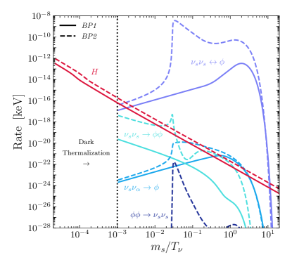
Figure 2: Cosmological evolution for the benchmark points BP1 (solid lines) and BP2 (dashed lines) specified in Tab. 1, as function of the inverse active neutrino temperature. Left: Comparison of Hubble rate $H$ (red) with the contribution of the indicated processes to $\left|C_{n_{s}}\right|/n_{s}$ (blue lines), see Appendix for details. Right: Corresponding evolution of $\nu_{s}$ (green) and $\phi$ (orange) abundances, and temperature ratio (dark gray, bottom panel). The dash-dotted gray line indicates the observed DM abundance [64].

In order to illustrate the subsequent evolution of the system, let us consider two concrete benchmark points, cf. Tab. 1, for which the sterile neutrinos obtain a relic density that matches the observed DM abundance of $\Omega_{\rm DM}h^{2}\simeq 0.12$ [64], with a mixing angle too small to achieve this with standard DW production. As demonstrated in Fig. 2, with solid (dashed) lines for BP1 (BP2), this leads to qualitatively different behaviors:

• Here the only additional process (beyond $\phi\leftrightarrow\nu_{s}\nu_{s}$) where the rate becomes comparable to $H$, at $m_{s}/T_{\nu}\sim 0.2$ with $T_{\nu}$ the active neutrino temperature, is $\nu_{s}\nu_{\alpha}\to\phi$ (left panel, light blue). This triggers exponential growth in the abundance for both $\nu_{s}$ and $\phi$ (right panel, green and orange) through $\nu_{s}\nu_{\alpha}\to\phi^{*}\to\nu_{s}\nu_{s}$, with $\phi$ being (almost) on shell, cf. Fig. 1 (c). Once $T_{\nu}\ll m_{\phi}$ the transmission process becomes inefficient and the final $\nu_{s}$ abundance is obtained. Afterwards, since both $\phi$ and $\nu_{s}$ are non-relativistic, the dark sector temperature decreases with $T_{\mathrm{d}}\propto a^{-2}$ both before and after kinetic decoupling (right panel, dark gray).

• In this case the larger coupling $y$ (needed to compensate for the smaller $\theta$) leads to another process impacting the evolution of the system: at $m_{s}/T_{\nu}\sim 0.01$, the rate for $\nu_{s}\nu_{s}\to\phi\phi$ (left panel, cyan, and Fig. 1 (b) starts to be comparable to $H$. As $\phi$ predominantly decays into $\nu_{s}\nu_{s}$ (left panel, orchid), this effectively transforms kinetic energy to rest mass by turning $2\nu_{s}$ to $4\nu_{s}$ – very similar to the reproductive freeze-in mechanism described by Refs. [28, 65, 66]. As expected, this leads to a significant drop in the temperature $T_{\mathrm{d}}$ (right panel, black). This process becomes inefficient for $T_{\mathrm{d}}\ll m_{\phi}$, due to the Boltzmann suppression of $\phi$. Subsequently, the rate for $\nu_{s}\nu_{\alpha}\to\phi$ (left panel, light blue) becomes comparable to $H$, leading to a phase of exponential growth in the same way as for BP1.

Observational constraints.—

Due to the mixing with active neutrinos, $\nu_{s}$ is not completely stable and subject to the same decays as in the standard scenario for keV-mass sterile neutrino DM. The strongest constraints on these decays come from a variety of X-ray line searches. We take the compilation of limits from Ref. [9], but only consider the overall envelope of constraints from Refs. [67, 68, 69, 70, 71, 72]. Furthermore, we consider projections for eROSITA [73], Athena [74], and eXTP [75].

Observations of the Lyman-$\alpha$ forest using light from distant quasars place stringent limits on a potential cutoff in the matter-power spectrum at small scales, where the scale of this cutoff is related to the time of kinetic decoupling, $t_{\mathrm{kd}}$. In our scenario, this is determined by DM self-interactions and we estimate $t_{\mathrm{kd}}$ from $Hn_{s}=C_{\nu_{s}\nu_{s}\to\nu_{s}\nu_{s}}$ [76], where the collision term $C_{\nu_{s}\nu_{s}\to\nu_{s}\nu_{s}}$ is stated in the Appendix. A full evaluation of Lyman-$\alpha$ limits would require evolving cosmological perturbations into the non-linear regime, which is beyond the scope of this work. Instead, we recast existing limits on the two main mechanisms that generate such a cutoff. At times $t<t_{\mathrm{kd}}$, DM self-scatterings prevent overdensities from growing on scales below the sound horizon $r_{\mathrm{s}}=\int_{0}^{t_{\mathrm{kd}}}\mathrm{d}t\,c_{\mathrm{s}}/a$, where $c_{\mathrm{s}}=\sqrt{\mathrm{d}P/\mathrm{d}\rho}$ is the speed of sound in the dark sector [77]. We use the results from Ref. [78] for cold DM in kinetic equilibrium with dark radiation (with $c_{\mathrm{s}}=1/\sqrt{3}$) to recast the current Lyman-$\alpha$ constraint on the mass of a warm DM (WDM) thermal relic $m_{\rm WDM}>1.9\,\mathrm{keV}$ [79] to the bound $r_{\mathrm{s}}<0.34\,\mathrm{Mpc}$. Overdensities are also washed out by the free streaming of DM after decoupling. We evaluate the free-streaming length as $\lambda_{\mathrm{fs}}=\int_{t_{\mathrm{kd}}}^{t_{\rm nl}}\mathrm{d}t\,\langle v\rangle/a$, where $\langle v\rangle=\langle p/E\rangle$ is the thermally averaged DM velocity and we integrate up to times $t_{\rm nl}$ where structure formation becomes relevant at redshifts of roughly $z\sim 50$. We translate the WDM constraint of $m_{\rm WDM}>1.9\,\mathrm{keV}$ to $\lambda_{\mathrm{fs}}<0.24\,\mathrm{Mpc}$, which we will apply in the following to our scenario. We note that the WDM bounds from Ref. [79] are based on marginalizing over different reionization histories. Fixed reionization models tend to produce less conservative constraints, which however illustrate the future potential of Lyman-$\alpha$ probes once systematic errors are further reduced ($m_{\mathrm{WDM}}>5.3\,\mathrm{keV}$ [80], e.g., corresponds to $r_{\mathrm{s}}<0.09\,\mathrm{Mpc}$ and $\lambda_{\mathrm{fs}}<0.07\,\mathrm{Mpc}$, respectively).

DM self-interactions are also constrained by a variety of astrophysical observations at late times [81]. We adopt $\sigma_{T}/m_{s}<1\,\mathrm{cm^{2}/g}$ as a rather conservative limit, where $\sigma_{T}$ is the momentum transfer cross-section as defined in Ref. [82]. Far away from the $s$-channel resonance, we find $\sigma_{T}/m_{s}\simeq y^{4}m_{s}/(4\pi m_{\phi}^{4})+\mathcal{O}(v^{2})$, largely independent of the DM velocity $v$. For such cross sections cluster observations [83, 84], or the combination of halo surface densities over a large mass range [85], can be (at least) one order of magnitude more competitive than our reference limit of $\sigma_{T}/m_{s}<1\,\mathrm{cm^{2}/g}$.

Viable parameter space for sterile neutrino DM.—

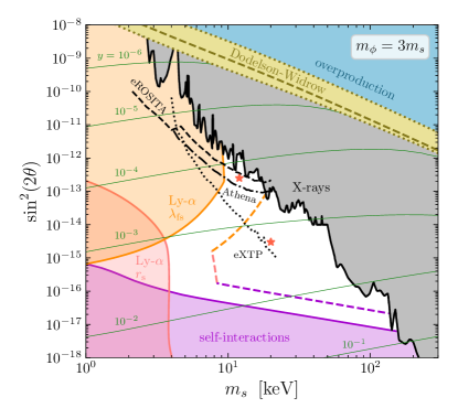
Figure 3: Available parameter space in the $\sin^{2}(2\theta)-m_{s}$ plane, for $m_{\phi}=3m_{s}$. The Yukawa coupling $y$ (green lines) is chosen such that the correct DM relic abundance is achieved everywhere below the DW line. Present and projected bounds from X-rays (filled gray and black lines), Lyman-$\alpha$ (orange), and DM self-interactions (violet) are evaluated as described in the text. The two benchmark points BP1 and BP2 from Tab. 1, see also Fig. 2, are indicated as red stars.

In Fig. 3 we show a slice of the overall available parameter space for our setup in the $\sin^{2}(2\theta)-m_{s}$ plane, for a fixed mediator to DM mass ratio of $m_{\phi}/m_{s}=3$. For every point in parameter space, the dark sector Yukawa coupling $y$ is chosen such that the sterile neutrinos $\nu_{s}$ make up all of DM after the era of exponential growth. In the yellow band, DW production can give the correct relic abundance, including QCD and lepton flavor uncertainties [62]; the dashed brown line corresponds to the central prediction, which is the basis for our choice of initial conditions for number and energy densities of $\nu_{s}$. In the blue region DM will be overproduced, $\Omega_{s}h^{2}>0.12$, while the other filled regions are excluded by bounds from X-ray searches (gray), Lyman-$\alpha$ observations (orange), and DM self-interactions (violet). The white region corresponds to the presently allowed parameter space.

It is worth noting that, unlike in standard freeze-out scenarios [86], later kinetic decoupling implies a shorter free-streaming length in our case because the dark sector temperature scales as $T_{\rm d}\propto T_{\nu}^{2}$ already before that point. At the same time, the sound horizon increases for later kinetic decoupling. The shape of the Lyman-$\alpha$ exclusion lines reflects this, as kinetic decoupling occurs later for larger values of $y$.

In Fig. 3 we also show the projected sensitivities of the future X-ray experiments eROSITA [73], Athena [74], and eXTP [75], which will probe smaller values of $\sin^{2}(2\theta)$. Similarly, observables related to structure formation will likely result in improved future bounds, or in fact reveal anomalies that are not easily reconcilable with a standard non-interacting cold DM scenario. While the precise reach is less clear here, we indicate with dashed orange and violet lines, respectively, the impact of choosing $\lambda_{\mathrm{fs}}<0.12\,\mathrm{Mpc}$, $r_{\mathrm{s}}<0.15\,\mathrm{Mpc}$, and $\sigma_{T}/m_{s}<0.1\,\mathrm{cm^{2}/g}$ rather than the corresponding limits described above. Overall, prospects to probe a sizable region of the presently allowed parameter space appear very promising.

Discussion.—

While an X-ray line would be the cleanest signature to claim DM discovery of the scenario suggested here, let us briefly mention other possible directions. For example, the power-spectrum of DM density perturbations at small, but only mildly non-linear, scales may be affected in a way that could be discriminated from alternative DM production scenarios by 21 cm and high-$z$ Lyman-$\alpha$ observations [87, 88, 89, 90]. Another possibility would be to search for a suppression of intense astrophysical neutrino fluxes due to $\phi$ production on $\nu_{s}$ DM at rest. We leave an investigation of these interesting avenues for future work.

We stress that the parameter space is larger than the $m_{\phi}/m_{s}=3$ slice shown in Fig. 3. Larger mass ratios, in particular, have the effect of tightening (weakening) bounds on $\lambda_{\mathrm{fs}}$ ($r_{\mathrm{s}}$), because kinetic decoupling happens earlier, and weakening self-interaction constraints; this extends the viable parameter space shown in Fig. 3 to smaller mixing angles and allows for a larger range of $m_{s}$ (cf. Fig. 2 in the Appendix). Changing the interaction structure in the dark sector, e.g. by charging the sterile neutrinos under a gauge symmetry, is a further route for model building that will not qualitatively change the new production scenario suggested here.

For completeness, we finally mention that smaller mediator masses are yet another, though qualitatively different, route worthwhile to explore. For $m_{s}<m_{\phi}<2m_{s}$ the mediator is no longer dominantly produced on-shell in transmission processes, so the cross section for transmission, $\nu_{s}\nu_{\alpha}\to\nu_{s}\nu_{s}$, scales as $y^{4}$ rather than $y^{2}$ and larger Yukawa couplings are needed in order to obtain the correct relic density. This, in turn, implies that it may only be possible to satisfy the correspondingly tighter self-interaction and Lyman-$\alpha$ constraints by adding a scalar potential for $\phi$ (because additional number-changing interactions would potentially allow an increase in the $\nu_{s}$ abundance, similar to what happens for the dashed green curve in Fig. 2, right panel, at $m_{s}/T_{\nu}\sim 0.02$). For even lighter mediators, $m_{\phi}<m_{s}$, extremely small Yukawa couplings or mixing angles would be required to prevent DM from decaying too early through $\nu_{s}\to\nu_{\alpha}\phi$ (while the decay $\nu_{s}\to 3\nu_{\alpha}$, present also in the scenario we focus on here, is automatically strongly suppressed as $\Gamma\propto y^{4}\sin^{6}\!\theta$).

Conclusions.—

Sterile neutrinos constitute an excellent DM candidate. However, X-ray observations rule out the possibility that these particles, in their simplest realization, could make up all of the observed DM. On the other hand, there has been a recent shift in focus in general DM theory, towards the possibility that DM may not just be a single, (almost) non-interacting particle. Indeed, it is perfectly conceivable that DM could belong to a more complex, secluded dark sector with its own interactions and, possibly, further particles.

By combining these ideas in the most economic way, a sterile neutrino coupled to a single additional dark sector degree of freedom allows for a qualitatively new DM production mechanism and thereby opens up ample parameter space where sterile neutrinos could still explain the entirety of DM. Excitingly, much of this parameter space is testable in the foreseeable future. In particular, our results provide a strong motivation for further pushing the sensitivity of X-ray line searches, beyond what would be expected from standard DW production.

Appendix A Appendix

Here we complement the discussion in the main text with additional, more technical information about the scenario that we study.

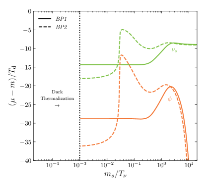
Figure 4: Evolution of the chemical potentials $\mu_{s}$ and $\mu_{\phi}$ for the benchmark points BP1 (solid lines) and BP2 (dashed lines) discussed in the main text.

Chemical potentials.—

In the main text, in Fig. 2, we showed and discussed the evolution of the dark sector temperature and number densities for the two benchmark points specified in Tab. I. Here we complement in particular the discussion of the number densities by directly showing, in Fig. 4, the evolution of the chemical potentials $\mu_{s}$ and $\mu_{\phi}$ for these benchmark points. In both cases, DW production leads to an abundance of sterile neutrinos with average momentum of the same order of magnitude as the SM neutrino temperature at the time of production, but a highly suppressed number density compared to the SM neutrino density. This leads to a large negative chemical potential $\mu_{s}=\mu_{\phi}/2\ll-T_{\mathrm{d}}$ after thermalization in the dark sector. For BP1 (solid lines) this only changes when the exponential growth of the dark sector abundance starts.

For BP2 (dashed lines) the process $\nu_{s}\nu_{s}\to\phi\phi$ becomes important around $m_{s}/T_{\nu}\sim 0.01$, which increases the abundance by effectively converting $2\nu_{s}\to 4\nu_{s}$ (see main text). This transformation of kinetic energy to rest mass decreases the temperature and very efficiently increases the chemical potential. If equilibrium with the inverse reaction $\phi\phi\to\nu_{s}\nu_{s}$ was to be established (enforcing $\mu_{\phi}=\mu_{s}$) this would eventually result in a vanishing chemical potential (since $\mu_{\phi}=2\mu_{s}$ is still enforced by $\nu_{s}\nu_{s}\leftrightarrow\phi\phi$). This point is never quite reached for BP2, however, because $\phi$ becomes Boltzmann suppressed due to $T_{\mathrm{d}}\ll m_{\phi}$ before that could happen.

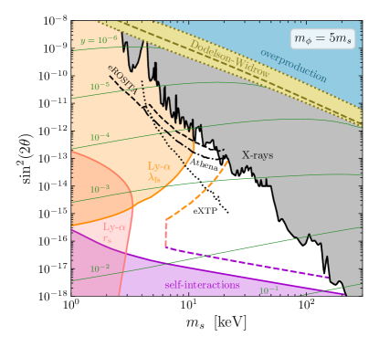
Figure 5: Same as Fig. 3 in the main text, but for $m_{\phi}=5m_{s}$.

Other mass ratios.—

In the main text, we already discussed the general impact of changing the mass ratio of $m_{\phi}/m_{s}=3$ that we chose for defining our benchmark points, as well as for illustrating the newly opened parameter space for sterile neutrino DM in Fig. 3 (of the main text). In Fig. 5 we further complement this discussion by explicitly showing the situation for $m_{\phi}/m_{s}=5$. We note that, apart from the general strengthening or weakening of constraints discussed in the main text, the Lyman-$\alpha$ forest constraint on the sound horizon first becomes stronger when increasing from very small mixing angles, against what would be expected from an earlier kinetic decoupling due to a smaller Yukawa $y$. This feature can be explained by the fact that at larger $y$ also the process $\nu_{s}\nu_{s}\to\phi\phi$ is more important, which can decrease $T_{\mathrm{d}}$ (after the decays of $\phi$) and thereby lower the speed of sound.

Collision operators.—

Here, we provide explicit expressions for the types of collision operators that we used in our analysis. As discussed in the main text, we can restrict ourselves to $1\to 2$, $2\to 1$, and $2\to 2$ interactions. We always state the collision operators $C_{n}$ for the number density of some particle $\chi\in\{\nu_{s},\,\phi\}$ from a given reaction, assuming that $\chi$ appears only once in the initial state (for an appearance in the final state the expressions need to be multiplied by $-1$). Multiple occurrences can be treated by summation over the corresponding expressions, and the total collision operator is given by the sum over all possible processes. We do not state explicitly the collision operators $C_{\rho}$ for the energy density; these can be obtained in the same way as the $C_{n}$, after multiplying the integrand with the energy $E_{\chi}$ of $\chi$.

We assume $CP$-conservation for all reactions and denote particles by numbers $i\in\{1,2,3,4\}$ ($\chi$ being one of the particles $i$), four-momenta by $\underline{\smash{p}\vphantom{T}}\vphantom{p}_{i}$, three-momenta by $\mathbb{p}_{i}$, absolute values of three-momenta by $p_{i}$, and energies by $E_{i}=\sqrt{m_{i}^{2}+p_{i}^{2}}$, where $m_{i}$ is the particle’s mass. The matrix elements in our expressions are summed over the initial- and final-state spin degrees of freedom. As the dark sector is in general not non-relativistic (or satisfies $\mu\ll-T_{\mathrm{d}}$), we fully keep spin-statistical factors and the complete Fermi-Dirac or Bose-Einstein distributions everywhere. This is particularly important for scenarios where the reaction $\nu_{s}\nu_{s}\to\phi\phi$ is relevant (roughly $y\gtrsim 4\times 10^{-4}$ in Fig. 3 in the main text, cf. dashed lines in main text Fig. 2) and can lead to a change in the final sterile neutrino abundance by more than two orders of magnitude compared to a simplified treatment assuming Boltzmann distributions and no Pauli blocking or Bose enhancement.

Starting with inverse decays, $12\to 3$, the collision operator for the number density takes the form

$$\frac{C_{n,12\to 3}}{\kappa_{12\to 3}} =\int\frac{\mathrm{d}^{3}p_{1}}{(2\pi)^{3}2E_{1}}\frac{\mathrm{d}^{3}p_{2}}{(2\pi)^{3}2E_{2}}\frac{\mathrm{d}^{3}p_{3}}{(2\pi)^{3}2E_{3}}(2\pi)^{4}$$

$$\quad\;\times\delta(\underline{\smash{p}\vphantom{T}}\vphantom{p}_{1}+\underline{\smash{p}\vphantom{T}}\vphantom{p}_{2}-\underline{\smash{p}\vphantom{T}}\vphantom{p}_{3})f_{1}f_{2}(1\pm f_{3})|\mathcal{M}_{12\to 3}|^{2}$$

$$=\frac{1}{4(2\pi)^{3}}\int_{m_{1}}^{\infty}\mathrm{d}E_{1}\int_{R_{2}}\mathrm{d}E_{3}$$

$$\quad\;\times f_{1}f_{2}(1\pm f_{3})|_{E_{3}=E_{1}+E_{2}}|\mathcal{M}_{12\to 3}|^{2}\,,$$ (6)

$$R_{2} =\{E_{2}\geq m_{2}\;|\;E_{2,-}\leq E_{2}\leq E_{2,+}\}\,,$$ (7)

$$E_{2,\pm} =\frac{1}{2m_{1}^{2}}\Bigg{(}E_{1}[m_{3}^{2}-m_{1}^{2}-m_{2}^{2}]$$ (8)

$$\quad\;\pm p_{1}\sqrt{m_{3}^{4}+(m_{1}^{2}\!-\!m_{2}^{2})^{2}-2m_{3}^{2}(m_{1}^{2}\!+\!m_{2}^{2})}\Bigg{)}\,,$$

where the symmetry factor $\kappa_{12\to 3}=1/2$ if particles 1 and 2 are identical and $\kappa_{12\to 3}=1$ if not, and the phase-space distribution functions are denoted by the $f_{i}$ (with $\pm$ denoting Bose enhancement/Pauli suppression if $3$ is a boson/fermion, analogously for other particles henceforth). Similarly, for the reverse reaction $3\to 12$, we find

$$\frac{C_{n,3\to 12}}{\kappa_{3\to 12}} =\frac{1}{4(2\pi)^{3}}\int_{m_{1}}^{\infty}\mathrm{d}E_{1}\int_{R_{2}}\mathrm{d}E_{3}$$

$$\times f_{3}(1\pm f_{2})(1\pm f_{1})|_{E_{3}=E_{1}+E_{2}}|\mathcal{M}_{12\to 3}|^{2}\,.$$ (9)

Turning to 2-to-2 reactions, with particle identifications $12\to 34$, the collision operator for the number density is given by

$$\frac{C_{n,12\to 34}}{\kappa_{12\to 34}}= \int\frac{\mathrm{d}^{3}p_{1}}{(2\pi)^{3}2E_{1}}\frac{\mathrm{d}^{3}p_{2}}{(2\pi)^{3}2E_{2}}\frac{\mathrm{d}^{3}p_{3}}{(2\pi)^{3}2E_{3}}\frac{\mathrm{d}^{3}p_{4}}{(2\pi)^{3}2E_{4}}$$

$$\times(2\pi)^{4}\delta(\underline{\smash{p}\vphantom{T}}\vphantom{p}_{1}+\underline{\smash{p}\vphantom{T}}\vphantom{p}_{2}-\underline{\smash{p}\vphantom{T}}\vphantom{p}_{3}-\underline{\smash{p}\vphantom{T}}\vphantom{p}_{4})$$

$$\times f_{1}f_{2}(1\pm f_{3})(1\pm f_{4})|\mathcal{M}_{12\to 34}|^{2}\,,$$ (10)

with the symmetry factor $\kappa_{12\to 34}$ being 1 if neither the initial-state nor the final-state particles are identical, $1/2$ if either the initial-state or the final-state particles are identical, and $1/4$ if the initial-state and the final-state particles are identical. We follow a similar approach as discussed in Ref. [91] for the Boltzmann equation at the phase-space level. After integrating over $\mathbb{p}_{4}$ using the spatial part of the $\delta$-distribution, we can write the 3-momenta in spherical coordinates as

$$\mathbb{p}_{1} =p_{1}(0,0,1)^{T}\,,$$ (11)

$$\mathbb{p}_{2} =p_{2}(\sin\beta,0,\cos\beta)^{T}$$ (12)

$$\mathbb{p}_{3} =p_{3}(\sin\theta\cos\phi,\sin\theta\sin\phi,\cos\theta)^{T}\,,$$ (13)

where $-1\leq\cos\beta\leq 1$, $0\leq\phi<2\pi$, and $-1\leq\cos\theta\leq 1$, and hence

$$\mathbb{p}_{4}^{2} =(\mathbb{p}_{1}+\mathbb{p}_{2}-\mathbb{p}_{3})^{2}$$

$$=p_{1}^{2}+p_{2}^{2}+p_{3}^{2}+2p_{1}p_{2}\cos\beta-2p_{1}p_{3}\cos\theta$$

$$\quad-2p_{2}p_{3}(\cos\beta\cos\theta+\sin\beta\sin\theta\cos\phi)\,.$$ (14)

Since the $\phi$-dependence of the entire integrand is only through $\cos\phi$, we can simply multiply by 2 and restrict the integration to $0\leq\phi\leq\pi$. In particular, the matrix element only depends on the Mandelstam variables

$$s =m_{1}^{2}+m_{2}^{2}+2E_{1}E_{2}-2p_{1}p_{2}\cos\beta\,,$$ (15)

$$t =m_{1}^{2}+m_{3}^{2}-2E_{1}E_{3}+2p_{1}p_{3}\cos\theta\,.$$ (16)

As a result, we can write the remaining $\delta$-distribution as

$$\delta(E_{1}+E_{2}-E_{3}-E_{4}|_{\mathbb{p}_{4}=\mathbb{p}_{1}+\mathbb{p}_{2}-\mathbb{p}_{3}})=$$

$$\frac{E_{1}+E_{2}-E_{3}}{p_{2}p_{3}\sin\beta\sin\theta}\delta\Big{(}\cos\phi$$

$$-\frac{1}{2p_{2}p_{3}\sin\beta\sin\theta}[m_{1}^{2}+m_{2}^{2}+m_{3}^{2}-m_{4}^{2}$$

$$+2(E_{1}E_{2}-E_{1}E_{3}-E_{2}E_{3})$$

$$-2p_{1}p_{2}\cos\beta+2p_{1}p_{3}\cos\theta+2p_{2}p_{3}\cos\beta\cos\theta]\Big{)}\,.$$ (17)

The integration over $\cos\theta$ gets restricted to $\cos\theta\in R_{\theta}$ with $R_{\theta}=\{-1\leq\cos\theta\leq 1\;|\;c_{\theta,+}\leq\cos\theta\leq c_{\theta,-}\}$ and

$$c_{\theta,\pm} =\frac{-b\pm\sqrt{b^{2}-4ac}}{2a}\,,$$ (18)

$$a =-4p_{3}^{2}[(E_{1}+E_{2})^{2}-s]\,,$$ (19)

$$b =\frac{2p_{3}}{p_{1}}[s-2E_{1}(E_{1}+E_{2})+m_{1}^{2}-m_{2}^{2}]$$

$$\quad\;\times[s-2E_{3}(E_{1}+E_{2})+m_{3}^{2}-m_{4}^{2}]\,,$$ (20)

$$c =-[2E_{3}(E_{1}+E_{2})-m_{3}^{2}+m_{4}^{2}-s]^{2}$$

$$\quad\;-\frac{p_{3}^{2}}{p_{1}^{2}}(s-s_{12,-})(s-s_{12,+})\,,$$ (21)

$$s_{12/34,\pm} =m_{1/3}^{2}+m_{2/4}^{2}+2E_{1/3}E_{2/4}\pm 2p_{1/3}p_{2/4}\,,$$ (22)

with $E_{4}=E_{1}+E_{2}-E_{3}$ and $p_{4}=\sqrt{E_{4}^{2}-m_{4}^{2}}$. Performing the integration over $\phi$ we thus obtain

$$\quad\;\int\frac{\mathrm{d}^{3}p_{3}}{(2\pi)^{3}2E_{3}}\frac{\mathrm{d}^{3}p_{4}}{(2\pi)^{3}2E_{4}}(2\pi)^{4}\delta(\underline{\smash{p}\vphantom{T}}\vphantom{p}_{1}+\underline{\smash{p}\vphantom{T}}\vphantom{p}_{2}-\underline{\smash{p}\vphantom{T}}\vphantom{p}_{3}-\underline{\smash{p}\vphantom{T}}\vphantom{p}_{4})$$

$$\quad\;\times(1\pm f_{3})(1\pm f_{4})|\mathcal{M}_{12\to 34}|^{2}$$ (23)

$$=\frac{1}{(2\pi)^{2}}\int_{0}^{\infty}\mathrm{d}p_{3}\frac{p_{3}^{2}}{E_{3}}(1\pm f_{3})(1\pm f_{4})\theta(b^{2}-4ac)$$

$$\quad\;\times\int_{R_{\theta}}\frac{\mathrm{d}\cos\theta}{\sqrt{a\cos^{2}\theta+b\cos\theta+c}}|\mathcal{M}_{12\to 34}|^{2}\,,$$ (24)

where we used $2p_{2}p_{3}\sin\beta\sin\theta\sqrt{1-\cos^{2}\phi}=\sqrt{a\cos^{2}\theta+b\cos\theta+c}$ and introduced a factor of $\theta(b^{2}-4ac)$ to ensure that $c_{\theta,\pm}$ is real. After variable transformation from $\cos\beta$ to $s$, cf. Eq. (15), we thus finally arrive at

$$C_{n,12\to 34}=\frac{\kappa_{12\to 34}}{4(2\pi)^{6}}\int_{m_{1}}^{\infty}\mathrm{d}E_{1}\int_{\max(m_{2},m_{3}+m_{4}-E_{1})}^{\infty}\mathrm{d}E_{2}$$

$$\quad\times\int_{m_{3}}^{E_{1}+E_{2}-m_{4}}\mathrm{d}E_{3}\,p_{3}f_{1}f_{2}(1\pm f_{3})(1\pm f_{4})$$

$$\quad\times\int_{R_{s}}\mathrm{d}s\int_{R_{\theta}}\frac{\mathrm{d}\cos\theta}{\sqrt{a\cos^{2}\theta+b\cos\theta+c}}|\mathcal{M}_{12\to 34}|^{2}\,,$$ (25)

where $R_{s}=\{s\in\mathbb{R}\;|\;\max(s_{12,-},s_{34,-})\leq s\leq\min(s_{12,+},s_{34,+})\}$ and the integration over $\cos\theta$ can equally well be rewritten as over $t$, cf. Eq (16). We can also rearrange the integration order to

$$C_{n,12\to 34} =\frac{\kappa_{12\to 34}}{4(2\pi)^{6}}\int_{s_{\mathrm{min}}}^{\infty}\mathrm{d}s\int_{m_{1}}^{\infty}\mathrm{d}E_{1}\int_{R_{2}}\mathrm{d}E_{2}\int_{R_{3}}\mathrm{d}E_{3}$$

$$\quad\;\times p_{3}f_{1}f_{2}(1\pm f_{3})(1\pm f_{4})$$

$$\quad\;\times\int_{R_{\theta}}\frac{\mathrm{d}\cos\theta}{\sqrt{a\cos^{2}\theta+b\cos\theta+c}}|\mathcal{M}_{12\to 34}|^{2}\,,$$ (26)

where

$$s_{\mathrm{min}} =\max([m_{1}+m_{2}]^{2},[m_{3}+m_{4}]^{2})\,,$$ (27)

$$R_{2} =\{E_{2}\geq m_{2}\;|\;E_{2,-}\leq E_{2}\leq E_{2,+}\}\,,$$ (28)

$$R_{3} =\{E_{3}\geq m_{3}\;|\;E_{3,-}\leq E_{3}\leq E_{3,+}\}\,,$$ (29)

$$E_{2,\pm} =\frac{1}{2m_{1}^{2}}\Bigg{(}E_{1}[s-m_{1}^{2}-m_{2}^{2}]$$

$$\quad\;\pm p_{1}\sqrt{s^{2}+(m_{1}^{2}-m_{2}^{2})^{2}-2s(m_{1}^{2}+m_{2}^{2})}\Bigg{)}\,,$$ (30)

$$E_{3,\pm} =\frac{1}{2s}\Bigg{(}[E_{1}+E_{2}][s+m_{3}^{2}-m_{4}^{2}]\pm\sqrt{(E_{1}+E_{2})^{2}-s}$$

$$\quad\;\times\sqrt{s^{2}+(m_{3}^{2}-m_{4}^{2})^{2}-2s(m_{3}^{2}+m_{4}^{2})}\Bigg{)}\,.$$ (31)

For the matrix elements of interest in this work, see below, the integration over $\cos\theta$ can be performed analytically after a variable transformation to $x=-2\arcsin(\sqrt{(c_{\theta,-}-\cos\theta)/(c_{\theta,-}-c_{\theta,+})})$. The remaining four integrals we evaluate numerically, using Monte-Carlo methods with importance sampling.

Matrix elements.—

For completeness, we finally provide a full list of all matrix elements that are relevant for our scenario (summed over the spin degrees of freedom of all initial- and final-state particles). Note that we can safely assume $CP$-conservation for these. We start with the decay width

$$\Gamma_{\phi}=\Gamma_{\phi\to\nu_{\alpha}\nu_{\alpha}}+\Gamma_{\phi\to\nu_{\alpha}\nu_{s}}+\Gamma_{\phi\to\nu_{s}\nu_{s}}$$ (32)

of the mediator $\phi$, implicitly defining the matrix elements via the partial widths

$$\Gamma_{\phi\to\nu_{\alpha}\nu_{\alpha}} =\frac{1}{32\pi m_{\phi}}|\mathcal{M}_{\phi\to\nu_{\alpha}\nu_{\alpha}}|^{2}=\frac{1}{8\pi}y^{2}\sin^{4}\!\theta\,m_{\phi}\,,$$ (33)

$$\Gamma_{\phi\to\nu_{\alpha}\nu_{s}} =\frac{m_{\phi}^{2}-m_{s}^{2}}{16\pi m_{\phi}^{3}}|\mathcal{M}_{\phi\to\nu_{\alpha}\nu_{s}}|^{2}\Theta(m_{\phi}-m_{s})$$ (34)

$$=\frac{1}{8\pi}y^{2}\sin^{2}\theta\cos^{2}\theta\,\frac{(m_{\phi}^{2}-m_{s}^{2})^{2}}{m_{\phi}^{3}}\Theta(m_{\phi}-m_{s})\,,$$

$$\Gamma_{\phi\to\nu_{s}\nu_{s}} =\frac{(m_{\phi}^{2}-4m_{s}^{2})^{1/2}}{32\pi m_{\phi}^{2}}|\mathcal{M}_{\phi\to\nu_{s}\nu_{s}}|^{2}\Theta(m_{\phi}-2m_{s})$$

$$=\frac{1}{8\pi}y^{2}\cos^{4}\theta\,\frac{(m_{\phi}^{2}-4m_{s}^{2})^{3/2}}{m_{\phi}^{2}}\Theta(m_{\phi}-2m_{s})\,.$$ (35)

We note that, typically, $\Gamma_{\phi}\simeq\Gamma_{\phi\to\nu_{s}\nu_{s}}$ as $\sin\theta\ll 1$.

Turning to $2\to 2$ processes, we find

$$|\mathcal{M}_{\nu_{s}\nu_{s}\to\phi\phi}|^{2}=2y^{4}\cos^{8}\theta\times\frac{(s+2t-2m_{\phi}^{2}-2m_{s}^{2})(-m_{s}^{4}-m_{\phi}^{4}-m_{s}(2m_{\phi}^{2}-s-2t)+2m_{\phi}^{2}t-t(s+t))}{(t-m_{s}^{2})^{2}(u-m_{s}^{2})^{2}}\,.$$ (36)

for the matrix element of $\nu_{s}\nu_{s}\to\phi\phi$, and for $\nu_{1}\nu_{2}\to\nu_{3}\nu_{4}$ – with 1, 2, 3, and 4 being $s$ or $\alpha$ – we have

$$|\mathcal{M}_{\nu_{1}\nu_{2}\to\nu_{3}\nu_{4}}|^{2}=4\tilde{y}^{2}\Bigg{[}\frac{((m_{1}+m_{2})^{2}-s)((m_{3}+m_{4})^{2}-s)}{(s-m_{\phi}^{2})^{2}+m_{\phi}^{2}\Gamma_{\phi}^{2}}+\frac{((m_{1}+m_{3})^{2}-t)((m_{2}+m_{4})^{2}-t)}{(t-m_{\phi}^{2})^{2}+m_{\phi}^{2}\Gamma_{\phi}^{2}}$$

$$+\frac{((m_{1}+m_{4})^{2}-u)((m_{2}+m_{3})^{2}-u)}{(u-m_{\phi}^{2})^{2}+m_{\phi}^{2}\Gamma_{\phi}^{2}}-\frac{(s-m_{\phi}^{2})(t-m_{\phi}^{2})+m_{\phi}^{2}\Gamma_{\phi}^{2}}{[(s-m_{\phi}^{2})^{2}+m_{\phi}^{2}\Gamma_{\phi}^{2}][(t-m_{\phi}^{2})^{2}+m_{\phi}^{2}\Gamma_{\phi}^{2}]}$$

$$\times[m_{1}^{3}m_{4}+m_{1}^{2}m_{4}(m_{2}+m_{3}+m_{4})+m_{2}m_{3}(m_{2}^{2}+(m_{2}+m_{3})(m_{3}+m_{4}))-m_{3}(m_{2}+m_{4})s-(m_{2}(m_{3}+m_{4})+s)t$$

$$+m_{1}(m_{2}^{2}m_{3}+m_{4}(m_{4}(m_{3}+m_{4})-s)+m_{2}((m_{3}+m_{4})^{2}-s)-(m_{3}+m_{4})t)]$$

$$-\frac{(s-m_{\phi}^{2})(u-m_{\phi}^{2})+m_{\phi}^{2}\Gamma_{\phi}^{2}}{[(s-m_{\phi}^{2})^{2}+m_{\phi}^{2}\Gamma_{\phi}^{2}][(u-m_{\phi}^{2})^{2}+m_{\phi}^{2}\Gamma_{\phi}^{2}]}[m_{1}^{3}m_{3}+m_{1}^{2}m_{3}(m_{2}+m_{3}+m_{4})+m_{2}m_{4}(m_{2}^{2}+(m_{2}+m_{4})(m_{3}+m_{4}))$$

$$-(m_{2}+m_{3})m_{4}s-(m_{2}(m_{3}+m_{4})+s)u$$

$$+m_{1}(m_{2}^{2}m_{4}+m_{3}(m_{3}(m_{3}+m_{4})-s)+m_{2}((m_{3}+m_{4})^{2}-s)-(m_{3}+m_{4})u)]$$

$$-\frac{(t-m_{\phi}^{2})(u-m_{\phi}^{2})+m_{\phi}^{2}\Gamma_{\phi}^{2}}{[(t-m_{\phi}^{2})^{2}+m_{\phi}^{2}\Gamma_{\phi}^{2}][(u-m_{\phi}^{2})^{2}+m_{\phi}^{2}\Gamma_{\phi}^{2}]}[m_{1}^{3}m_{2}+m_{1}^{2}m_{2}(m_{2}+m_{3}+m_{4})+m_{3}m_{4}(m_{4}^{2}+(m_{2}+m_{3})(m_{3}+m_{4}))$$

$$-m_{4}(m_{2}+m_{3})t-(m_{3}(m_{2}+m_{4})+t)u$$

$$+m_{1}(m_{2}^{3}+m_{2}^{2}(m_{3}+m_{4})+m_{3}m_{4}(m_{3}+m_{4})-m_{3}t+m_{2}(2m_{3}m_{4}-t-u)-m_{4}u)]\Bigg{]}\,.$$ (37)

Here the Mandelstam variables $s$, $t$, and $u$ follow the standard definition, and $\tilde{y}^{2}=y^{4}\cos^{8}\theta$ for elastic scattering $\nu_{s}\nu_{s}\to\nu_{s}\nu_{s}$, $\tilde{y}^{2}=y^{4}\cos^{4}\theta\sin^{4}\theta$ for the transformation process $\nu_{s}\nu_{\alpha}\to\nu_{s}\nu_{s}$, and $\tilde{y}^{2}=y^{4}\cos^{4}\theta\sin^{4}\theta$ for freeze-in $\nu_{\alpha}\nu_{\alpha}\to\nu_{s}\nu_{s}$ (which can generally be neglected).

In the main text, we have stressed that dark sector thermalization and the phase of exponential growth are mostly due to the 3-body interactions $\nu_{s}\nu_{s}\leftrightarrow\phi$ and $\nu_{s}\nu_{\alpha}\to\phi$. These scale as $y^{2}$ and are equal to the on-shell contribution to the $s$-channel part of $\nu_{1}\nu_{2}\to\nu_{3}\nu_{4}$, cf. the first term in Eq. (37). From the full expression of the matrix element, see also Fig. 1 in the main text, it is however evident that there are also contributions from $t/u$-channel diagrams, as well as $s$-channel contributions with an off-shell mediator. The processes $\nu_{s}\nu_{s}\to\nu_{s}\nu_{s}$ and $\nu_{s}\nu_{\alpha}\to\nu_{s}\nu_{s}$ thus have interaction rates scaling as $y^{4}$ far away from the $s$-channel resonance. Since $\nu_{s}\nu_{\alpha}\to\phi$ is at most barely larger than the Hubble rate (cf. left panel of Fig. 2 in the main text), the additional suppression by $y^{2}$ causes the off-shell contribution to $\nu_{s}\nu_{\alpha}\to\nu_{s}\nu_{s}$ to be negligible.

As also discussed in the main text, it is sufficient to solve the Boltzmann equations for $\tilde{n}=n_{s}+2n_{\phi}$ and $\rho=\rho_{s}+\rho_{\phi}$ since $\nu_{s}\nu_{s}\leftrightarrow\phi$ thermalizes the dark sector. Self-scatterings $\nu_{s}\nu_{s}\leftrightarrow\nu_{s}\nu_{s}$ do not change number or energy density, i.e. their contribution to the corresponding collision operators is zero. Similarly, $\nu_{s}\nu_{s}\leftrightarrow\phi$ does not change $\tilde{n}$ or $\rho$ and does not need to be calculated for the evolution. Note however that the full process $\nu_{s}\nu_{s}\to\nu_{s}\nu_{s}$ is relevant for kinetic decoupling, which can occur after $\phi$ becomes highly Boltzmann suppressed at $T_{\mathrm{d}}\ll m_{\phi}$.

References

- Minkowski [1977] P. Minkowski, at a Rate of One Out of Muon Decays?, Phys. Lett. B 67, 421 (1977).
- Yanagida [1979] T. Yanagida, Horizontal gauge symmetry and masses of neutrinos, in Proceedings of the Workshop on the Unified Theory and the Baryon Number in the Universe, edited by O. Sawada and A. Sugamoto (KEK, Tsukuba, Japan, 1979) p. 95.
- Glashow [1980] S. L. Glashow, The future of elementary particle physics, in Proceedings of the 1979 Cargèse Summer Institute on Quarks and Leptons, edited by M. Lévy, J.-L. Basdevant, D. Speiser, J. Weyers, R. Gastmans, and M. Jacob (Plenum Press, New York, 1980) pp. 687–713.
- Gell-Mann et al. [1979] M. Gell-Mann, P. Ramond, and R. Slansky, Complex spinors and unified theories, in Supergravity, edited by P. van Nieuwenhuizen and D. Z. Freedman (North Holland, Amsterdam, 1979) p. 315, arXiv:1306.4669 [hep-th] .
- Mohapatra and Senjanović [1980] R. N. Mohapatra and G. Senjanović, Neutrino Mass and Spontaneous Parity Nonconservation, Phys. Rev. Lett. 44, 912 (1980).
- Sajjad Athar et al. [2022] M. Sajjad Athar et al., Status and perspectives of neutrino physics, Prog. Part. Nucl. Phys. 124, 103947 (2022), arXiv:2111.07586 [hep-ph] .
- Boyarsky et al. [2019] A. Boyarsky, M. Drewes, T. Lasserre, S. Mertens, and O. Ruchayskiy, Sterile neutrino Dark Matter, Prog. Part. Nucl. Phys. 104, 1 (2019), arXiv:1807.07938 [hep-ph] .
- Abazajian et al. [2001] K. Abazajian, G. M. Fuller, and W. H. Tucker, Direct detection of warm dark matter in the X-ray, Astrophys. J. 562, 593 (2001), arXiv:astro-ph/0106002 .
- Gerbino et al. [2022] M. Gerbino et al., Synergy between cosmological and laboratory searches in neutrino physics: a white paper, (2022), arXiv:2203.07377 [hep-ph] .
- Bulbul et al. [2014] E. Bulbul, M. Markevitch, A. Foster, R. K. Smith, M. Loewenstein, and S. W. Randall, Detection of An Unidentified Emission Line in the Stacked X-ray spectrum of Galaxy Clusters, Astrophys. J. 789, 13 (2014), arXiv:1402.2301 [astro-ph.CO] .
- Boyarsky et al. [2014] A. Boyarsky, O. Ruchayskiy, D. Iakubovskyi, and J. Franse, Unidentified Line in X-Ray Spectra of the Andromeda Galaxy and Perseus Galaxy Cluster, Phys. Rev. Lett. 113, 251301 (2014), arXiv:1402.4119 [astro-ph.CO] .
- Dodelson and Widrow [1994] S. Dodelson and L. M. Widrow, Sterile-neutrinos as dark matter, Phys. Rev. Lett. 72, 17 (1994), arXiv:hep-ph/9303287 .
- Abazajian [2017] K. N. Abazajian, Sterile neutrinos in cosmology, Phys. Rept. 711-712, 1 (2017), arXiv:1705.01837 [hep-ph] .
- Shi and Fuller [1999] X. Shi and G. M. Fuller, New Dark Matter Candidate: Nonthermal Sterile Neutrinos, Phys. Rev. Lett. 82, 2832 (1999), arXiv:astro-ph/9810076 .
- Shaposhnikov and Tkachev [2006] M. Shaposhnikov and I. Tkachev, The nuMSM, inflation, and dark matter, Phys. Lett. B 639, 414 (2006), arXiv:hep-ph/0604236 .
- Kusenko [2006] A. Kusenko, Sterile neutrinos, dark matter, and the pulsar velocities in models with a Higgs singlet, Phys. Rev. Lett. 97, 241301 (2006), arXiv:hep-ph/0609081 .
- Petraki and Kusenko [2008] K. Petraki and A. Kusenko, Dark-matter sterile neutrinos in models with a gauge singlet in the Higgs sector, Phys. Rev. D 77, 065014 (2008), arXiv:0711.4646 [hep-ph] .
- Roland et al. [2015] S. B. Roland, B. Shakya, and J. D. Wells, Neutrino Masses and Sterile Neutrino Dark Matter from the PeV Scale, Phys. Rev. D 92, 113009 (2015), arXiv:1412.4791 [hep-ph] .
- Merle and Totzauer [2015] A. Merle and M. Totzauer, keV Sterile Neutrino Dark Matter from Singlet Scalar Decays: Basic Concepts and Subtle Features, JCAP 06 (2015), 011, arXiv:1502.01011 [hep-ph] .
- König et al. [2016] J. König, A. Merle, and M. Totzauer, keV Sterile Neutrino Dark Matter from Singlet Scalar Decays: The Most General Case, JCAP 11 (2016), 038, arXiv:1609.01289 [hep-ph] .
- Bezrukov et al. [2010] F. Bezrukov, H. Hettmansperger, and M. Lindner, keV sterile neutrino Dark Matter in gauge extensions of the Standard Model, Phys. Rev. D 81, 085032 (2010), arXiv:0912.4415 [hep-ph] .
- Kusenko et al. [2010] A. Kusenko, F. Takahashi, and T. T. Yanagida, Dark Matter from Split Seesaw, Phys. Lett. B 693, 144 (2010), arXiv:1006.1731 [hep-ph] .
- Dror et al. [2020] J. A. Dror, D. Dunsky, L. J. Hall, and K. Harigaya, Sterile Neutrino Dark Matter in Left-Right Theories, JHEP 07 (2020), 168, arXiv:2004.09511 [hep-ph] .
- De Gouvêa et al. [2020] A. De Gouvêa, M. Sen, W. Tangarife, and Y. Zhang, Dodelson-Widrow Mechanism in the Presence of Self-Interacting Neutrinos, Phys. Rev. Lett. 124, 081802 (2020), arXiv:1910.04901 [hep-ph] .
- Kelly et al. [2020] K. J. Kelly, M. Sen, W. Tangarife, and Y. Zhang, Origin of sterile neutrino dark matter via secret neutrino interactions with vector bosons, Phys. Rev. D 101, 115031 (2020), arXiv:2005.03681 [hep-ph] .
- Chichiri et al. [2022] C. Chichiri, G. B. Gelmini, P. Lu, and V. Takhistov, Cosmological dependence of sterile neutrino dark matter with self-interacting neutrinos, JCAP 09 (2022), 036, arXiv:2111.04087 [hep-ph] .
- Benso et al. [2022] C. Benso, W. Rodejohann, M. Sen, and A. U. Ramachandran, Sterile neutrino dark matter production in presence of nonstandard neutrino self-interactions: An EFT approach, Phys. Rev. D 105, 055016 (2022), arXiv:2112.00758 [hep-ph] .
- Hansen and Vogl [2017] R. S. L. Hansen and S. Vogl, Thermalizing sterile neutrino dark matter, Phys. Rev. Lett. 119, 251305 (2017), arXiv:1706.02707 [hep-ph] .
- Bringmann et al. [2021a] T. Bringmann, P. F. Depta, M. Hufnagel, J. T. Ruderman, and K. Schmidt-Hoberg, Dark Matter from Exponential Growth, Phys. Rev. Lett. 127, 191802 (2021a), arXiv:2103.16572 [hep-ph] .
- Hryczuk and Laletin [2021] A. Hryczuk and M. Laletin, Dark matter freeze-in from semi-production, JHEP 06 (2021), 026, arXiv:2104.05684 [hep-ph] .
- Hall et al. [2010] L. J. Hall, K. Jedamzik, J. March-Russell, and S. M. West, Freeze-In Production of FIMP Dark Matter, JHEP 03 (2010), 080, arXiv:0911.1120 [hep-ph] .
- Pospelov et al. [2008] M. Pospelov, A. Ritz, and M. B. Voloshin, Secluded WIMP Dark Matter, Phys. Lett. B 662, 53 (2008), arXiv:0711.4866 [hep-ph] .
- Feng et al. [2008] J. L. Feng, H. Tu, and H.-B. Yu, Thermal Relics in Hidden Sectors, JCAP 10 (2008), 043, arXiv:0808.2318 [hep-ph] .
- Pospelov [2009] M. Pospelov, Secluded U(1) below the weak scale, Phys. Rev. D 80, 095002 (2009), arXiv:0811.1030 [hep-ph] .
- Cheung et al. [2011] C. Cheung, G. Elor, L. J. Hall, and P. Kumar, Origins of Hidden Sector Dark Matter I: Cosmology, JHEP 03 (2011), 042, arXiv:1010.0022 [hep-ph] .
- Hannestad et al. [2014] S. Hannestad, R. S. Hansen, and T. Tram, How Self-Interactions can Reconcile Sterile Neutrinos with Cosmology, Phys. Rev. Lett. 112, 031802 (2014), arXiv:1310.5926 [astro-ph.CO] .
- Dasgupta and Kopp [2014] B. Dasgupta and J. Kopp, Cosmologically Safe eV-Scale Sterile Neutrinos and Improved Dark Matter Structure, Phys. Rev. Lett. 112, 031803 (2014), arXiv:1310.6337 [hep-ph] .
- Bringmann et al. [2014] T. Bringmann, J. Hasenkamp, and J. Kersten, Tight bonds between sterile neutrinos and dark matter, JCAP 07 (2014), 042, arXiv:1312.4947 [hep-ph] .
- Ko and Tang [2014] P. Ko and Y. Tang, MDM: A Model for Sterile Neutrino and Dark Matter Reconciles Cosmological and Neutrino Oscillation Data after BICEP2, Phys. Lett. B739, 62 (2014), arXiv:1404.0236 [hep-ph] .
- Archidiacono et al. [2015] M. Archidiacono, S. Hannestad, R. S. Hansen, and T. Tram, Cosmology with self-interacting sterile neutrinos and dark matter - A pseudoscalar model, Phys. Rev. D 91, 065021 (2015), arXiv:1404.5915 [astro-ph.CO] .
- Mirizzi et al. [2015] A. Mirizzi, G. Mangano, O. Pisanti, and N. Saviano, Collisional production of sterile neutrinos via secret interactions and cosmological implications, Phys. Rev. D91, 025019 (2015), arXiv:1410.1385 [hep-ph] .
- Tang [2015] Y. Tang, More Is Different: Reconciling eV Sterile Neutrinos with Cosmological Mass Bounds, Phys. Lett. B750, 201 (2015), arXiv:1501.00059 [hep-ph] .
- Saviano et al. [2014] N. Saviano, O. Pisanti, G. Mangano, and A. Mirizzi, Unveiling secret interactions among sterile neutrinos with big-bang nucleosynthesis, Phys. Rev. D 90, 113009 (2014), arXiv:1409.1680 [astro-ph.CO] .
- Kouvaris et al. [2015] C. Kouvaris, I. M. Shoemaker, and K. Tuominen, Self-Interacting Dark Matter through the Higgs Portal, Phys. Rev. D 91, 043519 (2015), arXiv:1411.3730 [hep-ph] .
- Chu et al. [2015] X. Chu, B. Dasgupta, and J. Kopp, Sterile neutrinos with secret interactions — lasting friendship with cosmology, JCAP 10 (2015), 011, arXiv:1505.02795 [hep-ph] .
- Archidiacono et al. [2016a] M. Archidiacono, S. Hannestad, R. S. Hansen, and T. Tram, Sterile neutrinos with pseudoscalar self-interactions and cosmology, Phys. Rev. D 93, 045004 (2016a), arXiv:1508.02504 [astro-ph.CO] .
- Tabrizi and Peres [2016] Z. Tabrizi and O. L. G. Peres, Hidden interactions of sterile neutrinos as a probe for new physics, Phys. Rev. D93, 053003 (2016), arXiv:1507.06486 [hep-ph] .
- Binder et al. [2016] T. Binder, L. Covi, A. Kamada, H. Murayama, T. Takahashi, and N. Yoshida, Matter Power Spectrum in Hidden Neutrino Interacting Dark Matter Models: A Closer Look at the Collision Term, JCAP 11 (2016), 043, arXiv:1602.07624 [hep-ph] .
- Archidiacono et al. [2016b] M. Archidiacono, S. Gariazzo, C. Giunti, S. Hannestad, R. Hansen, M. Laveder, and T. Tram, Pseudoscalar—sterile neutrino interactions: reconciling the cosmos with neutrino oscillations, JCAP 08 (2016b), 067, arXiv:1606.07673 [astro-ph.CO] .
- Forastieri et al. [2017] F. Forastieri, M. Lattanzi, G. Mangano, A. Mirizzi, P. Natoli, and N. Saviano, Cosmic microwave background constraints on secret interactions among sterile neutrinos, JCAP 07 (2017), 038, arXiv:1704.00626 [astro-ph.CO] .
- Bezrukov et al. [2017] F. Bezrukov, A. Chudaykin, and D. Gorbunov, Hiding an elephant: heavy sterile neutrino with large mixing angle does not contradict cosmology, JCAP 06 (2017), 051, arXiv:1705.02184 [hep-ph] .
- Jeong et al. [2018] Y. S. Jeong, S. Palomares-Ruiz, M. H. Reno, and I. Sarcevic, Probing secret interactions of eV-scale sterile neutrinos with the diffuse supernova neutrino background, JCAP 06 (2018), 019, arXiv:1803.04541 [hep-ph] .
- Song et al. [2018] N. Song, M. C. Gonzalez-Garcia, and J. Salvado, Cosmological constraints with self-interacting sterile neutrinos, JCAP 10 (2018), 055, arXiv:1805.08218 [astro-ph.CO] .
- Chu et al. [2018] X. Chu, B. Dasgupta, M. Dentler, J. Kopp, and N. Saviano, Sterile Neutrinos with Secret Interactions – Cosmological Discord?, JCAP 11 (2018), 049, arXiv:1806.10629 [hep-ph] .
- Blennow et al. [2019] M. Blennow, E. Fernandez-Martinez, A. Olivares-Del Campo, S. Pascoli, S. Rosauro-Alcaraz, and A. V. Titov, Neutrino Portals to Dark Matter, Eur. Phys. J. C 79, 555 (2019), arXiv:1903.00006 [hep-ph] .
- Ballett et al. [2020] P. Ballett, M. Hostert, and S. Pascoli, Dark Neutrinos and a Three Portal Connection to the Standard Model, Phys. Rev. D 101, 115025 (2020), arXiv:1903.07589 [hep-ph] .
- Johns and Fuller [2019] L. Johns and G. M. Fuller, Self-interacting sterile neutrino dark matter: the heavy-mediator case, Phys. Rev. D 100, 023533 (2019), arXiv:1903.08296 [hep-ph] .
- de S. Pires [2020] C. A. de S. Pires, A cosmologically viable eV sterile neutrino model, Phys. Lett. B 800, 135135 (2020), arXiv:1908.09313 [hep-ph] .
- Archidiacono et al. [2020] M. Archidiacono, S. Gariazzo, C. Giunti, S. Hannestad, and T. Tram, Sterile neutrino self-interactions: tension and short-baseline anomalies, JCAP 12 (2020), 029, arXiv:2006.12885 [astro-ph.CO] .
- Berbig et al. [2020] M. Berbig, S. Jana, and A. Trautner, The Hubble tension and a renormalizable model of gauged neutrino self-interactions, Phys. Rev. D 102, 115008 (2020), arXiv:2004.13039 [hep-ph] .
- Corona et al. [2022] M. A. Corona, R. Murgia, M. Cadeddu, M. Archidiacono, S. Gariazzo, C. Giunti, and S. Hannestad, Pseudoscalar sterile neutrino self-interactions in light of Planck, SPT and ACT data, JCAP 06 (2022), 010, arXiv:2112.00037 [astro-ph.CO] .
- Asaka et al. [2007] T. Asaka, M. Laine, and M. Shaposhnikov, Lightest sterile neutrino abundance within the nuMSM, JHEP 01 (2007), 091, [Erratum: JHEP 02 (2015), 028], arXiv:hep-ph/0612182 .
- Bringmann et al. [2021b] T. Bringmann, P. F. Depta, M. Hufnagel, and K. Schmidt-Hoberg, Precise dark matter relic abundance in decoupled sectors, Phys. Lett. B 817, 136341 (2021b), arXiv:2007.03696 [hep-ph] .
- Aghanim et al. [2020] N. Aghanim et al. (Planck), Planck 2018 results. VI. Cosmological parameters, Astron. Astrophys. 641, A6 (2020), [Erratum: Astron. Astrophys. 652, C4 (2021)], arXiv:1807.06209 [astro-ph.CO] .
- Mondino et al. [2021] C. Mondino, M. Pospelov, J. T. Ruderman, and O. Slone, Dark Higgs Dark Matter, Phys. Rev. D 103, 035027 (2021), arXiv:2005.02397 [hep-ph] .
- March-Russell et al. [2020] J. March-Russell, H. Tillim, and S. M. West, Reproductive freeze-in of self-interacting dark matter, Phys. Rev. D 102, 083018 (2020), arXiv:2007.14688 [astro-ph.CO] .
- Horiuchi et al. [2014] S. Horiuchi, P. J. Humphrey, J. Onorbe, K. N. Abazajian, M. Kaplinghat, and S. Garrison-Kimmel, Sterile neutrino dark matter bounds from galaxies of the Local Group, Phys. Rev. D 89, 025017 (2014), arXiv:1311.0282 [astro-ph.CO] .
- Malyshev et al. [2014] D. Malyshev, A. Neronov, and D. Eckert, Constraints on 3.55 keV line emission from stacked observations of dwarf spheroidal galaxies, Phys. Rev. D 90, 103506 (2014), arXiv:1408.3531 [astro-ph.HE] .
- Foster et al. [2021] J. W. Foster, M. Kongsore, C. Dessert, Y. Park, N. L. Rodd, K. Cranmer, and B. R. Safdi, Deep Search for Decaying Dark Matter with XMM-Newton Blank-Sky Observations, Phys. Rev. Lett. 127, 051101 (2021), arXiv:2102.02207 [astro-ph.CO] .
- Sicilian et al. [2020] D. Sicilian, N. Cappelluti, E. Bulbul, F. Civano, M. Moscetti, and C. S. Reynolds, Probing the Milky Way’s Dark Matter Halo for the 3.5 keV Line, Astrophys. J. 905, 146 (2020), arXiv:2008.02283 [astro-ph.HE] .
- Roach et al. [2020] B. M. Roach, K. C. Y. Ng, K. Perez, J. F. Beacom, S. Horiuchi, R. Krivonos, and D. R. Wik, NuSTAR Tests of Sterile-Neutrino Dark Matter: New Galactic Bulge Observations and Combined Impact, Phys. Rev. D 101, 103011 (2020), arXiv:1908.09037 [astro-ph.HE] .
- Boyarsky et al. [2008] A. Boyarsky, D. Malyshev, A. Neronov, and O. Ruchayskiy, Constraining DM properties with SPI, Mon. Not. Roy. Astron. Soc. 387, 1345 (2008), arXiv:0710.4922 [astro-ph] .
- Dekker et al. [2021] A. Dekker, E. Peerbooms, F. Zimmer, K. C. Y. Ng, and S. Ando, Searches for sterile neutrinos and axionlike particles from the Galactic halo with eROSITA, Phys. Rev. D 104, 023021 (2021), arXiv:2103.13241 [astro-ph.HE] .
- Ando et al. [2021] S. Ando et al., Decaying dark matter in dwarf spheroidal galaxies: Prospects for x-ray and gamma-ray telescopes, Phys. Rev. D 104, 023022 (2021), arXiv:2103.13242 [astro-ph.HE] .
- Malyshev et al. [2020] D. Malyshev, C. Thorpe-Morgan, A. Santangelo, J. Jochum, and S.-N. Zhang, perspectives for the MSM sterile neutrino dark matter model, Phys. Rev. D 101, 123009 (2020), arXiv:2001.07014 [astro-ph.HE] .
- Hryczuk and Laletin [2022] A. Hryczuk and M. Laletin, Impact of dark matter self-scattering on its relic abundance, Phys. Rev. D 106, 023007 (2022), arXiv:2204.07078 [hep-ph] .
- Egana-Ugrinovic et al. [2021] D. Egana-Ugrinovic, R. Essig, D. Gift, and M. LoVerde, The Cosmological Evolution of Self-interacting Dark Matter, JCAP 05 (2021), 013, arXiv:2102.06215 [astro-ph.CO] .
- Vogelsberger et al. [2016] M. Vogelsberger, J. Zavala, F.-Y. Cyr-Racine, C. Pfrommer, T. Bringmann, and K. Sigurdson, ETHOS – an effective theory of structure formation: dark matter physics as a possible explanation of the small-scale CDM problems, Mon. Not. Roy. Astron. Soc. 460, 1399 (2016), arXiv:1512.05349 [astro-ph.CO] .
- Garzilli et al. [2021] A. Garzilli, A. Magalich, O. Ruchayskiy, and A. Boyarsky, How to constrain warm dark matter with the Lyman- forest, Mon. Not. Roy. Astron. Soc. 502, 2356 (2021), arXiv:1912.09397 [astro-ph.CO] .
- Palanque-Delabrouille et al. [2020] N. Palanque-Delabrouille, C. Yèche, N. Schöneberg, J. Lesgourgues, M. Walther, S. Chabanier, and E. Armengaud, Hints, neutrino bounds and WDM constraints from SDSS DR14 Lyman- and Planck full-survey data, JCAP 04 (2020), 038, arXiv:1911.09073 [astro-ph.CO] .
- Tulin and Yu [2018] S. Tulin and H.-B. Yu, Dark Matter Self-interactions and Small Scale Structure, Phys. Rept. 730, 1 (2018), arXiv:1705.02358 [hep-ph] .
- Kahlhoefer et al. [2014] F. Kahlhoefer, K. Schmidt-Hoberg, M. T. Frandsen, and S. Sarkar, Colliding clusters and dark matter self-interactions, Mon. Not. Roy. Astron. Soc. 437, 2865 (2014), arXiv:1308.3419 [astro-ph.CO] .
- Kaplinghat et al. [2016] M. Kaplinghat, S. Tulin, and H.-B. Yu, Dark Matter Halos as Particle Colliders: Unified Solution to Small-Scale Structure Puzzles from Dwarfs to Clusters, Phys. Rev. Lett. 116, 041302 (2016), arXiv:1508.03339 [astro-ph.CO] .
- Andrade et al. [2021] K. E. Andrade, J. Fuson, S. Gad-Nasr, D. Kong, Q. Minor, M. G. Roberts, and M. Kaplinghat, A stringent upper limit on dark matter self-interaction cross-section from cluster strong lensing, Mon. Not. Roy. Astron. Soc. 510, 54 (2021), arXiv:2012.06611 [astro-ph.CO] .
- Bondarenko et al. [2018] K. Bondarenko, A. Boyarsky, T. Bringmann, and A. Sokolenko, Constraining self-interacting dark matter with scaling laws of observed halo surface densities, JCAP 04 (2018), 049, arXiv:1712.06602 [astro-ph.CO] .
- Bringmann [2009] T. Bringmann, Particle Models and the Small-Scale Structure of Dark Matter, New J. Phys. 11, 105027 (2009), arXiv:0903.0189 [astro-ph.CO] .
- Bose et al. [2019] S. Bose, M. Vogelsberger, J. Zavala, C. Pfrommer, F.-Y. Cyr-Racine, S. Bohr, and T. Bringmann, ETHOS – an Effective Theory of Structure Formation: detecting dark matter interactions through the Lyman- forest, Mon. Not. Roy. Astron. Soc. 487, 522 (2019), arXiv:1811.10630 [astro-ph.CO] .
- Muñoz et al. [2020] J. B. Muñoz, C. Dvorkin, and F.-Y. Cyr-Racine, Probing the Small-Scale Matter Power Spectrum with Large-Scale 21-cm Data, Phys. Rev. D 101, 063526 (2020), arXiv:1911.11144 [astro-ph.CO] .
- Muñoz et al. [2021] J. B. Muñoz, S. Bohr, F.-Y. Cyr-Racine, J. Zavala, and M. Vogelsberger, ETHOS - an effective theory of structure formation: Impact of dark acoustic oscillations on cosmic dawn, Phys. Rev. D 103, 043512 (2021), arXiv:2011.05333 [astro-ph.CO] .
- Schaeffer and Schneider [2021] T. Schaeffer and A. Schneider, Dark acoustic oscillations: imprints on the matter power spectrum and the halo mass function, Mon. Not. Roy. Astron. Soc. 504, 3773 (2021), arXiv:2101.12229 [astro-ph.CO] .
- Ala-Mattinen et al. [2022] K. Ala-Mattinen, M. Heikinheimo, K. Kainulainen, and K. Tuominen, Momentum distributions of cosmic relics: Improved analysis, Phys. Rev. D 105, 123005 (2022), arXiv:2201.06456 [hep-ph] .