Tyler’s and Maronna’s M-estimators: Non-Asymptotic Concentration Results

Abstract

Tyler’s and Maronna’s M-estimators, as well as their regularized variants, are popular robust methods to estimate the scatter or covariance matrix of a multivariate distribution. In this work, we study the non-asymptotic behavior of these estimators, for data sampled from a distribution that satisfies one of the following properties: 1) independent sub-Gaussian entries, up to a linear transformation; 2) log-concave distributions; 3) distributions satisfying a convex concentration property. Our main contribution is the derivation of tight non-asymptotic concentration bounds of these M-estimators around a suitably scaled version of the data sample covariance matrix. Prior to our work, non-asymptotic bounds were derived only for Elliptical and Gaussian distributions. Our proof uses a variety of tools from non asymptotic random matrix theory and high dimensional geometry. Finally, we illustrate the utility of our results on two examples of practical interest: sparse covariance and sparse precision matrix estimation.

1 Introduction

Let ${\bf x}_{1},\ldots,{\bf x}_{n}$ be $n$ i.i.d. samples from a $p$-dimensional random variable $X$. The $p\times p$ covariance matrix $\Sigma$ of $X$ is a central quantity of interest in multiple applications [5, 59]. In the classical regime with $n\gg p$, if the random variable $X$ is not heavily tailed and there are no outliers, the empirical covariance matrix yields a relatively accurate estimator for $\Sigma$.

To deal with heavy tails and potential outliers, several robust estimators were proposed and studied theoretically. Two popular procedures, applicable when $p<n$, include Maronna’s and Tyler’s M-estimators [51, 74]. Regularized variants, applicable also when $p>n$, were also proposed and studied [1, 61, 22, 63]. These estimators have found use in multiple applications, ranging from signal processing and radar detection to finance, see for example [24, 63, 61]. We remark that in addition to the above, many other robust covariance estimators have been proposed and analyzed, see for example [38, 77, 30, 52, 19, 20, 40, 56, 55, 28] and references therein.

In this work we study the properties of Tyler’s and Maronna’s M-estimators under several families of multivariate distributions. Our analysis is non-asymptotic and generalizes previous results, which were either asymptotic or limited to elliptical distributions. Before presenting our results, we first briefly describe these estimators and related prior work. For simplicity, we describe the estimators assuming $X$ has zero mean, and discuss how to relax this assumption later on.

Maronna’s M-estimator (ME)

One of the first proposals for a robust covariance estimator, introduced by Maronna [51], is defined as follows. Let $u:[0,\infty)\to(0,\infty)$ be a function that is strictly positive, non-increasing, continuous, and such that the accompanying function $\phi(x)=xu(x)$ is non-decreasing and bounded. Then, for $n\geq p$, Maronna’s M-estimator (if exists) is a solution to the non-linear matrix equation

$$\hat{\Sigma}_{\mbox{\tiny{Mar}}}=\frac{1}{n}\sum_{i=1}^{n}w^{\mbox{\tiny{Mar}}}_{i}{\bf x}_{i}{\bf x}_{i}^{\top}\,,\quad\textrm{where }\quad w^{\mbox{\tiny{Mar}}}_{i}=u\left(\frac{1}{p}{\bf x}_{i}^{\top}\hat{\Sigma}_{\mbox{\tiny{Mar}}}^{-1}{\bf x}_{i}\right)\,.$$ (1)

Maronna [51] proved that under certain deterministic conditions on the samples ${\bf x}_{i}$, Eq. (1) has a unique solution. Couillet et al. [25] considered a high dimensional asymptotic framework, wherein $n,p\to\infty$ with their ratio converging to a constant. Assuming that $X$ has i.i.d. entries with sufficiently many finite moments, and that $\phi_{\infty}:=\sup_{x}\phi(x)>1$, they proved that Eq. (1) has a unique solution with probability tending to one.

Maronna’s regularized M-estimator (MRE)

For $p>n$, Ollila and Tyler [61] proposed the following generalization of Maronna’s M-estimator: For regularization parameter $\alpha>0$,

$$\hat{\Sigma}_{\mbox{\tiny{MRE}}}=\frac{1}{1+\alpha}\frac{1}{n}\sum_{i=1}^{n}w^{\mbox{\tiny{MRE}}}_{i}{\bf x}_{i}{\bf x}_{i}^{\top}+\frac{\alpha}{1+\alpha}\mathrm{I}_{p\times p}\,,\quad\textrm{where }\quad w^{\mbox{\tiny{MRE}}}_{i}=u\left(\frac{1}{p}{\bf x}_{i}^{\top}\hat{\Sigma}_{\mbox{\tiny{MRE}}}^{-1}{\bf x}_{i}\right)\,.$$ (2)

As proven in [61, Theorem 1], for any ${\bf x}_{1},\ldots,{\bf x}_{n}$ and $\alpha>0$, Eq. (2) has a unique solution.

Tyler’s M-estimator (TE)

Introduced by Tyler in [74], TE is defined as the solution (if exists) of

$$\hat{\Sigma}_{\mbox{\tiny{Tyl}}}=\frac{1}{n}\sum_{i=1}^{n}w^{\mbox{\tiny{Tyl}}}_{i}{\bf x}_{i}{\bf x}_{i}^{\top},\quad\textrm{where}\quad w^{\mbox{\tiny{Tyl}}}_{i}=\left(\frac{1}{p}{\bf x}^{\top}_{i}\hat{\Sigma}_{\mbox{\tiny{Tyl}}}^{-1}{\bf x}_{i}\right)^{-1},\quad\textrm{and subject to }\quad\textrm{Tr}(\hat{\Sigma}_{\mbox{\tiny{Tyl}}})=p\,.$$ (3)

While Tyler’s estimator may seem like a special case of Maronna’s with $u(x)=1/x$, this is not so since $u(\cdot)$ is singular at $x=0$. For $n>p$, Kent and Tyler [42, Theorems 1 and 2] proved existence and uniqueness of TE under the condition that any linear subspace of $\mathbb{R}^{p}$ of dimension $1\leq d\leq p-1$ contains less than $nd/p$ samples. For i.i.d. samples from a random vector $X$ with a proper density in $\mathbb{R}^{p}$, this condition is satisfied with probability one.

Tyler’s regularized M-estimator (TRE)

Similarly to ME, Tyler’s M-estimator does not exist for $p>n.$ In recent years, several regularized variants were proposed [1, 22, 63, 72, 61]. We focus on the estimator proposed in [63]. Given a regularization parameter $\alpha>0$, it is defined by

$$\hat{\Sigma}_{\mbox{\tiny{TRE}}}=\frac{1}{1+\alpha}\frac{1}{n}\sum_{i=1}^{n}w^{\mbox{\tiny{TRE}}}_{i}{\bf x}_{i}{\bf x}_{i}^{\top}+\frac{\alpha}{1+\alpha}\mathrm{I}_{p\times p}\,,\quad\textrm{and }\quad w^{\mbox{\tiny{TRE}}}_{i}=\left(\frac{1}{p}{\bf x}_{i}^{\top}\hat{\Sigma}_{\mbox{\tiny{TRE}}}^{-1}{\bf x}_{i}\right)^{-1}\,.$$ (4)

By [61, Theorem 2], when $\alpha>p-1$, Eq. (4) always admits a unique solution. When $\alpha\leq p-1$, [61, Theorem 3] gave a deterministic sufficient and almost necessary condition for existence and uniqueness; for ${\bf x}_{1},\ldots,{\bf x}_{n}$ in general position, the condition holds for $\alpha>\max\left\{0,\frac{p}{n}-1\right\}$. When $X$ has a density, this condition appeared earlier in [63].

Prior work

Maronna’s and Tyler’s M-estimators and their variants, have been studied extensively, with a particular focus under elliptical distributions; see [76, 70, 1, 61, 22, 63, 77, 25, 26, 24, 60, 79, 33, 42, 58, 6, 62, 23]. The present paper extends several works that studied these estimators in a high-dimensional regime, where the number of samples $n$ and the dimension $p$ are both large and comparable. Couillet et al. [25] studied the asymptotic behavior of ME in the joint limit $p,n\to\infty$ with their ratio tending to a constant. Assuming that $X$ has independent entries with zero mean, unit variance and sufficiently many finite moments, they proved that after a suitable scaling, ME converges asymptotically in spectral norm to the sample covariance matrix. In [26], this analysis was extended to $X$ having an elliptical distribution with a general scatter matrix. A similar asymptotic analysis for MRE appeared in [6]. Two variants of TRE were studied in [24], assuming $X$ has an elliptical distribution. A key result of their analysis is that asymptotically, these M-estimators behave similarly to regularized sample covariance matrices with Gaussian measurements. Zhang et al. [79], studied TE assuming $X$ is Gaussian distributed with identity covariance. They showed that as $n,p\to\infty$, the limiting the spectral distribution of a properly scaled TE is a Marčenko-Pastur law. Moreover, similar to our own results in the present paper, they proved a non-asymptotic deviation bound for the weights (3), showing that they are concentrated around some particular value. Relying on their results, [33] extended the analysis to cover TRE, assuming $X$ is elliptically distributed. We remark that the proofs in [79, 33] rely on properties specific to the Gaussian and elliptical distributions, and do not extend easily to other distributions.

Another recent work is [48], which derived nonasymptotic concentration results for the Stieltjes transform of the spectral distribution of certain regularized M-estimators. In the context of this work, they derived results only for the regularized variants of Maronna’s M-estimator. Their results apply under rather broad distributional assumptions, requiring only a concentration of measure property; see also their related papers [47, 49]. In constrast, our analysis of Tyler’s M-estimators and the unregularized Maronna’s M-estimator requires an additional anti-concentration property (the small ball property) for the random vector $X$. It is an interesting question whether it is possible to derive similar results without the SBP assumption.

Our contributions

As mentioned above, most of the literature on Maronna’s and Tyler’s M-estimators has focused on asymptotic results, establishing convergence as $n,p\to\infty$ without specifying rates. Other works, that derived non-asymptotic finite-$n$ bounds, mostly considered Gaussian or elliptical distributions. This paper extends and generalizes these works in several directions. We present a non-asymptotic analysis of both Tyler’s and Marrona’s M-estimators, and their regularized variants, under three broad families of multivariate data distributions: 1) independent sub-Gaussian entries, up to a linear transformation; 2) log-concave distributions; 3) distributions satisfying a convex concentration property (CCP). Our main results are given in terms of non-asymptotic concentration bounds for the weights of the M-estimators (1)-(4) around some particular deterministic value. They imply that for these three families of distributions, Maronna’s and Tyler’s M-estimators behave similarly to a rescaled sample covariance matrix. In Section 4 we illustrate the utility of these results for two concrete examples of practical interest: sparse covariance and sparse precision matrix estimation.

2 Main results

Let ${\bf x}_{1},\ldots,{\bf x}_{n}\in\mathbb{R}^{p}$ be $n$ samples of the form

$${\bf x}_{i}=\Sigma_{p}^{1/2}\cdot{\bf y}_{i}\,,$$ (5)

where $\Sigma_{p}$ is a strictly positive $p$-by-$p$ matrix, and ${\bf y}_{1},\ldots,{\bf y}_{n}\in\mathbb{R}^{p}$ are $n$ i.i.d. realizations of a zero mean isotropic random vector $Y$, namely

$${\mathbb{E}}[Y]=\mathbf{0}\,,\quad{\mathbb{E}}[YY^{\top}]=\mathrm{I}_{p\times p}\,.$$ (6)

We assume that $Y=(Y_{1},\ldots,Y_{p})^{\top}$ is a continuous random vector, and satisfies one of the following distributional assumptions, with the precise definitions deferred to Section 3:

1. [SG-IND]: The coordinates of $Y$ are independent, sub-Gaussian (Definition 1) and have a bounded density. The constant $K>0$ denotes a uniform bound on sub-Gaussian constants, and $C_{0}>0$ a bound on the densities.

2. [CCP-SBP]: $Y$ satisfies the convex concentration property (CCP) with constant $K>0$ and also the small-ball property (SBP) with constant $C_{0}>0$ (Definition 3).

3. [LC]: $Y$ has a log-concave distribution (Definition 4).

Remark 1.

While the assumption that $X$ has zero mean may not hold in practice, it has been used extensively in previous studies of Tyler’s and Maronna’s M-estimators, cf. [25, 79, 33, 6]. In Section 6 we discuss how this restriction may be removed for some of our results.

Remark 2.

We emphasize that the three families of distributions considered above are all distinct in the sense that neither one is contained in another. In particular, it is known that an i.i.d. sub-Gaussian vector does not necessarily satisfy the CCP, see for example [34, 37]. Furthermore, below (after the statement of Theorem 2) we mention examples of two distributions that satisfy one of [CCP-SBP], [LC]  but not the other.

We consider Maronna’s and Tyler’s M-estimators $\hat{\Sigma}_{\mbox{\tiny{Mar}}}$ and $\hat{\Sigma}_{\mbox{\tiny{Tyl}}}$, as well as their regularized variants $\hat{\Sigma}_{\mbox{\tiny{MRE}}}$ and $\hat{\Sigma}_{\mbox{\tiny{TRE}}}$, all computed from ${\bf x}_{1},\ldots,{\bf x}_{n}$. The latter two estimators depend on the regularization parameter $\alpha>0$, which we omit to simplify notation. We study the nonasymptotic properties of these estimators in the high-dimensional regime, where the number of samples $n$ and the dimension $p$ are both large and comparable. Their ratio is denoted by

$$\gamma=\frac{p}{n}\in(0,\infty)\,.$$ (7)

Similarly to [79, 33], while our results are nonasymptotic in $n$ (in the form of finite-$n$ deviation bounds), they involve constants that may depend on $\gamma$, often in a complicated manner that we do not keep track of explicitly.

2.1 Concentration for the weights of Maronna’s and Tyler’s Estimators

Our first two results show concentration for the weights of Maronna’s and Tyler’s M-estimators for $\gamma=p/n<1$, hence $n-p=\Omega(p)$. Below, $\Psi_{p}$ denotes (up to a universal constant) the Cheeger constant of the family of $p$-dimensional log-concave distributions; it is known that $\Psi_{p}\geq 1/\mathrm{polylog}(p)$ and conjectured that $\Psi_{p}=\Theta(1)$; see Section 3, Eq. (19).

We start with Maronna’s estimator. For $\varepsilon>0$, let $\mathcal{E}_{ME}(\varepsilon)$ be the event that (1) has a unique solution whose weights satisfy

$$\max_{1\leq i\leq n}\left|w^{\mbox{\tiny{Mar}}}_{i}-1/\phi^{-1}(1)\right|\leq\varepsilon\,.$$ (8)

Theorem 1 (The weights of Maronna’s estimator).

Assume $\gamma<1$, and that the functions $u(x)$, $\phi(x)=xu(x)$ of Maronna’s M-estimator further satisfy:

1. $\phi_{\infty}:=\lim_{x\to\infty}\phi(x)>1$.

2. There is a unique $d_{0}$ such that $\phi(d_{0})=1$, namely, $\phi$ is strictly increasing at $\phi^{-1}(1)$. Moreover, the inverse map $\phi^{-1}$ is locally Lipshitz at $1$.

3. $u(\cdot)$ is locally Lipschitz at $\phi^{-1}(1)$.

Then, there are constants $c,C,\varepsilon_{0}>0$ that depend on the distribution of $Y$ and on $\gamma$, such that for any $\varepsilon<\varepsilon_{0}$, the following holds.

• Assume that $Y$ satisfies [LC]. Then $\Pr(\mathcal{E}_{ME}(\varepsilon)^{c})\leq Cn^{2}e^{-c(\Psi_{p}\sqrt{n})\varepsilon}$.

• Assume that $Y$ satisfies either [SG-IND] or [CCP-SBP]. Then $\Pr(\mathcal{E}_{ME}(\varepsilon)^{c})\leq Cn^{2}e^{-cn\varepsilon^{2}}$.

Remark 3.

When saying that a constant $C$ depends on the distribution of $Y$, we mean that it may depend on the parameters $K,C_{0}>0$ above, whenever $Y$ is distributed according to [SG-IND]  or [CCP-SBP]. Specifically, in the bound above in Theorem 1, the constants $c,C$ can be taken to be monotonic in the parameters $K,C_{0}$. The reason is that as one increases $K$ and decreases $C_{0}$, the class of distributions considered ([SG-IND] or [LC]) becomes larger. However, we do not keep track of this dependence explicitly.

It is interesting to compare Theorem 1 to the results of [25]. Assuming that the random vector $Y$ has i.i.d. entries with sufficiently many finite moments, they proved that asymptotically, as $n,p\to\infty$ with their ratio tending to a constant, almost surely $\max_{1\leq i\leq n}\left|w^{\mbox{\tiny{Mar}}}_{i}-1/\phi^{-1}(1)\right|\to 0$, see [25, Eq. (6)]. Our analysis extends theirs in two aspects: (i) It holds also for random vectors $Y$ that do not have independent entries, but instead satisfy certain multivariate concentration properties; (ii) Our results are non-asymptotic, in the form of concentration inequalities for the weights.

Our next theorem regards Tyler’s M-estimator. To this end, denote by $\tau_{p}=\frac{1}{p}\textrm{Tr}\Sigma_{p}$ the normalized trace of the population covariance matrix. For any $\varepsilon>0$, let $\mathcal{E}_{TE}(\varepsilon)$ be the event that Tyler’s estimator (3) exists uniquely, with weights that satisfy

$$\max_{1\leq i\leq n}\left|\tau_{p}\cdot w^{\mbox{\tiny{Tyl}}}_{i}-1\right|\leq\varepsilon.$$ (9)

Theorem 2 (The weights of Tyler’s estimator).

There are constants $c,C,\varepsilon_{0}>0$, that depend on the distribution of $Y$ and on $\gamma<1$, such that for any $\varepsilon<\varepsilon_{0}$ the following hold.

• Assume that $Y$ satisfies  [LC]. Then $\Pr\left(\mathcal{E}_{TE}(\varepsilon)^{c}\right)\leq Cn^{2}e^{-c\Psi_{p}\min\left\{\sqrt{n}\varepsilon,\,n^{1/4}\right\}}$.

• Assume that $Y$ satisfies either [SG-IND] or [CCP-SBP]. Then $\Pr\left(\mathcal{E}_{TE}(\varepsilon)^{c}\right)\leq Cn^{2}e^{-c\min\left\{n\varepsilon^{2},\,n^{1/2}\right\}}$.

We remark that Zhang et. al. [79] provided a proof of Theorem 2 in the specific case where $Y\sim\mathcal{N}(\bm{0},\mathrm{I}_{p\times p})$. They stated a non-asymptotic bound for the weights: $\Pr\left(\max_{1\leq i\leq n}\left|w_{i}-1\right|\geq\varepsilon\right)\leq Cne^{-cn\varepsilon^{2}}$. This bound should be compared to Theorem 2 under Assumption [SG-IND]. Importantly, their proof contains a non-trivial gap, which we correct in the present paper (see Section 5.2).

Next, we illustrate Theorems 1 and 2 by the following numerical experiment. We generated i.i.d. samples according to either of the following two distributions for $Y$:

1. Laplace: All coordinates $Y_{i}$ are i.i.d. Laplace, with density $\mathrm{Lap}(y)={\frac{1}{\sqrt{2}}}\exp(-\sqrt{2}|y|)$. Hence, $Y$ is isotropic, log-concave, but not sub-Gaussian.

2. Permuted smoothed: $Y=\frac{1}{\sqrt{1+\sigma^{2}}}A+\frac{\sigma}{\sqrt{1+\sigma^{2}}}Z$, where $A\in\{\pm 1\}^{p}$ is uniform in the set $\left\{a\in\{\pm 1\}^{p}\,:\,\sum_{i=1}^{p}a_{i}=0\right\}$, $Z\sim\mathcal{N}(\bm{0},\mathrm{I}_{p\times p})$ and $\sigma=0.01$ is the smoothing level. The entries of $A$ are clearly dependent; nonetheless, by a classical result of Maurey [53], it can be shown to satisfy the CCP. Consequently, $Y$ satisfies the CCP and SBP.

We compute Tyler’s and Maronna’s M-estimators from $n=2p$ samples, for the latter using $u(x)=2/(1+x)$. Figure 1 shows the deviation of the corresponding weights from their limiting value $w^{*}=1$. We present on a log-log scale both the $\ell_{\infty}$ deviation $\max_{1\leq i\leq n}|\hat{w}_{i}-w^{*}|$, and the root mean squared error (RMSE) ${\small\sqrt{\frac{1}{n}\sum_{i=1}^{n}(\hat{w}_{i}-w^{*})^{2}}}$, as a function of the dimension $p$. The slope of either line is approximately $\frac{1}{2}$, consistent with Theorems 1 and 2.

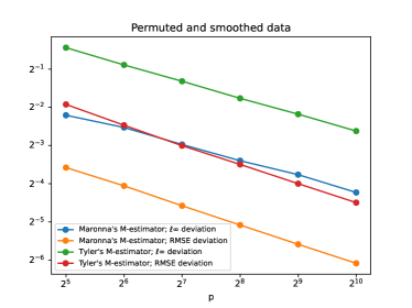
Fig. 1: The empirical deviation of the weights, plotted in log-log scale. Each point on the graph corresponds to the average of $50$ random repetitions.

Remark 4.

Observe that in Theorem 1, the weights of Maronna’s estimator do not depend on the population covariance $\Sigma_{p}$. This is because the weights are preserved under an arbitrary linear full-rank transformation of the data. Let ${\bf x}_{1},\ldots,{\bf x}_{n}$ and consider the transformed measurements $\tilde{{\bf x}}_{i}=A{\bf x}_{i}$, where $A\in\mathbb{R}^{p\times p}$ is full-rank. Denote the corresponding Marrona’s estimators (1) by $\hat{\Sigma}=\frac{1}{n}\sum_{i=1}^{n}w_{i}{\bf x}_{i}{\bf x}_{i}^{\top}$ and $\tilde{\Sigma}=\frac{1}{n}\sum_{i=1}^{n}\tilde{w}_{i}\tilde{{\bf x}}_{i}\tilde{{\bf x}}_{i}^{\top}$. One may verify that $\tilde{\Sigma}=A\hat{\Sigma}A^{\top}$, hence $w_{i}=\tilde{w}_{i}$; setting $A=\Sigma_{p}^{-1/2}$, we deduce that the weights $w^{\mbox{\tiny{Mar}}}_{i}$ do not depend on the covariance matrix of $X$.

In contrast, consistent with Theorem 2, the weights of Tyler’s estimator do depend on $\Sigma_{p}$. The reason is that while the linearly transformed estimator $A\hat{\Sigma}A^{\top}$ does solve the unconstrained Eq. (3), corresponding to the transformed measurements (similarly to Maronna’s estimator), one needs to rescale the weights due to the constraint ${\textrm{Tr}(\tilde{\Sigma})=p}$.

2.2 Regularized Estimators

We next consider the regularized variants of Maronna’s and Tyler’s M-estimators. As mentioned in Section 1, MRE exists uniquely for all $\gamma,\alpha>0$, whereas for any $\gamma>0$, TRE is only guaranteed to exist uniquely when $\alpha=\alpha(\gamma)>0$ is sufficiently large.

The regularization term $\frac{\alpha}{1+\alpha}\mathrm{I}_{p\times p}$ in Eqs. (2) and (4) shrinks the solution towards the identity matrix. As a result, the weights of MRE and TRE, and our deviation bounds for them, depend on the underlying population matrix $\Sigma_{p}$. Accordingly, throughout this section we operate under the following additional constraints on $\Sigma_{p}$, so to ensure that it has the same scale as the identity matrix. Specifically, for constants $s_{\max}\geq\tau>0$, we assume:

• Bounded operator norm:

  $$\|\Sigma_{p}\|\leq s_{\max}\,.$$ (10)

• Lower bound on total energy:

  $$\tau_{p}=\frac{1}{p}\textrm{Tr}\Sigma_{p}\geq\tau\,.$$ (11)

Towards stating our results, given a function $\phi(x)$, we define the following two functions ${Q,F:\mathbb{R}_{+}\to\mathbb{R}_{+}}$:

$$Q(d)=\frac{1}{p}{\mathbb{E}}\textrm{Tr}\Sigma_{p}\left(\phi(d)\sum_{i=1}^{n-1}{\bf x}_{i}{\bf x}_{i}^{\top}+\alpha d\mathrm{I}_{p\times p}\right)^{-1}\,,\quad F(d)=(1+\alpha)\frac{Q(d)}{1+\gamma\phi(d)Q(d)}\,.$$ (12)

As we shall see below, the functions $Q$ and $F$ play a decisive role in determining the weights of MRE and TRE. A key quantity is the solution $d^{*}>0$ to the following “master equation”:

$$F(d^{*})=1\,.$$ (13)

Later, we show that if $u(\cdot)$ is non-increasing and $\phi(x)=xu(x)$ is non-decreasing, then (13) admits a unique solution.

The theorem below regards Maronna’s regularized M-estimator. For $\varepsilon>0$, let $\mathcal{E}_{MRE}(\varepsilon)$ be the event that MRE exists uniquely with weights that satisfy

$$\max_{1\leq i\leq n}|w^{\mbox{\tiny{MRE}}}_{i}-u(d^{*})|\leq\varepsilon\,.$$ (14)

Theorem 3 (The weights of MRE.).

Let $\alpha>0$ and $u$ be a Lipschitz continuous on any compact sub-interval of $[0,\infty)$. Then, Eq. (13) has a unique solution which satisfies $d^{*}\in[\underline{d},\overline{d}]$, where the constants $0<\underline{d}\leq\overline{d}$ depend on the distribution of $Y$, $\gamma$, $\alpha$, $s_{\max}$ and $\tau$.

Furthermore, there are constants $c,C,\varepsilon_{0}>0$, that depend on the distribution of $Y$, $\gamma$, $\alpha$, $s_{\max}$ and $\tau$, such that for all $\varepsilon<\varepsilon_{0}$,

• Assume that $Y$ satisfies [LC]. Then $\Pr(\mathcal{E}_{MRE}(\varepsilon)^{c})\leq Cn^{2}e^{-c(\Psi_{p}\sqrt{n})\varepsilon}$.

• Assume that $Y$ satisfies either [SG-IND] or [CCP-SBP]. Then ${\Pr(\mathcal{E}_{MRE}(\varepsilon)^{c})\leq Cn^{2}e^{-cn\varepsilon^{2}}}$.

We note that the weights of MRE were previously studied in [6], assuming $Y$ has i.i.d. entries. They proved that asymptotically, as $n,p\to\infty$ at a fixed ratio $p/n=\gamma$, one has $\max_{1\leq i\leq n}\|w^{\mbox{\tiny{MRE}}}_{i}-u(d^{*})\|\to 0$ w.p. $1$.

Lastly, we consider Tyler’s regularized M-estimator (TRE). TRE is superficially a special case of MRE, corresponding to $u(x)=1/x$ and $\phi(x)=1$; a crucial difference, however, is that $u(\cdot)$ is singular at $x=0$. Accordingly, to carry out our analysis, we require an additional constraint on $\Sigma_{p}$: there exists a constant $\underline{\tau}>0$ such that

$$\frac{1}{p}\textrm{Tr}\Sigma_{p}^{-1}\leq\underline{\tau}\,.$$ (15)

For $\varepsilon>0$, let $\mathcal{E}_{TRE}(\varepsilon)$ be the event that TRE exists uniquely, and that furthermore its weights satisfy

$$\max_{1\leq i\leq n}|w^{\mbox{\tiny{TRE}}}_{i}-1/d^{*}|\leq\varepsilon\,.$$ (16)

Theorem 4 (The weights of TRE.).

Let $u(x)=1/x$, $\phi(x)=1$ and ${\alpha>\max\{0,\gamma-1\}}$. Then, Eq. (13) has a unique solution which satisfies $d^{*}\in[\underline{d},\overline{d}]$, where the constants $0<\underline{d}\leq\overline{d}$ depend on the distribution of $Y$, $\gamma$, $\alpha$, $s_{\max}$, $\tau$ and $\underline{\tau}$.

Furthermore, there are constant $c,C,\varepsilon_{0}>0$, that depend on the distribution of $Y$, $\gamma$, $\alpha$, $s_{\max}$, $\tau$ and $\underline{\tau}$, such that for all $\varepsilon<\varepsilon_{0}$,

• Assume that $Y$ satisfies [LC]. Then $\Pr(\mathcal{E}_{TRE}(\varepsilon)^{c})\leq Cn^{2}e^{-c(\Psi_{p}\sqrt{n})\varepsilon}$.

• Assume that $Y$ satisfies either [SG-IND] or [CCP-SBP]. Then ${\Pr(\mathcal{E}_{TRE}(\varepsilon)^{c})\leq Cn^{2}e^{-cn\varepsilon^{2}}}$.

For the special case where $X$ follows a Gaussian or an elliptical distribution, similar non-asymptotic concentration bounds for the weights of TRE were provided in [33]. Lastly, we remark that as noted in [33], the dependence on $\underline{\tau}$ can be removed when $\alpha$ is sufficiently large, i.e $\alpha\geq Cs_{\max}$ where $C$ is a suitable constant (see Remark 5 in D.3 for further details).

Paper outline

The rest of the manuscript is organized as follows. In Section 3 we provide definitions and technical background related to the distributional assumptions from Section 2 above. In Section 4 we describe some applications of our results to robust covariance and precision matrix estimation. Section 5 is devoted to the proofs of Theorems 1-4, with some technical details deferred to the Appendix. Finally, we offer some concluding remarks in Section 6.

3 Preliminaries and Technical Background

We provide a brief background and definitions for the distributions considered in Section 2. Recall that $Y\in\mathbb{R}^{p}$ is an isotropic random vector. Throughout this text, $\|\cdot\|$ denotes the Euclidean norm in the suitable dimension $p$.

Definition 1.

$Y$ is a sub-Gaussian vector with constant $K>0$ if for any $\|u\|=1$,

$$\Pr\left(\left|u^{\top}Y-{\mathbb{E}}[u^{\top}Y]\right|\geq t\right)\leq 2\exp\left[-(t/2K)^{2}\right]\,.$$

Sub-Gaussianity implies that linear functions of $Y$ concentrate. For our analysis we shall also need concentration of some sufficiently well-behaved non-linear functions. Following [3, 54], we consider the following property:

Definition 2.

$Y$ satisfies the convex concentration property (CCP) with constant $K>0$ if for every $1$-Lipschitz convex $f:\mathbb{R}^{p}\to\mathbb{R}$, the random variable $f(Y)$ is sub-Gaussian with constant $K$:

$$\Pr\left(\left|f(Y)-{\mathbb{E}}[f(Y)]\right|\geq t\right)\leq 2\exp\left[-(t/2K)^{2}\right]\,.$$ (17)

The CCP was introduced by Talagrand [73], who proved that if $Y$ has independent, uniformly bounded entries then it satisfies the CCP. Subsequent works established weaker conditions under which the CCP holds, see [2, 35] and references therein. Another family of distributions satisfying the CCP, which has received attention in machine learning and statistics (e.g. [13, 9, 64]), are the distributions satisfying a Log-Sobolev Inequality.

For parts of our analysis, we shall also need the following:

Definition 3.

$Y$ satisfies the small ball property (SBP) with constant $C_{0}$ if for any $\|u\|=1$ and $a\in\mathbb{R}$,

$$\Pr\left(\left|u^{\top}Y-a\right|\leq t\right)\leq C_{0}t\quad\textrm{ for all }t\geq 0\,.$$ (18)

The SBP is an anti-concentration property: it states that the law of $u^{\top}Y$ cannot put large mass around any particular value $a\in\mathbb{R}$. For our purposes, the SBP will be especially important for bounding the smallest eigenvalue of the sample covariance matrix, which is a key step in several of our proofs. Note that if the density of $u^{\top}Y$ is bounded, then (18) holds for some appropriate $C_{0}$. The following remarkable result, due to Rudelson and Vershynin, states that if $Y$ has independent entries, each with bounded density, then it satisfies the SBP [68, Theorem 1.2]:

Lemma 1.

Let $Y=(Y_{1},\ldots,Y_{p})$ have independent entries, with univariate densities all uniformly bounded by $C$. Then $Y$ satisfies the SBP with constant $2\sqrt{2}C$.

Log-concave distributions

We next consider the family of log-concave distributions on $\mathbb{R}^{p}$. This rich family has found multiple applications, for example, in statistics [7], pure mathematics [14, 71], computer science [10, 50] and economics [4]. Particular members in this family include the Gaussian, exponential, uniform over convex bodies, logistic, Gamma, Laplace, Weibull, Chi and Chi-Squared, Beta distributions and more.

Definition 4.

$Y$ is log-concave if it has a density $p_{Y}(y)=e^{-V(y)}$ for $V:\mathbb{R}^{p}\to\mathbb{R}\cup\{\infty\}$ convex.

It is known that log-concave random vectors are sub-exponential with a universal constant, see e.g. [14]. The following is implied by a recent breakthrough result of Klartag and Lehec [43, Theorem 1.1]:

Lemma 2.

There exists a universal $c>0$ and some $\Psi_{p}$ satisfying

$$(\log p)^{-5}\leq\Psi_{p}\leq 1$$ (19)

such that for every isotropic log-concave $Y\in\mathbb{R}^{p}$ and $1$-Lipschitz function $f(\cdot)$,

$$\Pr\left(\left|f(Y)-{\mathbb{E}}[f(Y)]\right|\geq t\right)\leq\exp\left[-c\Psi_{p}t\right]\,.$$ (20)

The quantity $\Psi_{p}$ is (up to a universal constant) the Cheeger constant corresponding to the family of log-concave distributions on $\mathbb{R}^{p}$. It is conjectured [39] that in fact $\Psi_{p}=\Theta(1)$ (the KLS conjecture). For background on the KLS conjecture and its consequences, see [46, 21]. Lastly, [50, Lemma 5.5] implies the following:

Lemma 3.

There is a universal $0<C_{0}\leq 2$ so that every isotropic log-concave $Y$ satisfies the SBP with constant $C_{0}$.

4 Applications to Robust Sparse Covariance and Inverse Covariance Estimation

As mentioned in the introduction, robust estimation of the covariance and inverse covariance matrices, given possibly heavy tailed data are important tasks in statistics. In high dimensional settings, these matrices are often assumed to be sparse, allowing their estimation from a limited number of samples. A common model for multivariate heavy tailed data, under which various estimators were derived and analyzed is to assume that the samples are elliptically distributed [41, 18, 32, 31]. Specifically, a random vector $\tilde{X}$ follows an elliptical distribution with mean $\bm{\mu}$ and shape matrix $\Sigma_{p}\in S^{p}_{++}$ if it has the form

$$\tilde{X}=\bm{\mu}+z\Sigma_{p}^{1/2}Y\,,$$ (21)

where $Y\sim\mathrm{Unif}(\mathbb{S}^{p-1})$, and $z$ is a strictly positive random variable which is independent of $Y$ (but otherwise arbitrary). To make the model (21) identifiable, the scaling $p^{-1}\textrm{Tr}\Sigma_{p}=1$ is assumed.

The authors of [33] considered the problem of shape matrix estimation under a sparsity constraint. They showed that given (possibly heavy tailed) elliptical samples, a sparse $\Sigma_{p}$ may nonetheless be estimated at the same rate as if one had sub-Gaussian samples with covariance $\Sigma_{p}$. Their estimator is remarkably simple: compute Tyler’s M-estimator corresponding to the $n$ samples, and then threshold its entries as proposed by [12].

In this section, building upon the theorems of Section 2, we show that the above approach yields accurate estimates for heavy tailed distributions beyond the elliptical model (21). Specifically, the vector $Y$ in (21) may be replaced by any isotropic random vector satisfying the assumptions of Section 2. Furthermore, we show a similar result for estimating the inverse shape matrix $\Sigma_{p}^{-1}$ assuming it is sparse. For simplicity, we assume that $\tilde{X}$ is zero mean with $\bm{\mu}=\bm{0}$ whereas in Section 6 we discuss how this restriction may be overcome.

4.1 Sparse shape matrix estimation

Observe that Tyler’s M-estimator, Eq. (3), is invariant to an arbitrary scaling of the samples. Consequently, Tyler’s estimator computed from the elliptically-distributed samples $\tilde{{\bf x}}_{i}=z_{i}\Sigma_{p}^{1/2}{\bf y}_{i}$, call it $\hat{\Sigma}_{\mbox{\tiny{Tyl}}}$, is exactly the same as the estimator computed from the rescaled samples ${\bf x}_{i}=\Sigma_{p}^{1/2}{\bf y}_{i}$. We emphasize that the rescaled vectors ${\bf x}_{1},\ldots,{\bf x}_{n}$ are not available to the estimator. Denote $S=n^{-1}\sum_{i=1}^{n}{\bf x}_{i}{\bf x}_{i}^{\top}$, and $\hat{\Sigma}_{\mbox{\tiny{Tyl}}}=n^{-1}\sum_{i=1}^{n}w^{\mbox{\tiny{Tyl}}}_{i}{\bf x}_{i}{\bf x}_{i}^{\top}$. For a matrix $M$, denote the norms,

$$\|M\|_{\max}=\max_{i,j}|M_{ij}|,\quad\|M\|_{1}=\sum_{i,j}|M_{ij}|\,.$$

We start with the following important lemma, which asserts that $\hat{\Sigma}_{\mbox{\tiny{Tyl}}}$ is close to $\Sigma_{p}$ entrywise:

Lemma 4.

Assume the setting of Theorem 2, recalling the normalization $\tau_{p}=1$. There is $C>0$, that depends on the distribution of $Y$ and on $\gamma$, such that w.p. $1-o(1)$, the following holds.

1. Assume that $Y$ satisfies [LC]. Then $\|\hat{\Sigma}_{\mbox{\tiny{Tyl}}}-\Sigma_{p}\|_{\max}\leq C\|\Sigma_{p}\|\frac{\log p}{\Psi_{p}\sqrt{n}}$.

2. Assume that $Y$ satisfies either [SG-IND] or [CCP-SBP]. Then $\|\hat{\Sigma}_{\mbox{\tiny{Tyl}}}-\Sigma_{p}\|_{\max}\leq C\|\Sigma_{p}\|\sqrt{\frac{\log p}{n}}$.

Proof.

By the triangle inequality, $\|\hat{\Sigma}_{\mbox{\tiny{Tyl}}}-\Sigma_{p}\|_{\max}\leq\|\hat{\Sigma}_{\mbox{\tiny{Tyl}}}-S\|_{\max}+\|S-\Sigma_{p}\|_{\max}$. We bound the second term, by Lemma 23 in the Appendix, which bounds the deviations of the entries of $S$ about their expectation $\Sigma_{p}$. For the first term,

$${\|\hat{\Sigma}_{\mbox{\tiny{Tyl}}}-S\|_{\max}\leq}\|\hat{\Sigma}_{\mbox{\tiny{Tyl}}}-S\|=\left\|\frac{1}{n}\sum_{i=1}^{n}(w^{\mbox{\tiny{Tyl}}}_{i}-1){\bf x}_{i}{\bf x}_{i}^{\top}\right\|\leq\max_{1\leq i\leq n}|w^{\mbox{\tiny{Tyl}}}_{i}-1|\cdot\|S\|\,.$$

By Lemma 20 in the Appendix, $\|S\|\lesssim\|\Sigma_{p}\|$ w.h.p., whereas $\max_{1\leq i\leq n}|w^{\mbox{\tiny{Tyl}}}_{i}-1|$ may be bounded by Theorem 2. ∎

Following Bickel and Levina [12], consider the class of approximately sparse covariance matrices, $q\in[0,1)$,

$$\mathcal{U}_{p}(q,s_{q}(p))=\left\{\Sigma\in\mathcal{S}_{++}^{p}\;:\;\,\sum_{j=1}^{p}|\Sigma_{ij}|^{q}\leq s_{q}(p),\,1\leq i\leq p\right\}\,.$$ (22)

Let $\mathcal{T}_{t}$ be the entry-wise hard-thresholding operator $\mathcal{T}_{t}(M)_{ij}=M_{ij}\mathbbm{1}_{\left\{|M_{ij}|\geq t\right\}}$. The authors of [12] showed that to accurately estimate a matrix $\Sigma_{p}\in\mathcal{U}_{p}(q,s_{q}(p))$ with respect to operator norm, it suffices to construct a matrix $A$ which is close to $\Sigma_{p}$ entrywise, and then threshold it. We cite the following form of their result, as stated in [33, Lemma 6]:

Lemma 5.

Let $\Sigma_{p}\in\mathcal{U}_{p}(q,s_{q}(p))$ and $A$ such that $\|A-\Sigma_{p}\|_{\max}\leq\varepsilon$. There is a threshold $t=c_{1}\varepsilon$ so that for some $c_{2}=c_{2}(q)$, $\|\mathcal{T}_{t}(A)-\Sigma_{p}\|\leq c_{2}s_{q}(p)\varepsilon^{1-q}$.

Combining Lemmas 4 and 5 yields the following generalization of [33, Theorem 1], which proved a similar result under the more restrictive assumption that $Y$ has an elliptical distribution:

Corollary 1.

There are $c,C>0$, that may depend on the distribution of $Y$ and on $\gamma$, such that the following holds. For an appropriately chosen threshold $t$, if $\Sigma_{p}\in\mathcal{U}_{p}(q,s_{q}(p))$, then w.p. $1-o(1)$,

1. Assume that $Y$ satisfies [LC]. Then $\|\Sigma_{p}-\mathcal{T}_{t}(\hat{\Sigma}_{\mbox{\tiny{Tyl}}})\|\leq Cs_{q}(p)\|\Sigma_{p}\|^{1-q}\left(\frac{(\log p)^{2}}{\Psi_{p}^{2}n}\right)^{(1-q)/2}$.

2. Assume that $Y$ satisfies either [SG-IND] or [CCP-SBP]. Then $\|\Sigma_{p}-\mathcal{T}_{t}(\hat{\Sigma}_{\mbox{\tiny{Tyl}}})\|\leq Cs_{q}(p)\|\Sigma_{p}\|^{1-q}\left({\frac{\log p}{n}}\right)^{(1-q)/2}$.

Under [SG-IND] and [CCP-SBP], the attained rate is minimax optimal in $n,p$ [17].

4.2 Sparse inverse shape matrix estimation

We now consider the problem of estimating $\Sigma_{p}^{-1}$, assuming that it is sparse: $\Sigma_{p}^{-1}\in\mathcal{U}_{p}(q,s_{q}(p))$. Cai et. al. proposed the CLIME estimator [15], which solves a linear program of the form:

$$\min_{\Omega}\|\Omega\|_{1}\quad\textrm{subject to}\quad\|\hat{S}\Omega-\mathrm{I}_{p\times p}\|_{\max}\leq\lambda\,,$$ (23)

where $\lambda$ is a tuning parameter and $\hat{S}$ is a proxy for $\Sigma_{p}$ ([15] propose to use the data sample covariance matrix). Having solved (23), a symmetrization step is applied to get the final estimator. [15, Theorem 6] states that if $\hat{S}$ is close entrywise to $\Sigma_{p}$, then the estimator $\hat{\Omega}=\hat{\Omega}(\hat{S})$ is close in operator norm to $\Sigma_{p}^{-1}$:

Lemma 6.

Suppose that $\Sigma_{p}^{-1}\in\mathcal{U}_{p}(q,s_{q}(p))$ and $\hat{S}$ satisfies $\|\Sigma_{p}-\hat{S}\|_{\max}\leq\varepsilon$. For any $\lambda\geq\|\Sigma_{p}^{-1}\|_{1}\varepsilon$, the estimator obtained by solving (23) and applying symmetrization satisfies $\|\hat{\Omega}-\Sigma_{p}^{-1}\|\leq Cs_{q}(p)\|\Sigma_{p}^{-1}\|_{1}^{1-q}\lambda^{1-q}$.

Setting $\hat{S}=\hat{\Sigma}_{\mbox{\tiny{Tyl}}}$ in (23) and using Lemma 4, yields:

Corollary 2.

There are $c,C>0$, that may depend on the distribution of $Y$ and on $\gamma$, such that the following holds. For an appropriately chosen $\lambda$, if $\Sigma_{p}^{-1}\in\mathcal{U}_{p}(q,s_{q}(p))$, then w.p. $1-o(1)$,

1. Assume that $Y$ satisfies [LC]. Then $\|\Sigma_{p}^{-1}-\hat{\Omega}(\hat{\Sigma}_{\mbox{\tiny{Tyl}}})\|\leq Cs_{q}(p)\|\Sigma_{p}^{-1}\|_{1}^{2-q}\|\Sigma_{p}\|^{1-q}\left(\frac{(\log p)^{2}}{\Psi_{p}^{2}n}\right)^{(1-q)/2}$.

2. Assume that $Y$ satisfies either [SG-IND] or [CCP-SBP]. Then $\|\Sigma_{p}^{-1}-\hat{\Omega}(\hat{\Sigma}_{\mbox{\tiny{Tyl}}})\|\leq Cs_{q}(p)\|\Sigma_{p}^{-1}\|_{1}^{2-q}\|\Sigma_{p}\|^{1-q}\left({\frac{\log p}{n}}\right)^{(1-q)/2}$.

Lastly, we remark that CLIME is known to have a sub-optimal rate for i.i.d. sub-Gaussian data. In [16], the minimax rate is computed and a rate-optimal adaptive estimator ACLIME is proposed. While beyond the scope of the present paper, we conjecture that a similar result, as Corollary 2, may be derived for ACLIME as well.

5 Proofs

Recall that the input data consists of $n$ samples ${\bf x}_{i}=\Sigma_{p}^{1/2}{\bf y}_{i}$ with ${\bf y}_{i}$ isotropic. Denote by $S$ (resp. $T$) the sample covariance corresponding to the ${\bf x}_{i}$-s (resp. ${\bf y}_{i}$-s),

$$S=\frac{1}{n}\sum_{i=1}^{n}{\bf x}_{i}{\bf x}_{i}^{\top}=\Sigma_{p}^{1/2}T\Sigma_{p}^{1/2}\,,\quad T=\frac{1}{n}\sum_{i=1}^{n}{\bf y}_{i}{\bf y}_{i}^{\top}.$$

For $1\leq j\leq n$, denote by $S_{-j}$ (similarly $T_{-j}$) the sample covariance of $(n-1)$ samples excluding ${\bf x}_{j}$,

$$S_{-j}=S-\frac{1}{n}{\bf x}_{i}{\bf x}_{i}^{\top}=\frac{1}{n}\sum_{i=1,i\neq j}^{n}{\bf x}_{i}{\bf x}_{i}^{\top}\,.$$

The following lemma, proven in B, is key to the analysis of Maronna’s and Tyler’s estimators.

Lemma 7.

Assume $\gamma<1$. There are $c,C,\varepsilon_{0}>0$, that depend on the distribution of $Y$ and on $\gamma$, so that for all $\varepsilon<\varepsilon_{0}$:

1. Assume [LC]. Then $\Pr(\max_{1\leq i\leq n}|p^{-1}{\bf x}_{i}^{\top}S^{-1}{\bf x}_{i}-1|\geq\varepsilon)\leq Cn^{2}e^{-c(\Psi_{p}\sqrt{n})\varepsilon}$.

2. Assume [SG-IND]  or [CCP-SBP]. Then $\Pr(\max_{1\leq i\leq n}|p^{-1}{\bf x}_{i}^{\top}S^{-1}{\bf x}_{i}-1|\geq\varepsilon)\leq Cn^{2}e^{-cn\varepsilon^{2}}$.

Note that ${\bf x}_{i}^{\top}S^{-1}{\bf x}_{i}={\bf y}_{i}^{\top}\Sigma_{p}^{1/2}(\Sigma_{p}^{1/2}T\Sigma_{p}^{1/2})^{-1}\Sigma_{p}^{1/2}{\bf y}_{i}={\bf y}_{i}^{\top}T^{-1}{\bf y}_{i}$, so the quadratic form $p^{-1}{\bf x}_{i}^{\top}S^{-1}{\bf x}_{i}$ does not depend on $\Sigma_{p}$. Assuming that ${\bf x}_{i}$-s are Gaussian, a similar result was derived in [79]. Their proof relies on the orthogonal invariance of the isotropic Gaussian distribution, and does not generalize to other distributions. Lemma 7 implies that $\max_{1\leq i\leq n}|{\bf x}_{i}^{\top}S^{-1}{\bf x}_{i}-1|\to 1$ w.p. $1$ in the asymptotic limit $n,p\to\infty$ with $\frac{p}{n}\to\gamma$. Assuming $Y$ has independent entries with finite fourth moment, this asymptotic result was proven in [25].

5.1 Proof of Theorem 1 (Maronna’s M-Estimator)

Existence

We first prove that a solution to the fixed point equation (1) indeed exists. This proof follows that of [25]. We briefly describe it, for the sake of completeness. Denote $\mathbf{d}=(d_{1},\ldots,d_{n})$. Consider the function $h:\mathbb{R}_{+}^{n}\to\mathbb{R}_{+}^{n}$,

$$h_{j}(\mathbf{d})=\frac{1}{p}{\bf x}_{j}^{\top}\left(\frac{1}{n}\sum_{i=1}^{n}u(d_{i}){\bf x}_{i}{\bf x}_{i}^{\top}\right)^{-1}{\bf x}_{j},\quad 1\leq j\leq n\,.$$ (24)

Since by assumption $X$ has a density and $n>p$, $h$ is well-defined w.p. 1. Moreover, a vector $\bm{d}$ yields a Maronna’s estimator with weights $w_{j}=u(d_{j})$ if and only if $d_{j}=h_{j}(\mathbf{d})$ for all $j$. Hence, to establish the existence of Maronna’s estimator, we need to show that $h$ has a fixed point. To this end, as proven in [25], the function $h(\cdot)$ satisfies the following three properties. 1) Positivity: $h(\mathbf{d})>\mathbf{0}$ for any vector $\mathbf{d}\geq\mathbf{0}$, namely with $d_{j}\geq 0$ for all $j$; 2) Monotonicity: if $\mathbf{d}\geq\mathbf{d}^{\prime}\geq\mathbf{0}$, then $h(\mathbf{d})\geq h(\mathbf{d}^{\prime})$; 3) Scalability: for any $\alpha>1$, $\alpha h(\mathbf{d})\geq h(\alpha\mathbf{d})$. A function $h(\cdot)$ satisfying these properties is (almost) a standard interference function, in the sense of [78]. By [78, Theorem 1], if there exists some $\mathbf{d}$ with $\mathbf{d}\geq h(\mathbf{d})$, then $h(\cdot)$ has a fixed point. The following lemma shows that w.h.p., such a vector ${\bf d}$ exists, which in turn implies the existence of Maronna’s estimator.

Lemma 8.

There are $c,C>0$, that depend on the distribution of $Y$ and on $\gamma$, such that

1. Assume [LC]. $\Pr\left(\exists\bm{d}>\bm{0}\;:\;\bm{d}\geq h(\bm{d})\right)\geq 1-Cn^{2}e^{-c(\Psi_{p}\sqrt{n})}$.

2. Assume [SG-IND]  or [CCP-SBP]. Then $\Pr\left(\exists\bm{d}>\bm{0}\;:\;\bm{d}\geq h(\bm{d})\right)\geq 1-Cn^{2}e^{-cn}$.

Proof.

By assumption (i) of Theorem 1, $\phi_{\infty}>1$. Hence, we may take some $d_{0}>0$ such that $\phi(d_{0})>1$. Setting $\bm{d}_{0}=d_{0}\bm{1}=(d_{0},\ldots,d_{0})$ in (24) and using $u(d)=\phi(d)/d$, one may verify that $h_{j}(\bm{d}_{0})=\frac{d_{0}}{\phi(d_{0})}\frac{1}{p}{\bf x}_{j}^{\top}S^{-1}{\bf x}_{j}$. By Lemma 7, w.h.p., $\max_{1\leq j\leq n}\frac{1}{p}{\bf x}_{j}^{\top}S^{-1}{\bf x}_{j}\leq\phi(d_{0})$, and so $h(\bm{d}_{0})\leq\bm{d}_{0}$. ∎

Uniqueness and concentration

Let $\mathbf{d}=(d_{1},\ldots,d_{n})$ be a vector satisfying $h(\mathbf{d})=\mathbf{d}$, which yields a valid Maronna’s estimator. Next, we prove that only one such $\bm{d}$ exists. To this end, denote $j_{\min}=\operatorname*{\arg\!\min}_{1\leq j\leq n}d_{j}$, $j_{\max}=\operatorname*{\arg\!\max}_{1\leq j\leq n}d_{j}$. Since $h(\cdot)$ is non-decreasing, $d_{j}=h_{j}(\bm{d})\leq h_{j}(d_{j_{\max}}\bm{1})=(u(d_{j_{\max}}))^{-1}p^{-1}{\bf x}_{j}^{\top}S^{-1}{\bf x}_{j}$. Setting $j=j_{\max}$ and multiplying by $u(d_{j_{\max}})$ gives $\phi(d_{j_{\max}})\leq p^{-1}{\bf x}_{j_{\max}}^{\top}S^{-1}{\bf x}_{j_{\max}}$. Similarly, $h(\bm{d})\geq h(d_{j_{\min}}\bm{1})$, and thus $\phi(d_{j_{\min}})\geq p^{-1}{\bf x}_{j_{\min}}^{\top}S^{-1}{\bf x}_{j_{\min}}$. Finally, since $\phi$ is non-decreasing, we deduce that for all $j$, $p^{-1}{\bf x}_{j_{\min}}^{\top}S^{-1}{\bf x}_{j_{\min}}\leq\phi(d_{j})\leq p^{-1}{\bf x}_{j_{\max}}^{\top}S^{-1}{\bf x}_{j_{\max}}$. Consequently,

$$\max_{1\leq j\leq n}|\phi(d_{j})-1|\leq\max_{1\leq j\leq n}|p^{-1}{\bf x}_{j}^{\top}S^{-1}{\bf x}_{j}-1|\,.$$ (25)

The next lemma shows that w.h.p., $h(\cdot)$ cannot have any fixed points whose entries are far from the constant $\phi^{-1}(1)$:

Lemma 9.

For $\varepsilon>0$, let $\mathcal{F}_{\mathrm{bad}}(\varepsilon)$ the set of “bad” fixed points of $h(\cdot)$, namely, such that ${\|\bm{d}-\phi^{-1}(1)\bm{1}\|_{\infty}\geq\varepsilon}$. There $c,C,\varepsilon_{0}>0$, that depend on the distribution of $Y$ and on $\gamma$, such that for all $\varepsilon<\varepsilon_{0}$,

1. Assume [LC]. Then $\Pr\left(\mathcal{F}_{\mathrm{bad}}(\varepsilon)\neq\emptyset\right)\leq Cn^{2}e^{-c(\Psi_{p}\sqrt{n})\varepsilon}.$

2. Assume [SG-IND]  or [CCP-SBP]. Then $\Pr\left(\mathcal{F}_{\mathrm{bad}}(\varepsilon)\neq\emptyset\right)\leq Cn^{2}e^{-cn\varepsilon^{2}}.$

Proof.

Follows immediately by Lemma 7, Eq. (25) and Assumption (ii) of Theorem 1, which states that $\phi$ is invertible in a neighborhood of $\phi^{-1}(1)$ and that the inverse $\phi^{-1}$ is locally Lipshitz at $1$. ∎

Lastly, we prove that Maronna’s estimator exists uniquely w.h.p:

Lemma 10.

There are $c,C>0$, that depend on the distribution of $Y$ and on $\gamma$, such that

1. Assume [LC]. Then $\Pr\left(\textrm{ME exists uniquely}\right)\geq 1-Cn^{2}e^{-c(\Psi_{p}\sqrt{n})}$.

2. Assume [SG-IND]  or [CCP-SBP]. Then $\Pr\left(\textrm{ME exists uniquely}\right)\geq 1-Cn^{2}e^{-cn}$.

Proof.

Existence, w.h.p., is guaranteed by Lemma 8. Assume by contradiction that $h$ has two different fixed points, $\mathbf{d}\neq\mathbf{d}^{\prime}$. Take $\alpha=\max_{j}(d_{j}/d_{j}^{\prime})$, and let $l$ be a coordinate where the maximum is attained. Assume w.l.o.g. that $\alpha>1$ (otherwise replace $\mathbf{d}$ with $\mathbf{d}^{\prime}$), and note that by its definition, $\mathbf{d}\leq\alpha\mathbf{d}^{\prime}$.

Let $\eta>0$ be so that $\phi(\cdot)$ is strictly increasing in $[\phi^{-1}(1)-\eta,\phi^{-1}(1)+\eta]$. By Lemma 9, w.h.p. both $\mathbf{d},\mathbf{d}^{\prime}\in[\phi^{-1}(1)-\eta/2,\phi^{-1}(1)+\eta/2]^{n}$. In addition, since $\alpha>1$, then $\phi(\alpha d_{j}^{\prime})>\phi(d_{j}^{\prime})$ for all $j$. This, in turn, implies that

$$u(\alpha d_{j}^{\prime})=\frac{\phi(\alpha d_{j}^{\prime})}{\alpha d_{j}^{\prime}}>\frac{\phi(d_{j}^{\prime})}{\alpha d_{j}^{\prime}}=\frac{1}{\alpha}u(d_{j}^{\prime})\,.$$

Plugging this into (24) gives $h(\alpha\bm{d}^{\prime})<\alpha h(\bm{d}^{\prime})$. Since $\mathbf{d}\leq\alpha\mathbf{d}^{\prime}$ and $h$ is non-decreasing, we deduce $h(\bm{d})<\alpha h(\bm{d}^{\prime})$. But, since $\mathbf{d},\mathbf{d}^{\prime}$ are fixed points of $h(\cdot)$, this yields a contradiction: $d_{l}=h_{l}({\bf d})<\alpha h_{l}(\mathbf{d}^{\prime})=\alpha d_{l}^{\prime}=d_{l}\,.$ ∎

Proof of Theorem 1

Existence and uniqueness follow from Lemma 10. By Lemma 9, the coordinates of the fixed point ${\bf d}$ concentrate around $\phi^{-1}(1)$. Hence, the weights of Maronna’s estimator, $w^{\mbox{\tiny{Mar}}}_{i}=u(d_{i})$, concentrate around $u(\phi^{-1}(1))=\phi(\phi^{-1}(1))/\phi^{-1}(1)=1/\phi^{-1}(1)$. ∎

5.2 Proof of Theorem 2 (Tyler’s M-Estimator)

Our proof combines the strategy of Zhang et. al. [79] with Lemma 7. Since $X$ has a density, by [42, Theorems 1 and 2] Tyler’s estimator exists uniquely w.p. $1$. By [79, Lemma 2.1], its weights are

$$w^{\mbox{\tiny{Tyl}}}_{i}=\frac{p\cdot\widehat{w}_{i}}{\textrm{Tr}\left(\frac{1}{n}\sum_{i=1}^{n}\widehat{w}_{i}{\bf x}_{i}{\bf x}_{i}^{\top}\right)}\,,$$ (26)

where $\widehat{{\bf w}}=(\widehat{w}_{1},\ldots,\widehat{w}_{n})$ is the unique minimizer of

$$F({\bf w})=-\sum_{i=1}^{n}\log w_{i}+\frac{n}{p}\log\det\left(\sum_{i=1}^{n}w_{i}{\bf x}_{i}{\bf x}_{i}^{\top}\right),\quad\textrm{subject to }{\bf w}>\bm{0}\textrm{ and }\sum_{i=1}^{n}{\bf w}_{i}=n\,.$$ (27)

As in [79], the proof proceeds in two steps: (I) Show that $\widehat{w}_{1},\ldots,\widehat{w}_{n}$ all concentrate around $1$; (II) Using (26), deduce concentration for the weights $w^{\mbox{\tiny{Tyl}}}_{1},\ldots,w^{\mbox{\tiny{Tyl}}}_{n}$.

We start with the weights $\widehat{{\bf w}}$. The argument of [79, Section 3.2] starts with the following observation:

Lemma 11.

Let $\beta>0$ be arbitrary. Then $\widehat{{\bf w}}$ is the unique stationary point of the following function $G_{\beta}:\mathbb{R}^{n}\to\mathbb{R}$:

$$G_{\beta}({\bf w})=F({\bf w})+\frac{\beta}{2}\left(\sum_{i=1}^{n}w_{i}-n\right)^{2}=-\sum_{i=1}^{n}\log w_{i}+\frac{n}{p}\log\det\left(\sum_{i=1}^{n}w_{i}{\bf x}_{i}{\bf x}_{i}^{\top}\right)+\frac{\beta}{2}\left(\sum_{i=1}^{n}w_{i}-n\right)^{2}\,.$$ (28)

Next, note that ${\bf w}={\bf 1}=(1,\ldots,1)$ is “almost” a zero of $g_{\beta}(\cdot)=\nabla G_{\beta}(\cdot)$ (for any $\beta$), in the sense that w.h.p. $g_{\beta}({\bf 1})$ is small. Indeed, a straightforward calculation, Appendix Eq. (47), gives

$$\left(g_{\beta}({\bf 1})\right)_{\ell}=-1+\frac{1}{p}{\bf x}_{\ell}^{\top}\left(\frac{1}{n}\sum_{i=1}^{n}{\bf x}_{i}{\bf x}_{i}^{\top}\right)^{-1}{\bf x}_{\ell}=-1+\frac{1}{p}{\bf x}_{\ell}^{\top}S^{-1}{\bf x}_{\ell}\,\quad\textrm{for all }1\leq\ell\leq n\,.$$ (29)

By Lemma 7, the right-hand-side of (29) concentrates tightly around $0$. That is, the following deviation bound holds:

Lemma 12.

There are $c,C,\varepsilon_{0}>0$, that depend on the distribution of $Y$ and on $\gamma$, so that for all $\varepsilon<\varepsilon_{0}$ and all $\beta$

1. Assume [LC]. Then $\Pr\left(\|g_{\beta}({\bf 1})\|_{\infty}\geq\varepsilon\right)\leq Cn^{2}e^{-c(\Psi_{p}\sqrt{n})\varepsilon}$.

2. Assume either [SG-IND]  or [CCP-SBP]. Then $\Pr\left(\|g_{\beta}({\bf 1})\|_{\infty}\geq\varepsilon\right)\leq Cn^{2}e^{-cn\varepsilon^{2}}$.

Next, we carry out a perturbation argument: we show that $\|g_{\beta}(\bm{1})\|_{\infty}$ being small implies that the unique root $g_{\beta}(\widehat{{\bf w}})=\bm{0}$ is close to $\bm{1}$. To this end, we use the following result, [79, Lemma 3.1]. Below, for a matrix $M\in\mathbb{R}^{n\times n}$, we denote by $\|M\|_{\infty,\infty}=\max_{1\leq j\leq n}\sum_{\ell=1}^{n}|M_{j\ell}|$ its $\ell_{\infty}$-to-$\ell_{\infty}$ operator norm.

Lemma 13.

Let $h:\mathbb{R}^{p}\to\mathbb{R}^{p}$ be differentiable, ${\bf w}_{0}\in\mathbb{R}^{p}$. Suppose that for some $L,R>0$ and $0<\varepsilon\leq\min\{R,L^{-1}\}$:

1. (${\bf w}_{0}$ is “almost” a zero). $\|h({\bf w}_{0})\|_{\infty}\leq\frac{1}{2}\varepsilon$.

2. (Non-degeneracy at ${\bf w}_{0}$). $\nabla h({\bf w}_{0})=\mathrm{I}_{p\times p}$, namely $\left(\nabla h\right)_{j,\ell}=\frac{\partial h_{j}}{\partial w_{\ell}}=\delta_{j,\ell}$.

3. (Smoothness around ${\bf w}_{0}$). $\|\nabla h({\bf w})-\nabla h({\bf w}_{0})\|_{\infty,\infty}\leq L\|{\bf w}-{\bf w}_{0}\|_{\infty}$ for all ${\bf w}$ in ${\|{\bf w}-{\bf w}_{0}\|_{\infty}\leq R}$.

Then $h(\cdot)$ has a zero $\widehat{{\bf w}}$ close to ${\bf w}_{0}$ such that $\|\widehat{{\bf w}}-{\bf w}_{0}\|_{\infty}\leq\varepsilon$.

To prove that $g_{\beta}$ has a zero near ${\bf w}_{0}=\bm{1}$ via Lemma 13, we consider $h_{\beta}({\bf w})=\left(\nabla g_{\beta}({\bf 1})\right)^{-1}g_{\beta}({\bf w})$. Clearly, $g_{\beta}$ and $h_{\beta}$ have the same zeros. Also, by its definition, $h_{\beta}$ satisfies condition (II) above. We next show that w.h.p. $h_{\beta}$ satisfies condition (I). Since $\|h_{\beta}(\bm{1})\|_{\infty}\leq\left\|\left(\nabla g_{\beta}({\bf 1})\right)^{-1}\right\|_{\infty,\infty}\|g_{\beta}({\bf 1})\|_{\infty}$, it suffices to bound the matrix norm $\left\|\left(\nabla g_{\beta}({\bf 1})\right)^{-1}\right\|_{\infty,\infty}$:

Lemma 14.

There are $c,C,B,\beta_{0}>0$, that depend the distribution of $Y$ and on $\gamma$, so that setting $\beta=\beta_{0}/n$,

1. Assume  [LC]. Then $\Pr\left(\|\left(\nabla g_{\beta}({\bf 1})\right)^{-1}\|_{\infty,\infty}\geq B\right)\leq Cn^{2}e^{-c\Psi_{p}n^{1/4}}$.

2. Assume [SG-IND] or [CCP-SBP]. Then $\Pr\left(\|\left(\nabla g_{\beta}({\bf 1})\right)^{-1}\|_{\infty,\infty}\geq B\right)\leq Cn^{2}e^{-cn^{1/2}}$.

We prove Lemma 14 in C.1. Our proof follows Zhang et. al. [79, Lemma 3.3]. Their argument, however, contains a mathematical error that we correct.

Lastly, we address condition (III) of Lemma 13. We prove the following in C.2:

Lemma 15.

Let $L_{g}$ be the $\ell_{\infty}$ Lipschitz constant of $\nabla g_{\beta}$ on an $\ell_{\infty}$ ball of radius $\frac{1}{2}$ around ${\bf 1}$:

$$L_{g}=\max_{{\bf w}\,:\,\|{\bf w}-{\bf 1}\|_{\infty}\leq\frac{1}{2}}\frac{\|\nabla g_{\beta}({\bf w})-\nabla g_{\beta}({\bf 1})\|_{\infty,\infty}}{\|{\bf w}-{\bf 1}\|_{\infty}}\,.$$

There are $c,C,L>0$, that depend on the distribution of $Y$ and on $\gamma$, so that

1. Assume [LC]. Then $\Pr(L_{g}\geq L)\leq Cn^{2}e^{-c\Psi_{p}\sqrt{n}}$.

2. Assume [SG-IND]  or [CCP-SBP]. Then $\Pr(L_{g}\geq L)\leq Cn^{2}e^{-cn}$.

Equipped with the preceding lemmas, we are ready to prove our concentration result for $\widehat{{\bf w}}$:

Lemma 16.

Let $\widehat{{\bf w}}=(\widehat{w}_{1},\ldots,\widehat{w}_{n})>\bm{0}$ be the unique minimizer of (27). There are $c,C,\varepsilon_{0}>0$, that depend on the distribution of $Y$ and on $\gamma$, such that for all $\varepsilon<\varepsilon_{0}$,

1. Assume [LC]. Then $\Pr\left(\max_{1\leq i\leq n}\left|\widehat{w}_{i}-1\right|\geq\varepsilon\right)\leq Cn^{2}e^{-c\Psi_{p}\min\left\{\sqrt{n}\varepsilon,\,n^{1/4}\right\}}$.

2. Assume [SG-IND] or [CCP-SBP]. Then $\Pr\left(\max_{1\leq i\leq n}\left|\widehat{w}_{i}-1\right|\geq\varepsilon\right)\leq Cn^{2}e^{-c\min\left\{n\varepsilon^{2},\,n^{1/2}\right\}}$.

Proof.

Choose $\beta=\beta_{0}/n$ per Lemma 14, such that $\|\left(\nabla g_{\beta}({\bf 1})\right)^{-1}\|_{\infty,\infty}\leq B$ holds w.h.p. By Lemma 15, for some $L>0$, w.h.p. $\|\nabla g_{\beta}({\bf w})-\nabla g_{\beta}({\bf 1})\|_{\infty,\infty}\leq\frac{L}{B}\|{\bf w}-{\bf 1}\|_{\infty}$ holds uniformly inside the $\ell_{\infty}$ ball $\|{\bf w}-{\bf 1}\|_{\infty}\leq\frac{1}{2}$. By Lemma 12, $\|g_{\beta}({\bf 1})\|_{\infty}<\frac{\varepsilon}{2B}$ holds w.h.p. Under the intersection of these events, $h_{\beta}({\bf w})=\left(\nabla g_{\beta}({\bf 1})\right)^{-1}g_{\beta}({\bf w})$ satisfies the conditions of Lemma 13, with constants $R=\frac{1}{2}$ and $L$. Assuming $\varepsilon\leq\varepsilon_{0}:=\min\{\frac{1}{2},L^{-1}\}$, by Lemma 13 $h_{\beta}(\cdot)$ has a zero ${\bf w}^{*}$, equivalently a stationary point of $G_{\beta}(\cdot)$, with $\|{\bf w}^{*}-{\bf 1}\|_{\infty}\leq\varepsilon$. By Lemma 11, ${\bf w}^{*}=\widehat{{\bf w}}$.

∎

Of Theorem 2.

Recall that the weights $w^{\mbox{\tiny{Tyl}}}_{i}$ are related to $\widehat{w}_{i}$ via (26). Denote $\tau_{p}=p^{-1}\textrm{Tr}(\Sigma_{p})$. Under the high-probability event $\max_{1\leq i\leq n}|\widehat{w}_{i}-1|\leq\varepsilon$, we have

$$\frac{1-\varepsilon}{(1+\varepsilon)\cdot p^{-1}\textrm{Tr}(S)/\tau_{p})}\leq\tau_{p}w^{\mbox{\tiny{Tyl}}}_{i}=\frac{\widehat{w}_{i}}{\tau_{p}^{-1}p^{-1}\textrm{Tr}\left(\frac{1}{n}\sum_{i=1}^{n}\widehat{w}_{i}{\bf x}_{i}{\bf x}_{i}^{\top}\right)}\leq\frac{1+\varepsilon}{(1-\varepsilon)\cdot p^{-1}\textrm{Tr}(S)/\tau_{p}}\,.$$ (30)

We next show that the denominator of (30) concentrates tightly around $1$, namely, that w.h.p. $|p^{-1}\textrm{Tr}(S)-\tau_{p}|\leq\varepsilon\tau_{p}$. To this end, let $u_{1},\ldots,u_{p}$ be an orthonormal basis of eigenvectors of $\Sigma_{p}$, so that $\Sigma_{p}u_{i}=\lambda_{i}u_{i}$. Since $S=\Sigma_{p}^{1/2}T\Sigma_{p}^{1/2}$,

$$|p^{-1}\textrm{Tr}(S)-\tau_{p}|=\left|p^{-1}\sum_{i=1}^{p}\lambda_{i}(u_{i}^{\top}Tu_{i}-1)\right|\leq\tau_{p}\max_{1\leq i\leq p}|u_{i}^{\top}Tu_{i}-1|\,.$$

By Lemma 23 (and a union bound over $1\leq i\leq p$), under [LC], $\Pr\left(\left|p^{-1}\textrm{Tr}(S)-\tau_{p}\right|\geq\varepsilon\,\tau_{p}\right)\leq Cpe^{-c(\Psi_{p}\sqrt{n})\varepsilon}$, whereas under [SG-IND] or [CCP-SBP], $\Pr\left(\left|p^{-1}\textrm{Tr}(S)-\tau_{p}\right|\geq\varepsilon\,\tau_{p}\right)\leq Cpe^{-cn\varepsilon^{2}}$. Combining with (30) yields that w.h.p. $\max_{1\leq i\leq p}|\tau_{p}w^{\mbox{\tiny{Tyl}}}_{i}-1|\leq C\varepsilon$, and the theorem follows.

∎

5.3 Proof of Theorem 3 (MRE)

By [61, Theorem 1], MRE exists uniquely w.p. $1$. We proceed similarly to the proof of Theorem 1. Define

$$\bar{h}:\mathbb{R}^{n}_{+}\to\mathbb{R}^{n}_{+},\;:\;\quad\bar{h}_{j}(\bm{d})=\frac{1+\alpha}{p}{\bf x}_{j}^{\top}\left(\frac{1}{n}\sum_{i=1}^{n}u(d_{i}){\bf x}_{i}{\bf x}_{i}^{\top}+\alpha\mathrm{I}_{p\times p}\right)^{-1}{\bf x}_{j}\,,\quad 1\leq j\leq n\,.$$ (31)

By the definition of MRE, Eq. (2), its weights are $w^{\mbox{\tiny{MRE}}}_{i}=u(\hat{d}_{i})$ where $\bar{h}(\bm{\hat{d}})=\bm{\hat{d}}$ is a fixed point. Accordingly, we study the fixed points of $\bar{h}$. Let $\bm{\hat{d}}>\bm{0}$ be a fixed point, and $j_{\min}=\operatorname*{\arg\!\min}_{1\leq j\leq n}\hat{d}_{j}$, $j_{\max}=\operatorname*{\arg\!\max}_{1\leq j\leq n}\hat{d}_{j}$. Since $u(\cdot)$ is non-increasing, $\bar{h}(\cdot)$ is non-decreasing, and so $\bar{h}(\hat{d}_{j_{\min}}\bm{1})\leq\bar{h}(\bm{\hat{d}})\leq\bar{h}(\hat{d}_{j_{\max}}\bm{1})$. Considering coordinates $j\in\{j_{\min},j_{\max}\}$, and bearing in mind that $d_{j}=\bar{h}_{j}(\hat{\bm{d}})$,

$$\hat{d}_{j_{\min}}\geq(1+\alpha)p^{-1}{\bf x}_{j_{\min}}^{\top}(u(\hat{d}_{j_{\min}})S+\alpha\mathrm{I}_{p\times p})^{-1}{\bf x}_{j_{\min}}^{\top},\quad\hat{d}_{j_{\max}}\leq(1+\alpha)p^{-1}{\bf x}_{j_{\max}}^{\top}(u(\hat{d}_{j_{\max}})S+\alpha\mathrm{I}_{p\times p})^{-1}{\bf x}_{j_{\max}}^{\top}\,.$$ (32)

Define the following $n$ functions $\hat{F}_{j}:\mathbb{R}_{+}\to\mathbb{R}_{+}$, $1\leq j\leq n$, by

$$\hat{F}_{j}({d})=(1+\alpha)d^{-1}p^{-1}{\bf x}_{j}^{\top}(u(d)S+\alpha\mathrm{I}_{p\times p})^{-1}{\bf x}_{j}=(1+\alpha)p^{-1}{\bf x}_{j}^{\top}(\phi(d)S+\alpha d\mathrm{I}_{p\times p})^{-1}{\bf x}_{j}\,.$$ (33)

By assumption, $\phi(d)=du(d)$ is non-decreasing hence $\hat{F}_{j}$ is decreasing. Dividing the left and right inequalities in (32) by $\hat{d}_{j_{\min}}$ and $\hat{d}_{j_{\max}}$ respectively, gives $\hat{F}_{j_{\min}}(\hat{d}_{j_{\min}})\leq 1$, $\hat{F}_{j_{\max}}(\hat{d}_{j_{\max}})\geq 1$. Since $\hat{F}_{j}$ is decreasing, we deduce that $\hat{d}_{j_{\min}}\geq\hat{F}_{j_{\min}}^{-1}(1)$, $\hat{d}_{j_{\max}}\leq\hat{F}_{j_{\max}}^{-1}(1)$ provided that $1$ is indeed in the range of $\hat{F}_{j_{\min}}(\cdot),\hat{F}_{j_{\max}}(\cdot)$. Since $\hat{d}_{j_{\min}},\hat{d}_{j_{\max}}$ are the smallest and largest coordinates of $\bm{\hat{d}}$ respectively, we deduce that for all $1\leq j\leq n$,

$$\min_{1\leq i\leq n}\hat{F}_{i}^{-1}(1)\leq\hat{d}_{j}\leq\max_{1\leq i\leq n}\hat{F}_{i}^{-1}(1)\,,$$ (34)

provided that $1$ is in the range of all $\hat{F}_{i}$-s. We shall soon see that this is indeed the case, and moreover, that the (data-dependent) quantities $\hat{F}_{i}^{-1}(1)$ all concentrate around a particular deterministic quantity.

We now analyze $\hat{F}_{i}$, defined in (33). Decomposing $S=S_{-i}+n^{-1}{\bf x}_{i}{\bf x}_{i}^{\top}$, by the Sherman-Morrison formula,

$$\hat{F}_{i}(d)=(1+\alpha)\frac{\hat{Q}_{i}(d)}{1+\gamma\phi(d)\hat{Q}_{i}(d)},\quad\textrm{where}\quad\hat{Q}_{i}(d)=p^{-1}{\bf x}_{i}^{\top}(\phi(d)S_{-i}+\alpha d\mathrm{I}_{p\times p})^{-1}{\bf x}_{i}\,.$$ (35)

Next we consider a deterministic analog of $\hat{F}_{i}$, where $\hat{Q}_{i}$ is replaced by its expectation $Q$. Define

$$Q(d)={\mathbb{E}}Q_{i}(d)=p^{-1}{\mathbb{E}}\textrm{Tr}\Sigma_{p}(\phi(d)S_{-i}+\alpha d\mathrm{I}_{p\times p})^{-1}\,,\quad F(d)=(1+\alpha)\frac{Q(d)}{1+\gamma\phi(d)Q(d)}\,.$$ (36)

Lemma 17.

Let $d_{0}>0$ be given. There are $c,C,\varepsilon_{0}>0$, that depend on the distribution of $Y$, $\gamma$, $s_{\max}$, $\alpha$ and $d_{0}$, such that the following holds. For all $d\geq d_{0}$ and $\varepsilon\leq\varepsilon_{0}$,

1. Assume [LC]. Then $\Pr(\max_{1\leq i\leq n}|\hat{Q}_{i}(d)-Q(d)|\geq\varepsilon)\leq Cne^{-c\Psi_{p}\sqrt{n}\varepsilon}$.

2. Assume [SG-IND] or [CCP-SBP]. Then $\Pr(\max_{1\leq i\leq n}|\hat{Q}_{i}(d)-Q(d)|\geq\varepsilon)\leq Cne^{-cn\varepsilon^{2}}$.

We prove Lemma 17 in D.1. By Lemma 17, the functions $\hat{F}_{i}$ concentrate pointwise around the deterministic function $F$. To proceed, we show that $1\in\mathrm{Range}(F)$ and study the local behavior of $F$ around this point. Before stating our next result, we remark that up to this point, the analysis in this section applies both to MRE and TRE, the latter corresponding to $u(x)=x^{-1}$. The proof of the next lemma, however, relies on the boundedness of the function $u$, which is always assumed for MRE, but does not hold for TRE.

Lemma 18.

There is a unique root $F(d^{*})=1$. Moreover, there exist constants $0<\underline{d}<\overline{d}$, and $\eta>0$, depending on the distributions of $Y$, $\gamma$, $s_{\max}$, $\tau$ and $\alpha$, so that: 1) $d^{*}\in(\underline{d},\overline{d})$; 2) For every $d_{1},d_{2}\in(\underline{d},\overline{d})$, $|F(d_{1})-F(d_{2})|\geq\eta|d_{1}-d_{2}|$.

We prove Lemma 18 in D.2. We are ready to conclude the proof of Theorem 3. Fix a small enough $\varepsilon>0$ so that $d_{1}=d^{*}-\varepsilon$, $d_{2}=d^{*}+\varepsilon$ satisfy $[d_{1},d_{2}]\subseteq(\underline{d},\overline{d})$. Let $\eta>0$ be the constant from Lemma 18. By Lemma 17, w.h.p. $|\hat{F}_{i}(d_{\ell})-F(d_{\ell})|\leq\eta\varepsilon/2$ for all $1\leq i\leq n$ and $\ell=1,2$. Under this event, in particular, $\hat{F}_{i}(d_{2})\leq F(d_{2})+\eta\varepsilon/2\leq F(d^{*})-\eta\varepsilon+\eta\varepsilon/2=1-\eta\varepsilon/2$. Similarly, $\hat{F}_{i}(d_{1})\geq 1+\eta\varepsilon/2$. Since the functions $\hat{F}_{i}$ are decreasing and continuous, it follows that $\hat{F}_{i}^{-1}(1)\in(d_{1},d_{2})=(d^{*}-\varepsilon,d^{*}+\varepsilon)$ for all $i$. Thus, by (34), $\hat{d}_{j}\in(d^{*}-\varepsilon,d^{*}+\varepsilon)$ for all $1\leq j\leq n$. Finally, recalling that the weights of MRE are $w^{\mbox{\tiny{MRE}}}_{j}=u(\hat{d}_{j})$, we conclude that $|w^{\mbox{\tiny{MRE}}}-u(d^{*})|\leq L\varepsilon$ where $L$ is the Lipschitz constant of $u$.

∎

5.4 Proof of Theorem 4 (TRE)

Since the samples ${\bf x}_{i}$ are assumed to have a density, they are in general position w.p. $1$. Consequently, since by assumption $\alpha>\max\{0,\gamma-1\}$, [61, Theorem 3] implies that TRE exists uniquely w.p. $1$.

Recall that TRE has the same form as MRE, with a crucial difference that the function $u(x)=1/x$ is not bounded. We follow the proof of Theorem 3 from Section 5.3 above. The argument carries over, verbatim, with the exception of Lemma 18. Thus, Theorem 4 follows from Lemma 19, stated below and proven in D.3. ∎

Lemma 19.

Let $F,Q$ be as in (36) with $u(x)=1/x$, and suppose that $\alpha>\max\{0,p/n-1\}$. There is a unique root $F(d^{*})=1$. Moreover, there exist constants $0<\underline{d}<\overline{d}$, and $\eta>0$, depending on the distributions of $Y$, $\gamma$, $s_{\max}$, $\tau$, $\underline{\tau}$ and $\alpha$, so that: 1) $d^{*}\in(\underline{d},\overline{d})$; 2) For every $d_{1},d_{2}\in(\underline{d},\overline{d})$, $|F(d_{1})-F(d_{2})|\geq\eta|d_{1}-d_{2}|$.

6 Conclusion and Further Discussion

This paper presented a non-asymptotic analysis of Tyler’s and Maronna’s M-estimators, as well as their regularized variants, under a substantially broader class of distributions than those considered in previous works. Specifically, we assumed a data distribution of the form $X=\Sigma_{p}^{1/2}Y$, where $Y$ is isotropic and satisfies one of several abstract concentration properties. Some of these distributions allow for the coordinates of $Y$ to be statistically dependent.

Results for non-centered distributions

In our analysis, we assumed that $X$ has zero mean. This is often not the case in real-world applications. A more reasonable model is $X=\bm{\mu}+\Sigma_{p}^{1/2}Y$, where $\mathbb{E}[X]=\bm{\mu}$ is in general not zero. Note that the standard method of coping with a non-zero mean, namely subtracting the sample mean, creates a statistical inter-dependency between the modified samples, so that the results of Section 2 do not immediately apply.

To overcome this difficulty, [29] suggested the following “symmetrization” procedure. Given a data set of $2n$ samples ${\bf x}_{1},\ldots,{\bf x}_{2n}$, construct a symmetrized set of $n$ samples:

$${\bf x}^{\mathrm{sym}}_{i}=2^{-1/2}({\bf x}_{i}-{\bf x}_{i+n})=2^{-1/2}\Sigma_{p}^{1/2}({\bf y}_{i}-{\bf y}_{i+n}),\quad 1\leq i\leq n.$$

Clearly, ${\mathbb{E}}[{\bf x}^{\mathrm{sym}}_{i}]=\bm{0}$ and $\mathrm{Cov}({\bf x}^{\mathrm{sym}}_{i})=\Sigma_{p}$. To apply our main results, the isotropic random vector ${Y}^{\mathrm{sym}}=2^{-1/2}(Y-Y^{\prime})$, where $Y^{\prime}$ is an independent copy of $Y$, has to satisfy the same properties as $Y$. Indeed:

1. under [SG-IND], ${Y}^{\mathrm{sym}}$ has independent entries, with sub-Gaussian constants $\lesssim K$. In addition, by Lemma 1, the density of each entry is bounded by $\lesssim C_{0}$;

2. under [LC], ${Y}^{\mathrm{sym}}$ is a log-concave random vector, since the log-concave family is closed under convolution of the densities (e.g. [69]);

3. under [CCP-SBP]: By separately conditioning on $Y,Y^{\prime}$, one may verify that ${Y}^{\mathrm{sym}}$ satisfies both the CCP and and the SBP, possibly with a larger constant.

In E.3 we discuss some further details regarding the symmetrization procedure under the model (21).

Projection Pursuit in high dimension

Both [11] and recently [57] (who extended the results of [11]) studied some fundamental limitations on the ability to detect structure by projection pursuit in the high-dimensional setting, assuming multivariate Gaussian observations. Specifically, asymptotically as $p/n\to\gamma\in(1,\infty)$, they proved that with high probability, for any i.i.d. observations $X_{1},\ldots,X_{n}\sim\mathcal{N}(0,\mathrm{I}_{p\times p})$ and a given distribution $G$ with mean zero and variance bounded by $\gamma-1$, one can find a sequence of (data-dependent) projections $u_{p,G}\in\mathbb{S}^{p-1}$ such that the sequence of empirical distributions $F_{n,u}:=\sum_{i=1}^{n}\mathbbm{1}_{X^{\top}_{i}\cdot u_{p,G}}(t)$ converges to $G$ in Kolmogorov-Smirnov distance: $\lim_{n\to\infty}\|F_{n,u}-G\|_{\infty}=0$. Informally speaking, this result implies that in the high dimensional regime, one can find structure in the data that does not exist in its underlying distribution, as all its marginals are $\mathcal{N}(0,1)$. This is in contrast to the results of [27], whereby in the classical regime where $p/n\to 0$, all the empirical marginals converge to their population counterparts $\mathcal{N}(0,1)$, namely $\lim_{n,p\to\infty}\sup_{u\in\mathbb{S}^{p-1}}\|F_{n,u}-\mathcal{N}(0,1)\|_{\infty}=0.$

The mathematical analysis in the present paper can be used to generalize the results of [11]. Specifically, most of its results on projection pursuit continue to hold for any $X=(X_{1},\ldots,X_{p})$ where each entry is a zero mean and variance one independent sub-Gaussian with a uniform constant $K$ (these entries need not be identically distributed).

Acknowledgements

We are grateful to Mark Rudelson for help regarding the convex concentration property; and to the anonymous reviewers, whose comments helped improve this manuscript considerably.

Appendix A Auxiliary Technical Lemmas

Let ${\bf y}_{1},\ldots,{\bf y}_{n}$ be i.i.d. realizations of an isotropic random vector $Y\in\mathbb{R}^{p}$, with sample covariance $T=\frac{1}{n}\sum_{i=1}^{n}{\bf y}_{i}{\bf y}_{i}^{\top}$. Recall that $\gamma=\frac{p}{n}$.

A.1 Eigenvalue bounds for sample covariance matrices

The next two lemmas present well-known bounds on the largest and smallest eigenvalues of $T$:

Lemma 20.

There are $c_{1},c_{2}>0$, that depend on the distribution of $Y$ and on $\gamma$, such that:

1. Assume [LC]. Then $\Pr\left(\|T\|\geq c_{1}\right)\leq e^{-c_{2}\sqrt{n}}$.

2. Assume [SG-IND]  or [CCP-SBP]. Then $\Pr\left(\|T\|\geq c_{1}\right)\leq e^{-c_{2}n}$.

Under [SG-IND]  and [CCP-SBP], Lemma 20 follows from [75, Theorem 5.39]. Under [LC], it follows from [3, Theorem 1].

Lemma 21.

Suppose that $\gamma<1$. There are $c_{1},c_{2}>0$, that depend on the distribution of $Y$ and on $\gamma$, such that:

1. Assume [LC]. Then $\Pr\left(\lambda_{\min}(T)\leq c_{1}\right)\leq e^{-c_{2}\sqrt{n}}$.

2. Assume [SG-IND]  or [CCP-SBP]. Then $\Pr\left(\lambda_{\min}(T)\leq c_{1}\right)\leq e^{-c_{2}n}$.

For $Y$ with i.i.d. sub-Gaussian entries, Lemma 21 follows from the work of Rudelson and Vershynin [66], see also [75, Theorem 5.38]. Their non-asymptotic bound remarkably captures the exact “true” location of $\lambda_{\min}(T)$; to wit, $c_{1}$ may be taken up to the Marčenko-Pastur lower edge $(1-\sqrt{\gamma})^{2}$. To our knowledge, for $Y\in\mathbb{R}^{p}$ with dependent (but uncorrelated) entries, similarly strong results are not currently available. Moreover, existing results which bound the two-sided deviation $\|T-\mathrm{I}_{p\times p}\|$ typically fail (barring the i.i.d. case) to produce a positive bound on $\lambda_{\min}(T)$ in the entire range $\gamma\in(0,1)$. As observed by [44], if $Y$ satisfies the SBP then this difficulty can be overcome, albeit with non-sharp $c_{1}$; this will suffice for our purposes. For completeness, we give a proof of Lemma 21 in E.1.

A.2 Concentration of quadratic forms

Note that for any fixed matrix $A\in\mathbb{R}^{p\times p}$, ${\mathbb{E}}[Y^{\top}AY]=\textrm{Tr}(A)$. We cite a tail bound for the deviation $|Y^{\top}AY-\textrm{Tr}(A)|$:

Lemma 22.

There is $c>0$ that depends on the distribution of $Y$, and universal $C>0$, such that for any fixed matrix $A\in\mathbb{R}^{p\times p}$ and $\varepsilon\in(0,1)$:

1. Assume [SG-IND]  or [CCP-SBP]. Then $\Pr\left(\left|p^{-1}Y^{\top}AY-p^{-1}\textrm{Tr}(A)\right|\geq\varepsilon\|A\|\right)\leq Ce^{-cp\varepsilon^{2}}$.

2. Assume [LC]. Then $\Pr\left(\left|p^{-1}Y^{\top}AY-p^{-1}\textrm{Tr}(A)\right|\geq\varepsilon\|A\|\right)\leq Ce^{-c(\Psi_{p}\sqrt{p})\varepsilon}$.

Under [SG-IND], Lemma 22 follows from [67]. Under [CCP-SBP], it follows from [2]. Both of these are extensions of the Hanson-Wright bound [36]. A proof under [LC], appears in E.2. We remark that for large $\varepsilon$, a tighter tail bound can be derived in the log-concave case (without $\Psi_{p}$), see for example [45]. However, to the best of our knowledge, for small $\varepsilon$ no sharper bound is currently known.

A.3 Entrywise concentration for the sample covariance

Lemma 23.

There are $C,c>0$, that depend on the distribution of $Y$, such that for all unit vectors $u,v$ and $\varepsilon\in(0,1)$,

1. Assume [SG-IND]  or [CCP-SBP]. Then $\Pr\left(\left|u^{\top}Tv-u^{\top}v\right|\geq\varepsilon\right)\leq Ce^{-cn\varepsilon^{2}}$.

2. Assume [LC]. Then $\Pr\left(\left|u^{\top}Tv-u^{\top}v\right|\geq\varepsilon\right)\leq Ce^{-c(\Psi_{n}\sqrt{n})\varepsilon}$.

Proof.

Since $u^{\top}Tv=\frac{1}{4}[(u+v)^{\top}T(u+v)-(u-v)^{\top}T(u-v)]$, it suffices to prove the lemma for $u=v$. Consider the random vector $W\in\mathbb{R}^{n}$ with entries $W_{i}={\bf y}_{i}^{\top}u$. Observe that $W$ is centered, isotropic, and: 1) under [SG-IND]  or [CCP-SBP], $W$ has i.i.d. sub-Gaussian entries; 2) under [LC], $W$ is log-concave. Since $u^{\top}Tu=\frac{1}{n}W^{\top}W$, the result follows from Lemma 22 with $A=I$. ∎

A.4 Additional lemmas

The following is well-known, see for example [25, Lemma 4]:

Lemma 24.

Let $A,B,C\succeq 0$ be non-negative matrices and $z>0$ a positive number. Then

$$\left|\textrm{Tr}C\left(zI+A\right)^{-1}-\textrm{Tr}C\left(zI+B\right)^{-1}\right|\leq\mathrm{rank}(A-B)\frac{\left|\left|C\right|\right|}{z}\,.$$ (37)

The following is a standard concentration inequality for “resolvent-like” expressions:

Lemma 25.

Let $C\succeq 0$ and $A\succ 0$ be fixed matrices, and let $X_{1},\ldots,X_{n}$ be independent, non-negative random matrices, such that for all $i$, $\mathrm{rank}(X_{i})=1$ with probability $1$. Denote $S_{n}=\sum_{i=1}^{n}X_{i}$ and $R_{n}=\textrm{Tr}C\left(A+S_{n}\right)^{-1}$. There is universal $c>0$ such that for all $t\geq 0$,

$$\Pr\left(\left|R_{n}-{\mathbb{E}}(R_{n})\right|>t\right)\leq 2\exp\left(-c\frac{t^{2}}{n\left|\left|CA^{-1}\right|\right|^{2}}\right)\,.$$ (38)

Proof.

Consider the filtration $\mathcal{F}_{k}=\sigma(X_{1},\ldots,X_{k})$ and the martingale $M_{k}={\mathbb{E}}[R_{n}|\mathcal{F}_{k}]$. We have $M_{n}=R_{n}$, $M_{0}={\mathbb{E}}R_{n}$, and by Lemma 24, $|M_{k+1}-M_{k}|\leq 2\|CA^{-1}\|$. The lemma follows from the Azuma-Hoeffding inequality for martingales with bounded increments. ∎

Appendix B Proof of Lemma 7

Proving Lemma 7 by a direct analysis of the quadratic form ${\bf x}_{i}^{\top}S^{-1}{\bf x}_{i}$ is difficult, since the sample covariance $S$ depends on ${\bf x}_{i}$. To disentangle this dependency, as in [25], we apply the Sherman-Morrison formula,

$$S^{-1}=\left(\frac{1}{n}\sum_{j\neq i}^{n}{\bf x}_{j}{\bf x}_{j}^{\top}+\frac{1}{n}{\bf x}_{i}{\bf x}_{i}^{\top}\right)^{-1}=S_{-i}^{-1}-\frac{\frac{1}{n}S_{-i}^{-1}{\bf x}_{i}{\bf x}_{i}^{\top}S_{-i}^{-1}}{1+\frac{1}{n}{\bf x}_{i}^{\top}S_{-i}^{-1}{\bf x}_{i}}\,.$$

Importantly, ${\bf x}_{i}$ and $S_{-i}$ are statistically independent. Furthermore,

$$\frac{1}{p}{\bf x}_{i}^{\top}S^{-1}{\bf x}_{i}=\frac{1}{p}{\bf x}_{i}^{\top}\left[S_{-i}^{-1}-\frac{\frac{1}{n}S_{-i}^{-1}{\bf x}_{i}{\bf x}_{i}^{\top}S_{-i}^{-1}}{1+\frac{1}{n}{\bf x}_{i}^{\top}S_{-i}^{-1}{\bf x}_{i}}\right]{\bf x}_{i}=\frac{\frac{1}{p}{\bf x}^{\top}_{i}S_{-i}^{-1}{\bf x}_{i}}{1+\gamma\cdot\frac{1}{p}{\bf x}_{i}^{\top}S_{-i}^{-1}{\bf x}_{i}}\,,$$ (39)

and so,

$$\left|\frac{1}{p}{\bf x}_{i}^{\top}S^{-1}{\bf x}_{i}-1\right|=\frac{\left|(1-\gamma)\cdot\frac{1}{p}{\bf x}^{\top}_{i}S_{-i}^{-1}{\bf x}_{i}-1\right|}{1+\gamma\cdot\frac{1}{p}{\bf x}_{i}^{\top}S_{-i}^{-1}{\bf x}_{i}}\leq(1-\gamma)\left|\frac{1}{p}{\bf x}^{\top}_{i}S_{-i}^{-1}{\bf x}_{i}-\frac{1}{1-\gamma}\right|\,.$$ (40)

The following lemma, proven below, shows that the r.h.s. of (40) is small w.h.p.

Lemma 26.

Assume $\gamma<1$. There are $c,C,\varepsilon_{0}>0$, that depend on the distribution of $Y$ and on $\gamma$, so that for all $\varepsilon<\varepsilon_{0}$:

1. Assume [LC]. Then $\Pr(\max_{1\leq i\leq n}|p^{-1}{\bf x}_{i}^{\top}S_{-i}^{-1}{\bf x}_{i}-\frac{1}{1-\gamma}|\geq\varepsilon)\leq Cn^{2}e^{-c(\Psi_{p}\sqrt{n})\varepsilon}$.

2. Assume [SG-IND]  or [CCP-SBP]. Then $\Pr(\max_{1\leq i\leq n}|p^{-1}{\bf x}_{i}^{\top}S_{-i}^{-1}{\bf x}_{i}-\frac{1}{1-\gamma}|\geq\varepsilon)\leq Cn^{2}e^{-cn\varepsilon^{2}}$.

Proof of Lemma 7.

Immediate from Lemma 26 combined with Eq. (40). ∎

B.1 Proof of Lemma 26

As previously mentioned, ${\bf x}_{i}^{\top}S^{-1}_{-i}{\bf x}_{i}={\bf y}_{i}^{\top}T^{-1}_{-i}{\bf y}_{i}$ does not depend on the population covariance $\Sigma_{p}$. Hence we bound the deviations of ${\bf y}_{i}^{\top}T_{-i}^{-1}{\bf y}_{i}$ from $1/(1-\gamma)$. Lemma 26 then follows by a union bound over $1\leq i\leq n$. The analysis proceeds as follows. First, we show that $p^{-1}{\bf y}_{i}^{\top}T_{-i}^{-1}{\bf y}_{i}$ concentrates around ${\mathbb{E}}[p^{-1}{\bf y}_{i}^{\top}T_{-i}^{-1}{\bf y}_{i}|T_{-i}]=p^{-1}\textrm{Tr}(T_{-i}^{-1})$. Next, we prove that $p^{-1}\textrm{Tr}(T_{-i}^{-1})$ concentrates around $1/(1-\gamma)$. Proving this directly is difficult, since the smallest eigenvalue of $T_{-i}$ can take very small value, though with overwhelming small probability. To circumvent this, we consider a regularized variant $\hat{m}(\varepsilon)=p^{-1}\textrm{Tr}(T_{-i}+\varepsilon\mathrm{I}_{p\times p})^{-1}$. We then show that $|\hat{m}(\varepsilon)-p^{-1}\textrm{Tr}(T_{-i}^{-1})|\lesssim\varepsilon$, and finally that $\hat{m}(\varepsilon)$ concentrates around $1/(1-\gamma)$.

Note that $\hat{m}(\varepsilon)$ is the Stieltjes transform of the empirical spectral distribution (ESD) of $T_{-i}$, evaluated at $-\varepsilon$. Since $T_{-i}$ is a sample covariance matrix of i.i.d. isotropic samples, its ESD converges to a Marčenko-Pastur law with shape parameter $\gamma$. This reveals the reason for the value $(1-\gamma)^{-1}$: it is the value of the Stieltjes transform of the Marčenko-Pastur law, evaluated at $0$, cf. [8, 25].

In light of the above roadmap, write $p^{-1}{\bf y}_{i}T_{-i}^{-1}{\bf y}_{i}-(1-\gamma)^{-1}=\Delta_{1}+\Delta_{2}+\Delta_{3}$, where

$$\begin{split}\Delta_{1}=p^{-1}{\bf y}_{i}^{\top}T_{-i}{\bf y}_{i}&-p^{-1}\textrm{Tr}(T_{-i}^{-1}),\quad\Delta_{2}=p^{-1}\textrm{Tr}(T_{-i}^{-1})-\widehat{m}(\varepsilon),\quad\Delta_{3}=\widehat{m}(\varepsilon)-(1-\gamma)^{-1},\\ &\widehat{m}(\varepsilon)=p^{-1}\textrm{Tr}(T_{-i}+\varepsilon\mathrm{I}_{p\times p})^{-1}\,.\end{split}$$ (41)

It suffices to show that w.h.p., $|\Delta_{\ell}|\lesssim\varepsilon$ for $\ell=1,2,3$. We start with a high-probability bound on $\Delta_{1},\Delta_{2}$:

Lemma 27.

Assume the conditions of Lemma 26. There are $c_{1},c_{2},C_{1},\varepsilon_{0}>0$, that may depend on the distribution of $Y$ and on $\gamma$, such that for all $\varepsilon\in(0,\varepsilon_{0})$,

1. Assume [LC]. Then $\Pr(|\Delta_{1}|\geq\varepsilon)\leq c_{1}e^{-c_{2}(\Psi_{p}\sqrt{p})\varepsilon}$ and $\Pr(|\Delta_{2}|\geq C_{1}\varepsilon)\leq c_{1}e^{-c_{2}(\Psi_{p}\sqrt{p})\varepsilon}$.

2. Assume [SG-IND] or [CCP-SBP]. Then $\Pr(|\Delta_{1}|\geq\varepsilon)\leq c_{1}e^{-c_{2}p\varepsilon^{2}}$ and $\Pr(|\Delta_{2}|\geq C_{1}\varepsilon)\leq c_{1}e^{-c_{2}p\varepsilon^{2}}$.

Proof.

Let $C>0$ be such that the event $\mathcal{E}=\{\lambda_{\min}(T_{-i})\geq C\}$ holds w.h.p., per Lemma 21. Of course, $\Pr(|\Delta_{\ell}|\geq\varepsilon)\leq\Pr(|\Delta_{\ell}|\geq\varepsilon\,|\,\mathcal{E})+\Pr(\mathcal{E}^{c})$. Starting with $\ell=1$, since ${\bf y}_{i}$ and $T_{-i}^{-1}$ are independent, $\Pr(|\Delta_{1}|\geq\varepsilon\,|\,\mathcal{E})$ may be bounded using Lemma 22, a concentration inequality for the quadratic form ${\bf y}_{i}\mapsto p^{-1}{\bf y}_{i}T_{-i}^{-1}{\bf y}_{i}$, applied conditionally on $T_{-i}^{-1}$. Importantly, note that under $\mathcal{E}$, we have $\|T_{-i}^{-1}\|=1/\lambda_{\min}(T_{-i})\leq 1/C$. As for $\ell=2$, under $\mathcal{E}$,

$$|\Delta_{2}|=p^{-1}\textrm{Tr}\left[T_{-i}^{-1}-(T_{-i}+\varepsilon\mathrm{I}_{p\times p})^{-1}\right]=\varepsilon\cdot p^{-1}\textrm{Tr}\left[(T_{-i}+\varepsilon\mathrm{I}_{p\times p})^{-1}T_{-i}^{-1}\right]\leq\frac{\varepsilon}{(\lambda_{\min}(T_{-i}))^{2}}\leq C^{-2}\varepsilon\,,$$

and so the claimed result follows. ∎

Finally, Lemma 28, proven in B.2, provides a high-probability bound for $|\Delta_{3}|$:

Lemma 28.

Assume the conditions of Lemma 26. There are $c_{1},c_{2},C_{1},\varepsilon_{0}>0$, that may depend on the distribution of $Y$ and on $\gamma$, such that for all $\varepsilon\in(0,\varepsilon_{0})$,

1. Assume [LC]. Then $\Pr(|\Delta_{3}|\geq C_{1}\varepsilon)\leq c_{1}ne^{-c_{2}(\Psi_{p}\sqrt{p})\varepsilon}$.

2. Assume [SG-IND] or [CCP-SBP]. Then $\Pr(|\Delta_{3}|\geq C_{1}\varepsilon)\leq c_{1}ne^{-c_{2}p\varepsilon^{2}}$.

Proof.

(Of Lemma 26). Recall that $|p^{-1}{\bf y}_{i}T_{-i}^{-1}{\bf y}_{i}-(1-\gamma)^{-1}|\leq|\Delta_{1}|+|\Delta_{2}|+|\Delta_{3}|$, and so the result follows from Lemma 27, Lemma 28, and a union bound over $1\leq i\leq n$. ∎

B.2 Proof of Lemma 28

To simplify notation, assume w.l.o.g. that $i=n$. Set $\bar{n}=n-1$, and let ${\bf K}\in\mathbb{R}^{\bar{n}\times p}$ be the matrix whose rows are ${\bf w}_{1}^{\top},\ldots,{\bf w}_{\bar{n}}^{\top}$, with ${\bf w}_{j}=n^{-1/2}{\bf y}_{j}$. Note that $T_{-n}={\bf K}^{\top}{\bf K}$ and so $\widehat{m}(\varepsilon)=p^{-1}\textrm{Tr}({\bf K}^{\top}{\bf K}+\varepsilon\mathrm{I}_{p\times p})^{-1}$. For $1\leq j\leq\bar{n}$, let ${\bf K}_{j}\in\mathbb{R}^{(\bar{n}-1)\times p}$ be obtained by removing the $j$-th row from ${\bf K}$.

The proof relies on several algebraic “tricks” which are classical in random matrix theory, see [8]. Recall that for any matrix $A\in\mathbb{R}^{d_{1}\times d_{2}}$, the spectra of $AA^{\top}$ and $A^{\top}A$ are identical up to $\left|d_{1}-d_{2}\right|$ zeros. Thus,

$$\widehat{m}(\varepsilon)=p^{-1}\textrm{Tr}({\bf K}^{\top}{\bf K}+\varepsilon\mathrm{I}_{p\times p})^{-1}=p^{-1}\textrm{Tr}({\bf K}{\bf K}^{\top}+\varepsilon\mathrm{I}_{\bar{n}\times\bar{n}})^{-1}+\varepsilon^{-1}(1-p^{-1}\bar{n})\,.$$ (42)

Note that ${\bf K}{\bf K}^{\top}$ is the Gram matrix of the vectors ${\bf w}_{i}$. We write the $j$-th diagonal entry of $({\bf K}{\bf K}^{\top}+\varepsilon\mathrm{I}_{\bar{n}\times\bar{n}})^{-1}$ as:

$$({\bf K}{\bf K}^{\top}+\varepsilon\mathrm{I}_{\bar{n}\times\bar{n}})^{-1}_{jj} \overset{(i)}{=} \left(\varepsilon+\|{\bf w}_{j}\|^{2}-{\bf w}_{j}^{\top}{\bf K}_{j}^{\top}\left({\bf K}_{j}{\bf K}_{j}^{\top}+\varepsilon\mathrm{I}_{(\bar{n}-1)\times(\bar{n}-1)}\right)^{-1}{\bf K}_{j}{\bf w}_{j}\right)^{-1}$$ (43)

$$\overset{(ii)}{=} \left(\varepsilon+{\bf w}_{j}^{\top}\left[\mathrm{I}_{p\times p}-\left({\bf K}_{j}^{\top}{\bf K}_{j}+\varepsilon\mathrm{I}_{p\times p}\right)^{-1}{\bf K}_{j}^{\top}{\bf K}_{j}\right]{\bf w}_{j}\right)^{-1}$$

$$\overset{(iii)}{=} \left(\varepsilon+\varepsilon{\bf w}_{j}^{\top}\left({\bf K}_{j}^{\top}{\bf K}_{j}+\varepsilon\mathrm{I}_{p\times p}\right)^{-1}{\bf w}_{j}\right)^{-1}\,,$$

where: (i) follows from the block matrix inversion formula; (ii) follows since for any $f(\cdot)$ and matrix $A$, $Af(A^{\top}A)A^{\top}=f(AA^{\top})AA^{\top}$, where for a symmetric matrix $P$, $f(P)$ is the matrix obtained by applying $f(\cdot)$ on the eigenvalues of $P$ (the spectral calculus for symmetric matrices); this may be verified readily by considering the SVD of $A$; and (iii) Follows by straightforward algebraic manipulation.

Consider the quadratic form ${\bf w}_{j}^{\top}({\bf K}_{j}^{\top}{\bf K}_{j}+\varepsilon\mathrm{I}_{p\times p})^{-1}{\bf w}_{j}=\gamma p^{-1}{\bf y}_{j}^{\top}({\bf K}_{j}^{\top}{\bf K}_{j}+\varepsilon\mathrm{I}_{p\times p})^{-1}{\bf y}_{j}$. We claim that $p^{-1}{\bf y}_{j}^{\top}({\bf K}_{j}^{\top}{\bf K}_{j}+\varepsilon\mathrm{I}_{p\times p})^{-1}{\bf y}_{j}$ is very close (w.h.p.) to $\widehat{m}(\varepsilon)$, the quantity of interest. To wit, define the residual

$$\eta_{j}=p^{-1}{\bf y}_{j}^{\top}({\bf K}_{j}^{\top}{\bf K}_{j}+\varepsilon\mathrm{I}_{p\times p})^{-1}{\bf y}_{j}-\widehat{m}(\varepsilon)\,,$$ (44)

so that (43) reads

$$({\bf K}{\bf K}^{\top}+\varepsilon\mathrm{I}_{\bar{n}\times\bar{n}})^{-1}_{jj}=\varepsilon^{-1}\left(1+\gamma\widehat{m}(\varepsilon)+\gamma\eta_{j}\right)^{-1}\,.$$ (45)

Lemma 29.

Assume the conditions of Lemma 26. There are $c_{1},c_{2},C_{1},\varepsilon_{0}>0$, that may depend on the distribution of $Y$ and on $\gamma$, such that for all $\varepsilon\in(0,\varepsilon_{0})$,

1. Assume [LC]. Then $\Pr(\max_{1\leq j\leq\bar{n}}|\eta_{j}|\geq C_{1}\varepsilon+(p\varepsilon)^{-1})\leq c_{1}ne^{-c_{2}(\Psi_{p}\sqrt{p})\varepsilon}$.

2. Assume [SG-IND] or [CCP-SBP]. Then $\Pr(\max_{1\leq j\leq\bar{n}}|\eta_{j}|\geq C_{1}\varepsilon+(p\varepsilon)^{-1})\leq c_{1}ne^{-c_{2}p\varepsilon^{2}}$.

Proof.

Decompose $\eta_{j}=\eta_{j,1}+\eta_{j,2}$ where

$$\eta_{j,1}=p^{-1}{\bf y}_{j}^{\top}({\bf K}_{j}^{\top}{\bf K}_{j}+\varepsilon\mathrm{I}_{p\times p})^{-1}{\bf y}_{j}-p^{-1}\textrm{Tr}({\bf K}_{j}^{\top}{\bf K}_{j}+\varepsilon\mathrm{I}_{p\times p})^{-1},\quad\eta_{j,2}=p^{-1}\textrm{Tr}({\bf K}_{j}^{\top}{\bf K}_{j}+\varepsilon\mathrm{I}_{p\times p})^{-1}-p^{-1}\textrm{Tr}({\bf K}^{\top}{\bf K}+\varepsilon\mathrm{I}_{p\times p})^{-1}\,.$$

Since ${\bf K}_{j}$ and ${\bf y}_{j}$ are independent, we can bound $|\eta_{j,1}|$ similarly to Lemma 27; we omit the details. As for $\eta_{j,2}$, note that ${\bf K}^{\top}{\bf K}-{\bf K}_{j}^{\top}{\bf K}_{j}={\bf w}_{j}{\bf w}_{j}^{\top}$ is rank $1$. Thus, by Lemma 24, $|\eta_{j,2}|\leq(p\varepsilon)^{-1}$ w.p. $1$. ∎

Now, considering (45), $\left|\left(1+\gamma\widehat{m}(\varepsilon)+\gamma\eta_{j}\right)^{-1}-\left(1+\gamma\widehat{m}(\varepsilon)\right)^{-1}\right|\leq 2\gamma|\eta_{j}|$ holds whenever $\gamma|\eta_{j}|\leq\frac{1}{2}$. Accordingly, $\left|\frac{1}{\bar{n}}\sum_{j=1}^{\bar{n}}\left(1+\gamma\widehat{m}(\varepsilon)+\gamma\eta_{j}\right)^{-1}-\left(1+\gamma\widehat{m}(\varepsilon)\right)^{-1}\right|\leq\max_{1\leq j\leq\bar{n}}2\gamma|\eta_{j}|$ holds whenever ${\max_{1\leq j\leq\bar{n}}\gamma|\eta_{j}|\leq\frac{1}{2}}$. Using Eqs. (42), (45), also $p^{-1}\bar{n}=p^{-1}n-p^{-1}=\gamma^{-1}-p^{-1}$, write

$$\widehat{m}(\varepsilon) =p^{-1}\sum_{j=1}^{\bar{n}}\varepsilon^{-1}\left(1+\gamma\widehat{m}(\varepsilon)+\gamma\eta_{j}\right)^{-1}+\varepsilon^{-1}(1-p^{-1}\bar{n})=\varepsilon^{-1}(p^{-1}\bar{n})\frac{1}{\bar{n}}\sum_{j=1}^{\bar{n}}\left(1+\gamma\widehat{m}(\varepsilon)+\gamma\eta_{j}\right)^{-1}+\varepsilon^{-1}(1-p^{-1}\bar{n})$$

$$=\varepsilon^{-1}\left[\gamma^{-1}\left(1+\gamma\widehat{m}(\varepsilon)\right)^{-1}+1-\gamma^{-1}+\xi\right]\,,$$

where $|\xi|\leq 2p^{-1}+\max_{1\leq j\leq\bar{n}}{2\gamma|\eta_{j}|}$ whenever ${\max_{1\leq j\leq\bar{n}}\gamma|\eta_{j}|\leq 1/2}$. Rearranging terms, we deduce that $\widehat{m}(\varepsilon)$ satisfies the quadratic equation

$$\gamma\varepsilon\widehat{m}(\varepsilon)+(\varepsilon+1-\gamma-\gamma\xi)\widehat{m}(\varepsilon)-(1+\xi)=0\,.$$ (46)

Now, assume w.l.o.g. that $\varepsilon\geq p^{-1/2}$; we can do this since the bound of Lemma 28 is vacuous for $\varepsilon<p^{-1/2}$, provided that $c_{1},c_{2}$ are chosen appropriately. Under the high-probability event of Lemma 29, $|\xi|\leq C_{1}\varepsilon$. Thus, under this event, $\widehat{m}(\varepsilon)$ satisfies a quadratic equation, whose coefficients are $O(\varepsilon)$-close to the coefficients of the linear equation $(1-\gamma)m-1=0$; note that the unique root of the linear equation is $m=(1+\gamma)^{-1}$. Let $m_{1}\leq m_{2}$ be the two roots of (46). One may readily verify the following: there are $C_{2},\varepsilon_{0}>0$, that depend on $C_{1}$, such that for all $\varepsilon\leq\varepsilon_{0}$, and $\xi$ satisfying $|\xi|\leq C_{1}\varepsilon$, we have $|m_{1}-(1-\gamma)^{-1}|\leq C_{2}\varepsilon$ whereas $m_{2}>1/(C_{2}\varepsilon)$. It remains to argue that, w.h.p., necessarily $\widehat{m}(\varepsilon)=m_{1}$. Indeed, recall that $\widehat{m}(\varepsilon)\leq 1/\lambda_{\min}(T_{-i})$. By Lemma 21, we can find some $C_{3}>0$ such that $\widehat{m}(\varepsilon)\leq C_{3}$ holds w.h.p. Consequently, for all $\varepsilon<\min\{\varepsilon_{0},1/(C_{2}C_{3})\}$, the high-probability event $\{|\xi|\leq C_{1}\varepsilon\}\cap\{\widehat{m}(\varepsilon)\leq C_{3}\}$ implies that necessarily $\widehat{m}(\varepsilon)=m_{1}$, and so $|\widehat{m}(\varepsilon)-(1-\gamma)^{-1}|\leq C_{2}\varepsilon$. Thus, the proof of Lemma 28 is concluded. ∎

Appendix C Proof of Lemmas for Theorem 2 (TE)

C.1 Proof of Lemma 14

Starting from the definition of $G_{\beta}$, Eq. (28), one may readily calculate,

$$\begin{split}(g_{\beta}({\bf w}))_{\ell}=\left(\nabla G_{\beta}({\bf w})\right)_{\ell}&=\nabla F({\bf w})_{\ell}+\beta\left(\sum_{i=1}^{n}w_{i}-n\right)=-\frac{1}{w_{\ell}}+\frac{n}{p}{\bf x}_{\ell}^{\top}\left(\sum_{i=1}^{n}w_{i}{\bf x}_{i}{\bf x}_{i}^{\top}\right)^{-1}{\bf x}_{\ell}+\beta\left(\sum_{i=1}^{n}w_{i}-n\right)\,.\end{split}$$ (47)

Taking the second derivative,

$$\begin{split}\left(\nabla g_{\beta}({\bf w})\right)_{j,\ell}&=\frac{1}{w_{\ell}^{2}}\mathbbm{1}_{\left\{j=\ell\right\}}-\gamma\left(\frac{1}{p}{\bf x}_{j}^{\top}\left(\frac{1}{n}\sum_{i=1}^{n}w_{i}{\bf x}_{i}{\bf x}_{i}^{\top}\right)^{-1}{\bf x}_{\ell}\right)^{2}+\beta\,.\end{split}$$ (48)

In particular, setting ${\bf w}={\bf 1}$,

$$\nabla g_{\beta}({\bf 1})=\mathrm{I}_{p\times p}-(A-\beta{\bf 1}{\bf 1}^{\top}),\quad\textrm{where }\;A_{j,\ell}=\gamma\left(p^{-1}{\bf y}_{j}^{\top}T^{-1}{\bf y}_{\ell}\right)^{2}\,.$$ (49)

Following [79, Lemma 3.3], $\left(\nabla g_{\beta}({\bf 1})\right)^{-1}=\left(\mathrm{I}_{p\times p}-(A-\beta{\bf 1}{\bf 1}^{\top})\right)^{-1}=\sum_{k=0}^{\infty}\left(A-\beta{\bf 1}{\bf 1}^{\top}\right)^{k}$ provided that the sum converges. Since $\|\left(A-\beta{\bf 1}{\bf 1}^{\top}\right)^{k}\|_{\infty,\infty}\leq\|A-\beta{\bf 1}{\bf 1}^{\top}\|_{\infty,\infty}^{k}$, the sum clearly converges when $\|A-\beta{\bf 1}{\bf 1}^{\top}\|_{\infty,\infty}<1$, and then

$$\left\|\left(\nabla g_{\beta}({\bf 1})\right)^{-1}\right\|_{\infty,\infty}\leq\sum_{k=0}^{\infty}\|A-\beta{\bf 1}{\bf 1}^{\top}\|_{\infty,\infty}^{k}\leq\frac{1}{1-\|A-\beta{\bf 1}{\bf 1}^{\top}\|_{\infty,\infty}}\,.$$

Thus, to prove Lemma 14, it suffices to show that w.h.p., $\|A-\beta{\bf 1}{\bf 1}^{\top}\|_{\infty,\infty}\leq 1-c$ for some constant $c>0$.

By definition,

$$\|A-\beta{\bf 1}{\bf 1}^{\top}\|_{\infty,\infty}=\max_{1\leq j\leq n}\sum_{\ell=1}^{n}|A_{j,\ell}-\beta|\,.$$ (50)

It is instructive to consider (50) with $\beta=0$. Observe that $\sum_{\ell=1}^{n}|A_{j,\ell}|=\frac{1}{np}\sum_{\ell=1}^{n}{\bf y}_{j}^{\top}T^{-1}{\bf y}_{\ell}{\bf y}_{\ell}^{\top}T^{-1}{\bf y}_{j}=\frac{1}{p}{\bf y}_{j}^{\top}T^{-1}{\bf y}_{j}$, and recall that by Lemma 7, this quantity concentrates tightly around $1$. Accordingly, when $\beta=0$, the norm (50) concentrates around $1$. Our goal, then, is to find some $\beta$ so to consistently bias (50) away from $1$. To this end, we proceed along the argument of Zhang et. al. [79, Lemma 3.3]. Parameterize $\beta=\beta_{0}/n$, for constant $\beta_{0}$, so that $\beta$ has the same scale as the off-diagonal entries $A_{j,\ell}$ in (49). Let $N_{j}[\beta_{0}]$ be the number of entries $A_{j,\ell}$, in the $j$-th row ($1\leq\ell\leq n$), such that $A_{j,\ell}\geq\beta_{0}/n$. For $A_{j,\ell}\geq\beta_{0}/n$ we have $|A_{j,\ell}-\beta_{0}/n|=A_{j,\ell}-\beta_{0}/n$ whereas if $A_{j,\ell}<\beta_{0}/n$, we may bound $|A_{j,\ell}-\beta_{0}/n|\leq A_{j,\ell}+\beta_{0}/n$. Hence,

$$\begin{split}\|A-\beta{\bf 1}{\bf 1}^{\top}\|_{\infty,\infty}&\leq\max_{1\leq j\leq n}\left\{\sum_{\ell=1}^{n}A_{j,\ell}-\frac{\beta_{0}}{n}N_{j}[\beta_{0}]+(n-N_{j}[\beta_{0}])\frac{\beta_{0}}{n}\right\}\leq\max_{1\leq j\leq n}p^{-1}{\bf y}_{j}^{\top}T^{-1}{\bf y}_{j}-2{\beta_{0}}\min_{1\leq j\leq n}\left(\frac{N_{j}[\beta_{0}]}{n}-\frac{1}{2}\right)\,.\end{split}$$ (51)

Thus, to conclude the proof of the lemma, we need to find some constant $\beta_{0}$ so that w.h.p., ${\min_{1\leq j\leq n}{N_{j}[\beta_{0}]}/{n}\geq\frac{1}{2}+c}$ (say, $c=0.1$); that is, such that at least $(\frac{1}{2}+c)n$ of the entries of $A$ in every row are consistently larger than $\beta_{0}$. Observe that for any row $1\leq j\leq n$, the off-diagonal entries $A_{j,\ell}$, $\ell\neq j$, are identically distributed. A source of difficulty is that they are not independent, and this dependence is manifested in two ways: 1) They all depend on ${\bf y}_{j}$; 2) The sample covariance $T$ depends on all ${\bf y}_{\ell}$-s. The first dependence is easy to overcome (by conditioning on ${\bf y}_{j}$), but the second one is more involved. To deal with the latter, we shall lower bound $A_{j,\ell}$ by a different set of random variables, which are easier to analyze.

The mathematical error in [79]

In their attempt to lower bound $A_{j,\ell}$, in the proof of their Lemma 3.4, [79] used the following inequality (top of page 122 in their paper),

$$A_{j,\ell}=\frac{1}{np}({\bf y}_{j}^{\top}T^{-1}{\bf y}_{\ell})^{2}\geq\frac{1}{np}\cdot\frac{({\bf y}_{j}^{\top}{\bf y}_{\ell})^{2}}{\lambda_{\max}(T)^{2}}\,.$$ (52)

They next analyzed the simpler expressions for the numerator and denominator above. Unfortunately, (52) is false, as $|u^{\top}B^{-1}v|\geq|u^{\top}v|/\lambda_{\max}(B)$ is not generally true for positive matrices $B$.

A corrected argument.

Let $k=o(n)$ be an integer, to be chosen later. Partition $[n]=\{1,\ldots,n\}$ into $M=\lceil n/k\rceil$ subsets $\mathcal{I}_{1},\ldots,\mathcal{I}_{M}$ of size $k/2\leq|\mathcal{I}_{i}|\leq k$ each. The idea is to approximate $\{{\bf y}_{j}^{\top}T^{-1}{\bf y}_{\ell}\}_{\ell\neq j}$ by a different set of random variables, so that variables within the same class $\ell\in\mathcal{I}_{i}$ are independent of one another (conditioned on ${\bf y}_{j}$). For an index $\ell$, denote by $\mathcal{I}(\ell)$ the unique class such that $\ell\in\mathcal{I}(\ell)$.

For a set $\mathcal{I}\subseteq[n]$, denote by ${\bf Y}_{\mathcal{I}}\in\mathbb{R}^{|\mathcal{I}|\times p}$ the matrix whose rows are $\{{\bf y}_{\ell}\,:\,\ell\in\mathcal{I}\}$. Given indices $j\neq\ell$, we decompose $T=T_{-\ell}+n^{-1}{\bf y}_{\ell}{\bf y}_{\ell}^{\top}=T_{-\ell,-j}+n^{-1}{\bf y}_{\ell}{\bf y}_{\ell}^{\top}+n^{-1}{\bf y}_{j}{\bf y}_{j}^{\top}$. By the Sherman-Morrison formula,

$$\frac{1}{p}{\bf y}_{j}^{\top}T^{-1}{\bf y}_{\ell}=\frac{\frac{1}{p}{\bf y}_{j}^{\top}T_{-\ell}^{-1}{\bf y}_{\ell}}{1+\gamma\cdot\frac{1}{p}{\bf y}_{\ell}^{\top}T_{-\ell}^{-1}{\bf y}_{\ell}}=\frac{\frac{1}{p}{\bf y}_{j}^{\top}T_{-\ell,-j}^{-1}{\bf y}_{\ell}}{\left(1+\gamma\cdot\frac{1}{p}{\bf y}_{\ell}^{\top}T_{-\ell}^{-1}{\bf y}_{\ell}\right)\left(1+\gamma\cdot\frac{1}{p}{\bf y}_{j}^{\top}T_{-\ell,-j}^{-1}{\bf y}_{j}\right)}\,.$$ (53)

We next simplify $T_{-\ell,-j}^{-1}$. Decompose $T_{-\ell,-j}=T_{-j,-\mathcal{I}(\ell)}+n^{-1}{\bf Y}_{\mathcal{I}(\ell)\setminus\{j,\ell\}}^{\top}{\bf Y}_{\mathcal{I}(\ell)\setminus\{j,\ell\}}$. Recall that by the Woodbury formula, for invertible matrices $A,C$, one has $\left(A+UCV\right)^{-1}=A^{-1}-A^{-1}U\left(C^{-1}+VA^{-1}U\right)^{-1}VA^{-1}$. Applying this with $A=T_{-\ell,-j}^{-1}$, $C=I$, $U=V^{\top}=n^{-1/2}{\bf Y}_{\mathcal{I}(\ell)\setminus\{j,\ell\}}^{\top}$, gives

$$\begin{split}T_{-\ell,-j}^{-1}=T_{-j,-\mathcal{I}(\ell)}^{-1}-n^{-1}T_{-j,-\mathcal{I}(\ell)}^{-1}{\bf Y}_{\mathcal{I}(\ell)\setminus\{j,\ell\}}^{\top}\left(I+n^{-1}{\bf Y}_{\mathcal{I}(\ell)\setminus\{j,\ell\}}T_{-j,-\mathcal{I}(\ell)}^{-1}{\bf Y}_{\mathcal{I}(\ell)\setminus\{j,\ell\}}^{\top}\right)^{-1}{\bf Y}_{\mathcal{I}(\ell)\setminus\{j,\ell\}}T_{-j,-\mathcal{I}(\ell)}^{-1}\,.\end{split}$$ (54)

Let $\underline{\Omega}$ be the following upper bound on the denominator of (53):

$$\begin{split}\underline{\Omega}&=\max\left\{\left(1+\gamma\cdot\frac{1}{p}{\bf y}_{\ell}^{\top}T_{-\ell}^{-1}{\bf y}_{\ell}\right)\left(1+\gamma\cdot\frac{1}{p}{\bf y}_{j}^{\top}T_{-\ell,-j}^{-1}{\bf y}_{j}\right)\;:\;j\in[n],\ell\in[n]\setminus\{j\}\right\}\,.\end{split}$$ (55)

Similarly, define

$$\overline{\Omega}=\max\left\{(np)^{-1}\left\|{\bf Y}_{\mathcal{I}(\ell)\setminus\{j,\ell\}}T_{-j,-\mathcal{I}(\ell)}^{-1}{\bf y}_{\ell}\right\|\left\|{\bf Y}_{\mathcal{I}(\ell)\setminus\{j,\ell\}}T_{-j,-\mathcal{I}(\ell)}^{-1}{\bf y}_{j}\right\|\;:\;j\in[n],\ell\in[n]\setminus\{j\}\right\}\,.$$ (56)

Observe that per (54), $|\frac{1}{p}{\bf y}_{j}^{\top}T_{-\ell,-j}^{-1}{\bf y}_{\ell}|\geq|\frac{1}{p}{\bf y}_{j}^{\top}T_{-j,-\mathcal{I}(\ell)}^{-1}{\bf y}_{\ell}|-\overline{\Omega}$. Finally, denote

$$\xi_{j,\ell}=p^{-1/2}\left\langle\frac{T_{-j,-\mathcal{I}(\ell)}^{-1}{\bf y}_{j}}{\left\|T_{-j,-\mathcal{I}(\ell)}^{-1}{\bf y}_{j}\right\|},{\bf y}_{\ell}\right\rangle\,,\quad\textrm{ and }\nu=\min_{j,\ell}\left\|T_{-j,-\mathcal{I}(\ell)}^{-1}{\bf y}_{j}\right\|\,.$$ (57)

Importantly, observe that the random variables $\xi_{j,\ell}$ within the same class $\ell\in\mathcal{I}_{i}$ are statistically independent of one another, conditioned on ${\bf y}_{j}$. Combining (53)-(58) yields the following lower bound,

$$\left|\frac{1}{p}{\bf y}_{j}^{\top}T^{-1}{\bf y}_{\ell}\right|\geq p^{-1/2}|\xi_{j,\ell}|\frac{\nu}{\underline{\Omega}}-\frac{\overline{\Omega}}{\underline{\Omega}}\,.$$ (58)

Next we derive high-probability bounds on $\overline{\Omega},\underline{\Omega},\nu$.

Lemma 30.

For a number $C_{1}$, let $\mathcal{E}_{\mathrm{Lem.}\ref*{lem:Tyl-inv-appendix-A}}$ be the event that: 1) $\underline{\Omega}\leq C_{1}$; 2) $\nu\geq 1/C_{1}$; 3) $\overline{\Omega}\leq C_{1}\frac{k}{n}$.

Assume $k\leq\frac{1-\gamma}{1+\gamma}n-1$. There are $c,C,C_{1}>0$, that depend on the distribution of $Y$ and on $\gamma$, so that

1. Assume [LC]. Then $\Pr(\mathcal{E}_{\mathrm{Lem.}\ref*{lem:Tyl-inv-appendix-A}}^{c})\leq Cn^{2}e^{-c\Psi_{p}\sqrt{k}}$.

2. Assume [SG-IND] or [CCP-SBP]. Then $\Pr(\mathcal{E}_{\mathrm{Lem.}\ref*{lem:Tyl-inv-appendix-A}}^{c})\leq Cn^{2}e^{-ck}$.

Proof.

We start by bounding $\underline{\Omega}$ and $\nu$. Considering their definitions, in (55) and (57), it suffices to show that the following are all high-probability events (for some constant $C>0$): (I) $\max_{j,\ell}\lambda_{\max}(T_{-j,\mathcal{I}(\ell)})\leq C$; (II) $\min_{j,\ell}\lambda_{\max}(T_{-j,\mathcal{I}(\ell)})\geq 1/C$; (III) $\max_{\ell}|p^{-1}\|{\bf y}_{\ell}\|^{2}-1|\leq\frac{1}{2}$. Observe that $T_{-j,\mathcal{I}(\ell)}$ is, up to the normalization, the sample covariance of at least $n-k-1\geq\frac{2\gamma}{1+\gamma}n=\frac{1}{1/2+\gamma/2}p$ i.i.d. measurements. Thus, conditions (I) and (II) can be verified using Lemmas 20 and 21 respectively. Condition (III) can be verified using Lemma 22. We omit the details.

We next consider $\overline{\Omega}$, defined in (56). Let us bound, $\omega_{j,\ell}:=(np)^{-1}\left\|{\bf Y}_{\mathcal{I}(\ell)\setminus\{j,\ell\}}T_{-j,-\mathcal{I}(\ell)}^{-1}{\bf y}_{\ell}\right\|^{2}$, so that a high-probability bound on $\overline{\Omega}$ may be attained by union bound over $\ell,j$. Denote $u_{j,\ell}=T_{-j,-\mathcal{I}(\ell)}^{-1}{\bf y}_{\ell}$, $\hat{u}_{j,\ell}={u}_{j,\ell}/\|{u}_{j,\ell}\|$ so $\omega_{j,\ell}=\frac{k}{n}\cdot p^{-1}\|{u}_{j,\ell}\|^{2}\cdot\hat{u}_{j,\ell}^{\top}\left(\frac{1}{k}{\bf Y}_{\mathcal{I}(\ell)\setminus\{j,\ell\}}^{\top}{\bf Y}_{\mathcal{I}(\ell)\setminus\{j,\ell\}}\right)\hat{u}_{j,\ell}$. The terms $p^{-1}\|u_{j,\ell}\|^{2}$ may be treated upper-bounded similarly to the previous paragraph. As for the term $\hat{u}_{j,\ell}^{\top}\left(\frac{1}{k}{\bf Y}_{\mathcal{I}(\ell)\setminus\{j,\ell\}}^{\top}{\bf Y}_{\mathcal{I}(\ell)\setminus\{j,\ell\}}\right)\hat{u}_{j,\ell}$, observe that $\frac{1}{k}{\bf Y}_{\mathcal{I}(\ell)\setminus\{j,\ell\}}^{\top}{\bf Y}_{\mathcal{I}(\ell)\setminus\{j,\ell\}}$ is a sample covariance matrix consisting of (at most) $k$ samples, and $\hat{u}_{j,\ell}$ is a unit vector which is statistically independent of ${\bf Y}_{\mathcal{I}(\ell)\setminus\{j,\ell\}}$. By Lemma 23, this quadratic form is bounded by a constant w.h.p.

∎

Next, we show that w.h.p., there are many large $|\xi_{j,\ell}|$-s. For a number $\alpha$, let $\tilde{N}_{j}[\alpha]$ be the number of variables $\xi_{j,\ell}$ ($1\leq\ell\leq n$) in row $j$, such that $|\xi_{j,\ell}|\geq\alpha$.

Lemma 31.

There are $c,C,\alpha_{*}>0$, that depend on the distribution of $Y$, so that ${\Pr(\min_{1\leq j\leq n}\tilde{N}_{j}[\alpha_{*}]\leq 0.6n)\leq Cn^{2}e^{-ck}}$.

Proof.

For $1\leq i\leq M$, let $\tilde{N}_{j}^{i}[\alpha]=\sum_{\ell\in\mathcal{I}_{i}}\mathbbm{1}_{\left\{|\xi_{j,\ell}|\geq\alpha\right\}}$, so that $\tilde{N}_{j}[\alpha]=\sum_{i=1}^{M}\tilde{N}_{j}^{i}[\alpha]$. Let $\mathcal{F}_{j,i}$ be the $\sigma$-algebra generated by $\{{\bf y}_{j}\}\cup\{{\bf y}_{\ell}\}_{\ell\notin\mathcal{I}_{i}}$. Conditioned on $\mathcal{F}_{j,i}$, $\{\xi_{j,\ell}\}_{\ell\in\mathcal{I}_{i}\setminus\{j\}}$ are i.i.d. Since $Y$ satisfies the SBP, Definition 3, there is some $\alpha_{*}$ such that $\Pr(|\xi_{j,\ell}|\geq\alpha_{*}|\mathcal{F}_{j,i})\geq 0.8$. By Hoeffding’s inequality, $\Pr(\tilde{N}_{j}^{i}[\alpha_{*}]\leq 0.7|\mathcal{I}_{i}\setminus\{j\}|\;|\mathcal{F}_{j,i})\leq 2e^{-c_{1}|\mathcal{I}_{i}\setminus\{j\}|}\leq 2e^{-c_{2}k}$. Taking a union bound over $i\in[M]$, w.p. $\geq 1-2ne^{-c_{2}k}$ it holds that $\tilde{N}_{j}^{i}[\alpha_{*}]\geq 0.7|\mathcal{I}_{i}\setminus\{j\}|$ simultaneously for all $i$, and in particular $\sum_{i=1}^{M}\tilde{N}_{j}^{i}[\alpha_{*}]\geq 0.7(n-1)$. To finish the proof of the Lemma, take a union bound over all $1\leq j\leq n$. ∎

We are ready to conclude the proof of Lemma 14. Set $k=c_{K}n^{1/2}$, for a small constant $c_{K}>0$, to be chosen momentarily. By Lemma 30 and Eq. (58), there are $C_{1},C_{2},\alpha_{*}$ such that w.h.p.,

$$p^{-1}|{\bf y}_{j}T^{-1}{\bf y}_{\ell}|\geq n^{-1/2}(C_{1}|\xi_{j,\ell}|-C_{2}c_{K})\quad\textrm{for all}\;j,l\in[n],\,\ell\neq j$$

and

$$\tilde{N}_{j}[\alpha_{*}]\geq 0.6n\quad\textrm{ for all }j\in[n]\,.$$

Accordingly, choose $c_{K}$ so that $C_{2}c_{K}\leq 0.5C_{1}\alpha_{*}$. Recall, by Eq. (49), that $A_{j,\ell}=\gamma\left(p^{-1}|{\bf y}_{j}T^{-1}{\bf y}_{\ell}|\right)^{2}$. Taking $\beta_{0}=\gamma(0.5C_{1}\alpha_{*})^{2}$, observe that the high-probability event above implies that $\min_{1\leq j\leq n}N_{j}[\beta_{0}]\geq 0.6n$, that is, each row $j$ of $A$ contains at least $0.6n$ entries $A_{j,\ell}$ satisfying $A_{j,\ell}\geq\beta_{0}/n$. As explained in the beginning of this section, this establishes the proof of the Lemma. ∎

C.2 Proof of Lemma 15

Denote $S({\bf w})=\frac{1}{n}\sum_{i=1}^{n}w_{i}{\bf x}_{i}{\bf x}_{i}$, $T({\bf w})=\frac{1}{n}\sum_{i=1}^{n}w_{i}{\bf y}_{i}{\bf y}_{i}^{\top}$, so that ${\bf x}_{j}^{\top}S^{-1}({\bf w}){\bf x}_{\ell}={\bf y}_{j}^{\top}T^{-1}({\bf w}){\bf y}_{\ell}$. By (48),

$$\left|\left(\nabla g_{\beta}({\bf w})-\nabla g_{\beta}({\bf 1})\right)_{j,\ell}\right|=\left|\frac{1}{w_{\ell}^{2}}-1\right|\mathbbm{1}_{\left\{j=\ell\right\}}+\frac{1}{np}\left|({\bf y}_{j}^{\top}T^{-1}({\bf 1}){\bf x}_{\ell})^{2}-({\bf y}_{j}^{\top}T^{-1}({\bf w}){\bf y}_{\ell})^{2}\right|\,.$$

If $\|{\bf w}-{\bf 1}\|_{\infty}\leq 1/2$ then $\left|\frac{1}{w_{\ell}^{2}}-1\right|=\left|\frac{1}{w_{\ell}^{2}}+\frac{1}{w_{\ell}}\right||1-w_{\ell}|\leq 6\|{\bf w}-{\bf 1}\|_{\infty}$. And so, for all $1\leq j\leq n$,

$$\sum_{\ell=1}^{n}\left|\left(\nabla g_{\beta}({\bf w})-\nabla g_{\beta}({\bf 1})\right)_{j,\ell}\right|\leq 6\|{\bf w}-{\bf 1}\|_{\infty}+\frac{1}{np}\sum_{\ell=1}^{n}\left|({\bf y}_{j}^{\top}T^{-1}({\bf 1}){\bf y}_{\ell})^{2}-({\bf y}_{j}^{\top}T^{-1}({\bf w}){\bf y}_{\ell})^{2}\right|\,.$$

Write

$$({\bf y}_{j}^{\top}T^{-1}({\bf 1}){\bf y}_{\ell})^{2}-({\bf y}_{j}^{\top}T^{-1}({\bf w}){\bf y}_{\ell})^{2} =\left(({\bf y}_{j}^{\top}T^{-1}({\bf 1}){\bf y}_{\ell})+({\bf y}_{j}^{\top}T^{-1}({\bf w}){\bf y}_{\ell})\right)\left(({\bf y}_{j}^{\top}T^{-1}({\bf 1}){\bf y}_{\ell})-({\bf y}_{j}^{\top}T^{-1}({\bf w}){\bf y}_{\ell})\right)$$

$$={\bf y}_{j}^{\top}\left(T^{-1}+T^{-1}({\bf w})\right){\bf y}_{l}\cdot{\bf y}_{j}^{\top}\left(T^{-1}-T^{-1}({\bf w})\right){\bf y}_{l}\,.$$

By Cauchy-Schwartz, $\frac{1}{np}\sum_{\ell=1}^{n}\left|({\bf y}_{j}^{\top}T^{-1}({\bf 1}){\bf y}_{\ell})^{2}-({\bf y}_{j}^{\top}T^{-1}({\bf w}){\bf y}_{\ell})^{2}\right|\leq(I_{1}I_{2})^{1/2}$, where

$$\begin{split}&I_{1}=\frac{1}{np}\sum_{\ell=1}^{n}\left({\bf y}_{j}^{\top}\left(T^{-1}+T^{-1}({\bf w})\right){\bf y}_{l}\right)^{2}=p^{-1}{\bf y}_{j}^{\top}\left((T^{-1}+T^{-1}({\bf w}))T(T^{-1}+T^{-1}({\bf w}))\right){\bf y}_{j}\,,\\ &I_{2}=\frac{1}{np}\sum_{\ell=1}^{n}\left({\bf y}_{j}^{\top}\left(T^{-1}-T^{-1}({\bf w})\right){\bf y}_{l}\right)^{2}=p^{-1}{\bf y}_{j}^{\top}\left((T^{-1}-T^{-1}({\bf w}))T(T^{-1}-T^{-1}({\bf w}))\right){\bf y}_{j}\,.\end{split}$$

$\|{\bf w}-{\bf 1}\|_{\infty}\leq 1/2$ implies $\|T^{-1}+T^{-1}({\bf w})\|\leq 3\|T^{-1}\|$, and $\|T^{-1}-T^{-1}({\bf w})\|=\|T^{-1}(T({\bf w})-T)(T^{-1}({\bf w}))\|\leq(3/2)\|T^{-1}\|^{2}\|T\|\|{\bf w}-{\bf 1}\|_{\infty}$. Thus, for numerical $c>0$, ${(I_{1}I_{2})^{1/2}\leq cp^{-1}\|{\bf y}_{j}\|^{2}\|T^{-1}\|^{3}\|T\|^{2}\|{\bf w}-{\bf 1}\|_{\infty}}$. We get

$$\|\nabla g_{\beta}({\bf w})-\nabla g_{\beta}({\bf 1})\|_{\infty,\infty} =\max_{1\leq j\leq n}\sum_{\ell=1}^{n}\left|\left(\nabla g_{\beta}({\bf w})-\nabla g_{\beta}({\bf 1})\right)_{j,\ell}\right|\leq\left(3+c\|T^{-1}\|^{3}\|T\|^{2}\max_{1\leq j\leq n}p^{-1}\|{\bf y}_{j}\|^{2}\right)\|{\bf w}-{\bf 1}\|_{\infty}\,.$$

For conclude the proof, recall that w.h.p.: 1) $\|T\|\leq C_{1}$ (by Lemma 20); 2) $\|T^{-1}\|\leq C_{2}$ (by Lemma 21); and 3) $\max_{1\leq j\leq p}p^{-1}\|{\bf y}_{j}\|^{2}\leq C_{3}$ (by Lemma 22 and a union bound over $1\leq j\leq n$). ∎

Appendix D Proof of Lemmas for Theorems 3 (MRE) and 4 (TRE)

D.1 Proof of Lemma 17

Write $\hat{Q}_{i}(d)-Q(d)=\Delta_{1}+\Delta_{2}$ where

$$\Delta_{1}=p^{-1}{\bf x}_{i}^{\top}(\phi(d)S_{-i}+\alpha d\mathrm{I}_{p\times p})^{-1}{\bf x}_{i}-p^{-1}\textrm{Tr}\Sigma_{p}(\phi(d)S_{-i}+\alpha d\mathrm{I}_{p\times p})^{-1}\,,$$

$$\Delta_{2}=p^{-1}\textrm{Tr}\Sigma_{p}(\phi(d)S_{-i}+\alpha d\mathrm{I}_{p\times p})^{-1}-p^{-1}{\mathbb{E}}\textrm{Tr}\Sigma_{p}(\phi(d)S_{-i}+\alpha d\mathrm{I}_{p\times p})^{-1}\,.$$

To bound $|\Delta_{1}|$, use Lemma 22, applied to the quadratic form $p^{-1}{\bf y}_{i}^{\top}B{\bf y}_{i}$, where $B=\Sigma_{p}^{1/2}(\phi(d)S_{-i}+\alpha d\mathrm{I}_{p\times p})^{-1}\Sigma_{p}^{1/2}$. Since $\|\Sigma_{p}\|\leq s_{\max}$ and $d\geq d_{0}$ then $\|B\|\leq s_{\max}(\alpha d_{0})^{-1}$. To bound $|\Delta_{2}|$, use Lemma 25 with $S_{n}=S_{-i}$, $C=\Sigma_{p}$, $A=\alpha d\mathrm{I}_{p\times p}$.

∎

D.2 Proof of Lemma 18

We first show that $d^{*}$ indeed exists. By (36), the functions $Q,F$ are continuous and strictly decreasing. Since $\phi(d)=du(d)$ and $u$ is bounded, then $\lim_{d\to 0}\phi(d)=0$. This, in turn, implies $\lim_{d\to 0}Q(d)=\infty$ and $\lim_{d\to 0}F(d)=\infty$. Moreover, $\lim_{d\to\infty}Q(d)=0$, and so $\lim_{d\to\infty}F(d)=0$. Consequently, $d^{*}=F^{-1}(1)$ exists uniquely.

Next, we bound $d^{*}$. To this end, we first upper bound $F$. By Eq. (36), $Q(d)\leq p^{-1}{\mathbb{E}}\textrm{Tr}\Sigma_{p}(\alpha d\mathrm{I}_{p\times p})^{-1}=\tau_{p}/(\alpha d)$, where $\tau_{p}=p^{-1}\textrm{Tr}\Sigma_{p}\leq s_{\max}$. Since $Q(d)\geq 0$, clearly $F(d)\leq(1+\alpha)Q(d)\leq(s_{\max}\frac{1+\alpha}{\alpha})d^{-1}$. Setting $d=d^{*}$, $F(d^{*})=1$, we conclude $d^{*}\leq\overline{d}=\frac{1+\alpha}{\alpha}s_{\max}$.

To lower bound $d^{*}$, we need a lower bound on $Q$. Clearly, $S_{-i}\preceq\|S_{-i}\|\mathrm{I}_{p\times p}$, so

$$Q(d)\geq p^{-1}\textrm{Tr}\Sigma_{p}{\mathbb{E}}\left(\phi(d)\|S_{-i}\|\mathrm{I}_{p\times p}+\alpha d\mathrm{I}_{p\times p}\right)^{-1}\geq\tau\cdot{\mathbb{E}}\frac{1}{\phi(d)\|S_{-i}\|+\alpha d}\,.$$ (59)

By Lemma 20, there is some $C_{0}>0$ such that $\|S_{-i}\|\leq s_{\max}C_{0}$ holds w.p. $\geq\frac{1}{2}$. Moreover, $\phi(d)=u(d)d\leq u(0)d$, since $u$ is decreasing. Combining this with (59) yields $Q(d)\geq\frac{1}{2}\frac{\tau}{u(d)dC_{0}s_{\max}+\alpha d}=C_{1}/d$. Plugging this bound and the previously derived upper bound $Q(d)\leq C_{2}/d$ into (36) yields $F(d)\geq(1+\alpha)\frac{C_{1}/d}{1+\gamma\phi(d)(C_{2}/d)}\geq(1+\alpha)\frac{C_{1}/d}{1+\gamma u(0)C_{2}}$, from which a lower bound on $d^{*}$ follows.

Finally, it remains to show that for some $\eta$, $|F(d_{1})-F(d_{2})|\geq\eta|d_{1}-d_{2}|$ inside the interval $[\underline{d},\overline{d}]$. Let $d_{1}\leq d_{2}$. Then,

$$(1+\alpha)^{-1}(F(d_{1})-F(d_{2})) =\frac{Q(d_{1})}{1+\gamma\phi(d_{1})Q(d_{1})}-\frac{Q(d_{2})}{1+\gamma\phi(d_{2})Q(d_{2})}=\frac{Q(d_{1})-Q(d_{2})+\gamma(\phi(d_{2})-\phi(d_{1}))Q(d_{1})Q(d_{2})}{(1+\gamma\phi(d_{1})Q(d_{1}))(1+\gamma\phi(d_{2})Q(d_{2}))}$$

$$\overset{(\star)}{\geq}\frac{Q(d_{1})-Q(d_{2})}{(1+\gamma\phi(d_{1})Q(d_{1}))(1+\gamma\phi(d_{2})Q(d_{2}))}\,,$$

where in $(\star)$ we used $\phi(d_{2})-\phi(d_{1})\geq 0$, since $\phi$ is non-decreasing. The denominator is upper bounded by a constant inside the interval, and the numerator is non-negative. Thus, it suffices to show that $Q(d_{1})-Q(d_{2})\geq\eta_{0}(d_{1}-d_{2})$ for some $\eta_{0}>0$. Since $\phi$ is non-decreasing, $Q(d_{1})=p^{-1}{\mathbb{E}}\textrm{Tr}\Sigma_{p}(\phi(d_{1})S_{-i}+\alpha d_{1}\mathrm{I}_{p\times p})^{-1}\geq p^{-1}{\mathbb{E}}\textrm{Tr}\Sigma_{p}(\phi(d_{2})S_{-i}+\alpha d_{1}\mathrm{I}_{p\times p})^{-1}$, and so

$$Q(d_{1})-Q(d_{2})\geq p^{-1}{\mathbb{E}}\textrm{Tr}\Sigma_{p}(\phi(d_{2})S_{-i}+\alpha d_{2}\mathrm{I}_{p\times p})^{-1})((d_{1}-d_{2})\mathrm{I}_{p\times p})(\phi(d_{2})S_{-i}+\alpha d_{1}\mathrm{I}_{p\times p})^{-1}\,.$$

Consider the matrix $A=(\phi(d_{2})S_{-i}+\alpha d_{2}\mathrm{I}_{p\times p})^{-1})(\phi(d_{2})S_{-i}+\alpha d_{1}\mathrm{I}_{p\times p})^{-1}$. It is positive, being the product of commuting positive matrices. Consequently, $Q(d_{1})-Q(d_{2})\geq(d_{1}-d_{2})p^{-1}{\mathbb{E}}\textrm{Tr}\Sigma_{p}A\geq(d_{1}-d_{2})\tau_{p}{\mathbb{E}}\lambda_{\min}(A)$. Lastly, ${\mathbb{E}}\lambda_{\min}(A)\geq\eta_{0}$ for some $\eta_{0}$ since, by Lemma 20, for some $C$, $\|S_{-i}\|\leq Cs_{\max}$ holds w.h.p.

∎

D.3 Proof of Lemma 19

We focus on Item 1), namely showing the existence and boundedness of $d^{*}$. The proof of Item 2) is identical to the corresponding part in Lemma 18 (MRE). Using $\phi(d)=1$ in (36), $F(d^{*})=1$ is equivalent to

$$Q(d^{*})=\frac{1}{1+\alpha-\gamma}\,,\quad\textrm{ where }\quad Q(d)=p^{-1}{\mathbb{E}}\textrm{Tr}\Sigma_{p}(S_{-i}+\alpha d\mathrm{I}_{p\times p})^{-1}\,.$$ (60)

Since $\alpha>\max\{0,\gamma-1\}$ then $\frac{1}{1+\alpha-\gamma}>0$. The function $Q$ is positive, continuous and strictly decreasing, with $\lim_{d\to\infty}Q(d)=0$. We have $Q(d)\leq s_{\max}/(\alpha d)$, and therefor if a solution $Q(d^{*})=(1+\alpha-\gamma)^{-1}$ exists, then necessarily $d^{*}\leq\overline{d}\leq\frac{s_{\max}}{\alpha}(1+\alpha-\gamma)$. As for establishing existence, by continuity it suffices to show that $\lim_{d\to 0}Q(d)>(1+\alpha-\gamma)^{-1}$; in other words, we need to study the behavior of $Q(d)$ near $d=0$. To this end, we consider separately the regimes $\gamma<1$ and $\gamma\geq 1$, noting that $S_{-i}$ is only invertible (w.p. 1) in the regime $p/n=\gamma<1$.

The case $\gamma<1$

Note that $(1+x)^{-1}\geq 1-x$ for all $x\geq 0$. Thus, for any non-negative matrix $P$, $(I+P)^{-1}\succeq I-P$. Write $\Sigma_{p}^{1/2}(S_{-i}+\alpha d\mathrm{I}_{p\times p})^{-1}\Sigma_{p}^{1/2}=(T_{-i}+\alpha d\Sigma_{p}^{-1})^{-1}=T_{-i}^{-1/2}(\mathrm{I}_{p\times p}+\alpha dT_{-i}^{-1/2}\Sigma_{p}^{-1}T_{-i}^{-1/2})T_{-i}^{-1/2}$, and so $\Sigma_{p}^{1/2}(S_{-i}+\alpha d\mathrm{I}_{p\times p})^{-1}\Sigma_{p}^{1/2}\succeq T_{-i}^{-1}-\alpha dT_{-i}^{-1}\Sigma_{p}^{-1}T_{-i}^{-1}\succeq T_{-i}^{-1}-\alpha d\Sigma_{p}^{-1}/\lambda_{\min}(T_{-i})^{2}$. For an event $\mathcal{E}$, denote for brevity ${\mathbb{E}}^{\mathcal{E}}[\cdot]={\mathbb{E}}[\cdot\mathbbm{1}_{\left\{\mathcal{E}\right\}}]$. By Lemmas 26 and 21, assuming large enough $n$, there is $C_{*}=C_{*}(\gamma,Y,\alpha)$ such that for the event $\mathcal{E}=\{\lambda_{\min}(T_{-i})\geq C_{*}\}$, we have ${\mathbb{E}}^{\mathcal{E}}[p^{-1}\textrm{Tr}T_{-i}^{-1}]\geq\frac{1}{2}(\frac{1}{1-\gamma}+\frac{1}{1-\gamma+\alpha})$. Thus,

$$Q(d)\geq p^{-1}{\mathbb{E}}^{\mathcal{E}}\textrm{Tr}\Sigma_{p}^{1/2}(S_{-i}+\alpha d\mathrm{I}_{p\times p})^{-1}\Sigma_{p}^{1/2}\geq p^{-1}{\mathbb{E}}^{\mathcal{E}}T_{-i}^{-1}-\alpha dp^{-1}{\mathbb{E}}^{\mathcal{E}}\textrm{Tr}\Sigma_{p}^{-1}/\lambda_{\min}(T_{-i})^{2}\geq\frac{1}{2}\left(\frac{1}{1-\gamma}+\frac{1}{1-\gamma+\alpha}\right)-\frac{\alpha}{C_{*}^{2}}\underline{\tau}\cdot d\,.$$

This implies that $\lim_{d\to 0}Q(d)>(1-\gamma+\alpha)^{-1}$; moreover, setting $d=d^{*}$, yields an explicit lower bound on $d^{*}$.

Remark 5.

When $\alpha$ is sufficiently large, we can obtain a lower bound $\underline{d}$ which does not depend on $p^{-1}\textrm{Tr}\Sigma_{p}^{-1}$, similarly to the analysis of [33]. They use (59), recalling that by Lemma 20, there is $\overline{C}=\overline{C}(\gamma,Y)$ such that $\Pr(\|S_{-i}\|\leq\overline{C}s_{\max})=1-o(1)$. Thus, $Q(d)\geq(1-o(1))\tau_{p}(\overline{C}s_{\max}+\alpha d)^{-1}$, which yields a positive lower bound on $d^{*}$ whenever $\frac{1}{1+\alpha-\gamma}<\frac{\tau}{\overline{C}s_{\max}}$, that is, $\alpha>\gamma-1+\overline{C}s_{\max}/\tau$. The resulting lower bound may be arbitrarily better (larger) than the previously derived lower bound (which depends on $\underline{\tau}$), since $p^{-1}\textrm{Tr}\Sigma_{p}^{-1}$ may be very large when $\Sigma_{p}$ has only one eigenvalue close to $0$.

The case $\gamma\geq 1$

We analyze this case essentially by reduction to the case $\gamma<1$. Making explicit the dependence of $Q$ on $n$, denote $Q_{n}(d)=p^{-1}{\mathbb{E}}\textrm{Tr}\Sigma_{p}(S^{(n)}_{-i}+\alpha d\mathrm{I}_{p\times p})^{-1}$, where $S^{(n)}=n^{-1}\sum_{j=1}^{n}{\bf x}_{j}{\bf x}_{j}^{\top}$ is the sample covariance of $n$ i.i.d. measurements. For an integer $m\geq 0$, let ${\bf x}_{n+1},\ldots,{\bf x}_{n+m}$ be $m$ new i.i.d. samples from $X$. W.p. 1,

$$\textrm{Tr}\Sigma_{p}(S^{(n)}_{-i}+\alpha d\mathrm{I}_{p\times p})^{-1} \geq p^{-1}\textrm{Tr}\Sigma_{p}\left(\frac{1}{n}\sum_{j=1}^{n+m-1}{\bf x}_{j}{\bf x}_{j}^{\top}+\alpha d\mathrm{I}_{p\times p}\right)^{-1}=\frac{n}{n+m}p^{-1}\textrm{Tr}\Sigma_{p}\left(S^{(n+m)}_{-i}+\alpha\frac{n}{n+m}d\mathrm{I}_{p\times p}\right)^{-1}\,.$$

Consequently, $Q_{n}(d)\geq\frac{n}{n+m}Q_{n+m}\left(\frac{n}{n+m}d\right)$. For $n+m-p=\Omega(p)$, Lemma 26 implies, assuming $n$ is large, that $Q_{n+m}(0)\geq 0.99\frac{1}{1-\frac{p}{n+m}}$, hence $\frac{n}{n+m}Q_{n+m}(0)\geq 0.99\frac{n}{n+m-p}=0.99\frac{1}{1+m/n-\gamma}$. Clearly, we may set $m=c_{0}n$ for some $c_{0}=c_{0}(\gamma,\alpha)$ such that $0.99\frac{1}{1+c_{0}-\gamma}$ is larger than $\frac{1}{1-\gamma+\alpha}$ by a constant. We can then lower bound $Q_{n+m}(d)$ following the same argument as in the case $\gamma<1$, noting that $S^{(n+m)}$ is invertible w.p. $1$; we omit the details. ∎

Appendix E Proof of Additional Technical Lemmas and Symmetrization Properties

E.1 Proof of Lemma 21

Recall that under either assumption on $Y$, [SG-IND], [CCP-SBP] or [LC], it satisfies the SBP with some constant $C_{0}$ (for [SG-IND] and [LC], see Lemmas 1 and 3 respectively). Let ${\bf Y}\in\mathbb{R}^{n\times p}$ be the matrix whowse rows are ${\bf y}_{1}^{\top},\ldots,{\bf y}_{n}^{\top}$. Since $T=n^{-1}{\bf Y}^{\top}{\bf Y}$, our goal is to show that w.h.p., $\sigma_{\min}({\bf Y})=\min_{v\in\mathbb{S}^{p-1}}\|{\bf Y}v\|=\Omega(\sqrt{n})$.

The following proof is based on [65, Corollary 4.6]. We first show that for any fixed $v\in\mathbb{S}^{p-1}$, $\|{\bf Y}v\|$ is large w.h.p.; the desired result will then follow by a standard net argument. Let $t>0$ and $s\in(0,1)$; observe that whenever $\|{\bf Y}v\|^{2}\leq tn$, then there are at most $sn$ entries of ${\bf Y}v$ for which $|({\bf Y}v)_{i}|^{2}>t/s$; equivalently, there are (at least) $(1-s)n$ entries for which $|({\bf Y}v)_{i}|^{2}\leq t/s$. Note that all $n$ rows of ${\bf Y}v$ are i.i.d., with the same law as $v^{\top}Y$. Taking a union bound over all possible subsets $S$ of $[n]$ with size $(1-s)n$, corresponding to “small” coordinates in ${\bf Y}v$,

$$\Pr\left(\|{\bf Y}v\|^{2}\leq tn\right)\leq\binom{n}{(1-s)n}\left(\Pr(|v^{\top}Y|^{2}\leq t/s)\right)^{(1-s)n}\leq\left(C_{0}\sqrt{\frac{t}{s}}\frac{e}{(1-s)}\right)^{(1-s)n}\,.$$ (61)

Above, we used $\binom{n}{k}\leq(en/k)^{k}$ and the small-ball property for $Y$, Definition 3.

Let $\varepsilon_{0}\in(0,1)$, to be chosen later, and let $\mathcal{N}$ be an $\varepsilon_{0}$-net of $\mathbb{S}^{p-1}$ of minimal size. By a standard packing argument [75, Lemma 5.2], $|\mathcal{N}|\leq(1+\frac{2}{\varepsilon_{0}})^{p}\leq(3/\varepsilon_{0})^{p}=(3/\varepsilon_{0})^{\gamma n}$. Now,

$$\sigma_{\min}({\bf Y})=\min_{v\in\mathbb{S}^{p-1}}\|{\bf Y}v\|\geq\min_{v\in\mathbb{S}^{p-1}}\min_{v^{*}\in\mathcal{N}}\left\{\|{\bf Y}v^{*}\|-\|{\bf Y}(v-v^{*})\|\right\}\geq\min_{v^{*}\in\mathcal{N}}\|{\bf Y}v^{*}\|-\sigma_{\max}({\bf Y})\varepsilon_{0}\,.$$ (62)

By Lemma 20, there is $C_{1}$ such that w.p. $\geq 1-e^{-c\sqrt{n}}$, $\sigma_{\max}({\bf Y})\leq C_{1}\sqrt{n}$. Thus, it suffices to show that for some fixed $\varepsilon_{0}$, w.h.p., $\min_{v^{*}\in\mathcal{N}}\|{\bf Y}v^{*}\|>2C_{1}\varepsilon_{0}\sqrt{n}$. Using (61) with $t=(2C_{1}\varepsilon_{0})^{2}$,

$$\begin{split}\Pr\left(\min_{v^{*}\in\mathcal{N}}\|{\bf Y}v^{*}\|\leq 2C_{1}\varepsilon_{0}\sqrt{n}\right)&\leq|\mathcal{N}|\left(\frac{2eC_{0}C_{1}}{\sqrt{s}(1-s)}\varepsilon_{0}\right)^{(1-s)n}\leq\left(C_{3}(\sqrt{s}(1-s))^{s-1}\varepsilon_{0}^{1-s-\gamma}\right)^{n}\,.\end{split}$$ (63)

Recall that $\gamma<1$, and fix any $s\in(0,1-\gamma)$. As $\varepsilon_{0}\to 0$, the RHS of (63) tends to zero. Thus, for all small enough (but constant) $\varepsilon_{0}$, the RHS of (63) is $\leq e^{-C_{4}n}$. As discussed above, this concludes the proof of the Lemma. ∎

E.2 Proof of Lemma 22

We prove Lemma 22 assuming $Y$ is an isotropic log-concave random vector. Denote the ball $\mathcal{B}=\left\{y\in\mathbb{R}^{p}\,:\,\|y\|\leq 2\sqrt{p}\right\}$, and let $Y_{\mathcal{B}}$ be a random vector distributed according to the law of $Y$, conditioned on $Y\in\mathcal{B}$. Clearly,

$$\Pr\left(\left|p^{-1}Y^{\top}AY-p^{-1}\textrm{Tr}(A)\right|\geq\varepsilon\|A\|\right) \leq\Pr(Y\notin\mathcal{B})+\Pr\left(\left|p^{-1}Y_{\mathcal{B}}^{\top}AY_{\mathcal{B}}-p^{-1}\textrm{Tr}(A)\right|\geq\varepsilon\|A\|\right)$$

$$\leq\Pr(Y\notin\mathcal{B})+\Pr\left(\left|p^{-1}Y_{\mathcal{B}}^{\top}AY_{\mathcal{B}}-{\mathbb{E}}\left[p^{-1}Y_{\mathcal{B}}^{\top}AY_{\mathcal{B}}\right]\right|\geq(\varepsilon-\varepsilon_{0})\|A\|\right)\,,$$

where $\varepsilon_{0}=\|A\|^{-1}p^{-1}\left|{\mathbb{E}}Y_{\mathcal{B}}^{\top}AY_{\mathcal{B}}-{\mathbb{E}}Y^{\top}AY\right|$. Since ${\mathbb{E}}\|Y\|\leq\sqrt{p}$, Lemma 2 implies that $\Pr(Y\notin\mathcal{B})\leq e^{-c_{1}\Psi_{p}\sqrt{p}}$. Observe that $Y_{\mathcal{B}}$ is a log-concave random vector, being the restriction of $Y$ onto a convex set. Moreover, for any $u\in\mathbb{S}^{p-1}$,

$$\mathrm{Var}(u^{\top}Y_{\mathcal{B}})\leq{\mathbb{E}}(u^{\top}Y_{\mathcal{B}})^{2}\leq\frac{{\mathbb{E}}(u^{\top}Y)^{2}}{\Pr(Y\in\mathcal{B})}=1+O(e^{-c\Psi_{p}\sqrt{p}})=O(1)\,,$$

hence $\|\mathrm{Cov}(Y_{\mathcal{B}})\|=O(1)$. Since the function $y\mapsto p^{-1}y^{\top}Ay$ is $L=O(\|A\|p^{-1/2})$-Lipschitz on $\mathcal{B}$, Lemma 2 implies

$$\Pr\left(\left|p^{-1}Y_{\mathcal{B}}^{\top}AY_{\mathcal{B}}-{\mathbb{E}}\left[p^{-1}Y_{\mathcal{B}}^{\top}AY_{\mathcal{B}}\right]\right|\geq(\varepsilon-\varepsilon_{0})\|A\|\right)\leq e^{-c\Psi_{p}\frac{(\varepsilon-\varepsilon_{0})\|A\|}{L}}\leq e^{-c_{2}\Psi_{p}\sqrt{p}(\varepsilon-\varepsilon_{0})}\,,$$

so that

$$\Pr\left(\left|p^{-1}Y^{\top}AY-p^{-1}\textrm{Tr}(A)\right|\geq\varepsilon\|A\|\right)\leq e^{-c_{1}\Psi_{p}\sqrt{p}}+e^{-c_{2}\Psi_{p}\sqrt{p}(\varepsilon-\varepsilon_{0})}\leq C_{3}e^{-c_{3}\Psi_{p}\sqrt{p}(\varepsilon-\varepsilon_{0})}\,.$$

It remains to show that $\varepsilon_{0}=O((\Psi_{p}\sqrt{p})^{-1})$. Decompose ${\mathbb{E}}\left[Y^{\top}AY\right]={\mathbb{E}}\left[Y_{\mathcal{B}}^{\top}AY_{\mathcal{B}}\right]\Pr(Y\in\mathcal{B})+{\mathbb{E}}\left[Y^{\top}AY\cdot\mathbbm{1}_{\left\{Y\notin\mathcal{B}\right\}}\right]$, so

$$\varepsilon_{0}\leq\|A\|^{-1}{p^{-1}\left|{\mathbb{E}}\left[Y_{\mathcal{B}}^{\top}AY_{\mathcal{B}}\right]\right|\Pr(Y\notin\mathcal{B})}+\|A\|^{-1}p^{-1}{\left|{\mathbb{E}}\left[Y^{\top}AY\mathbbm{1}_{\left\{Y\notin\mathcal{B}\right\}}\right]\right|}\leq O(e^{-c_{1}\Psi_{p}\sqrt{p}})+p^{-1}{\mathbb{E}}\left[\|Y\|^{2}\mathbbm{1}_{\left\{\|Y\|^{2}>4p\right\}}\right]\,.$$

It remains to bound the second term above. Use

$${\mathbb{E}}\left[\|Y\|^{2}\mathbbm{1}_{\left\{\|Y\|^{2}>4p\right\}}\right] =\int_{0}^{\infty}\Pr\left(\|Y\|^{2}\mathbbm{1}_{\left\{\|Y\|^{2}>4p\right\}}\geq t\right)dt$$

$$=4p\Pr(\|Y\|^{2}\geq 4p)+\int_{4p}^{\infty}\Pr(\|Y\|^{2}\geq t)dt=O(pe^{-c_{1}\Psi_{p}\sqrt{p}})+\int_{4p}^{\infty}\Pr(\|Y\|\geq\sqrt{t})dt\,.$$

By Lemma 2, $\Pr(\|Y\|\geq\sqrt{t})\leq e^{-c_{4}\Psi_{p}(\sqrt{t}-\sqrt{p})}$. Moreover, when $\sqrt{t}\geq 2\sqrt{p}$, we have $\sqrt{t}-\sqrt{p}\geq\frac{1}{2}\sqrt{t}$. Thus,

$$\int_{4p}^{\infty}\Pr(\|Y\|\geq\sqrt{t})dt\leq\int_{4p}^{\infty}e^{-(c_{4}/2)\Psi_{p}\sqrt{t}}dt\leq e^{-(c_{4}/4)\Psi_{p}\sqrt{4p}}\int_{4p}^{\infty}e^{-(c_{4}/4)\Psi_{p}\sqrt{t}}dt=O(e^{-c_{5}\Psi_{p}\sqrt{p}})\,,$$

and we are done.

E.3 Relaxing the zero mean assumption

As described in Section 6, we considered the symmetrization procedure of [29] to relax the zero mean assumption. We note that under the elliptical model, with $Y$ uniform on the sphere, this procedure is especially appealing, as the scaled difference $(zY-z^{\prime}Y^{\prime})/R$ with $R=\sqrt{z^{2}+z^{\prime 2}}$ is also uniformly distributed on the sphere.

Here we show that our main results continue to hold under a data distribution of the form $X=\Sigma_{p}^{1/2}Y^{\circ}$, where $Y^{\circ}=\zeta Y+\zeta^{\prime}Y^{\prime}$ and $\zeta=z/R$, $\zeta^{\prime}=-z^{\prime}/R$. By construction, the random vector $Y^{\circ}$ is isotropic; however, since $z,z^{\prime}$ are arbitrary, $Y^{\circ}$ in general does not inherit the favorable distributional properties of $Y$. Fortunately, our analysis does not require these properties in their full detail. In fact, to carry out the proofs, it suffices to verify that $Y^{\circ}$ satisfies the following:

• Small-ball property: $Y^{\circ}$ satisfies the SBP. To see this, observe that w.p. 1, either $|\zeta|\geq 1/\sqrt{2}$ or $|\zeta^{\prime}|\geq 1/\sqrt{2}$ (because $\zeta^{2}+{\zeta^{\prime}}^{2}=1$). Condition on $\zeta,\zeta^{\prime}$ and assume w.l.o.g. that $|\zeta|\geq 1/\sqrt{2}$. Then $|Y^{\circ}-a|\leq t$ implies that $|Y-(a-\zeta^{\prime}Y^{\prime})/\zeta|\leq t/|\zeta|\leq\sqrt{2}t$. Since $(a-\zeta^{\prime}Y^{\prime})/\zeta$ is independent of $Y$, $\Pr(|Y^{\circ}-a|\leq t|\zeta,\zeta^{\prime})\leq\Pr(|Y-(\zeta^{\prime}Y^{\prime}+a)/\zeta|\leq\sqrt{2}t|\zeta,\zeta^{\prime})\leq\sqrt{2}C_{0}t$, where $C_{0}$ is the small-ball constant of $Y$.

• Eigenvalue bounds for the sample covariance: Let $S^{\circ}=n^{-1}\sum_{i=1}^{n}{\bf y}_{i}^{\circ}{{\bf y}_{i}^{\circ}}^{\top}$ be the sample covariance matrix of $n$ $Y^{\circ}$-distributed measurements. Also denote $S=n^{-1}\sum_{i=1}^{n}{\bf y}_{i}{\bf y}_{i}^{\top}$, $S^{\prime}=n^{-1}\sum_{i=1}^{n}{\bf y}^{\prime}_{i}{{\bf y}^{\prime}}_{i}^{\top}$.

  First, we need a high-probability bound on $\lambda_{\max}(S^{\circ})$. Observe that for any $u$, by Cauchy-Schwartz, $(u^{\top}Y^{\circ})^{2}=(\zeta u^{\top}Y+\zeta^{\prime}u^{\top}Y)^{2}\leq(\zeta^{2}+{\zeta^{\prime}}^{2})((u^{\top}Y)^{2}+(u^{\top}Y^{\prime})^{2})=(u^{\top}Y)^{2}+(u^{\top}Y^{\prime})^{2}$. Consequently, $\lambda_{\max}(S^{\circ})\leq\lambda_{\max}(S)+\lambda_{\max}(S^{\prime})$, which may be bounded w.h.p. using Lemma 20. Next, when $\gamma<1$ we need a high-probability lower bound on $\lambda_{\min}(S^{\circ})$. To this end, one can follow the proof of Lemma 21. To carry it out, we needed two components: the SBP, and a high-probability upper bound on $\lambda_{\max}(S^{\circ})$; as explained, both hold.

• Concentration for quadratic forms: While complicated functions of $Y^{\circ}$ should not be expected to concentrate, since $\zeta,\zeta^{\prime}$ are arbitrary, concentration of quadratic forms is maintained due to their bilinear nature. We need to prove an analog of Lemma 22. Note that for fixed $\zeta,\zeta^{\prime}$, the random vector $\zeta Y+\zeta^{\prime}Y$ inherits the favorable concentration properties of $Y$. Since the conditional expectation of a quadratic form does not depend on $\zeta,\zeta^{\prime}$, ${\mathbb{E}}[{Y^{\circ}}^{\top}AY^{\circ}|\zeta,\zeta^{\prime}]=\textrm{Tr}(A)$, we may simply apply Lemma 22 pointwise conditioned on $\zeta,\zeta^{\prime}$.

• Entrywise concentration for the sample covariance: We need an analog of Lemma 23. We may carry out the proof of Lemma 23, essentially verbatim, conditioned on $\{\zeta_{i},\zeta_{i}^{\prime}\}_{1\leq i\leq n}$ and noting that ${\mathbb{E}}[u^{\top}S^{\circ}v|\{\zeta_{i},\zeta_{i}^{\prime}\}_{1\leq i\leq n}]=u^{\top}v$ does not depend on $\{\zeta_{i},\zeta_{i}^{\prime}\}_{1\leq i\leq n}$.

References

• Abramovich and Spencer [2007] Y. I. Abramovich, N. K. Spencer, Diagonally loaded normalised sample matrix inversion (lnsmi) for outlier-resistant adaptive filtering, in: 2007 IEEE International Conference on Acoustics, Speech and Signal Processing - ICASSP ’07, volume 3, pp. III–1105–III–1108.
• Adamczak [2015] R. Adamczak, A note on the Hanson-Wright inequality for random vectors with dependencies, Electronic Communications in Probability 20 (2015) 1–13.
• Adamczak et al. [2011] R. Adamczak, A. E. Litvak, A. Pajor, N. Tomczak-Jaegermann, Sharp bounds on the rate of convergence of the empirical covariance matrix, Comptes Rendus Mathematique 349 (2011) 195–200.
• An [1997] M. Y. An, Log-concave probability distributions: Theory and statistical testing, Technical Report 95-03, Duke University Dept of Economics Working Paper, 1997.
• Anderson [2003] T. Anderson, An introduction to multivariate statistical analysis, John Wiley & Sons, Hoboken, NJ, third edition, 2003.
• Auguin et al. [2018] N. Auguin, D. Morales-Jimenez, M. R. McKay, R. Couillet, Large-dimensional behavior of regularized Maronna’s M-estimators of covariance matrices, IEEE Transactions on Signal Processing 66 (2018) 3529–3542.
• Bagnoli and Bergstrom [2005] M. Bagnoli, T. Bergstrom, Log-concave probability and its applications, Economic theory 26 (2005) 445–469.
• Bai and Silverstein [2010] Z. Bai, J. W. Silverstein, Spectral analysis of large dimensional random matrices, volume 20, Springer, 2010.
• Bakry et al. [2013] D. Bakry, I. Gentil, M. Ledoux, Analysis and geometry of Markov diffusion operators, volume 348, Springer Science & Business Media, 2013.
• Balcan and Long [2013] M.-F. Balcan, P. Long, Active and passive learning of linear separators under log-concave distributions, in: Conference on Learning Theory, pp. 288–316.
• Bickel et al. [2018] P. J. Bickel, G. Kur, B. Nadler, Projection pursuit in high dimensions, Proceedings of the National Academy of Sciences 115 (2018) 9151–9156.
• Bickel and Levina [2008] P. J. Bickel, E. Levina, Covariance regularization by thresholding, The Annals of Statistics 36 (2008) 2577–2604.
• Block et al. [2020] A. Block, Y. Mroueh, A. Rakhlin, Generative modeling with denoising auto-encoders and Langevin sampling, arXiv preprint arXiv:2002.00107 (2020).
• Brazitikos et al. [2014] S. Brazitikos, A. Giannopoulos, P. Valettas, B.-H. Vritsiou, Geometry of isotropic convex bodies, volume 196, American Mathematical Soc., 2014.
• Cai et al. [2011] T. Cai, W. Liu, X. Luo, A constrained $\ell 1$ minimization approach to sparse precision matrix estimation, Journal of the American Statistical Association 106 (2011) 594–607.
• Cai et al. [2016] T. T. Cai, W. Liu, H. H. Zhou, Estimating sparse precision matrix: Optimal rates of convergence and adaptive estimation, The Annals of Statistics 44 (2016) 455–488.
• Cai and Zhou [2012] T. T. Cai, H. H. Zhou, Optimal rates of convergence for sparse covariance matrix estimation, The Annals of Statistics 40 (2012) 2389–2420.
• Cambanis et al. [1981] S. Cambanis, S. Huang, G. Simons, On the theory of elliptically contoured distributions, Journal of Multivariate Analysis 11 (1981) 368–385.
• Catoni [2016] O. Catoni, Pac-bayesian bounds for the gram matrix and least squares regression with a random design, arXiv preprint arXiv:1603.05229 (2016).
• Chen et al. [2018] M. Chen, C. Gao, Z. Ren, Robust covariance and scatter matrix estimation under huber’s contamination model, The Annals of Statistics 46 (2018) 1932–1960.
• Chen [2021] Y. Chen, An almost constant lower bound of the isoperimetric coefficient in the KLS conjecture, Geometric and Functional Analysis 31 (2021) 34–61.
• Chen et al. [2011] Y. Chen, A. Wiesel, A. Hero, III, Robust shrinkage estimation of high-dimensional covariance matrices, IEEE Trans. Signal Process. 59 (2011) 4097–4107.
• Couillet et al. [2016] R. Couillet, A. Kammoun, F. Pascal, Second order statistics of robust estimators of scatter. application to glrt detection for elliptical signals, Journal of Multivariate Analysis 143 (2016) 249–274.
• Couillet and McKay [2014] R. Couillet, M. McKay, Large dimensional analysis and optimization of robust shrinkage covariance matrix estimators, Journal of Multivariate Analysis 131 (2014) 99–120.
• Couillet et al. [2014] R. Couillet, F. Pascal, J. W. Silverstein, Robust estimates of covariance matrices in the large dimensional regime, IEEE Transactions on Information Theory 60 (2014) 7269–7278.
• Couillet et al. [2015] R. Couillet, F. Pascal, J. W. Silverstein, The random matrix regime of Maronna’s M-estimator with elliptically distributed samples, Journal of Multivariate Analysis 139 (2015) 56–78.
• Diaconis and Freedman [1984] P. Diaconis, D. Freedman, Asymptotics of graphical projection pursuit, Annals of Statistics 12 (1984) 793–815.
• Diakonikolas and Kane [2019] I. Diakonikolas, D. M. Kane, Recent advances in algorithmic high-dimensional robust statistics, arXiv preprint arXiv:1911.05911 (2019).
• Dümbgen [1998] L. Dümbgen, On Tyler’s M-functional of scatter in high dimension, Annals of the Institute of Statistical Mathematics 50 (1998) 471–491.
• Dümbgen et al. [2016] L. Dümbgen, K. Nordhausen, H. Schuhmacher, New algorithms for m-estimation of multivariate scatter and location, Journal of Multivariate Analysis 144 (2016) 200–217.
• Fang et al. [2018] K.-T. Fang, S. Kotz, K. W. Ng, Symmetric multivariate and related distributions, Chapman and Hall/CRC, 2018.
• Frahm [2004] G. Frahm, Generalized elliptical distributions: theory and applications, Ph.D. thesis, Universität zu Köln, 2004.
• Goes et al. [2020] J. Goes, G. Lerman, B. Nadler, Robust sparse covariance estimation by thresholding Tyler’s M-estimator, The Annals of Statistics 48 (2020) 86–110.
• Gozlan et al. [2018] N. Gozlan, C. Roberto, P.-M. Samson, Y. Shu, P. Tetali, Characterization of a class of weak transport-entropy inequalities on the line, in: Annales de l’Institut Henri Poincaré, Probabilités et Statistiques, volume 54, Institut Henri Poincaré, pp. 1667–1693.
• van Handel [2014] R. van Handel, Probability in high dimension, http://www.princeton.edu/~rvan/APC550.pdf, Technical Report, PRINCETON UNIV NJ, 2014.
• Hanson and Wright [1971] D. L. Hanson, F. T. Wright, A bound on tail probabilities for quadratic forms in independent random variables, The Annals of Mathematical Statistics 42 (1971) 1079–1083.
• Huang and Tikhomirov [2021] H. Huang, K. Tikhomirov, On dimension-dependent concentration for convex lipschitz functions in product spaces, arXiv preprint arXiv:2106.06121 (2021).
• Hubert et al. [2008] M. Hubert, P. J. Rousseeuw, S. Van Aelst, High-breakdown robust multivariate methods, Statistical science 23 (2008) 92–119.
• Kannan et al. [1995] R. Kannan, L. Lovász, M. Simonovits, Isoperimetric problems for convex bodies and a localization lemma, Discrete & Computational Geometry 13 (1995) 541–559.
• Ke et al. [2019] Y. Ke, S. Minsker, Z. Ren, Q. Sun, W.-X. Zhou, User-friendly covariance estimation for heavy-tailed distributions, Statistical Science 34 (2019) 454–471.
• Kelker [1970] D. Kelker, Distribution theory of spherical distributions and a location-scale parameter generalization, Sankhyā: The Indian Journal of Statistics, Series A (1970) 419–430.
• Kent and Tyler [1988] J. T. Kent, D. E. Tyler, Maximum likelihood estimation for the wrapped cauchy distribution, Journal of Applied Statistics 15 (1988) 247–254.
• Klartag and Lehec [2022] B. Klartag, J. Lehec, Bourgain’s slicing problem and kls isoperimetry up to polylog, arXiv preprint arXiv:2203.15551 (2022).
• Koltchinskii and Mendelson [2015] V. Koltchinskii, S. Mendelson, Bounding the smallest singular value of a random matrix without concentration, International Mathematics Research Notices 2015 (2015) 12991–13008.
• Lee and Vempala [2017] Y. T. Lee, S. S. Vempala, Eldan’s stochastic localization and the KLS hyperplane conjecture: an improved lower bound for expansion, in: 2017 IEEE 58th Annual Symposium on Foundations of Computer Science (FOCS), IEEE, pp. 998–1007.
• Lee and Vempala [2018] Y. T. Lee, S. S. Vempala, Stochastic localization + Stieltjes barrier = tight bound for log-Sobolev, in: Proceedings of the 50th Annual ACM SIGACT Symposium on Theory of Computing, ACM, pp. 1122–1129.
• Louart and Couillet [2018] C. Louart, R. Couillet, Concentration of measure and large random matrices with an application to sample covariance matrices, arXiv preprint arXiv:1805.08295 (2018).
• Louart and Couillet [2020a] C. Louart, R. Couillet, A concentration of measure and random matrix approach to large dimensional robust statistics, arXiv preprint arXiv:2006.09728 (2020a).
• Louart and Couillet [2020b] C. Louart, R. Couillet, Concentration of solutions to random equations with concentration of measure hypotheses, arXiv preprint arXiv:2010.09877 (2020b).
• Lovász and Vempala [2007] L. Lovász, S. Vempala, The geometry of logconcave functions and sampling algorithms, Random Structures & Algorithms 30 (2007) 307–358.
• Maronna [1976] R. A. Maronna, Robust M-estimators of multivariate location and scatter, The Annals of Statistics 4 (1976) 51–67.
• Maronna et al. [2019] R. A. Maronna, R. D. Martin, V. J. Yohai, M. Salibián-Barrera, Robust statistics: theory and methods (with R), John Wiley & Sons, 2019.
• Maurey [1979] B. Maurey, Construction de suites symétriques, CR Acad. Sci. Paris Sér. AB 288 (1979) A679–A681.
• Meckes and Szarek [2012] M. Meckes, S. Szarek, Concentration for noncommutative polynomials in random matrices, Proceedings of the American Mathematical Society 140 (2012) 1803–1813.
• Mendelson and Zhivotovskiy [2020] S. Mendelson, N. Zhivotovskiy, Robust covariance estimation under $l\_${$4$}$-l\_${$2$} norm equivalence, The Annals of Statistics 48 (2020) 1648–1664.
• Minsker and Wang [2022] S. Minsker, L. Wang, Robust estimation of covariance matrices: Adversarial contamination and beyond, arXiv preprint arXiv:2203.02880 (2022).
• Montanari and Zhou [2022] A. Montanari, K. Zhou, Overparametrized linear dimensionality reductions: From projection pursuit to two-layer neural networks.
• Morales-Jimenez et al. [2015] D. Morales-Jimenez, R. Couillet, M. R. McKay, Large dimensional analysis of robust m-estimators of covariance with outliers, IEEE transactions on signal processing 63 (2015) 5784–5797.
• Muirhead [2009] R. J. Muirhead, Aspects of multivariate statistical theory, volume 197, John Wiley & Sons, 2009.
• Ollila et al. [2020] E. Ollila, D. P. Palomar, F. Pascal, Shrinking the eigenvalues of m-estimators of covariance matrix, IEEE Transactions on Signal Processing 69 (2020) 256–269.
• Ollila and Tyler [2014] E. Ollila, D. E. Tyler, Regularized M-estimators of scatter matrix, IEEE Transactions on Signal Processing 62 (2014) 6059–6070.
• Ollila et al. [2012] E. Ollila, D. E. Tyler, V. Koivunen, H. V. Poor, Complex elliptically symmetric distributions: Survey, new results and applications, IEEE Transactions on signal processing 60 (2012) 5597–5625.
• Pascal et al. [2014] F. Pascal, Y. Chitour, Y. Quek, Generalized robust shrinkage estimator and its application to STAP detection problem, IEEE Trans. Signal Process. 62 (2014) 5640–5651.
• Raginsky et al. [2017] M. Raginsky, A. Rakhlin, M. Telgarsky, Non-convex learning via stochastic gradient Langevin dynamics: a nonasymptotic analysis, in: Conference on Learning Theory, PMLR, pp. 1674–1703.
• Rudelson [2013] M. Rudelson, Lecture notes on non-aymptotic random matrix theory, arXiv preprint arXiv:1301.2382 8 (2013).
• Rudelson and Vershynin [2009] M. Rudelson, R. Vershynin, Smallest singular value of a random rectangular matrix, Communications on Pure and Applied Mathematics 62 (2009) 1707–1739.
• Rudelson and Vershynin [2013] M. Rudelson, R. Vershynin, Hanson-Wright inequality and sub-gaussian concentration, Electronic Communications in Probability 18 (2013) 1–9.
• Rudelson and Vershynin [2015] M. Rudelson, R. Vershynin, Small ball probabilities for linear images of high-dimensional distributions, International Mathematics Research Notices 2015 (2015) 9594–9617.
• Saumard and Wellner [2014] A. Saumard, J. A. Wellner, Log-concavity and strong log-concavity: a review, Statistics surveys 8 (2014) 45.
• Soloveychik and Wiesel [2015] I. Soloveychik, A. Wiesel, Performance analysis of Tyler’s covariance estimator, IEEE Transactions on Signal Processing 63 (2015) 418–426.
• Stanley [1989] R. P. Stanley, Log-concave and unimodal sequences in algebra, combinatorics, and geometry, Annals of the New York Academy of Sciences 576 (1989) 500–535.
• Sun et al. [2014] Y. Sun, P. Babu, D. Palomar, Regularized Tyler’s scatter estimator: existence, uniqueness, and algorithms, IEEE Trans. Signal Process. 62 (2014) 5143–5156.
• Talagrand [1995] M. Talagrand, Concentration of measure and isoperimetric inequalities in product spaces, Publications Mathématiques de l’Institut des Hautes Etudes Scientifiques 81 (1995) 73–205.
• Tyler [1987] D. E. Tyler, A distribution-free M-estimator of multivariate scatter, The Annals of Statistics (1987) 234–251.
• Vershynin [2012] R. Vershynin, Introduction to the non-asymptotic analysis of random matrices, in: Compressed sensing, Cambridge Univ. Press, Cambridge, 2012, pp. 210–268.
• Wiesel [2012] A. Wiesel, Geodesic convexity and covariance estimation, IEEE transactions on signal processing 60 (2012) 6182–6189.
• Wiesel et al. [2015] A. Wiesel, T. Zhang, et al., Structured robust covariance estimation, Foundations and Trends® in Signal Processing 8 (2015) 127–216.
• Yates et al. [1995] R. D. Yates, et al., A framework for uplink power control in cellular radio systems, IEEE Journal on selected areas in communications 13 (1995) 1341–1347.
• Zhang et al. [2016] T. Zhang, X. Cheng, A. Singer, Marčenko–Pastur law for Tyler’s M-estimator, Journal of Multivariate Analysis 149 (2016) 114–123.