Analytic Approach to the Late Stages of Giant Planet Formation

Abstract

This paper constructs an analytic description for the late stages of giant planet formation. During this phase of evolution, the planet gains the majority of its final mass through gas accretion at a rapid rate. This work determines the density and velocity fields for material falling onto the central planet and its circumplanetary disk, and finds the corrsponding column density of this infalling envelope. We derive a steady-state solution for the surface density of the disk as a function of its viscosity (including the limiting case where no disk accretion occurs). Planetary magnetic fields truncate the inner edge of the disk and determine the boundary conditions for mass accretion onto the planet from both direct infall and from the disk. The properties of the forming planet and its circumplanetary disk are determined, including the luminosity contributions from infall onto the planet and disk surfaces, and from disk viscosity. The radiative signature of the planet formation process is explored using a quasi-spherical treatment of the emergent spectral energy distributions. The analytic solutions developed herein show how the protoplanet properties (envelope density distribution, velocity field, column density, disk surface density, luminosity, and radiative signatures) vary with input parameters (instantaneous mass, orbital location, accretion rate, and planetary magnetic field strength).

    UAT Concepts: Exoplanet formation (492); Exoplanet astronomy (486)

1 Introduction

Our understanding of the planet formation process remains incomplete. The current paradigm for giant planet formation breaks the process into separate stages (see, e.g., Pollack et al. 1996, Benz et al. 2014, and references therein). In the first stage, a high metallicity core is constructed within the circumstellar disk. The growing body retains a rock/ice composition until it reaches a mass threshold of approximately $M_{\rm p}\sim 10M_{\oplus}$, when it enters the second stage and starts to capture a gaseous atmosphere (made primarily of hydrogen and helium). In this stage, the gaseous envelope displays an extended spatial distribution, and must cool and contract in order for additional mass to accrete. Once the envelope reaches a mass comparable to the initial rocky core, so that the object has total mass $M_{\rm p}\,\raise 1.29167pt\hbox{$>$}\kern-7.5pt\lower 3.01385pt\hbox{$\sim$}\,20M_{\oplus}$, the self-gravity of the envelope facilitates rapid contraction and allows for runaway accretion of material from the background disk. Most of the mass of the giant planet is accreted during this third phase, which is the subject of this present work.

More specifically, the goal of this paper is to construct an analytic model that describes the collapse of material onto the planet after the flow detaches from the background circumstellar disk and enters the planetary sphere of influence. This work thus focuses on the range of size scales roughly defined by

$$R_{\rm p}\leq r\leq R_{H}\,.$$ (1)

The planetary surface at radius $R_{\rm p}$ provides the inner boundary and the Hill radius $R_{H}$ provides an effective outer boundary. The background circumstellar disk (beyond $R_{H}$) exhibits complex hydrodynamic motion that ultimately funnels gaseous material into the Hill sphere at some rate. In practice, however, not all of the material that enters the Hill sphere is accreted, as some of the material flows back out. The accretion rate of material that remains within the Hill sphere is denoted here as ${\dot{M}}_{\rm p}$. The resulting inward flowing material then falls toward the central planet and its accompanying circumplanetary disk. The inner boundary, given by the planetary radius $R_{\rm p}$, varies only weakly with planet mass and is determined by the physics of planetary structure.

Working within the regime defined above, this paper first presents analytic solutions for the density distribution $\rho(r,\theta)$, the velocity field ${\vec{v}}(r,\theta)$, and the corresponding column density $N_{\rm col}(\theta)$ of the infalling envelope (for a spherical coordinate system centered on the planet and under the assumption of azimuthal symmetry). We then find a steady state solution for the surface density $\Sigma(r)$ of the circumplanetary disk along with the radial scales of the problem. The inner boundary condition for accretion from the disk onto the planet is determined by the magnetic truncation radius $R_{X}$, whereas direct accretion is controlled by the magnetic capture radius $R_{\sigma}$. The outer disk radius $R_{\rm d}$ is specified by the centrifugal barrier $R_{C}$ of the collapse flow. All of the aforementioned quantities collectively determine the luminosity contributions of the forming planetary object, due to infall and accretion, for both the disk and the planet. These results are then combined to estimate the emergent spectral energy distributions of the forming planet. The resulting analytic solutions are functions of four input parameters, including the planet mass $M_{\rm p}$, the accretion rate ${\dot{M}}_{\rm p}$, the planetary magnetic field strength $B_{\rm p}$, and the semimajor axis $a$ of the forming planet. In addition to determining how protoplanetary properties depend on the input parameters, these solutions can be used to explore evolutionary scenarios (e.g., accretion rate as a function of planet mass), in a variety of physical regimes and with negligible computational cost.

A great deal of previous work has been carried out concerning the problem of giant planet formation. This present paper focuses on the third stage of the process — when the majority of the mass is accumulated — with the starting conditions consistent with those found for the earlier stages (Pollack et al., 1996; Benz et al., 2014). Much of the previous work concerning the rapid accretion phase has been numerical (e.g., Hubickyj et al. 2005; Lissauer et al. 2009; Szulágyi et al. 2016; Lambrechts et al. 2019). In contrast, this work adopts an analytic approach and is thus complementary to previous numerical efforts.

The solutions of this paper are applicable in the regime where the material falling toward the planets approaches pressure-free conditions, so that gas parcels follow nearly ballistic trajectories. This approximation holds in the limit where the gas can cool sufficiently (e.g., under isothermal conditions). Due to conservation of angular momentum, the collapse produces a well-defines centrifugal radius $R_{C}$, which defines the nominal radius of the circumplanetary disk. The disk supports an accretion flow for inner radii $r<R_{C}$ (due to viscosity) and spreads outward for larger radii. The present treatment does not include torques acting on the gas parcels during infall, so that the resulting values of $R_{C}$ correspond to upper limits. The solutions are robust, however, in that other values of the centrifugal radius $R_{C}$, equivalently other starting profiles for the pre-collapse angular momentum, can be accommodated.

This paper is organized as follows. We briefly outline (in Section 2) the properties of the background circumstellar disk that provides the environment for the late stages of gas accretion onto planets. In Section 3, we construct a set of analytic solutions that describe the infall of material that falls onto the planet. Angular momentum considerations demand that the majority of incoming material falls first to form an accompanying circumplanetary disk, whose properties and evolution are considered in Section 4. The forming planet/disk system generates significant luminosity via accretion; the various contributions to the total power and the corresponding radiative signature of forming planets are determined in Section 5. The paper concludes, in Section 6, with a summary of our results, a discussion of their implications, and a comparison between the planet/disk systems that arise during planet formation and the star/disk systems that arise during star formation. Given that approximations must be made in order to obtain analytic results, Appendix A provides quantitative estimates for the accuracy of this approach and defines its regime of validity. Magnetic fields play an important role in controlling gas flow near the planet, and the magnetic field strengths expected on young planets are estimated in Appendix B. Finally, we present generalizations of the standard assumptions in Appendices C through E.

2 Circumstellar Disk Environment

Consider a planet that has grown past the core formation and initial envelope cooling stages so that it is actively gaining gaseous material from the background disk environment. The mass flow from the circumstellar disk onto the planet can be conceptually divided into the following parts. The circumstellar disk supports an inward accretion flow (through the disk and eventually onto the star) at a well-defined rate. As this large scale accretion flow crosses the radial location of the forming planet, some fraction of the material enters the sphere of influence of the planet. As a first approximation, we consider the boundary between the disk and the planet to be given by the Hill radius $R_{H}$,

$$R_{H}=\left({M_{\rm p}\over 3M_{\ast}}\right)^{1/3}a\,,$$ (2)

where $a$ is the semimajor axis of the planetary orbit, $M_{\rm p}$ is the mass of the planet, and $M_{\ast}$ is the mass of the star.

Not all of the material that enters into the Hill radius will accrete onto the planet. First, some of the gas that enters the Hill sphere will promptly flow back out to the background disk and never become part of the sphere of influence of the planet (Lambrechts & Lega, 2017). As shown below (Section 3), conservation of angular momentum dictates that most of the material will fall to radial locations much larger than the radius of the forming planet and must accrete through a circumplanetary disk. This suppression of direct accretion onto the planet (Machida et al., 2008), along with ineffiencies in the disk accretion process (Szulágyi, 2017; Fung et al., 2019), act to reduce the amount of mass received by the planet. In addition, the planet can produce a gap in the circumstellar disk with annular width given by the planet mass, disk viscosity, and other parameters. With its lower surface density, the the gap reduces the density of material flowing through the Hill boundary into the vicinity of the planet (Malik et al., 2015). Finally, magnetic fields anchored within the planet can suppress accretion onto the planetary surface (Batygin 2018; Cridland 2018; see Section 4.3).

All of the above effects conspire to produce a net mass accretion rate ${\dot{M}}_{\rm p}$ that enters the Hill sphere of the growing planet. For a given rate ${\dot{M}}_{\rm p}$ and given instananeous mass $M_{\rm p}$ of the planet, we can solve for the rotating inward flow onto the planet and disk, as well as the properties of the disk (see the following sections). A separate but related issue is to understand how the mass accretion rate ${\dot{M}}_{\rm p}$ depends on planetary mass $M_{\rm p}$. The geometric cross section for the planet to capture material from the circumstellar disk scales as $R_{H}^{2}$ (e.g., Zhu et al. 2011). In addition, the gas flowing inward through the boundary defined at the Hill radius can shock, and thereby increase its density by a factor of $(v/v_{\rm s})^{2}$, where $v_{\rm s}$ is the sound speed and $v\sim\Omega$ $R_{H}$ is the impact speed at $R_{H}$ (where $\Omega$ is the mean motion). As a result, the mass accretion rate entering the Hill sphere is expected to scale as $R_{H}^{4}$ in the presence of shocks (Tanigawa & Watanabe, 2002; Tanigawa & Tanaka, 2016; Lee, 2019). In this present application, we can independently specify the instantaneous mass accretion rate and planet mass in order to calculate the dynamics of the infall, disk, and luminosity generation. With the resulting solutions in hand, one can choose a particular scenario for ${\dot{M}}_{\rm p}$ as a function of $M_{\rm p}$ to consider evolutionary sequences (see Appendix E).

For completeness, we note two additional length scales of interest. The first is the scale height $H$ of the disk, which is given by

$$H=\left({a^{3}\over GM_{\ast}}\right)^{1/2}v_{\rm s}\,,$$ (3)

where $a$ is the semimajor axis of the growing planet and $v_{\rm s}$ is the sound speed. In general, disk accretion (in the circumstellar disk) is thought to occur within the surface layers of the disk, where ionization is sufficient to support magentically generated turbulence and/or where magnetically driven winds operate. This constraint limits disk accretion to the outer surface density increment of $\Sigma_{0}\approx$ 100 g cm^-2, which defines a second length scale of interest — the thickness $T$ of the active layer. The surface density of the Minimum Mass Solar Nebula at $r=5$ AU generally falls in the range $\Sigma_{5}\approx 180-350$ g cm^-2. As a result, the total active layer $2T$ can be an appreciable fraction the disk scale height, i.e.,

$$2T={2\Sigma_{0}\over\Sigma_{5}}H\approx(0.5-1)H\,.$$ (4)

For the late stages of giant planet formation at $a\sim 5$ AU, the length scales obey the ordering $R_{H}\sim{H}\sim{2T}$. Note, however, that the thickness of ionization layer due to UV radiation (in contrast to cosmic rays) can be thinner (Perez-Becker & Chiang, 2011). For planets forming in smaller orbits ($a\sim 0.05$ AU), local ionization allows for the disk to be MRI active and the thickness $T$ is no longer relevant. Since $R_{H}\propto{a}$ and $H\propto{a^{3/2}}$, $R_{H}>H$ for sufficiently tight orbits.

The background disk environment also constrains the time scale for giant planet formation. Observations show that disks retain substantial amounts of gas, and thus allow for gas accretion, over time scales in the range $1-10$ Myr (Haisch et al., 2001; Hernández et al., 2007). The observations are consistent with disks having an exponential distribution of lifetimes, $dF/dt\sim\exp[-t/\tau]$, with time scale $\tau\approx 5$ Myr (with a corresponding ‘half-life’ $t_{1/2}$ = $\tau\ln 2\sim 3.5$ Myr). As a result, the typical mass accretion rate onto the planet must be of order ${\dot{M}}_{\rm p}\sim 1M_{J}$/Myr. If the mass accretion rate was much smaller, then the circumstellar disk would run out of gas before Jovian mass planets could be made. The mass accretion rate could in principle be somewhat larger, but if the planet formation time is much shorter than the disk lifetime, the issue of how and when accretion ends becomes problematic. The solutions presented here are applicable over a wide range of accretion rates, but we focus the discussion on values comparable to the above benchmark.

3 Infall Collapse Solution

This section considers a planetary core that is actively gaining material from the background circumstellar disk. We assume that the forming planet has entered the third phase, with rapid gas accretion, so that $M_{\rm p}\,\raise 1.29167pt\hbox{$>$}\kern-7.5pt\lower 3.01385pt\hbox{$\sim$}\,20M_{\oplus}$. Starting with infall-collapse solutions obtained previously for the star formation problem (Ulrich, 1976; Cassen & Moosman, 1981; Terebey et al., 1984), we can construct the density and velocity fields for the inward flow.

As it enters the sphere of influence of the growing planet, the initial (pre-collapse) gas rotates with angular velocity $\Omega$, which is determined by the mean motion of the planetary orbit. As the material falls toward the planet, within its sphere of influence, the gas must conserve its specific angular momentum. As a result, not all of the incoming material will directly reach the planetary surface. Instead, it must collect into a circumplanetary disk, and then work its way onto the planetary surface through some type of accretion mechanism.

As a first approximation, we neglect pressure forces and consider parcels of gas that enter the Hill sphere to fall toward the planet on zero energy ballistic orbits (in the rest frame of the planet). The gas must conserve its angular momentum and hence orbit in a plane defined by its initial polar angle $\theta_{0}$ or equivalently $\mu_{0}=\cos\theta_{0}$. As the gas orbits within its plane, which is tilted with respect to the coordinate system centered on the planet, it follows an orbit equation which can be written in the form

$$1-{\mu\over\mu_{0}}=\zeta\left(1-\mu_{0}^{2}\right)\qquad{\rm with}\qquad\zeta\equiv{j_{\infty}^{2}\over GM_{\rm p}r}\,,$$ (5)

where $\mu_{0}$ specifies the starting angle, $j_{\infty}$ is an angular momentum scale, and the instantaneous location of the parcel is given by $(r,\mu)$. Since the incoming flow detaches itself from the circumstellar disk at radius $R_{H}$, the maximum specific angular momentum is given by

$$j_{\infty}=\Omega R_{H}^{2}\,,$$ (6)

where this maximum value occurs for gas parcels starting in the equatorial plane. For any starting condition, the incoming parcels intersect the circumplanetary disk plane when $\mu=0$. The parcels with the largest specific angular momentum will cross the disk plane at the disk radius, equivalently the centrifugal radius, which is given by

$$R_{C}={j_{\infty}^{2}\over GM_{\rm p}}={\Omega^{2}R_{H}^{4}\over GM_{\rm p}}={R_{H}\over 3}\,.$$ (7)

As the planet grows in mass, the Hill radius $R_{H}$ grows, and the circumplanetary disk grows such that its outer radius is always given by $R_{\rm d}=R_{C}=R_{H}/3$ (Quillen & Trilling, 1998; Martin & Lubow, 2011).

Note that this treatment implicitly assumes that infall takes place over the entire $\Omega_{S}=4\pi$ solid angle centered on the planet. If infall is restricted to the polar regions, defined for example by the range of starting polar angles $1\geq{\mu_{0}}\geq\mu_{b}$, then the disk radius becomes $R_{\rm d}$ = $(1-\mu_{b}^{2})R_{C}$ = $(1-\mu_{b}^{2})R_{H}/3$. This treatment also assumes that the orbits are ballistic (pressure-free). This approximation is quantified in Appendix A. Moreover, including corrections for non-zero pressure and/or magnetic fields can be incorporated into the approximation scheme (see Appendix C). Pressure effects counter the effective gravitational field of the planet and thereby reduce the range of influence to $R<R_{H}$. Magnetic fields can also induce braking effects (angular momentum transfer) and reduce the effective value of $\Omega$ in equation (6). All of these corrections thus reduce the disk centrifual radius $R_{C}$. The analytic results of this paper are valid for any choice of $R_{C}$. However, for the sake of definiteness, we use the nominal value from equation (7) as a first approximation.

Using the orbit equation (5) and conservation of energy, we can solve for the velocity fields of the collapse flow. If we first define the velocity scale

$$v_{0}\equiv(GM_{\rm p}/r)^{1/2}\,,$$ (8)

then the velocity components can be written in the form

$$v_{r}=-v_{0}\left[2-\zeta(1-\mu_{0}^{2})\right]^{1/2}\,,$$ (9)

$$v_{\theta}=v_{0}\left[{1-\mu_{0}^{2}\over 1-\mu^{2}}(\mu_{0}^{2}-\mu^{2})\zeta\right]^{1/2}\,,$$ (10)

and

$$v_{\phi}=v_{0}(1-\mu_{0}^{2})(1-\mu^{2})^{-1/2}\zeta^{1/2}\,.$$ (11)

Note that the variables $\zeta$, $\mu$, and $\mu_{0}$ are defined through the orbit equation (5), so that the velocity field is specified completely (but implicitly) for any location $(r,\mu)$ in the envelope. The minus sign in front of the radial velocity $v_{r}$ indicates that the flow is radially inward.

The density of the infalling material, surrounding the growing planet, is given by conservation of mass along streamlines (Chevalier, 1983) and takes the form

$$\rho(r,\mu)={{\dot{M}}_{\rm p}\over 4\pi r^{2}|v_{r}|}{d\mu_{0}\over d\mu}={{\dot{M}}_{\rm p}\over 4\pi r^{2}|v_{r}|}\left[1+2\zeta P_{2}(\mu_{0})\right]^{-1}\,,$$ (12)

where the relation between $\mu$ and $\mu_{0}$ is determined by the orbit equation (5), and where $\zeta=R_{C}/r=R_{H}/3r$. The function $P_{2}(x)$ is the Legendre polynomial of degree 2 (Abramowitz & Stegun, 1972).

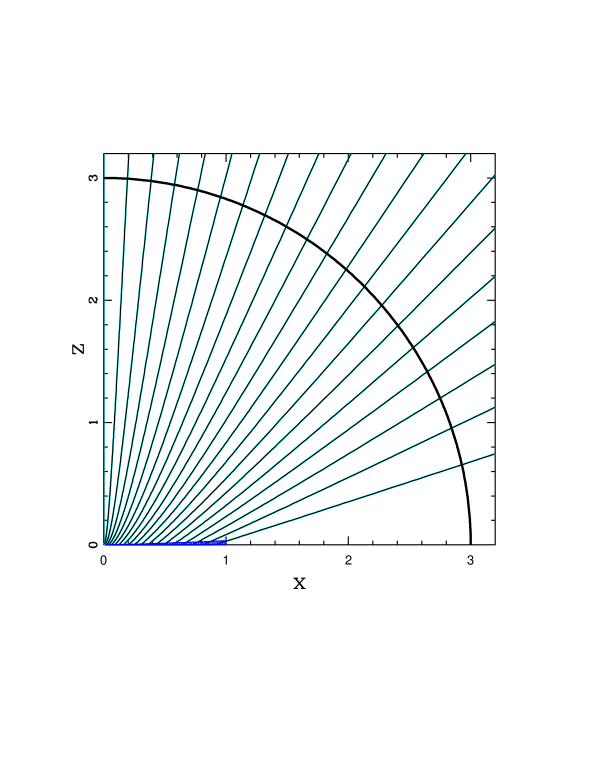
Figure 1: Projected trajectories of incoming parcels of gas falling toward the planet and its growing circumplanetary disk. The collection of trajectories corresponds to equally spaced initial values of $\sin\theta_{0}=0.05n$ (for integers $n$ = 0 – 19). The length scales are given in units of the centrifugal radius $R_{C}$. The disk, with radius $R_{\rm d}=R_{C}$, is depicted as the thin blue shaded region. The solid black curve at radius $r=3$ marks the Hill radius $R_{H}$. On this scale, the planet radius $R_{\rm p}\approx 0.006$.

The projected trajectories of the incoming parcels of gas are depicted in Figure 1. The initial (outer boundary) conditions for the trajectories are evenly spaced in $\sin\theta_{0}$. Note that the trajectories pass through the midplane ($z=0$) of the system before reaching their periastron point. Since we assume that the system has reflection symmetry about the $z=0$ plane, for each parcel of gas passing through the midplane from above, there will be a corresponding parcel passing through from below. These gas parcels will collide and shock, and thereby form a circumplanetary disk in the equatorial plane (delineated as the thin blue structure in the region $0\leq{x}\leq 1$ in the figure). Notice that the trajectories shown in Figure 1 are projected onto the meridional plane. The full three dimensional trajectories include an azimuthal component, so that the paths spiral around the rotational pole of the system as they move inward. This picture compares well with results found previously using numerical simulations (e.g., see Figure 4 of Tanigawa et al. 2012).

The above analysis provides a two dimensional description of the density distribution. It is sometimes useful to find an equivalent spherical infall region (Adams & Shu 1986; Section 5) by averaging the density distribution over the polar angle $\theta$ (equivalently, over $\mu$). The resulting density profile takes the form

$$\rho=Cr^{-3/2}{\cal A}(u)\,,$$ (13)

where the constant $C$ is defined by

$$C\equiv{{\dot{M}}_{\rm p}\over 4\pi\sqrt{2GM_{\rm p}}}\,,$$ (14)

and the asphericity factor ${\cal A}(u)$, with $u=r/R_{C}$, takes the form

$${\cal A}(u)=\sqrt{2u}\log\left[{1+\sqrt{2u}\over D(u)}\right]\qquad{\rm where}\qquad D(u)=\left\{\matrix{\sqrt{1-u}+\sqrt{u}&{\rm for}\,\,u<1\,;\cr$\,$&$\,$\cr\sqrt{2u-1}&{\rm for}\,\,u>1\,.}\right.$$ (15)

Note that ${\cal A}(u)\to 1$ in the limit of large radius $u\to\infty$ and that ${\cal A}(u)\to(2-\sqrt{2})u$ in the limit of small radius $u\to 0$. Notice also that this spherically averaged density distribution is not simply the density distribution that one would obtain from solving the spherically symmetric problem: Due to rotation and conservation of angular momentum, material does not fall as far inward, so that the density does not increase as rapidly in the limit $r\to 0$ (in this solution, compared to that for spherical collapse).

The column density through the infalling envelope plays an important role in determining the radiative signature of the forming planet (see Section 5). This column density is given by

$$N_{\rm col}=\int\rho dr=CR_{C}^{-1/2}\int u^{-3/2}{\cal A}(u)du\,.$$ (16)

If we take the limits of integration from 0 to $\infty$, the integral can be evaluated to obtain

$$N_{\rm col}={\sqrt{2}\pi^{2}\over 4}CR_{C}^{-1/2}\,.$$ (17)

For typical input parameters ($a=5$ AU, $M_{\rm p}=1M_{J}$, ${\dot{M}}_{\rm p}=1M_{J}$/Myr), the column density $N_{\rm col}\approx 0.05$ g cm^-2. Using a standard value of the dust opacity $\kappa_{V}=200$ cm² g^-1 (Draine & Lee, 1984), the visual extinction $A_{V}\approx 10$. However, the surface temperature of the planet is only $T_{\rm p}\sim 1000$ K, corrsesponding to wavelengths $\lambda\sim 3\mu$m, so that the optical depth of the envelope to the planetary radiation field is expected to be of order unity. As a result, only a modest fraction of the planetary luminosity will be absorbed by the infalling envelope and re-radiated at infrared wavelengths. Morever, the infrared extinction is less than unity, so that the envelope should be optically thin to the radiation it emits (see Section 5).

The column density is lowest along the rotational pole of the system, where $N_{\rm col}(\mu=0)=\pi CR_{C}^{-1/2}$, which is smaller than the equivalent spherical value by a factor of $\pi\sqrt{2}/4\sim 0.9$. The column density is larger along equatorial lines of sight, and becomes formally infinite in the limit $\mu=0$. In practice, however, this limit is not realized because the circumplanetary disk will retain a finite scale height. In addition, the equatorial lines of sight are blocked by the background circumstellar disk that surrounds the forming planet. We can also determine the corrections to the column density due to the finite inner cutoff at $r=R_{X}$ and the outer cutoff at $r=R_{H}$. Using the limiting forms for ${\cal A}(u)$ from equation (15), we find the contributions

$$\int_{0}^{R_{X}}\rho dr=CR_{C}^{-1/2}2(2-\sqrt{2})\sqrt{R_{\rm p}/R_{C}}\qquad{\rm and}\qquad\int_{R_{H}}^{\infty}\rho dr=CR_{C}^{-1/2}2\sqrt{3}/3\,.$$ (18)

The first correction is small (only $\sim 2.5\%$ of the total column density), whereas the second correction is more substantial ($\sim 1/3$ of the total). As a result, one should multiply the column density of equation (17) by a correction factor $(1-4\sqrt{6}/3\pi^{2})\approx 0.67$.

A related quantity is the mass of the infalling envelope at a given time in the development of the planet. The mass that is contained within the Hill sphere but has not reached the planet or disk is given by the integral

$$M_{\rm env}=\int_{R_{\rm p}}^{R_{H}}Cr^{-3/2}{\cal A}(u)4\pi r^{2}dr\approx\sqrt{6}{\dot{M}}_{\rm p}\Omega_{C}\,,$$ (19)

where $\Omega_{C}^{2}=GM_{\rm p}/R_{C}^{3}$. The ratio of the envelope mass to the planet mass is given by the ratio of the orbital period at the disk edge to the total planet formation time. We thus expect $M_{\rm env}/M_{\rm p}\sim 10^{-6}\ll 1$.

Note that the infalling envelope considered here is not in hydrostatic equilibrium, but rather is freely falling toward the central planet (and its disk) at the center of the flow. This configuration applies only to the final stage of giant planet formation when gas accretes rapidly, and when the planet gains most of its mass. In contrast, in the earlier stages, the material in this region is quasi-hydrostatic and must cool before it condenses toward the forming planet.

4 Circumplanetary Disk

This section outlines the formation and structure of the circumplanetary disk. As shown here, most of the material falls onto the disk, rather than directly onto the planet, so that disk accretion is an important feature of the process.

4.1 Infall onto the Disk

The rate at which the circumplanetary disk receives infalling material from the envelope is given by the density field and the velocity field. Using the results from the previous section, we obtain

$${d\Sigma\over dt}=2\rho v_{\theta}\Bigg{|}_{(r,\mu=0)}={{\dot{M}}_{\rm p}\over 2\pi r^{2}}{v_{\theta}\over|v_{r}|}{d\mu_{0}\over d\mu}={{\dot{M}}_{\rm p}\over 4\pi r^{2}}{1\over\zeta\mu_{0}}\,,$$ (20)

where all quantities are evaluated at the disk plane $(\mu=0)$. Note that the infall strikes the disk from both sides (top and bottom), leading to a factor of 2 in the result. Again using the orbit equation (5), the above expression can be evaluated to obtain

$${d\Sigma\over dt}={{\dot{M}}_{\rm p}\over 4\pi r^{2}}{1\over(\zeta^{2}-\zeta)^{1/2}}\,.$$ (21)

As a benchmark, it is useful to determine the surface density of the disk that would result in the absence of disk accretion (see the following section). This surface density is given by the integral of $d\Sigma/dt$ over time, equivalently mass, so that we obtain

$$\Sigma_{0}=\int{{\dot{M}}_{\rm p}dt\over 4\pi r^{2}}{1\over(\zeta^{2}-\zeta)^{1/2}}\,.$$ (22)

The subscript indicates that this surface density would result in the absence of viscous evolution $(\nu=0)$. Using $dM={\dot{M}}_{\rm p}dt$ and the definition of $\zeta$,

$$\zeta={R\over 3r}={a\over 3r}\left({M\over 3M_{\ast}}\right)^{1/3}\qquad\Rightarrow\qquad M=(3r/a)^{3}3M_{\ast}\zeta^{3}\,,$$ (23)

we find

$$\Sigma_{0}={243M_{\ast}r\over 4\pi a^{3}}\int{\zeta^{2}d\zeta\over(\zeta^{2}-\zeta)^{1/2}}\,.$$ (24)

Next we change variables to $u$ defined such that $u=1/\zeta$, so that the limits of integration are $u=3r/R_{H}$ and $u=1$. The resulting integral can be evaluated to obtain

$$\Sigma_{0}={3M_{\rm p}\over 16\pi R_{C}^{2}}\left\{{\sqrt{1-u}(2+3u)\over u}+3u\tanh^{-1}(\sqrt{1-u})\right\}\,.$$ (25)

Once the circumplanetary disk has become well-developed, the first term in the above expression dominates, and the surface density can be written in the approximate form

$$\Sigma_{0}\approx{3M_{\rm p}\over 8\pi R_{C}r}\,.$$ (26)

The enclosed mass thus has the radial dependence $M(r)\propto{r}$. As a result, most of the mass enters the planet/disk system at large radii $r\gg R_{\rm p}$, which in turn implies that disk accretion must be crucial for forming planets.

Figure 1 shows how the (projected) infalling trajectories of the flow join onto the circumplanetary disk. The inward paths are nearly radial at large distances $r>R_{C}$ (note that the length scales in the figure are given in units of the centrifugal radius $R_{C}=R_{H}/3$). In the inner regime, however, the trajectories depart significantly from radial paths, crossing the midplane and joining the disk well before reaching the planetary surface. Most of the incoming trajectories thus intercept the disk, rather than the planetary surface (which corresponds to $x\approx 0.006$ in the figure).

For completeness, we note that the solution (25) for the surface density assumes that infall takes place over all initial polar angles $\theta_{0}$. If infall is confined to the polar regions, as indicated by some numerical treatments (e.g., Lambrechts & Lega 2017; Lambrechts et al. 2019) then the centrifugal barrier $R_{C}$ will be smaller and the resulting surface density distribution will be steeper (see Fung et al. 2019). This modification, considering only the range $0\leq\theta_{0}\leq\theta_{max}$, is easily incorporated into this analytic treatment. On the other hand, viscous evolution will act to spread out the disk, increase its radius, and make the surface density distribution less steep, as shown in the following section.

4.2 Steady State Disk Evolution

Once the material has fallen onto the circumplanetary disk, its subsequent evolution occurs through viscous dissipation. Following standard nomenclature (Hartmann, 2009), we write the viscosity in the form

$$\nu=\alpha c_{s}H=\alpha c_{s}^{2}/\Omega\,.$$ (27)

Note that disk evolution for planet formation lies in a different regime than for star formation. The relevant quantity is the ratio of the viscous time scale to the accretion time scale, i.e.,

$${\cal R}={R^{2}\over\nu}{{\dot{M}}\over M}={1\over\alpha}{R^{2}\over H^{2}}{{\dot{M}}P\over 2\pi M}\sim{100\over 2\pi\alpha}{{\dot{M}}P\over M}\,,$$ (28)

where $P$ is the orbit time at the outer disk edge and where the final approximate equality assumes $H\sim R/10$. For star formation, $R\sim 100$ AU, $M=M_{\ast}\sim 1M_{\odot}$, $P\sim 1000$ yr, and $M_{\ast}/{\dot{M}}\sim 10^{5}$ yr. As a result, the ratio ${\cal R}_{\rm sf}\sim 1/2\pi\alpha$. For planet formation, $M_{\rm p}/{\dot{M}}_{\rm p}\sim 1$ Myr, whereas $P\sim 1$ yr, so that ${\cal R}_{\rm pf}\sim 10^{-4}/2\pi\alpha$. A much smaller viscosity is required for a planet forming disk to keep up with the infall compared to a star forming disk.

The equation of motion for a viscous accretion disk, including the infall terms derived in the previous section, can be written as

$${\partial\Sigma\over\partial t}={3\over r}{\partial\over\partial r}\left[r^{1/2}{\partial\over\partial r}\left(r^{1/2}\nu\Sigma\right)\right]+{{\dot{M}}_{\rm p}\over 4\pi r^{2}}{1\over(\zeta^{2}-\zeta)^{1/2}}\,.$$ (29)

In steady state, corresponding to vanishing time derivitives, the solution takes the from

$$\Sigma(r)={{\dot{M}}_{\rm p}\over 6\pi\nu}{1\over\sqrt{u}}\left[\sin^{-1}\sqrt{u}+\sqrt{u(1-u)}\right]={{\dot{M}}_{\rm p}\over 6\pi\nu}f(u)\,,$$ (30)

where $u\equiv r/R_{C}$ and where the second equality defines the function $f(u)$, which is of order unity and slowly varying with radius. Specifically, we note that the function $f\to 2$ in the inner limit $u\to 0$ and $f\to\pi/2$ in the outer limit $u\to 1$.

The diffusion equation has an additional solution, equivalently, an additional term, which has the form

$$\nu\Sigma={K_{1}\over r^{1/2}}+K_{2}\,,$$ (31)

where the $K_{j}$ are integration constants which can be chosen to satisfy the inner boundary condition. For stellar accretion disks, the usual assumption is to let $\nu\Sigma\to 0$ at the inner boundary. If we use this inner boundary condition, the full solution can be written in the form

$$\Sigma(r)={{\dot{M}}_{\rm p}\over 6\pi\nu}\left[f(u)-f(u_{\rm p})\left({u_{\rm p}\over u}\right)^{1/2}\right]\,,$$ (32)

where $u_{\rm p}\equiv R_{\rm p}/R_{C}$. The second term is negligible except near the surface of the planet. Moreover, in the present application, the disk is magnetically truncated so that the effective inner disk edge is well outside the planetary surface (see Section 4.3).

We can integrate the steady-state surface density over the disk area to find the disk mass,

$$M_{\rm d}={{\dot{M}}_{\rm p}\over 3}\int_{0}^{R_{C}}{rdr\over\nu}{1\over\sqrt{u}}\left[\sin^{-1}\sqrt{u}+\sqrt{u(1-u)}\right]\,.$$ (33)

If we assume that the temperature within the disk scales as $T\sim r^{-1/2}$, then $\nu\sim r$, so that we can write $\nu=\nu_{C}(r/R_{C})=\nu_{C}u$. The disk integral then becomes

$$M_{\rm d}={{\dot{M}}_{\rm p}R_{C}^{2}\over 3\nu_{C}}\int_{0}^{1}{du\over\sqrt{u}}\left[\sin^{-1}\sqrt{u}+\sqrt{u(1-u)}\right]={{\dot{M}}_{\rm p}R_{C}^{2}\over 3\nu_{C}}\left[\pi-{4\over 3}\right]\,.$$ (34)

We thus find that $M_{\rm d}/M_{\rm p}\sim{\cal R}$ from equation (28) as expected.

With the steady-state solution in place, we can now consider how the disk evolves into such a configuration. The steady-state disk arises when the two terms on the right hand side of equation (29) are in balance. At the onset of disk formation, however, the viscous term is small (compared to the infall term) because the surface density must be small. In this regime, the surface density of the disk builds up mass from infall as described in the previous section. The surface density will grow until it becomes comparable to the steady-state solution, where the required time for this transient growth is determined by viscosity so that $\Delta{t}\sim{R_{C}^{2}}/\nu_{C}$. Since the viscous time scale is much shorter than the evolutionary time scale (equation [28]), the disk surface density has the steady-state form for most of its lifetime. For completeness, note that the centrifugal radius $R_{C}$ grows with increasing planet mass with the scaling law $R_{C}\sim M_{\rm p}^{1/3}$. The weak dependence of $R_{C}$ on mass implies that $R_{C}$ varies only weakly with time, so that the evolution of disk surface density can be separated into the regimes described above.

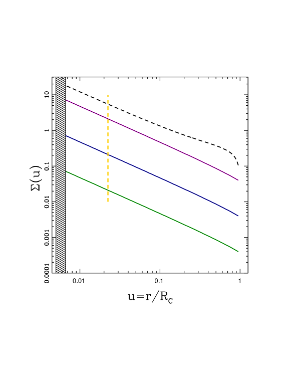
Figure 2: Surface density distributions for circumplanetary disks forming through infall from the circumstellar disk. The black dashed curve shows the normalized surface density profile in the absence of viscous evolution, where infalling material is assumed to stay at the radial location where it crosses the midplane. The three solid curves show the normalized steady-state surface density distributions for viscous parameters $\alpha$ = $10^{-4}$ (upper, magenta), $10^{-3}$ (middle, blue), and $10^{-2}$ (lower, green). The hatched region on the left represents the planetary surface. The vertical dashed orange line delineates the expected location of the magnetic truncation radius and hence the effective inner boundary of the disk.

4.3 Magnetic Truncation at the Inner Boundary

With the outer boundary of the disk specified, we need to consider the inner boundary. In the absence of planetary magnetic fields, the circumplanetary disks can extend all the way to the planet’s surface. In general, however, we expect the planet to develop a strong internal magnetic field with surface strength $B_{\rm p}$ (see Appendix B for an estimate). To leading order, such fields have a dipole form,

$$B(r,\theta)=B_{\rm p}\left({R_{\rm p}\over r}\right)^{3}\left[3\cos\theta{\hat{r}}-{\hat{z}}\right]\,,$$ (35)

where the spherical coordinate system is centered on the planet. The incoming flow from the circumplanetary disk cannot penetrate past the point where the ram pressure of the inward flow is balanced by the outward pressure from the magnetic field. This magnetic truncation radius has the form

$$R_{X}=\omega\left({B_{\rm p}^{4}R_{\rm p}^{12}\over GM_{\rm p}{\dot{M}}_{\rm p}^{2}}\right)^{1/7}\,,$$ (36)

where $\omega$ is a dimensionless constant of order unity (Ghosh & Lamb 1978; Blandford & Payne 1982; see also the discussion of Mohanty & Shu 2008 for an alternate derivation).

If we insert typical numbers, the truncation radius can be evaluated to find:

$${R_{X}\over R_{\rm p}}\approx 3.8\left({M_{\rm p}\over M_{J}}\right)^{-1/7}\left({{\dot{M}}_{\rm p}\over 1\,M_{J}\,/\,{\rm Myr}}\right)^{-2/7}\left({B_{\rm p}\over 500\,\,{\rm gauss}}\right)^{4/7}\left({R_{\rm p}\over 10^{10}\,\,{\rm cm}}\right)^{5/7}\,.$$ (37)

For comparison, the centrifugal radius, and hence the disk radius, is given by

$$R_{\rm d}=R_{C}={R_{H}\over 3}\qquad\Rightarrow\qquad{R_{\rm d}\over R_{\rm p}}\approx 170\left({M_{\rm p}\over M_{J}}\right)^{1/3}\left({a\over 5{\rm AU}}\right)\,.$$ (38)

Since the disk radius scales as with the semimajor axis, planets forming in the inner regions of the circumstellar disk have radially small infall regions and produce radially small circumplanetary disks. For standard parameters, the magnetic truncation radius is larger than the disk radius for planets forming at semimajor axes $a\,\raise 1.29167pt\hbox{$<$}\kern-7.5pt\lower 3.01385pt\hbox{$\sim$}\,0.1$ AU. As a result, magnetic fields could represent a significant obstacle to forming giant planets near their host stars. For completeness, we can write the condition $R_{X}=R_{C}$ in the form

$$\left({a\over R_{\rm p}}\right)\left({M_{\rm p}\over M_{\ast}}\right)^{10/21}=3^{4/3}\omega\left({B_{\rm p}^{4}R_{\rm p}^{5}\over GM_{\ast}{\dot{M}}_{\rm p}^{2}}\right)^{1/7}\,.$$ (39)

4.4 Disk Structure

The previous subsections define the expected structure for the circumplanetary disks that arise during the process of planet formation. The surface densities for these disks are shown in Figure 2. The upper black dashed curve shows the surface density profile that would result in the absence of viscous accretion (as derived in Section 4.1). The surface density shows a radial dependence of the approximate form $\Sigma\propto 1/r$, except near the outer edge where an enhancement is present, followed by a sharp edge at $r=R_{C}$. In the presence of viscosity, the disk surface density is given by the steady-state solutions of Section 4.2. Surface density profiles are shown in the figure for $\alpha$ = $10^{-2}$, $10^{-3}$, and $10^{-4}$, from bottom to top. The larger viscosity results in lower disks masses in steady state. The surface density profiles are normalized by dividing out a factor of $M_{\rm p}/R_{C}^{2}$, where $M_{\rm p}$ represents the total mass that has fallen to the planet/disk system. For the viscous models, we further specify the mass infall rate to be $1M_{J}$/Myr and the radial location of the planet to be $a$ = 5 AU. With these choices, for a planet with mass $M_{\rm p}=1M_{J}$, the circumplanetary disk has outer radius $R_{C}/R_{\rm p}=170$ and an inner boundary given by the magnetic truncation radius at $R_{X}/R_{\rm p}=3.8$, as depicted by the vertical orange dashed line in Figure 2. Although the surface density profiles are truncated at $r=R_{C}$ in the figure, the solutions can be extended beyond this nominal disk radius where they match onto more steeply decreasing profiles (see Appendix D). Note that the disk must spread beyond $R_{C}$ in order to satisfy conservation of angular momentum.

The circumplanetary disks thus have relatively simple forms. The dynamic range is small, with $R_{C}/R_{X}\sim 40-50$. The disk masses are a small fraction of the total mass (equation [34]) and the surface density distribution is close to a $1/r$ power-law (equation [30]). In spite of the small disk masses, the surface densities are large enough for the disks to remain optically thick to their internal infared radiation.

4.5 Planet Masses without Disk Accretion

Before leaving this section, it is useful to consider how gaseous planets would form in the absence of disk accretion (through the circumplanetary disk). If the viscosity vanishes, $\nu\to 0$, then the rate at which the planet gains mass is limited by the geometry of the infall and has the form

$${\dot{M}}_{\rm p}\Big{|}_{direct}=4\pi R_{\rm p}^{2}\int_{0}^{1}\rho|v_{r}|d\mu\,,$$ (40)

where the integrand is evaluated at the planetary surface. Using the infall solution from Section 3 (see also Adams & Shu 1986 for the star formation analog), we can evaluate the integral to obtain

$${\dot{M}}_{\rm p}\Big{|}_{direct}={\dot{M}}_{\rm p}\left[1-\sqrt{1-R_{\rm p}/R_{C}}\right]\,.$$ (41)

The rate of accretion onto the planet is thus an ever-decreasing fraction of the total infall rate.

The planet mass $M_{\rm p}$ for a given mass $M$ that has fallen is given by the integral expression

$$M_{\rm p}=M_{0}+\int_{M_{0}}^{M}dM\left[1-\sqrt{1-(M_{0}/M)^{1/3}}\right]\,,$$ (42)

where the scale $M_{0}$ is the mass for which the centrifugal radius is equal to the planetary radius, i.e.,

$$M_{0}=81M_{\ast}\left({R_{\rm p}\over a}\right)^{3}\,.$$ (43)

For planets forming at $a\sim 5$ AU, $M_{0}\sim 2\times 10^{-7}$ $M_{J}$. In contrast, for hot Jupiters at $a=0.05$ AU, $M_{0}\sim 0.2M_{J}$. For both scenarios, the formation of a Jovian-mass planet requires accretion via a circumplanetary disk. For cold Jupiters, the vast majority of the mass must be accreted through the disk. For hot Jupiters, however, a significant fraction of the mass can be accreted directly (notice also that hot Jupiters tend to have somewhat smaller masses).

Note that the above treatment does not include the effects of planetary magnetic fields, which act to increase the effective capture cross section of the growing planet. For a given estimate of the effective capture radius $R_{\sigma}$ (see Section 4.6) one can replace $R_{\rm p}$ with $R_{\sigma}$ in the above expressions.

A related question is: How much total mass must flow through the Hill sphere in order for a given mass to directly accrete onto the planet? We can evaluate equation (42) in the asymptotic limit $M\gg M_{0}$ to obtain

$$M_{\rm p}\to{3\over 4}\left(M_{0}M^{2}\right)^{1/3}\,.$$ (44)

In order to produce a final planet mass of $M_{\rm p}=1M_{J}$ (with no circumplanetary disk accretion and at radial location $a=5$ AU), we would need a total mass $M\approx 3400M_{J}=3.4M_{\odot}$. In other words, in order for a Jovian mass to fall directly to the planet, several stellar masses of material must cycle through the Hill sphere. Some mechanism for redistributing angular momentum — within the sphere of influence of the forming object — is thus necessary for the formation of Jovian planets. Viscosity in the circumplanetary disk provides such a mechanism for the scenario explored in this paper.

4.6 Magnetic Capture Radius

The magnetic truncation radius $R_{X}$ (equation [36]), which arises from the balance between disk accretion and magnetic pressure, defines the inner edge of the circumplanetary disk. However, for material falling onto the system near the rotational poles, a second magnetic boundary $R_{\sigma}$ arises from the balance between the ram pressure of infalling material and the magnetic pressure. These two scales are different because not all of the infalling material can reach inner radii comparable to the planetary size, so that the mass infall rate is reduced and the boundary is larger. Equating the incoming ram pressure $\rho v^{2}$ with the magnetic field pressure at the pole ($\mu=1$), we can write the magnetic capture radius in the form

$${R_{\sigma}\over R_{\rm p}}={\tilde{\omega}}\left({B_{\rm p}^{4}R_{\rm p}^{3}R_{C}^{2}\over GM_{\rm p}{\dot{M}}_{\rm p}^{2}}\right)^{1/9}\,,$$ (45)

where ${\tilde{\omega}}$ is a dimensionless constant of order unity and where the quantity ${\dot{M}}_{\rm p}$ is the total mass accretion rate. For typical parameter values, the capture radius is somewhat larger than the disk truncation radius so that $R_{\sigma}\sim 1.4R_{X}$ (compare with equation [36]).

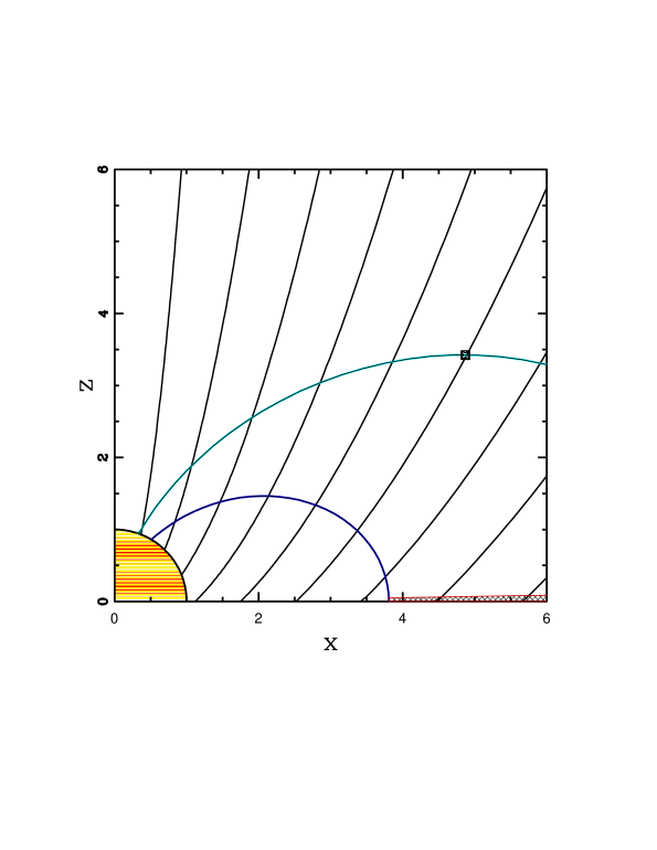
Figure 3: Inner infall region near the planet (for mass $M_{\rm p}=1M_{J}$, accretion rate ${\dot{M}}_{\rm p}=1M_{J}$/Myr, and field strength $B_{\rm p}=500$ gauss). The black solid curves show the projected incoming trajectories for parcels of gas with starting conditions near the pole. The planet is depicted as the (partial) circular region in the lower left. Two magnetic field lines are shown, with the lower blue curve connecting to the magnetic truncation radius $R_{X}$ of the disk (in the equatorial plane) and the upper cyan curve defining the capture radius $R_{\sigma}$, (marked by the square symbol). The horizontal point of the upper curve, $x_{\rm hor}=R_{\sigma}\sin\theta$, is roughly coincident with the disk truncation radius defined by the lower curve. The length scales are given in units of the planetary radius $R_{\rm p}$, so that the disk radius $R_{\rm d}=R_{C}\approx 180$ and the Hill radius $R_{H}\approx 540$.

The magnetic field lines and incoming trajectories near the forming planet are shown in Figure 3. Keep in mind that all of the trajectories in the figure correspond to small values of the initial polar angle $\theta$ (otherwise the trajectories would cross the plane of the disk far to the right). In order for an incoming parcel of gas to be deflected by the magnetic fields, its radial location is given by equation (45). In order for the parcel to subsequently move inward onto the planet, rather than outward and back towards the disk, it must fall sufficiently close to the pole. Here we approximate this bifurcation point as the point where the magnetic field line is horizontal and where the magnetic pressure balances the ram pressure. This critical point of the field line corresponds to the location where the horizontal coordinate has the form

$$x_{\rm hor}=\left({2\over 3}\right)^{1/2}R_{\sigma}\sim 0.82R_{\sigma}\,.$$ (46)

We thus have the following result: The capture radius $R_{\sigma}$ is larger than the magnetic truncation radius because the direct infall is reduced in the inner region. However, only the innermost portion of the capture region funnels material directly onto the planet rather than outward and onto the disk (see Batygin 2018; Batygin & Morbidelli 2020). The radius $R_{\sigma}$ is somewhat larger than $R_{X}$ and $x_{\rm hor}$ is somewhat smaller than $R_{\sigma}$, so that the two corrections tend to compensate. In the end, the effective capture cross section is given approximately by the length scale $R_{X}$.

5 Radiative Signatures

With the properties of the infalling envelope and the circumplanetary disk specified, we can now estimate the accretion luminosity of the central planet/disk system and the corresponding spectral energy distributions.

5.1 Luminosity Contributions from the Planet and its Disk

Since most of the mass falling onto the planet/disk system is eventually accreted onto the growing planet, the luminosity contributions can be written in terms of the benchmark power scale

$$L_{0}\equiv{GM_{\rm p}{\dot{M}}_{\rm p}\over R_{\rm p}}\,,$$ (47)

which corresponds to the total power that could be generated if all of the incoming material falls (from rest at infinity) onto the planetary surface at free-fall speeds and dissipates all of its kinetic energy.

The luminosity of the system is distributed between the planet and its disk. Only a fraction $f_{\rm p}$ of the incoming material falls directly onto the planet (see equation [41]). However, an additional fraction of the material falls within the magnetic capture radius (Section 4.6) and is funneled onto the planet along magnetic field lines. The remaining incoming material falls onto the disk. For the sake of definiteness and simplicity, we assume that the magnetic truncation radius $R_{X}$ of the disk and the magnetic capture radius $R_{\sigma}$ are equal. The fractions of the incoming material that fall onto the planet and onto the disk are thus given by

$$f_{\rm p}=1-\sqrt{1-u_{\rm x}}\qquad{\rm and}\qquad f_{\rm d}=\sqrt{1-u_{\rm x}}\,,$$ (48)

where we have defined $u_{\rm x}\equiv R_{X}/R_{C}$. If the planetary magnetic field is sufficiently weak, so that $R_{X}\leq R_{\rm p}$, then $u_{\rm x}=R_{\rm p}/R_{C}$.

To specify the planetary component of the accretion luminosity, we assume that all of the material that falls within the capture radius is accreted by the planet, and that shocks on the surface dissipate the radial and poloidal components of the velocity. The planet is assumed to be co-rotating with its disk at the magnetic truncation point, so that the planetary rotation rate is given by

$$\Omega_{\rm p}^{2}={GM_{\rm p}\over R_{X}^{3}}\,.$$ (49)

The incoming material thus retains a small azimuthal velocity given by $v_{\phi}=\sin\theta R_{\rm p}\Omega_{\rm p}$. The luminosity thus takes the form

$$L_{\rm p}^{\rm dir}=\left(1-\sqrt{1-u_{\rm x}}\right)\left(1-{1\over 2}\langle\sin^{2}\theta\rangle{R_{\rm p}^{3}\over R_{X}^{3}}\right)L_{0}\,,$$ (50)

where the angular brackets represent an average over the co-latitudes. The newly added material is eventually distributed over the planetary surface, so we expect $\langle\sin^{2}\theta\rangle\approx 2/3$.

Although the remaining fraction of the material falls onto the disk, it eventually accretes onto the planet. However, it falls from the magnetic truncation radius, rather than from infinity, so that the additional planetary luminosity derived from accretion takes the approximate form

$$L_{\rm p}^{\rm acc}=L_{0}\sqrt{1-u_{\rm x}}\left(1-{R_{\rm p}\over R_{X}}\right)\left(1-{R_{\rm p}^{3}\over 3R_{X}^{3}}\right)\,.$$ (51)

As written, the expression has three correction factors: The first determines the amount of material that falls onto the disk (the remaining fraction is accounted for in the previous contribution). The second factor takes into account the starting point for the material, which falls from an initial radius $R_{X}$ instead of $r\to\infty$. The third factor takes into account the rotational motion of the incoming material, where we again assume that the magnetic field causes the incoming material to rotate with the mean motion of the disk at the location $R_{X}$ and that the incoming material is uniformly distributed in planetary latitude. Although this correction factor is close to unity, note that other assumptions can be invoked. For completeness, we note that the planet and its disk could support outflows or winds analogous to those observed in young stellar objects. Such winds could result in a reduced accretion rate onto the planetary surface, and could play a role in redistributing angular momentum. Although potentially important, we leave this issue for future work.

The luminosity contributions from both direct infall and from the inner edge of the disk combine to determine the total planetary accretion luminosity $L_{\rm p}$, which takes the form

$$L_{\rm p}=\left(1-\sqrt{1-u_{\rm x}}{R_{\rm p}\over R_{X}}\right)\left(1-{R_{\rm p}^{3}\over 3R_{X}^{3}}\right)L_{0}\,.$$ (52)

In general, the planet has an additional internal luminosity $L_{\rm int}$, although the accretion luminosity is expected to be somewhat larger (see, e.g., Marley et al. 2007). The planet must radiate the total luminosity, given by equation (52) and $L_{\rm int}$, and has an effective surface temperature given by

$$\sigma T_{\rm p}^{4}={L_{0}\over 4\pi R_{\rm p}^{2}}\left(1-\sqrt{1-u_{\rm x}}{R_{\rm p}\over R_{X}}\right)\left(1-{R_{\rm p}^{3}\over 3R_{X}^{3}}\right)+{L_{\rm int}\over 4\pi R_{\rm p}^{2}}\,.$$ (53)

In the limit $L_{\rm int}\to 0$, only the first term contributes, and we make this approximation for the rest of this paper.

The remainder of the energy is dissipated within the disk, which has total luminosity given by

$$L_{\rm d}=L_{0}{R_{\rm p}\over 2R_{X}}\sqrt{1-u_{\rm x}}\,,$$ (54)

where the factor of 2 arises because half of the energy is stored in rotational energy of the disk. Because the magnetic truncation radius is typically $R_{X}\sim 4R_{\rm p}$, the total accretion luminosity generated on the planetary surface is larger than the disk luminosity by (about) an order of magnitude. From the perspective of the infalling envelope, most of the energy is generated by a point source in the center of the structure.

The total disk luminosity is distributed among three components: The perpendicular component $v_{\theta}$ of the incoming velocity is dissipated as it strikes the disk, thereby producing luminosity $L_{\rm d}^{\rm surf}$. When the material reaches the disk, however, it generally will not have the right azimuthal velocity to enter into Keplerian rotation about the planet. The new material thus mixes with existing disk material, dissipates energy while conserving angular momentum, and produces a mixing luminosity $L_{\rm d}^{\rm mix}$. The remaining luminosity $L_{\rm d}^{\rm visc}$ must be dissipated (in this approximation) by the viscosity. The surface and mixing contributions for circumstellar disks have been calculated previously (Cassen & Moosman, 1981; Cassen & Summers, 1981; Adams & Shu, 1986) and can be written in the form

$$L_{\rm d}^{\rm surf}=\int_{A}\left({1\over 2}v_{\theta}^{2}\right)\rho|v_{\theta}|dA={u_{\rm x}\over 4}\left\{\ln\left[{1+\sqrt{1-u_{\rm x}}\over 1-\sqrt{1-u_{\rm x}}}\right]-2\sqrt{1-u_{\rm x}}\right\}L_{0}\,,$$ (55)

and

$$L_{\rm d}^{\rm mix}=\int_{A}{1\over 2}\left\{v_{r}^{2}+\left[v_{\phi}-\left({GM_{\rm p}\over r}\right)^{1/2}\right]^{2}\right\}\rho|v_{\theta}|dA$$

$$={u_{\rm x}\over 2}\left\{\ln\left[{1+\sqrt{1-u_{\rm x}}\over 1-\sqrt{1-u_{\rm x}}}\right]+\sqrt{1-u_{\rm x}}+\pi-2\tan^{-1}\left[{u_{\rm x}\over 1-u_{\rm x}}\right]^{1/2}\right\}L_{0}\,.$$ (56)

These two luminosity contributions (see also Szulágyi & Mordasini 2017) represent the energy that is dissipated as material joins the disk, independent of any subsequent viscous evolution, and can be combined to define a total direct luminosity contribution $L_{\rm d}^{\rm dir}$ = $L_{\rm d}^{\rm surf}+$ $L_{\rm d}^{\rm mix}$, i.e.,

$$L_{\rm d}^{\rm dir}={u_{\rm x}\over 4}\left\{3\ln\left[{1+\sqrt{1-u_{\rm x}}\over 1-\sqrt{1-u_{\rm x}}}\right]+2\pi-4\sin^{-1}\sqrt{u_{\rm x}}\right\}L_{0}\,.$$ (57)

In the limit where all of the material can be accreted onto the planet, the remaining viscous luminosity is given by

$$L_{\rm d}^{\rm visc}=L_{\rm d}-L_{\rm d}^{\rm dir}\,.$$ (58)

Although we can separate the contributions to the disk luminosity, the net result of viscous evolution is to transport all of the incoming material inward to the magnetic truncation radius. As a result, the total disk luminosity has the simple form given by equation (54). We can approximate the temperature distribution from the disk surface using the form

$$T_{\rm d}(r)=T_{X}\left({R_{X}\over r}\right)^{3/4}\,,$$ (59)

where the leading coefficient is determined by the requirement that the disk radiates its total luminosity,

$$\sigma T_{X}^{4}={GM_{\rm p}{\dot{M}}_{\rm p}\over 8\pi R_{X}^{3}}{1\over\sqrt{1-u_{\rm x}}}\,.$$ (60)

Note that the power-law dependence of the temperature distribution (59) does not continue to arbitrarily large radii. The forming planet is embedded within the circumstellar disk of its host star, and this nebula provides a background minimum temperature for the circumplanetary disk.

With the surface temperatures of the planet and the disk specified, we can define the corresponding spectral energy distributions of the two central components

$$L_{{\rm p}\nu}=4\pi R_{\rm p}^{2}\pi B_{\nu}(T_{\rm p})\,,$$ (61)

and

$$L_{{\rm d}\nu}=2(2\cos\theta)\int_{R_{X}}^{R_{C}}\pi B_{\nu}[T_{\rm d}(r)]2\pi rdr\,.$$ (62)

The leading factor of 2 arises because the disk has two sides and the factor of $(2\cos\theta)$ arises from the viewing angle. Here we have assumed that the disk is optically thick to its own emission and this expression does not include external extinction (see also Zhu 2015; Zhu et al. 2018). The corresponding monochromatic fluxes arising from the planet and its disk have the form

$$F_{{\rm p}\nu}(r,\mu)={L_{{\rm p}\nu}\over 4\pi r^{2}}G_{\rm pd}(\mu)\exp[-\tau_{\nu}(r,\mu)]\,,$$ (63)

and

$$F_{{\rm d}\nu}(r,\mu)={L_{{\rm d}\nu}\over 4\pi r^{2}}(2\mu)G_{\rm dp}(\mu)\exp[-\tau_{\nu}(r,\mu)]\,,$$ (64)

as seen by an observer with location $(r,\mu)$. The optical depth of the infalling envelope $\tau_{\nu}$ depends on the viewing angle. For completeness, we include the functions $G_{\rm dp}(\mu)$ and $G_{\rm pd}(\mu)$, which take into account the mutual shadowing of the planet by the disk, and the disk by the planet (Adams & Shu, 1986). Most of the shadowing takes place near the planet, however, and we expect the magnetic truncation radius to remove the nearest disk material, so that the shadowing factors are close to unity in the present application.

5.2 Radiation from the Circumplanetary Envelope

Here we consider the infalling envelope surrounding the forming planet to be optically thin to its own emitted thermal photons. In this limit, the spectral energy ${\cal L}_{\nu}$ corresponding to dust emission has the form

$${\cal L}_{\nu}=f_{e}\int_{R_{X}}^{R_{H}}\rho\kappa_{\nu}4\pi B_{\nu}(T)\,4\pi r^{2}dr\,,$$ (65)

where $\kappa_{\nu}$ is the frequency dependent opacity and $B_{\nu}$ is the Planck function. The magnetic truncation radius $R_{X}$ delineates the inner boundary of the envelope and the Hill radius $R_{H}$ marks the outer boundary of the infall region. We are thus implicitly assuming that the radiation field reaches its eventual free-streaming form for $r\,\raise 1.29167pt\hbox{$<$}\kern-7.5pt\lower 3.01385pt\hbox{$\sim$}\,R_{H}$. The factor $f_{e}\leq 1$ represents a covering fraction, which allows for a possible reduction in the solid angle subtended by the envelope, with a corresponding reduction in the emitted radiation (although we take $f_{e}=1$ for the sake of definiteness). The density distribution is that found in Section 3, where we use the equivalent spherical distribution for simplicity.

The interaction between the radiation field and the envelope is dominated by the dust opacity $\kappa_{\nu}$. Although the dust opacity in the interstellar medium has been well characterized (starting with Draine & Lee 1984), the dust within circumstellar disks is expected to evolve significantly from its interstellar form. Dust grains generally grow, and opacity decreases as the grain size becomes comparable to the wavelength of the radiation. In the present context, the temperature of the envelope falls in the range 100 K $\leq{T}\leq$ 1000 K. Over this interval, the Planck mean and Rosseland mean opacities are slowly varying functions of temperature, and the different possible models are in relatively good agreement (e.g., see Semenov et al. 2003 and references therein). As a result, to a good approximation, we can consider the opacity to have the power-law form $\kappa_{\nu}=\kappa_{0}(\nu/\nu_{0})^{\eta}$. The Planck mean opacity then has the temperature dependence $\kappa_{P}=b_{\kappa}T^{\,\eta}$, where the constant $b_{\kappa}$ is given by

$$b_{\kappa}\equiv\kappa_{0}\left({k\over h\nu_{0}}\right)^{\eta}{\Gamma(4+\eta)\,\zeta_{\scriptscriptstyle R}(4+\eta))\over 6\,\zeta_{\scriptscriptstyle R}(4)}\,.$$ (66)

Here $k$ and $h$ are the Boltzmann and Planck constants, respectively, $\Gamma(z)$ is the gamma function and $\zeta_{\scriptscriptstyle R}(z)$ is the Riemann zeta function (Abramowitz & Stegun, 1972). With the choices $\eta=1$, $\kappa_{0}$ = 10 cm²/g, and $\nu_{0}=10^{14}$ Hertz, the resulting $\kappa_{\nu}$ is somewhat smaller than the interstellar opacity, but the resulting mean opacities are within the ranges advocated by Semenov et al. (2003) for circumstellar disks. We use these values for the results presented below, but they are readily varied given the analytical solutions developed herein.

As a further simplification, we note that the infalling envelope is optically thin to its emitted radiation field. In this regime, we can solve the radiative transfer equation (Adams & Shu, 1985) and find that the temperature profile takes the power-law form

$$T(r)=T_{C}\left({r\over R_{C}}\right)^{-2/5}\,,$$ (67)

where the power-law exponent is appropriate for the dust opacity law ($\kappa_{\nu}\propto\nu$) used above (in general, the exponent is $2/(\eta+4)$). With the temperature profile specified, we can evaluate the total luminosity emitted by the infalling envelope to find

$${\cal L}=16\pi\int_{R_{X}}^{R_{H}}\rho\kappa_{P}\sigma T^{4}r^{2}dr\,,$$ (68)

where $\kappa_{P}$ is the Planck mean opacity. The integral expression for the envelope luminosity ${\cal L}$ can be evaluated and has the form

$${\cal L}=16\pi\,\sigma\,Cb_{\kappa}T_{C}^{5}R_{C}^{3/2}\int_{u_{\rm x}}^{3}u^{-3/2}{\cal A}(u)du=16\pi R_{C}^{2}\,\sigma\,b_{\kappa}T_{C}^{5}N_{\rm col}\,.$$ (69)

Note that the upper limit of the integral in equation (69) is taken to be the outer boundary of the infalling envelope at $u=3$ (equivalently, $r=R_{H}$). The fiducial temperature $T_{C}$ is thus given by

$$T_{C}=\left({{\cal L}\over 16\pi R_{C}^{2}\sigma N_{\rm col}b_{\kappa}}\right)^{1/5}\,.$$ (70)

The total envelope luminosity ${\cal L}$ is determined by the fraction of the central source radiation that is attenuated by the infalling envelope,

$${\cal L}=\left[L_{\rm p}+L_{\rm d}-\int_{0}^{\infty}d\nu(L_{{\rm p}\nu}+L_{{\rm d}\nu})\exp(-\tau_{\nu})\right]\,,$$ (71)

where $\tau_{\nu}$ = $\kappa_{\nu}N_{\rm col}$ is the total optical depth through the envelope for a given frequency. For typical parameters, the fraction of the central source luminosity that is absorbed by the envelope is $\sim 0.25-0.5$, i.e., ${\cal L}\sim 0.25$ $(L_{\rm p}+L_{\rm d})$. The optical depth of the envelope to the central source radiation is thus of order unity. The optical depth of the envelope to its emitted radiation, which has longer wavelength, is much less than unity, so that the optically thin approximation is valid.

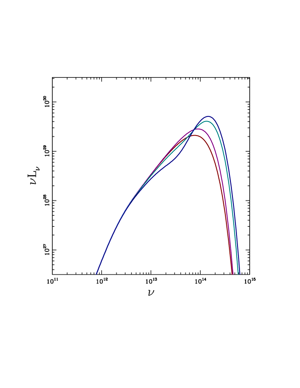
Figure 4: Spectral energy distributions of the central planet and its circumplanetary disk. The planet has mass $M_{\rm p}=1M_{J}$, mass accretion rate ${\dot{M}}_{\rm p}$ = $1M_{J}$/Myr, and radial location $a=5$ AU. Results are shown in the absence of extinction for a range of magnetic truncation radii, from $R_{X}=R_{P}$ out to $R_{X}\approx 5.6R_{P}$, corresponding to surface magnetic field strengths $B_{\rm p}$ = 10, $10^{3/2}$, 100, $10^{5/2}$, and 1000 gauss (from bottom to top). The frequency $\nu$ is given in Hertz, and spectral energy $\nu L_{\nu}$ is given in erg/s.

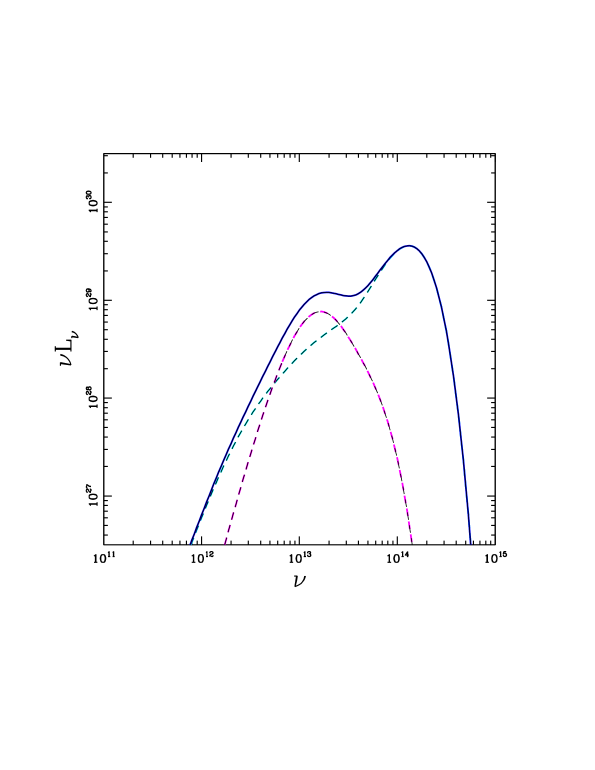
Figure 5: Emergent spectral energy distributions for a forming planet. The planet is assumed to have mass $M_{\rm p}=1M_{J}$, radial location $a$ = 5 AU, mass accretion rate ${\dot{M}}_{\rm p}$ = $1M_{J}$/Myr, and have surface magnetic field strength $B_{\rm p}=1000$ gauss. Emission from the central planet and disk is attenuated by the infalling envelope, with emergent spectral energy shown as the dashed cyan curve. Emission from the envelope itself is shown as the dashed magenta curve. The total spectral energy distribution is shown as the solid blue curve. (Frequency $\nu$ is in Hertz and spectral energy $\nu L_{\nu}$ is in erg/s.)

5.3 Spectral Energy Distributions

With the properties of the planet, disk, and infalling envelope specified, we can determine the spectral energy distribution of the forming planet. Here we present only a simple continuum model where the planetary surface and the disk surface are assumed to radiate as blackbodies. Future work should consider line emission.

The spectral energy distributions of the central planet/disk system are shown in Figure 4. The planet mass is taken to be $M_{\rm p}=1M_{J}$ with a mass accretion rate ${\dot{M}}_{\rm p}$ = $1M_{J}$/Myr. The planet is assumed to form at radial location $a$ = 5 AU, which determines its Hill radius and hence the disk radius. For a given choice of magnetic field strength on the planetary surface, the inner edge of the disk is determined by the magnetic trunaction radius. The curves shown in the Figure correspond to logarithmically spaced values in the range $B_{\rm p}$ = 10 – 1000 gauss (increasing from bottom to top). Stronger magnetic fields result in larger magnetic truncation radii $R_{X}$. Under the assumption of steady state disk accretion, larger values of $R_{X}$ result in larger overall luminosity and more accretion power generated on the planetary surface (see Section 5.1). Smaller inner radii $R_{X}$ allow for relatively more energy to be dissipated in the disk, rather than on the planetary surface, so that the spectral energy distributions become somewhat redder. The differences are modest, however, with the total luminosity varying by only a factor of $\sim 2$ over the given parameter range.

Radiation from the central planet/disk system is absorbed and re-radiated by the infalling envelope (Section 5.2). The total optical depth of the envelope to the central source photons is less than unity, so that only a fraction of the total luminosity is reprocessed. Figure 5 shows the resulting emergent spectral energy distribution for a typical system with mass $M_{\rm p}$ = 1 $M_{J}$, mass accretion rate ${\dot{M}}$ = 1 $M_{J}$/Myr, location $a=5$ AU, and magnetic field strength $B_{\rm p}=1000$ gauss (so that $R_{X}\approx 5.6$ $R_{\rm p}$). The contributions from the central source and the envelope are shown separately (dashed curves), with the total given by the solid curve. As expected, the envelope dominates the emission at sufficiently long wavelengths ($\lambda\sim 10$ $\mu$m), whereas more energy is emitted at shorter wavelengths ($\lambda\,\raise 1.29167pt\hbox{$<$}\kern-7.5pt\lower 3.01385pt\hbox{$\sim$}\,1$ $\mu$m).

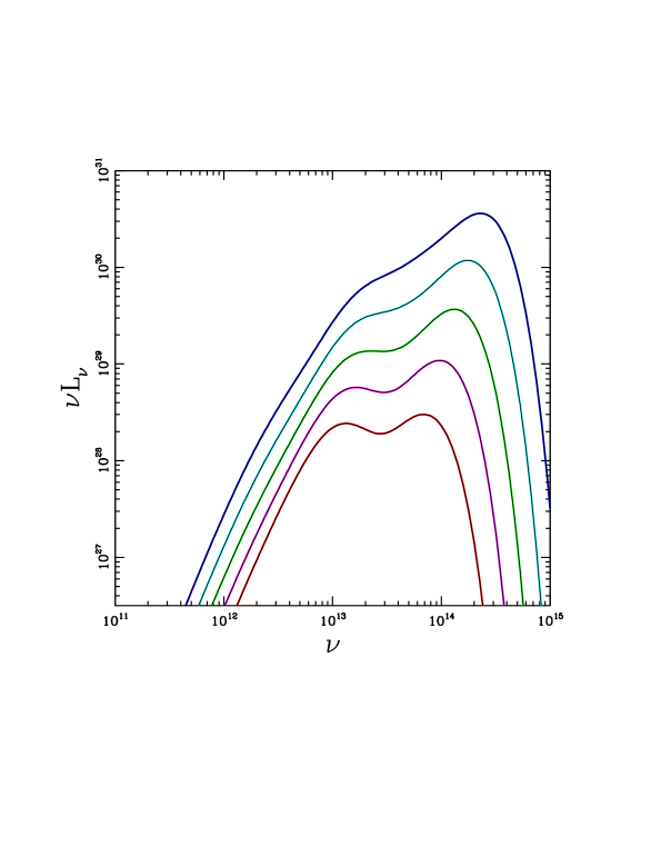
Figure 6: Emergent spectral energy distributions for a forming planet as a function of mass $M_{\rm p}$. The planet is assumed to have mass accretion rate ${\dot{M}}_{\rm p}$ = $1M_{J}$/Myr, radial location $a$ = 5 AU, and surface magnetic field strength $B_{\rm p}=500$ gauss. The curves show the spectral energy distributions for planet masses $M_{\rm p}$ = 0.1 $M_{J}$ (bottom, red), $10^{-1/2}M_{J}$ (magenta), $1M_{J}$ (middle, green), $10^{1/2}M_{J}$ (cyan), and $10M_{J}$ (top, blue). (Frequency $\nu$ is in Hertz and spectral energy $\nu L_{\nu}$ is in erg/s.)

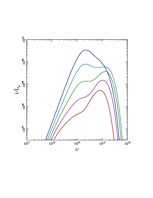
Figure 7: Emergent spectral energy distributions for a forming planet as a function of mass accretion rate ${\dot{M}}_{\rm p}$. The planet is assumed to have mass $M_{\rm p}=1M_{J}$, radial location $a$ = 5 AU, and surface magnetic field strength $B_{\rm p}=500$ gauss. The curves show the spectral energy distributions for mass accretion rates ${\dot{M}}_{\rm p}$ = 0.1 $M_{J}$/Myr (bottom, red), $10^{-1/2}M_{J}$/Myr (magenta), $1M_{J}$/Myr (middle, green), $10^{1/2}M_{J}$/Myr (cyan), and $10M_{J}$/Myr (top, blue). (Frequency $\nu$ is in Hertz and spectral energy $\nu L_{\nu}$ is in erg/s.)

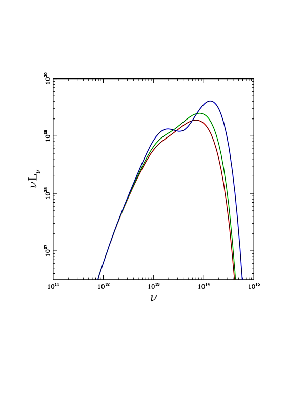
Figure 8: Emergent spectral energy distributions for a forming planet as a function of surface magnetic field strength $B_{\rm p}$ (which sets the location of the magnetic truncation radius $R_{X}$). The planet is assumed to have mass $M_{\rm p}=1M_{J}$, mass accretion rate ${\dot{M}}_{\rm p}=1M_{J}$/Myr, and radial location $a$ = 5 AU. The curves show the spectral energy distributions for surface magnetic field strength $B_{\rm p}=10$ gauss (bottom, red), 100 gauss (middle, green), and 1000 gauss (top, blue). For $B_{\rm p}$ = 10 gauss, the disk extends to the planetary surface. For $B_{\rm p}$ = 100 (1000) gauss, the disk is truncated at $R_{X}\approx 1.5(5.6)R_{\rm p}$. (Frequency $\nu$ is in Hertz and spectral energy $\nu L_{\nu}$ is in erg/s.)

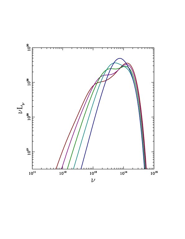
Figure 9: Emergent spectral energy distributions for a forming planet as a function of semimajor axis $a$ of the planetary orbit. The planet is assumed to have mass $M_{\rm p}=1M_{J}$, mass accretion rate ${\dot{M}}_{\rm p}=1M_{J}$/Myr, and surface magnetic field strength $B_{\rm p}$ = 350 gauss. The curves show the spectral energy distributions for semimajor axes $a$ = 10 AU (red), $10^{1/2}$ AU (magenta), 1 AU (green), $10^{-1/2}$ AU (cyan), and 0.1 AU (blue). (Frequency $\nu$ is in Hertz and spectral energy $\nu L_{\nu}$ is in erg/s.)

The emergent spectral energy distributions depend on four variables that define the system: the planet mass $M_{\rm p}$, the mass accretion rate ${\dot{M}}_{\rm p}$, the magnetic field strength $B_{\rm p}$ on the planetary surface, and the semimajor axis $a$ of the planetary orbit. With $(M_{\rm p},{\dot{M}}_{\rm p})$ specified, the field strength determines the magnetic truncation radius, which sets the inner edge of the disk. The semimajor axis determines the centrifugal radius, which sets the outer edge of the disk. We note that if a complete theoretical description of the planet formation process were available, then the dependence of the mass accretion rate and the magnetic field strength on planet mass and location could be calculated (see also Appendix E). In the absence of a complete theory, it is useful to see how the spectral energy distributions vary over the parameter space $(M_{\rm p},{\dot{M}}_{\rm p},B_{\rm p},a)$. For the sake of definiteness, we fix the planet radius so that $R_{\rm p}=10^{10}$ cm.

Figure 6 shows how the spectral energy distributions depend on the planet mass, which is varied over the range $M_{\rm p}$ = 0.1 – 10 $M_{J}$. For all of the models, the mass accretion rate is fixed at ${\dot{M}}_{\rm p}$ = $1M_{J}$/Myr, the semimajor axis $a$ = 5 AU, and surface magnetic field strength $B_{\rm p}=500$ gauss. Two trends are evident. First, as expected, the total luminosity of the planet/disk system increases with mass, so that the larger objects are brighter. Moreover, to leading order, $L\propto M_{\rm p}$. Second, the spectral energy distributions become bluer with increasing planet mass. For planets of higher mass, the planetary surface is hotter and the total optical depth through the infalling envelope is lower, so that a smaller fraction of the energy is emitted at longer wavelengths. These trends are consistent with previous numerical studies (Szulágyi et al., 2019).

The dependence of the spectral energy distributions on the mass accretion rate is shown in Figure 7, where ${\dot{M}}_{\rm p}$ = 0.1 – 10 $M_{J}$/Myr. In this case, the planet mass is fixed at $M_{\rm p}=1M_{J}$, the semimajor axis $a$ = 5 AU, and surface magnetic field strength $B_{\rm p}=500$ gauss. As before, two trends are present (compare with Figure 6). The total luminosity of the planet/disk system increases with the mass accretion rate, where the luminosity scales as $L\propto{\dot{M}}_{\rm p}$ to leading order. In this case, however, the the spectral energy distributions become redder with increasing luminosity (due to the larger mass accretion rate). The increase in ${\dot{M}}_{\rm p}$ corresponds to an increase in the column density, so that more of the central source radiation is absorbed by the infalling envelope and re-radiated into the infrared.

The effects of varying the magnetic field strength are shown in Figure 8. In this case, the $B_{\rm p}$ varies over the range 10 – 1000 gauss. The planet has mass $M_{\rm p}=1M_{J}$, accretion rate ${\dot{M}}_{\rm p}=1M_{J}$/Myr, and semimajor axis $a$ = 5 AU. For the smallest field value, $B_{\rm p}=10$ gauss, the magnetic truncation radius $R_{X}$ is smaller than the planetary radius, so that the disk extends all the way to the planetary surface. For stronger magnetic fields with $B_{\rm p}$ = 100 and 1000 gauss, the radius $R_{X}/R_{\rm p}$ = 1.5 and 5.6, respectively, and magnetic truncation becomes important. The larger values of $R_{X}$ lead to modest increases in the luminosity, due to less rotational energy being stored in the circumplanetary disk. Larger truncation radii $R_{X}$ also result in bluer planet/disk spectra, so that the extinction (for fixed column density) is greater. As a result, a double-humped form of the spectral energy distribution is produced for systems with large field strengths $B_{\rm p}$.

Figure 9 shows how the spectral energy distributions vary with the semimajor axis of the orbit of the forming planet. Here the planet mass $M_{\rm p}$ = 1 $M_{J}$, the accretion rate ${\dot{M}}_{\rm p}$ = 1 $M_{J}$/Myr, and the magnetic field strength is fixed at $B_{\rm p}=350$ gauss. Results are shown for semimajor axes in the range 0.1 – 10 AU. The spectral energy distributions become wider as the semimajor axis increases. The most important effect is that the radius of the circumplanetary disk scales as $R_{\rm d}\propto{R_{H}}\propto{a}$. For the lower end of the orbital range ($a=0.1$ AU), the disk radius becomes comparable to the magnetic truncation radius. In this regime, most of the radiation from the central source is emitted from a single surface temperature. Moreover, the column density is larger, so that more of the central source photons are absorbed and re-emitted by the envelope. The resulting spectral energy distribution thus approaches a blackbody form. For larger semimajor axes, the column density is smaller, and the spectral energy distributions are broader and bluer.

6 Conclusion

This paper has constructed an analytic approach to the late stages of accretion for the formation of gaseous giant planets. This work is applicable to the third stage of the formation process when the planet accretes the majority of its mass.

6.1 Summary of Results

Our main results can be summarized as follows:

We have developed an infall solution to describe the density and velocity fields of the material falling toward a forming giant planet. The flow enters into the sphere of influence of the planet near the Hill radius, and then smoothly approaches ballistic trajectories. In this approximation, the density distribution $\rho(r,\mu)$ (given by equations [5] and [12]) and the velocity field ${\vec{v}}(r,\mu)$ (given by equations [8 – 11]) are axisymmetric. The material with the highest specific angular momentum falls onto a circumplanetary disk with radius given by the centrifugal barrier ($R_{\rm d}=R_{C}=R_{H}/3$; equation [7]).

To gain insight into the nature of the region surrounding the forming planet, we have constructed the equivalent spherical density distribution (equations [13–15]). The total column density $N_{\rm col}$ (given by equation [17]) of the envelope plays an important role in determining the spectral energy distribution of the forming body. The envelope surrounding the planet is predicted to be marginally optically thick to the radiation emitted from the central planet/disk systems, but is predicted to be optically thin to radiation emitted by the envelope itself.

Most of the material falling toward the planet has too much specific angular momentum to reach the planetary surface. Instead, material falls onto a circumplanetary disk with radius $R_{C}$ determined by conservation of angular momentum (equation [7]) and an inner radius $R_{X}$ determined by magnetic truncation (equation [36]). Given the expected disk radius and mass accretion rate onto the disk, the time scale for viscous evolution is shorter than that for disk mass accumulation provided that the dimensionless parameter $\alpha\,\raise 1.29167pt\hbox{$>$}\kern-7.5pt\lower 3.01385pt\hbox{$\sim$}\,10^{-5}$. As result, the disk is expected to reach a steady state, with low mass compared to the central planet, and with a surface density distribution $\Sigma(r)$ given by equations (30) and (32).

Magnetic fields play an important role in determining the geometry of the inner disk and inner infall region. The balance between magnetic pressure and mass accretion rate through the disk defines the truncation radius $R_{X}$ (equation [36]), which specifies the inner disk edge. The field configuration also defines a capture radius $R_{\sigma}$ (equation [45]), which is determined by the balance between the ram pressure of infalling gas and the magnetic pressure at the point where the field lines are horizontal (see Figure 3).

The forming planet generates power from several contributions (see Section 5.1). The relevant luminosity sources include shocks from direct infall onto the planetary surface, accretion from the inner disk edge onto the planet, viscous accretion through the circumplanetary disk, as well as both shocks and mixing from material falling onto the disk surface. The planet generates additional internal power through gravitational contraction. The total luminosity is comparable to the benchmark power scale given by equation (47).

With the properties of the components specified, we have calculated radiative signatures of the planet forming process. The central planet and disk produce an intrinsic spectral energy distribution that corresponds to surface temperatures in the range $T=100-1000$ K (Figure 4). The infalling envelope attenuates the central source luminsity, which is re-radiated at longer wavelengths, primarily in the infrared. The resulting spectral energy distributions $\nu L_{\nu}$ are significantly broader than single-temperature blackbodies and show systematic variations with planet mass $M_{\rm p}$, accretion rate ${\dot{M}}_{\rm p}$, magnetic field strength $B_{\rm p}$, and semimajor axis $a$ (these trends are illustrated in Figures 5 – 9).

6.2 Star Formation versus Planet Formation

The infall-collapse-disk solutions constructed here for the formation of giant planets are analogous to those found earlier for the star formation problem (see the review of Shu et al. 1987). It is useful to outline the ways in which the formation processes are similar — and different — for the two cases. In both settings, angular momentum plays a key role in determining the geometry of the incoming material. Both star formation and planet formation produce nearly pressure-free collapse flow, with high angular momentum orbits that lead to the formation of a disk structure. Significantly, most of the mass initially falls onto the disk in both cases. The resulting dynamic range, as determined by the ratio of the disk radius to that of the central body, is much larger for star formation ($R_{C}/R_{\ast}\sim 10^{4}$) than for planet formation ($R_{C}/R_{\rm p}\sim 100$). Stars form much faster, with typical formation times of order 0.1 Myr, compared to 1 Myr for planets. With a longer formation times and smaller dynamic ranges, circumplanetary disks require much smaller viscosity to reach a steady-state where accretion through the disk keeps pace with infall onto the disk. Although the source of viscosity remains under study, modest values of the parameter $\alpha\sim 10^{-4}$ are sufficient to keep circumplanetary disks in steady-state (and such values are expected to be realized). Much larger viscosity levels are required for star-forming disks to reach steady-state. As a result, circumstellar disks are expected to experience gravitational instability during their early formative stages. In addition, the circumstellar disks are subject to episodic accretion, which produces FU Orionis outbursts. It remains to be seen if circumplanetary disks are subject to the same episodic behavior.

The dynamic range in temperature is also much larger for star formation, where the stellar surface has typical temperature $T_{\ast}\sim 6000$ K, and the outer part of the infall region has interstellar temperatures $T_{\rm ism}\sim 10-30$ K. For planet formation, the planetary surface temperature is significantly smaller $T_{\rm p}\sim$ $1000-1500$ K, and the temperature at the outer boundary is typically $T_{H}\sim 100$ K (for $a\sim 5$ AU). The temperature range for star formation (factor of $\sim 300$) is more than an order of magnitude greater than the range for planet formation (factor of $\sim 12$). Planets forming at smaller semimajor axes (e.g., $a\sim 0.1$ AU), have even smaller temperature ranges.

In both star and planet formation, the rate ${\dot{M}}$ at which the growing body gains mass is of fundamental importance. In the case of star formation, ${\dot{M}}_{\rm core}\approx v_{\rm s}^{3}/G$ is determined by the pre-collapse conditions in the background molecular cloud. This quantity determines the rate at which the entire star/disk system gains mass from its parental cloud. Dissipative processes within the circumstellar disk then determine the smaller rate ${\dot{M}}_{\ast{\rm d}}$ at which the disk accretes material onto the star. In the context of planet formation, the background circumstellar disk plays a role similar to the cloud in star formation. In the latter case, however, the semimajor axis of the planet determines the Hill radius, which in turn affects the accretion rate ${\dot{M}}_{\rm p}$ into the sphere of influence (where ${\dot{M}}_{\rm p}$ is a fraction of ${\dot{M}}_{\ast{\rm d}}$). Unlike stars, forming planets are thus subject to a systematic variation in background conditions, with corresponding variations in ${\dot{M}}$.

6.3 Discussion

To help organize our understanding of the late stages of the planet formation process, we can consider the ordering of the relevant length scales:

$$R_{\rm p}<R_{X}\sim R_{\sigma}\ll R_{C}\sim R_{\rm d}<R_{H}\sim H\ll a\,.$$ (72)

During the phase when the growing planet accretes most of its gas, the protoplanet thus develops a hierarchical structure. Most of the mass entering the sphere of influence from the background cirumstellar disk falls onto the circumplanetary disk, which is much larger than the planet itself. Magnetic fields lead to a truncation of the inner disk and provide a larger effective capture cross section at a scale of several planetary radii. The nominal disk radius is one third of the Hill radius, which is roughly comparable to the scale height of the circumstellar disk. For the formation of giant planets near or beyond the ice-line ($a\,\raise 1.29167pt\hbox{$>$}\kern-7.5pt\lower 3.01385pt\hbox{$\sim$}\,3$ AU), all of these scales are much smaller than the semimajor axis at the location of the planet. For hot Jupiters ($a\,\raise 1.29167pt\hbox{$<$}\kern-7.5pt\lower 3.01385pt\hbox{$\sim$}\,0.1$ AU), however, the length scales that define the outer disk ($R_{\rm d}$, $R_{C}$, $R_{H}$, $H$) become comparable to the magnetic radii ($R_{X}$, $R_{\sigma}$). This reordering of length scales implies that giant planet formation could proceed differently in the inner and outer (circumstellar) disk, with a boundary between the two regimes at roughly $a\sim 0.1$ AU.

The relevant time scales also have a well defined ordering,

$$t_{\rm disk}<t_{\rm orb}\ll t_{\rm vis}\ll t_{\rm form}\,\raise 1.29167pt\hbox{$<$}\kern-7.5pt\lower 3.01385pt\hbox{$\sim$}\,t_{\rm kh}\,.$$ (73)

The orbital time scale of the forming planet (around the star) is 9 times longer than the orbital time scale at the outer edge of the circumplanetary disk (around the planet), so that $t_{\rm orb}$ = $9t_{\rm disk}$. The viscous evolution time scale $t_{\rm vis}$ = $R_{C}^{2}/\nu$ of the circumplanetary disk is much longer than the orbit time, but much shorter than the formation time scale $t_{\rm form}$ = $M_{\rm p}/{\dot{M}}_{\rm p}$. As a result, the disk can evolve to a steady-state configuration (see equation [30]). The Kelvin-Helmholtz time scale $t_{\rm kh}$ sets the times scale for the evolution of the internal planetary structure, and is comparable to the formation time if the luminosity is determined by the scale $L_{0}$ from equation (47), but somewhat longer if we use only the internally generated luminosity to define $t_{\rm kh}$.

In general, the Hill radius $R_{H}$ provides the outer boundary for the planetary sphere of influence, including in this present work. Although this ansatz provides a good first approximation, the picture is more nuanced. Numerical simulations indicate that some of the material that initially flows into the Hill sphere promptly flows back out (e.g., Lambrechts et al. 2019). The treatment of this paper accounts for this loss by taking the mass infall rate ${\dot{M}}_{\rm p}$ to include only the material that initially stays within the Hill sphere and falls toward the planet. A related complication is that the Hill radius is only an approximation to the true boundary. Pressure and magnetic corrections lead to smaller values for the effective boundary between the planet and its background disk (Appendix C). A smaller boundary radius, in turn, leads to a smaller centrifugal barrier $R_{C}$, which sets the nominal radius of the circumplanetary disk (equations [5–7]). Two dimensional simulations find that the expected disk radius at $R_{C}=R_{H}/3$ provides a good approximation (Martin & Lubow, 2011), whereas three dimensional simulations find somewhat smaller values for $R_{C}$ (Fung et al., 2019). Three dimensional simulations (e.g., Lambrechts et al. 2019) show that infall takes place preferentially along the poles of the system. This confinement results in a smaller centrifugal radius ($R_{C}\to R_{C}[1-\mu_{b}^{2}]$) for a given planetary mass and a somewhat steeper surface density distribution. Finally, some of the material that initially falls onto the circumplanetary disk must eventually flow back out into the circumstellar disk. Viscous torques cause the circumplanetary disk to spread, so that most of the mass flows inward, but some mass flows outward to conserve angular momentum. As a result, some fraction of the disk material must diffuse beyond the outer boundary (given by the generalized Hill radius) and rejoin the background circumstellar disk. The analytic treatment developed in this paper is robust, in that it provides solutions for any value of the centrifugal radius. On the other hand, additional work is required to determine the expected values of $R_{C}$ to higher accuracy.

This analytic approach highlights how planet formation can vary with the location of the planetary orbit. For a given planetary mass, the physical size of the Hill radius and the circumplanetary disk radius grow with increasing semimajor axis $a$. Disk viscosity must play an increasingly important role for more distant planets. This trend has the effect of making planet formation (through the core accretion paradigm) more difficult with increasing $a$. This trend acts in addition to the previously discussed effect that the formation of planetary cores takes longer for larger orbits. In the opposite limit, for small orbits akin to those of hot Jupiters, accretion through circumplanetary disks is even more efficient. However, for $a\,\raise 1.29167pt\hbox{$<$}\kern-7.5pt\lower 3.01385pt\hbox{$\sim$}\,0.1$ AU, the expected magnetic truncation radius becomes smaller than the disk radius, and infall onto the entire planet/disk system can be suppressed.

This paper also provides an analytic description of the radiative signature of forming gas giants. Observations of dust emission from circumplanetary disks (which are embedded within circumstellar disks) have just become technologically possible (Benisty et al., 2021) and more such detections are expected. Current observations of circumplanetary disks are roughly consistent with theoretical expectations — including those of this paper. As future observations further elucidate the properties of forming planets, the analytic treatment of this paper can be readily adopted and generalized to provide theoretical descriptions of the formation process.

Acknowledgments: We are grateful to A. Adams, M. Meyer, and D. Stevenson for useful discussions. We thank an anonymous referee for many helpful comments. This work was supported by the University of Michigan, Caltech, the Leinweber Center for Theoretical Physics, and by the David the Lucile Packard Foundation.

Appendix A Approximation Control

The main text presents a working analytic model for the infall of material onto a forming planet and its circumplanetary disk, along with solutions for the evolution of the disk. With the model in place, this Appendix outlines the requirements for the solutions to be self consistent. More specifically, we estimate the magnitude of the errors introduced in making the approximations necessary for an analytic treatment.

The infall collapse solution is constructed using a constant mass $M_{\rm p}$ for the planet. Consistency requires that the time scale for the planet mass to change must be much longer than the time required for parcels of gas to fall inward. The evolution time for the mass of the planet is expected to be $t_{\rm acc}=M_{\rm p}/{\dot{M}}_{\rm p}\sim$ 1 Myr. For comparison, the infall time from the outer boundary is given by

$$t_{\rm in}\sim\left({GM_{\rm p}\over R_{H}^{3}}\right)^{-1/2}=\left({3GM_{\ast}\over a^{3}}\right)^{-1/2}\approx 1\,{\rm yr}\,\left({M_{\ast}\over 1M_{\odot}}\right)^{-1/2}\left({a\over 5\,{\rm AU}}\right)^{3/2}\,.$$ (A1)

We thus find $t_{\rm in}\ll t_{\rm acc}$ as required. Planets can also change their radial locations (migrate) during the time when they acquire mass. The typical migration time scales are of order $\sim 1$ Myr, so that the infall time scale is much shorter, and the analytic solutions of this work are applicable.

Another assumption is that the infalling gas follows ballistic trajectories, which require that the pressure forces are much smaller than the gravitational forces. At the outer boundary, given by the Hill radius, this requirement can be written in the approximate form

$${GM_{\rm p}\over R_{H}^{2}}\gg{1\over\rho}{dP\over dr}\approx\Omega^{2}R_{H}G(\theta)\,,$$ (A2)

where the second equality follows from the assumption that the circumstellar disk is locally in hydrostatic equilibrium. The geometrical factor $G(\theta)$ is unity in the $\hat{z}$ direction, which we take to be along the pole of the planet, whereas $G\sim H/a$ along the equatorial directions. Using $\Omega^{2}$ = $GM_{\ast}/a^{3}$ and the definition of the Hill radius, we find that the left-hand side of the equation is larger than the right-hand side by a factor of $3$ for polar directions and a factor of $\sim 30$ for equatorial directions. Alternately, we can compare the depth of the potential well $GM_{\rm p}/R_{H}$ with the local sound speed $v_{s}^{2}$. For a Jovian planet forming at $a=5$ AU, the gravitational potential well at $R_{H}$ corresponds to a speed $\sim 1.6$ km/s. The sound speed is given by $v_{\rm s}\approx 0.72$ km/s ($T$/130K)^1/2, so the pressure is subdominant by a factor of $\sim 5$ for the values used here. Moreover, pressure forces will become less important as the flow moves inward, provided that the equation of state is not too stiff. Specifically, studies of collapse solutions for star formation show that if the dynamic equation of state has the polytropic form $P\propto\rho^{\gamma}$, the requirement $\gamma<5/3$ allows for trajectories to remain ballistic (Fatuzzo et al. 2004; see also McKee & Holliman 1999). On the other hand, a sufficiently stiff equation of state (corresponding to inefficient cooling and hence large $\gamma$) can result in non-negligible pressure terms. Numerical simulations (Fung et al., 2019) show similar trends, where an isothermal equation of state leads to the formation of rotationally supported disks, but adiabatic simulations result in extended structures.

The orbit equation that describes infalling trajectories was derived for the gravitational potential of a point mass. However, the extended structure of the circumplanetary disk will cause orbits to precess relative to this approximation. The first non-zero correction to the potential corresponds to the quadrupole term, which decreases rapidly with radial distance. In addition, the disk mass is expected to be small, with $M_{\rm d}/M_{\rm p}\sim$ ${\cal R}\sim 0.01$.

The infalling trajectories were taken to be zero energy orbits. Since the incoming gas enters the sphere of influence at the Hill sphere, the total speed of the gas must be given by $v^{2}=2GM_{\rm p}/R_{H}$ for consistency. Here we assume that the specific angular momentum is given by $j_{\infty}=\Omega R_{H}^{2}$, so that one component of the velocity is $\Omega R_{H}$. Since $(\Omega R_{H})^{2}=GM_{\rm p}/3R_{H}$, we are implicitly assuming that the other incoming velocity components add up to $v_{\perp}^{2}=5GM_{\rm p}/3R_{H}$. If the actual (non-rotational) velocity components were zero, then the zero-energy approximation corresponds to a relative error in energy of $5r/6R_{H}$. This energy inconsistency is only $\sim 0.16\%$ for orbits that land on the planetary surface, but grows to $\sim 28\%$ for orbits that fall to the outer edge of the disk (see also Mendoza et al. 2009 for further generalizations of the infall trajectories).

The initial conditions for infall, and hence the resulting solutions, are assumed to be azimuthally symmetric. Numerical simulations of the planet formation process indicate that the incoming flow can be concentrated into streamers, thus breaking the symmetry. However, this complication has only a modest affect on the properties of the circumplanetary disk and the forming planet. The incoming material primarily falls onto the disk, where it enters a nearly Keplerian orbit around the planet. The orbital time scale at the outer disk edge is much shorter ($\sim 1$ year) than the time scale on which the planet gains mass ($\sim 1$ Myr). As a result, differential rotation rapidly spreads material over the orbit so that the disk becomes azimuthally symmetric. On the other hand, for purposes of calculating the spectral signatures (Section 5), we carry out the radiative transfer for a fully spherical envelope. These spherical solutions would be modified with non-axisymmetric infalling envelopes. The results are model dependent, however, and this generalization is left for future work.

The treatement has ignored magnetic field effects in determining the properties of the infalling envelope. In order for magnetic fields to influence infall onto the disk to a significant degree, the magnetic pressure must compete with the ram pressure of the infall at the outer disk edge. This consideration implies the consistency condition

$${B_{C}^{2}\over 8\pi}\,\raise 1.29167pt\hbox{$<$}\kern-7.5pt\lower 3.01385pt\hbox{$\sim$}\,\rho v^{2}={{\dot{M}}_{\rm p}v_{C}\over 4\pi R_{C}^{2}}\,,$$ (A3)

where the subscripts indicate that the quantities are evaluated at the disk edge. The magnetic field strength $B_{C}$ at the edge is less than or equal to the value indicated by flux-freezing, i.e., $B_{C}\leq B_{0}$ $(R_{H}^{2}/R_{C}^{2})=9B_{0}$, where $B_{0}$ is the magnetic field strength of the circumstellar disk material evaluated outside the Hill sphere (note that $B_{0}$ is expected to be a function of semimajor axis $a$). We obtain a sufficient condition on $B_{0}$ by combining the above expressions to obtain

$$B_{0}\,\raise 1.29167pt\hbox{$<$}\kern-7.5pt\lower 3.01385pt\hbox{$\sim$}\,\sqrt{2\over 9}\left[{GM_{\rm p}{\dot{M}}_{\rm p}^{2}\over R_{C}^{5}}\right]^{1/4}\approx 36\,{\rm mG}\,\left({M_{\rm p}\over M_{J}}\right)^{-1/6}\left({{\dot{M}}_{\rm p}\over 1M_{J}/{\rm Myr}}\right)^{1/2}\left({a\over 5\,{\rm AU}}\right)^{-5/4}\,.$$ (A4)

Since most estimates for disk magnetic field strengths are below this value, the disk can form as described in the main text. Note that if flux-freezing holds down to smaller radii, $r\ll R_{C}$, then the inner regions could be magnetically affected for sufficiently large values of $B_{0}$. In this case, magnetic fields could cause the infalling parcels of gas to fall to larger radii within the disk, thereby leading to smaller shock luminosity from the disk surface. As long as the disk viscosity is large enough, however, the disk would accrete as before and deliver the same amount of material to the planet. Moreover, if the volume density of the gas exceeds a threshold of $n\sim 10^{11}$ cm^-3, coupling between the magnetic field and the fluid is compromised, and the magnetic flux can be dynamically redistributed (Nishi et al., 1991; Desch & Mouschovias, 2001).

Another consideration for magnetic field effects is the time required for the resistivity $\eta$ to change the field structure. The resistivity acts as a diffusion constant, so that the time scale for field evolution over a length scale $\ell$ is given approximately by $t\sim\ell^{2}/\eta$. If we require that the resistivity is large enough so that this time scale is less than the free-fall time, the constraint on $\eta$ at the Hill radius $R_{H}$ takes the form

$$\eta\,\raise 1.29167pt\hbox{$>$}\kern-7.5pt\lower 3.01385pt\hbox{$\sim$}\,\sqrt{GM_{\rm p}a}\left({M_{\rm p}\over 3M_{\ast}}\right)^{1/6}=8.3\times 10^{17}{\rm cm}^{2}{\rm s}^{-1}\left({a\over 5{\rm AU}}\right)^{1/2}\left({M_{\rm p}\over m_{J}}\right)^{2/3}\,.$$ (A5)

Estimates for the appropriate resistivity in circumstellar disks, which provide the background environment for the collapse flow, vary widely. Estimates for the resistivity include the range $\eta=10^{16}-10^{19}$ cm² s^-1 (Stepinski, 1992), $\eta\approx 10^{16}$ cm² s^-1 (Wardle & Ng, 1999), $\eta\approx 10^{19}$ cm² s^-1 (Desch & Mouschovias, 2001), and $\eta\approx 10^{20}$ cm² s^-1 (Shu et al., 2006). In addition to the electrical resistivity, ambipolar diffusion can provide a substantial contribution $\eta_{\scriptstyle AD}$ $\sim B^{2}/(4\pi\gamma\rho_{i}\rho_{n})$, where $\gamma$ is the ion-neutral drag coefficient and $\rho_{i}$ and $\rho_{n}$ are the ion and neutral densities (see also Nakano et al. 2002). In summary, most estimates indicate that $\eta$ is large enough for magnetic fields to diffuse outward fast enough for the flow to remain in the kinematic regime, although further work must be carried out.

Appendix B Planetary Magnetic Field Strength

Since the magnetic field can play an important role in accretion of material onto a forming planet, we need to estimate the expected field strength. One now-standard scaling law assumes that the field strength is proportional to the energy generation rate due to buoyancy forces (e.g., Christensen et al. 2009; Yadav & Thorngren 2017). This law can be written in the form

$${B^{2}\over\rho}\sim\ell^{2/3}{\cal P}^{2/3}\,,$$ (B1)

where ${\cal P}$ is the energy production rate per unit mass and $\ell$ is a length scale associated with the size of a convective cell. We expect the length $\ell$ to be a fraction of the planetary radius

$$\ell=f_{\ell}R_{\rm p}\,.$$ (B2)

In this expression, $B$ is the field strength in the dynamo region. The surface field will be a fraction of this value so that

$$B_{\rm p}=f_{B}B\,.$$ (B3)

Finally, we expect the power transported through the planetary interior to be a fraction $f_{P}$ of the total power generated by the object, where the latter is dominated by accretion. As a result, we can write

$${\cal P}=f_{P}{G{\dot{M}}_{\rm p}\over R_{\rm p}}\,.$$ (B4)

Significantly, we expect the three factors $(f_{\ell},f_{B},f_{P})$ to all be less than unity. The surface field then takes the form

$$B_{\rm p}^{2}=f_{T}{3M_{\rm p}f_{\rho}\over 4\pi R_{\rm p}^{3}}\left(G{\dot{M}}_{\rm p}\right)^{2/3}\qquad{\rm where}\qquad f_{T}\equiv f_{B}^{2}f_{\ell}^{2/3}f_{P}^{2/3}\,.$$ (B5)

The factor $f_{\rho}$ takes into account the difference between the mean density of the planet and that of the convective cells; the second equality collects the other dimensionless factors into a single quantity $f_{T}<1$. Inserting typical values, we find the field strength estimate

$$B_{\rm p}\approx 1600\,{\rm gauss}\,\,\,f_{T}^{1/2}\left({\rho\over 1\,{\rm g}\,{\rm cm}^{-3}}\right)^{1/2}\left({{\dot{M}}_{\rm p}\over 1\,M_{J}\,{\rm Myr}^{-1}}\right)^{1/3}\,.$$ (B6)

The factor $f_{T}$ can be much smaller than unity, so that the numerical value provides an appoximate upper limit to the expected field strength. Nonetheless, substantial magnetic fields can be produced within forming planets if sufficient accretion energy is converted into convective motions. For example, if we take $f_{B}=1/2=f_{\ell}$ and $f_{P}=1/10$, then $B_{\rm p}\approx 300$ gauss.

Appendix C Corrections to the Hill Radius

In the treatment of this paper, the Hill radius $R_{H}$ marks the boundary between the circumstellar disk and the region where the gravitational influence of the planet dominates. The Hill radius sets the centrifugal radius for the collapse flow (where $R_{C}=R_{H}/3$) and thus determines the disk radius ($R_{\rm d}=R_{C}$). Given that this boundary plays an important role in the planet formation problem, this Appendix considers possible corrections.

The effects of pressure can be accounted for in the derivation of the Hill radius. The net effect of including pressure is to reduce the effective mass of the planet for purposes of defining the extent of its influence. The pressure-corrected Hill radius can thus be written in the form

$$R_{H*}=a\left({f_{\rm pc}M_{\rm p}\over 3M_{\ast}}\right)^{1/3}\,,$$ (C1)

where $f_{\rm pc}$ is a dimensionless factor less than unity. Using this result in the definition of the centrifugal radius (7), we find the pressure-corrected form

$$R_{C*}={f_{\rm pc}\over 3}R_{H*}=f_{\rm pc}^{4/3}{R_{H}\over 3}\,.$$ (C2)

We expect $f_{\rm pc}\sim 2/3$ (see Appendix A) so that the correction factor is $f_{\rm pc}^{4/3}\sim 0.58$ and the disk radius $R_{\rm d}$ = $R_{C*}\sim R_{H}/5$ (where $R_{H}$ is the usual, uncorrected, Hill radius).

With this correction, the mass scale $M_{0}$ that defines when the centrifugal radius exceeds the planetary radius becomes

$$M_{0}=\left({3\over f_{\rm pc}}\right)^{4}\left({R_{\rm p}\over a}\right)^{3}\,.$$ (C3)

Equation (44) gives the planet mass $M_{\rm p}$ for a given total mass $M$ that has fallen into the Hill sphere. The planet mass $M_{\rm p}\propto M_{0}^{1/3}\propto f_{\rm pc}^{-4/3}$. As a result, larger pressure suppression leads to a smaller centrifugal barrier and more mass being directly accreted onto the planet.

The discussion thus far uses the Hill radius as the boundary between the forming planet and the background circumstellar disk. An alternate choice is to the use the sphere of influence from astrodynamics (e.g., Danby 2003). The standard expression for this boundary has the form

$$R_{S}={a\over 2^{1/5}}\left({M_{\rm p}\over M_{\ast}}\right)^{2/5}\,.$$ (C4)

For planets with Jovian mass, $M_{\rm p}=1M_{J}$, we find that $R_{S}\approx 0.79R_{H}$, so the difference is modest. However, the centrifugal barrier $R_{C}\propto R_{S}^{4}$, so that the correction can be substantial. In addition, the scaling with mass is somewhat different. Moreover, using the sphere of influence $R_{S}$ allows for a staightforward way to include pressure forces into the definition of the boundary. As outlined in Appendix A, gravitational forces due to the planet are (at least) 3 times greater than the pressure forces at the Hill sphere. This finding implies that the gravitational acceleration used in the derivation of the sphere of influence is reduced by a factor of $f\sim 2/3$. The pressure-corrected sphere of influence can thus be written in the form

$$R_{S}={a\over 2^{1/5}}\left({fM_{\rm p}\over M_{\ast}}\right)^{2/5}\,.$$ (C5)

This radius thus defines the specific angular momentum at the starting point for collapse. The corresponding centrifugal radius becomes

$$R_{C}=a\left({f^{2}\over 2}\right)^{4/5}\left({M_{\rm p}\over M_{\ast}}\right)^{3/5}\,.$$ (C6)

Note that both the coefficient and the scaling with mass are different than in the previous case (using the Hill radius).

Appendix D Disk Solution Beyond the Centrifugal Barrier

The steady-state solution found in the main text applies over the radial range $R_{\rm p}\leq{r}\leq R_{C}$. However, the disk will spread beyond the centrifugal barrier. In this regime, the steady-state solution for the surface density is given by

$$r^{1/2}{d\over dr}\left(r^{1/2}\nu\Sigma\right)=constant\,,$$ (D1)

which has a solution of the form

$$\nu\Sigma=C_{0}+C_{1}u^{-1/2}\,,$$ (D2)

where $u=r/R_{C}$ (and $u>1$ in this regime). The constants $C_{0}$ and $C_{1}$ can be specified by requiring continuity of both $\Sigma(u)$ and its spatial derivative across the boundary $u=1$ ($r=R_{C}$). These matching conditions produce the constraints

$$C_{0}+C_{1}={{\dot{M}}_{\rm p}\over 12}\qquad{\rm and}\qquad{C_{1}\over C_{0}+C_{1}}=1\,.$$ (D3)

The constants thus have values $C_{0}=0$ and $C_{1}={\dot{M}}_{\rm p}/12$. The disk surface density thus decreases more rapidly (by a factor of $r^{-1/2}$) beyond the centrifugual barrier, which defines the nomimal disk radius.

Notice also that the disk must spread outward in order to satisfy conservation of angular momentum globally. Before collapse, the total angular momentum within the Hill sphere for a planetary mass $M_{\rm p}$ is given by

$$J={2\over 5}M_{\rm p}R_{H}^{2}\Omega\,.$$ (D4)

After collapse, the planet and its disk must account for this amount of angular momentum. If we consider the angular momentum of the spinning planet to be negligible in comparison, then some mass increment $\Delta{M}$ must orbit a large distance $R$ in order to carry the angular momentum $J$. Setting $R=R_{H}$ and solving for the required mass increment, we find

$${\Delta M\over M_{\rm p}}={2\over 5\sqrt{3}}\approx 0.23\,.$$ (D5)

In other words, roughly one quarter of the mass must spread out to the Hill sphere so that the material forming the planet can lose enough angular momentum to reach small radial distances. This results holds in the absence of any redistribution of angular momentum before the collapse. The action of pressure and magnetic fields can reduce the effective centrifugal barrier (see Appendix C), leading to a lower estimate for the mass increment $\Delta M$.

Appendix E Evolution

The analytic model developed in this paper provides solutions for the properties of the planet/disk/envelope system for any combination of the input parameters. These output properties include the envelope density distribution $\rho(r,\mu)$, velocity field ${\vec{v}}(r,\mu)$, column density $N_{\rm col}$, disk radius $R_{\rm d}=R_{C}$, magnetic truncation radius $R_{X}$, magnetic capture radius $R_{\sigma}$, and the resulting spectral energy distributions $\nu L_{\nu}(\nu)$. The required input parameters include the planet mass $M_{\rm p}$, radius $R_{\rm p}$, accretion rate ${\dot{M}}_{\rm p}$, magnetic field strength $B_{\rm p}$, and the semimajor axis $a$ of the forming object. In this treatment, we consider the planet radius as a slowly varying parameter and fix its value ($R_{\rm p}\sim 10^{10}$ cm). However, one could consider the case where cooling is inefficient and the planetary radius is much larger. In the present context, we are left with the input variables $(M_{\rm p},{\dot{M}}_{\rm p},B_{\rm p},a)$ that specify the system.

In a complete theory, which is not yet available, the parameters $(M_{\rm p},{\dot{M}}_{\rm p},B_{\rm p},a)$ are a function of time. For example, one expects $M_{\rm p}\sim\int{\dot{M}}_{\rm p}dt$. Working within this analytic model, we can consider evolutionary scenarios in which the parameters are interdependent. This dependence reduces the number of parameters and allows for the construction of an evolutionary sequence.

As one example, the mass accretion rate is likely to depend on planet mass. Many authors have suggested that the mass accretion rate ${\dot{M}}_{\rm p}$ is a power-law function of the Hill radius so that

$${\dot{M}}_{\rm p}={\dot{M}}_{0}\left({R_{H}\over R_{0}}\right)^{p}={\dot{M}}_{0}\left({M_{\rm p}\over M_{0}}\right)^{p/3}\,,$$ (E1)

where $p=4$ is the most common choice. If we specify the mass scale $M_{0}=M_{J}$, then the relevant input parameter is the accretion scale ${\dot{M}}_{0}$. We expect ${\dot{M}}_{0}\sim 1M_{J}$/Myr so that giant planets can gain enough mass during the lifetimes of circumstellar disks (where $\tau\sim 3$ Myr; Hernández et al. 2007). In addition, one can show that basic form of the planetary mass function can be reproduced under the assumption that accretion ends due to the removal of gas from the circumstellar disk (Adams et al., 2021). In any case, if the mass accretion rate is determined by equation (E1), the number of input variables is reduced.

The magnetic field strength $B_{\rm p}$ depends on both the planet mass and the accretion rate. Although dynamo theory remains incomplete, we can consider approximate scaling laws (Appendix B). Using equation (E1) to specify the mass dependence of the accretion rate, in conjunction with equation (B5), the field strength scales as $B_{\rm p}\propto M_{\rm p}^{17/18}$. As a result, the magnetic truncation radius from equation (36) scales with mass according to $R_{X}\propto M_{\rm p}^{1/63}$. The magnetic truncation radius is thus nearly constant as the planet mass grows (in this scenario).

For a given formation location, as set by the semimajor axis $a$, the above considerations define an evolutionary scenario. For a given time, equivalently planet mass, the accretion rate is specified by equation (E1) and the magnetic truncation radius is approximately constant.

Finally, we note that this formalism can also be used to consider migration scenarios. If the planet moves inward according to

$${{\dot{a}}\over a}=-{1\over\tau_{a}}\,,$$ (E2)

then $(da/dM)/a=-1/({\dot{M}}_{\rm p}\tau_{a})$. One can thus determine the planet location (semimajor axis $a$) as a function of planet mass. As long as the time scale for migration $a/{\dot{a}}$ sufficiently long (compared to the time required for the infall solution to adjust), the results of this paper continue to hold.

References

- Abramowitz & Stegun (1972) Abramowitz, M., & Stegun, I. A. 1972, Handbook of Mathematical Functions (New York: Dover)
- Adams et al. (2021) Adams, F. C., Meyer, M. M., & Adams, A. D. 2021, ApJ, 909, 1
- Adams & Shu (1985) Adams, F. C., & Shu, F. H. 1985, ApJ, 296, 655
- Adams & Shu (1986) Adams, F. C., & Shu, F. H. 1986, ApJ, 308, 836
- Batygin (2018) Batygin, K. 2018, AJ, 155, 178
- Batygin & Morbidelli (2020) Batygin, K., & Morbidelli, A. 2020, ApJ, 894, 143
- Benisty et al. (2021) Benisty M., Bae, J., Facchini, S., et al., 2021, ApJ, 916, L2
- Benz et al. (2014) Benz, W., Ida, S., Alibert, Y., Lin, D., & Mordasini, C. 2014, in Protostars and Planets VI, ed. H. Beuther et al. (Tucson, AZ: Univ. Arizona Press), 691
- Blandford & Payne (1982) Blandford, R. D., & Payne, D. G. 1982, MNRAS, 199, 883
- Boccaletti et al. (2020) Boccaletti A., Di Folco, E., Pantin, E., Dutrey, A., Guilloteau, S. Tang, Y. W., Piétu, V., Habart, E., Milli, J., Beck, T. L., & Maire, A.-L. 2020, A&A, 637, L5
- Cassen & Moosman (1981) Cassen, P., & Moosman, A. 1981, Icarus, 48, 353
- Cassen & Summers (1981) Cassen, P., & Summers, A. 1983, Icarus, 53, 26
- Chevalier (1983) Chevalier, R. 1983, ApJ, 268, 753
- Choksi & Chiang (2021) Choksi, N., & Chiang, E. 2021, arXiv:2110.00029
- Cridland (2018) Cridland, A. J. 2018, A&A, 619, 165
- Christensen et al. (2009) Christensen, U. R., Holzwarth, V., & Reiners A. 2009, Nature, 457, 167
- Danby (2003) Danby, J.M.A. 2003, Fundamentals of Celestial Mechanics (2nd edition; Richmond, VA: Willmann-Bell)
- Desch & Mouschovias (2001) Desch, S. J., & Mouschovias, T. 2001, ApJ, 550, 314
- Draine & Lee (1984) Draine, B. T., & Lee, H. M. 1984, ApJ, 285, 89
- Fatuzzo et al. (2004) Fatuzzo, M., Adams, F. C., & Myers, P. C. 2004, ApJ, 615, 813
- Fung et al. (2019) Fung, J., Zhu, Z., & Chiang E. 2019, ApJ, 887, 152
- Ghosh & Lamb (1978) Ghosh, P., & Lamb, F. K. 1978, ApJ, 223, L83
- Haisch et al. (2001) Haisch, K.E., Lada, E.A., & Lada, C.J. 2001, ApJ, 553, L153
- Hartmann (2009) Hartmann, L. W. 2009, Accretion Processes in Star Formation (Cambridge: Cambridge Univ. Press)
- Hashimoto et al. (2020) Hashimoto, J., Aoyama, Y., Konishi, M., et al. 2020, AJ, 159, 222
- Hernández et al. (2007) Hernández, J., Hartmann, L., Megeath, M. et al. 2007, ApJ, 662, 1067
- Hubickyj et al. (2005) Hubickyj, O., Bodenheimer, P., & Lissauer, J. J. 2005, Icarus, 179, 415
- Huang et al. (2018) Huang, J., Andrews, S. M., Dullemond, C. P., et al. 2018, ApJ, 869, L42
- Lambrechts & Lega (2017) Lambrechts, M., & Lega, E. 2017, A&A, 606, 146
- Lambrechts et al. (2019) Lambrechts, M., Lega, E., Nelson, R. P., Crida, A., & Morbidelli, A. 2019, A&A, 630, 82
- Lee (2019) Lee, E. J. 2019, ApJ, 878, 36
- Lissauer et al. (2009) Lissauer, J. J., Hubickyj, O., D’Angelo, G., & Bodenheimer, P. 2009, Icarus, 199, 338
- Machida et al. (2008) Machida, M. N., Kokubo, E., Inutsuka, S., & Matsumoto, T. 2008, ApJ, 685, 1220
- Malik et al. (2015) Malik, M., Meru, F., Mayer, L., & Meyer, M. 2015, ApJ, 802, 56
- Marley et al. (2007) Marley, M. S., Fortney, J. J., Hubickyj, O., Bodenheimer, P., & Lissauer, J. J. 2007, ApJ, 655, 541
- Martin & Lubow (2011) Martin R. G., & Lubow S. H. 2011, MNRAS, 413, 1447
- McKee & Holliman (1999) McKee, C. F., & Holliman, J. H., II 1999, ApJ, 522, 313
- Mendoza et al. (2009) Mendoza, S., Tejeda, E., & Nage, E. 2009, MNRAS, 393, 579
- Mohanty & Shu (2008) Mohanty, S., & Shu, F. H. 2008, ApJ, 687, 1323
- Nakano et al. (2002) Nakano, T., Nishi, R., & Umebayashi, T. 2002, ApJ, 573, 199
- Nishi et al. (1991) Nishi, R., Nakano, T., & Umebayashi, T. 1991, ApJ, 368, 181
- Quillen & Trilling (1998) Quillen, A. C., & Trilling, D. E. 1998, ApJ, 508, 707
- Perez-Becker & Chiang (2011) Perez-Becker, D., & Chiang, E. 2011, ApJ, 735, 8
- Pollack et al. (1996) Pollack, J. B., Hubickyj, O., Bodenheimer, P., Lissauer, J. J., Podolak, M., & Greenzweig, Y. 1996, Icarus, 124, 62
- Semenov et al. (2003) Semenov, D., Henning, Th., Helling, Ch., Ilgner, M., & Sedlmayr, E. 2003, A&A, 410, 611
- Shu et al. (1987) Shu, F. H., Adams, F. C., & Lizano, S. 1987, ARA&A, 25, 23
- Shu et al. (2006) Shu, F. H., Galli, D., Lizano, S., & Cai, M. 2006, ApJ, 647, 382
- Stepinski (1992) Stepinski, T. F. 1992, Icarus, 97, 130
- Szulágyi et al. (2016) Szulágyi, J. Masset, F., Lega, E., Crida, A., Morbidelli, A., & Guillot, T. 2016, MNRAS, 460, 285
- Szulágyi (2017) Szulágyi, J. 2017, ApJ, 842, 103
- Szulágyi & Mordasini (2017) Szulágyi, J., & Mordasini, C. 2017, MNRAS, 465, 64
- Szulágyi et al. (2019) Szulágyi, J. Dullemond, C. P., Pohl, A., & Quanz, S. P. 2019, MNRAS, 487, 1248
- Tanigawa et al. (2012) Tanigawa, T., Ohtsuku, K., & Machida, M. N. 2012, ApJ, 747, 47
- Tanigawa & Tanaka (2016) Tanigawa, T., & Tanaka, H. 2016, ApJ, 823, 48
- Tanigawa & Watanabe (2002) Tanigawa, T., & Watanabe, S.-I. 2002, ApJ, 580, 506
- Terebey et al. (1984) Terebey, S., Shu, F. H., & Cassen, P. 1984, ApJ, 286, 529
- Thanathibodee et al. (2019) Thanathibodee, T., Calvet, N., Bae, J., Muzerolle, J., & Hernández, R. F. 2019, ApJ, 885, 94
- Ulrich (1976) Ulrich, R. K. 1976, ApJ, 210, 377
- Wardle & Ng (1999) Wardle, M., & Ng, C. 1999, MNRAS, 303, 239
- Yadav & Thorngren (2017) Yadav, R. K., & Thorngren, D. P. 2017, ApJ Letters, 849, L12
- Zhang et al. (2021) Zhang, K., Booth, A. S., Law, C. J. et al. 2021, ApJS, 257, 5
- Zhu (2015) Zhu, Z. 2015, ApJ, 799, 16
- Zhu et al. (2018) Zhu, Z., Andrews, S. M., & Isella, A. 2018, MNRAS, 479, 1850
- Zhu et al. (2011) Zhu, Z., Nelson, R. P., Hartmann, L., Espaillat, C., & Calvet, N., 2011, ApJ, 729, 47