Renormalized Sparse Neural Network Pruning

Abstract

Large neural networks are heavily over-parameterized. This is done because it improves training to optimality. However once the network is trained, this means many parameters can be zeroed, or pruned, leaving an equivalent sparse neural network. We propose renormalizing sparse neural networks in order to improve accuracy. We prove that our method’s error converges to zero as network parameters cluster or concentrate. We prove that without renormalizing, the error does not converge to zero in general. We experiment with our method on real world datasets MNIST, Fashion MNIST, and CIFAR-10 and confirm a large improvement in accuracy with renormalization versus standard pruning.

1 Introduction

Sparse neural networks are being studied more as neural networks get deployed to edge devices and internet-of-things devices Mao et al. [2017]. Sparse neural networks have many parameters set to zero to decrease both computation and memory requirements. The simplest and most common pruning method is to train a neural network and then set the smallest weights, in absolute value, to zero. This ‘one-shot’ method can sparsify over 90% of the network’s parameters with less than 1% accuracy loss Liu et al. [2015], Mao et al. [2017]. We have reproduced some of these results. In Section 2, we describe our method and give the relevant theorems. In Section 3, we give experimental results and discuss the experimental setup. In Section 4, we conclude.

2 Method and Theoretic Results

We consider the simplest pruning method that sets a subset of the network parameters to zero and does not do any further training or optimization, also known as ‘one-shot’. Also we consider standard training and no special sparsity inducing training such as Louizos et al. [2017], Zimmer et al. [2022], Grigas et al. [2019], Miao et al. [2021]. We propose Renormalized Pruning which is a rescaling of the sparsified parameters, see Algo. 1.

We prove that the Renormalized Pruning approximation error is bounded and the error is consistent in terms of concentrations of neural network parameters. Renormalized Pruning is accurate up to two terms of the variance or range of neural network parameters, $a_{i}$, and features (or embeddings), $\phi_{i}$, times the amount of pruning done, $M$. The error converges to zero at a linear rate. Then we show that standard pruning does not converge in general, in this scenario. Note that the $M$-sparse neural network, $\Phi_{M}$, need not remove the smallest $a_{i}$. This is very relevant in the very high sparsity regime, >90% sparsity. At a neural network’s initial randomization, neural networks produce random features for a given input and then linearly combine them in the final layer to make a prediction. We can write this approximation of function $f$ as $f(x)\approx\sum_{i}a_{i}\phi_{i}(x)$ where $f$ is the function to approximate or predict, $a_{i}\in{\mathbb{R}}$, and function $\phi_{i}$ is randomly sampled from a distribution, for each $i$. Random features, also known as random embeddings, are good approximators when $a_{i}$ is chosen optimally, via $\{a_{i}\}_{i}=\arg\min_{\{a_{i}\}_{i}}\|f-\sum_{i}a_{i}\phi_{i}\|+\lambda\mathcal{R}(\{a_{i}\}_{i})$ with norm $\|\cdot\|$ and regularizer $\mathcal{R}$, see Hashemi et al. [2021], Mei and Montanari [2022].

Input:

 $\Phi$ : Neural Network

 $prune()$ : pruning function

 $\epsilon\in{\mathbb{R}}$ : positive pruning threshold

 TrainNeuralNetwork() : Training method

 GetParameters() : Returns network parameters

 LoadParameters() : Loads network parameters

Output:

 $\Phi$ : Sparse Neural Network

Begin:

 TrainNeuralNetwork($\Phi$)

 $v$ = GetParameters($\Phi$)

 $w=prune(v,\epsilon)$

 $w=\frac{\|v\|_{0}}{\|w\|_{0}}w$

 LoadParameters($\Phi,\ w$)

Algorithm 1 Renormalized Pruning

Let neural network $\Phi$ approximate function $f$ and write as $\Phi(x)=\sum_{i}a_{i}\phi_{i}(x)$. We call $\{a_{i}\}_{i}$ the parameters of the neural network and assume $N$ of the $\{a_{i}\}$ are nonzero. Let $\Phi_{M}$ be the sparse neural network after setting $M$ parameters to 0. Define $\mu_{\phi}$ to be the expectation of random variable $\phi$ and $\Delta_{\phi}=\max_{\phi}\|\phi-\mu_{\phi}\|$.

Theorem 1.

Let the renormalized network $\widehat{\Phi}_{M}:=\frac{N}{N-M}\Phi_{M}$. Assume all $\phi_{i}$ are in the $\delta$ radius 2-Ball, $\phi_{i}\in B_{\delta}$, that is $\|\phi_{i}\|_{2}\leq\delta$. Let $a_{i}\in[\alpha,\beta]$ with $0<\alpha<\beta$ for each $i$ by absorbing the sign into $\phi_{i}$. Let $\xi:=\beta-\alpha$ and let $P$ be the set of indices pruned in $\Phi_{M}$. Then

$$\|\Phi-\widehat{\Phi}_{M}\|_{2}\leq 2\beta\Delta_{\phi}M+\xi(\beta+\alpha)\delta M/\alpha.$$

This goes to 0 as random variables $\phi_{i}$ and $a_{i}$ concentrate,

$$\|\Phi-\widehat{\Phi}_{M}\|_{2}\leq O(\Delta_{\phi}+\xi)$$

as $\Delta_{\phi}+\xi\rightarrow 0$.

Proof in appendix.

However, with this setting, without Renormalization Pruning, we do not get convergence, in general. We assume the $\phi$ is random. However, in practice we do train them for a couple epochs, specifically 20 epochs. Let pruning set $P$ contain pruned indices of $\Phi_{M}$.

Theorem 2.

Assume $\{\phi_{i}\}_{i}$ are sampled uniformly, i.i.d., from the $\delta$-sphere in dimension $D$ ($a_{i}$ can absorb the scalar). Let $a_{i}>0$ by absorbing sign in $\phi_{i}$. Set $\epsilon$ such that $0<\epsilon<1$. For dimension $D$ large enough, with probability at least $1-Ce^{-cD\epsilon^{2}/4}$, we have $|\langle\phi_{i},\phi_{j}\rangle|<\epsilon$ for $i\neq j$ and constants $c$ and $C$, see concentrations on the sphere in Ball [1997], Matousek [2013], Becker et al. [2016].

In this case,

$$\|\Phi-\Phi_{M}\|_{2}^{2}\geq\delta^{2}\sum_{i\in P}a_{i}^{2}-\epsilon M^{2}\max_{i\in P}a_{i}^{2}.$$

Proof in appendix.

3 Experimental Results

We test the Renormalized Pruning method, Algo. 1, against the standard pruning method. We compare on three real world datasets: MNIST LeCun et al. [1998], Fashion MNIST Xiao et al. [2017], and CIFAR-10 Krizhevsky [2009]. Our neural network architecture is a fully connected 3 layer neural network with most nodes in the first hidden layer. We use stochastic gradient descent with momentum to minimize cross entropy loss over 20 epochs. We sparsify the first hidden layer after training. In Figures 1, 2, and 3, we plot the training and testing accuracy after pruning the trained network (no re-training). The MNIST and Fashion MNIST neural networks have fully connected layers width 6000 then Relu then 30 then Relu then 10, the output layer; Input $\rightarrow 6,000\rightarrow Relu\rightarrow 30\rightarrow Relu\rightarrow 10=$ Output. The CIFAR 10 neural network has fully connected layers width 6000 then Relu then 300 then Relu then 10, the output layer; Input $\rightarrow 60,000\rightarrow Relu\rightarrow 30\rightarrow Relu\rightarrow 10=$ Output.

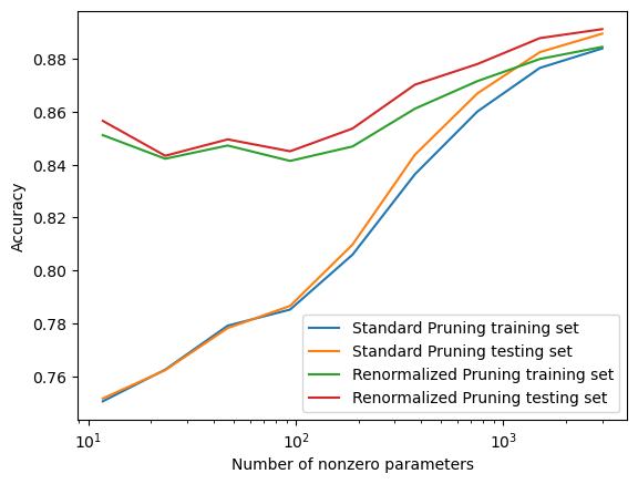
Figure 1: MNIST trained neural network. Plot of accuracy of neural network after sparsifying with versus without renormalization.

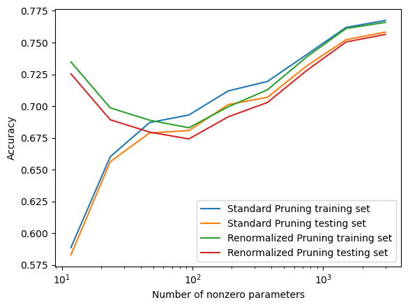
Figure 2: Fashion MNIST trained neural network. Plot of accuracy of neural network after sparsifying with versus without renormalization.

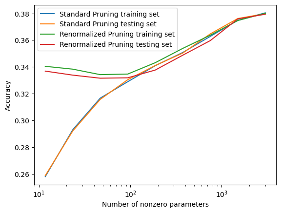
Figure 3: CIFAR-10 trained neural network. Plot of accuracy of neural network after sparsifying with versus without renormalization.

Note the logarithmic scales in the figures. We see that standard pruning decreases in accuracy quickly as sparsity increases, that is the number of nonzero parameters goes to zero. We also see that Renormalized Pruning maintains it’s accuracy much better in the high sparsity regime. We have not tested this method on the largest neural networks or the largest datasets due to computation constraints but we expect the same result due to the theorems above.

4 Conclusion

We have proposed the Renormalized Pruning method which is simple and fast to implement with the most common ‘one-shot’ pruning method. We proved that Renormalized Pruning has error that goes to 0 with concentration of neural network parameters and feature embeddings. Then we proved that standard pruning (via absolute value) has large error that doesn’t converge, with high probability. We, experimentally, see that the standard pruning accuracy decays in the very high sparsity regime, >90% sparsity. We experimentally test this method on three real world datasets: MNIST, Fashion MNIST, and CIFAR-10. We see that Renormalized Pruning drastically improves accuracy for high pruning levels. We believe that this is an important improvement in sparse neural network theory and that it is simple enough for anyone to immediately use.

Appendix A Appendix

Proof of Theorem 1.

Recall we let the renormalized $\widehat{\Phi}_{M}:=\frac{N}{N-M}\Phi_{M}$. Assume all $\phi_{i}$ are in the $\delta$ radius 2-Ball, $\phi_{i}\in B_{\delta}$, that is $\|\phi_{i}\|_{2}\leq\delta$. Let $a_{i}\in[\alpha,\beta]$ with $0<\alpha<\beta$ for each $i$ by absorbing the sign into $\phi_{i}$. Let $P$ be the set of indices pruned in $\Phi_{M}$.

Set $\gamma=M/(N-M)$.

$$\|\Phi-\widehat{\Phi}_{M}\|_{2}=\|\Phi-(1+\gamma)\Phi_{M}\|$$

$$=\left\|\sum_{i}a_{i}\phi_{i}-(1+\gamma)\sum_{j\notin P}a_{j}\phi_{j}\right\|$$

$$=\left\|\sum_{i\in P}a_{i}\phi_{i}-\gamma\sum_{j\notin P}a_{j}\phi_{j}\right\|$$

$$=\left\|\sum_{i\in P}\left(a_{i}\phi_{i}-\frac{\gamma}{M}\sum_{j\notin P}a_{j}\phi_{j}\right)\right\|$$

$$\leq\sum_{i\in P}\left\|a_{i}\phi_{i}-\frac{\gamma}{M}\sum_{j\notin P}a_{j}\phi_{j}\right\|$$

$$\leq\sum_{i\in P}\left\|a_{i}\phi_{i}-\frac{\gamma}{M}\sum_{j\notin P}a_{j}\phi_{j}-a_{i}\mu_{\phi}+a_{i}\mu_{\phi}\right\|$$

$$\leq\sum_{i\in P}\left\|a_{i}\phi_{i}-a_{i}\mu_{\phi}\right\|+\left\|a_{i}\mu_{\phi}-\frac{\gamma}{M}\sum_{j\notin P}a_{j}\phi_{j}\right\|$$

$$\leq\sum_{i\in P}a_{i}\Delta_{\phi}+\left\|\sum_{j\notin P}\frac{\gamma}{M}a_{j}\phi_{j}-\frac{a_{i}}{(N-M)}\mu_{\phi}\right\|$$

$$\leq\sum_{i\in P}a_{i}\Delta_{\phi}+\left\|\frac{a_{i}}{N-M}\sum_{j\notin P}\frac{a_{j}}{a_{i}}\phi_{j}-\mu_{\phi}\right\|$$

$$\leq\sum_{i\in P}a_{i}\Delta_{\phi}+\frac{a_{i}}{N-M}\sum_{j\notin P}\left\|\frac{a_{j}}{a_{i}}\phi_{j}-\mu_{\phi}\right\|$$

$$\leq\sum_{i\in P}a_{i}\Delta_{\phi}+\frac{a_{i}}{N-M}\sum_{j\notin P}\left\|\phi_{j}-\frac{a_{j}}{a_{i}}\phi_{j}\right\|+\left\|\phi_{j}-\mu_{\phi}\right\|$$

$$\leq\sum_{i\in P}a_{i}\Delta_{\phi}+\frac{a_{i}}{N-M}\sum_{j\notin P}\left\|1-\frac{a_{j}}{a_{i}}\right\|\|\phi_{j}\|+\Delta_{\phi}$$

$$\leq\sum_{i\in P}a_{i}\Delta_{\phi}+\frac{a_{i}}{N-M}\sum_{j\notin P}\left\|1-\frac{a_{j}}{a_{i}}\right\|\delta+\Delta_{\phi}$$

$$\leq\sum_{i\in P}a_{i}\Delta_{\phi}+\frac{a_{i}}{N-M}\sum_{j\notin P}\frac{(\beta-\alpha)(\beta+\alpha)}{\alpha\beta}\delta+\Delta_{\phi}$$

$$\leq\sum_{i\in P}a_{i}\Delta_{\phi}+a_{i}\frac{(\beta-\alpha)(\beta+\alpha)}{\alpha\beta}\delta+\Delta_{\phi}a_{i}$$

$$\leq 2\beta\Delta_{\phi}M+(\beta-\alpha)(\beta+\alpha)\delta M/\alpha$$

$$\leq O(\Delta_{\phi}+\xi)$$

as $\Delta_{\phi}+\xi\rightarrow 0$.

∎

Proof of Theorem 2.

We have that

$$\|\Phi-\Phi_{M}\|_{2}^{2}=\|\sum_{i\in P}a_{i}\phi_{i}\|_{2}^{2}$$

$$=\sum_{i\in P}a_{i}^{2}\langle\phi_{i},\phi_{i}\rangle+\sum_{i,j\in P,i\neq j}2a_{i}a_{j}\langle\phi_{i},\phi_{j}\rangle$$

$$=\delta^{2}\sum_{i\in P}a_{i}^{2}+\sum_{i,j\in P,i\neq j}2a_{i}a_{j}\langle\phi_{i},\phi_{j}\rangle$$

$$\geq\delta^{2}\sum_{i\in P}a_{i}^{2}-\sum_{i,j\in P,i\neq j}2a_{i}a_{j}\epsilon$$

$$\geq\delta^{2}\sum_{i\in P}a_{i}^{2}-\epsilon M^{2}\max_{i,j\in P,i\neq j}a_{i}a_{j}$$

$$\geq\delta^{2}\sum_{i\in P}a_{i}^{2}-\epsilon M^{2}\max_{i\in P}a_{i}^{2}.$$

∎

References

Ball [1997]
K. Ball.
An elementary introduction to modern convex geometry.
Flavors of geometry, 31(1-58):26, 1997.
Becker et al. [2016]
A. Becker, L. Ducas, N. Gama, and T. Laarhoven.
New directions in nearest neighbor searching with applications to
lattice sieving.
In Proceedings of the twenty-seventh annual ACM-SIAM symposium
on Discrete algorithms, pages 10–24. SIAM, 2016.
Grigas et al. [2019]
P. Grigas, A. Lobos, and N. Vermeersch.
Stochastic in-face frank-wolfe methods for non-convex optimization
and sparse neural network training.
arXiv preprint arXiv:1906.03580, 2019.
Hashemi et al. [2021]
A. Hashemi, H. Schaeffer, R. Shi, U. Topcu, G. Tran, and R. Ward.
Generalization bounds for sparse random feature expansions.
arXiv preprint arXiv:2103.03191, 2021.
doi: 10.48550/arXiv.2103.03191.
Krizhevsky [2009]
A. Krizhevsky.
Learning multiple layers of features from tiny images, 2009.
URL www.cs.toronto.edu/~kriz/cifar.html.
CIFAR-10.
LeCun et al. [1998]
Y. LeCun, C. Cortes, and C. J. Burges.
The mnist database of handwritten digits, 1998.
URL http://yann.lecun.com/exdb/mnist/.
Liu et al. [2015]
B. Liu, M. Wang, H. Foroosh, M. Tappen, and M. Pensky.
Sparse convolutional neural networks.
In Proceedings of the IEEE Conference on Computer Vision and
Pattern Recognition (CVPR), June 2015.
Louizos et al. [2017]
C. Louizos, M. Welling, and D. P. Kingma.
Learning sparse neural networks through regularization.
arXiv preprint arXiv:1712.01312, 2017.
Mao et al. [2017]
H. Mao, S. Han, J. Pool, W. Li, X. Liu, Y. Wang, and W. J. Dally.
Exploring the regularity of sparse structure in convolutional neural
networks.
arXiv preprint arXiv:1705.08922, 2017.
Matousek [2013]
J. Matousek.
Lectures on discrete geometry, volume 212.
Springer Science & Business Media, 2013.
Mei and Montanari [2022]
S. Mei and A. Montanari.
The generalization error of random features regression: Precise
asymptotics and the double descent curve.
Communications on Pure and Applied Mathematics, 75(4):667–766, 2022.
doi: 10.1002/cpa.22008.
Miao et al. [2021]
L. Miao, X. Luo, T. Chen, W. Chen, D. Liu, and Z. Wang.
Learning pruning-friendly networks via frank-wolfe: One-shot,
any-sparsity, and no retraining.
In International Conference on Learning Representations, 2021.
Xiao et al. [2017]
H. Xiao, K. Rasul, and R. Vollgraf.
Fashion-mnist: a novel image dataset for benchmarking machine
learning algorithms, 2017.
URL http://github.com/zalandoresearch/fashion-mnist.
Zimmer et al. [2022]
M. Zimmer, C. Spiegel, and S. Pokutta.
Compression-aware training of neural networks using frank-wolfe.
arXiv preprint arXiv:2205.11921, 2022.