Continuous boundary condition at the interface for two coupled fluids

Abstract

We consider two laminar incompressible flows coupled by the continuous law at a fixed interface $\Gamma_{I}$. We approach the system by one that satisfies a friction Navier law at $\Gamma_{I}$, and we show that when the friction coefficient goes to $\infty$, the solutions converges to a solution of the initial system. We then write a numerical Schwarz-like coupling algorithm and run 2D-simulations, that yields same convergence result.

MCS Classification: 76D07, 35J20, 65N30

Key-words: Stokes equations, coupled problems, variational formulation, numerical simulations.

1 Introduction

We consider the two coupled fluids problem with a rigid lid assumption, given by two 3D stokes equations,

(1.1) $$-\nu_{i}\Delta{\bf u}_{i}+\nabla p_{i}={\bf f}_{i},\quad\nabla\cdot{\bf u}_{i}=0,$$

(1.2) $${\bf u}_{1,h|\Gamma_{I}}={\bf u}_{2,h|\Gamma_{I}},\quad w_{i|\Gamma_{I}}={\bf u}_{i}\cdot{\bf n}_{i|\Gamma_{I}}=0,$$

(1.3) $${\bf u}_{1|\Gamma_{1}}={\bf u}_{2|\Gamma_{2}}=0,$$

for $i=1,2$, where the velocities $({\bf u}_{1},{\bf u}_{2})=({\bf u}_{1}({\bf x}_{h},z_{1}),{\bf u}_{2}({\bf x}_{h},z_{2}))$ are decomposed as ${\bf u}_{i}=({\bf u}_{i,h},w)$, ${\bf u}_{i,h}=(u_{i,x},u_{i,y})$. Moreover, ${\bf x}_{h}\in\mathbb{T}_{2}$, where $\mathbb{T}_{2}$ is the two dimensional torus, which means that we consider horizontal periodic boundary conditions. The interface $\Gamma_{I}$ is given by $\Gamma_{I}=\{({\bf x}_{h},0),{\bf x}_{h}\in\mathbb{T}_{2}\}$, the boundaries $\Gamma_{i}$ are given by $\Gamma_{1}=\{({\bf x}_{h},z_{1}^{+}),{\bf x}_{h}\in\mathbb{T}_{2}\}$, $\Gamma_{2}=\{({\bf x}_{h},z_{2}^{-}),{\bf x}_{h}\in\mathbb{T}_{2}\}$, $z_{1}\in J_{1}=[0,z_{1}^{+}]$, $z_{2}\in J_{2}=[z_{2}^{-},0]$, where $z_{1}^{+}>0$ and $z_{2}^{-}<0$. The coefficient $\nu_{i}>0$ is the viscosity of the fluid $i$, $p_{i}$ its pressure.

The main characteristic of this problem is the continuity boundary condition (1.2), which is natural and physical [2], and usually considered for free interfaces [6]. Notice that the rigid lid assumption we consider is reasonable for laminar coupled flows, as well as for large scales. In this paper we adress the question of the existence and uniqueness of a weak solution to Problem (1.1)-(1.2)-(1.3), given as the limit of ”frictional solutions”, for which we can write a numerical Schwarz-like algorithm. More specifically, we approach this problem by the following problem

(1.4) $$-\nu_{i}\Delta{\bf u}_{i}+\nabla p_{i}={\bf f}_{i},\quad\nabla\cdot{\bf u}_{i}=0,$$

(1.5) $$\nu_{i}\frac{\partial{\bf u}_{i,h}}{\partial{\bf n}_{i}}|_{\Gamma_{I}}=-\alpha({\bf u}_{i,h}-{\bf u}_{j,h}),\quad w_{i|\Gamma_{I}}={\bf u}_{i}\cdot{\bf n}_{i|\Gamma_{I}}=0,$$

(1.6) $${\bf u}_{i|\Gamma_{i}}=0,$$

$i,j=1,2$, in which the continuity condition (1.2) is replaced by the Navier law (1.5) where $i\not=j$. Similar problems have been already studied before, see [3, 4, 5, 8], and the existence and uniqueness of a weak solution is guaranteed. We aim to investigate how Problem (1.4)-(1.5)-(1.6) approaches Problem (1.1)-(1.2)-(1.3) when the friction coefficient $\alpha$ goes to infinity. Such question has already been adressed in [1] for a single fluid, where it is proved that the corresponding solution strongly converges to a solution to the corresponding Stokes (Navier-Stokes) equations with a no slip boundary condition when $\alpha\to\infty$. We show in this paper the convergence in $H^{1}$ space type of the solution of (1.4)-(1.5)-(1.6) to a solution of (1.1)-(1.2)-(1.3) (see Theorem 2.1).
As we shall see, numerical simulations are easily carried out by (1.4)-(1.5)-(1.6) thanks to a Schwarz-like coupling algorithm, that does not work for (1.1)-(1.2)-(1.3). This method has already been successfully implemented for coupled problems, see for example [9].

The note is organized as follows. In the first part we set the functional framework and then we prove the convergence result, namely Theorem 2.1. In the second part, we describe our algorithm and show some numerical results in the 2D case. In particular we check the numerical convergence of the algorithm.

2 Convergence analysis

2.1 Energy balance

This section is devoted to the derivation of the main a priori estimate, which is standard. Let $({\bf u}_{1},{\bf u}_{2})$ be any enough smooth solution to Problem (1.4)-(1.5)-(1.6). Taking the scalar product of equation (1.4)_i by ${\bf u}_{i}$ in integrating over $\mathbb{T}_{2}\times J_{i}$ over yields by (1.6)_i, because of the periodic boundary conditions in the $x-y$ axes, the incompressibility condition and ${\bf u}_{i}\cdot{\bf n}_{i}=0$ at $\Gamma_{I}$,

$$\nu_{i}\displaystyle\int_{\mathbb{T}_{2}\times J_{i}}|\nabla{\bf u}_{i}|^{2}-\nu_{i}\displaystyle\int_{\Gamma_{I}}\frac{\partial{\bf u}_{i,h}}{\partial{\bf n}_{i}}=\displaystyle\int_{\mathbb{T}_{2}\times J_{i}}{\bf f}_{i}\cdot{\bf u}_{i},$$

giving by (1.5), $\nu_{i}\displaystyle\int_{\mathbb{T}_{2}\times J_{i}}|\nabla{\bf u}_{i}|^{2}+\alpha\displaystyle\int_{\Gamma_{I}}{\bf u}_{i,h}\cdot({\bf u}_{i,h}-{\bf u}_{j,h})=\displaystyle\int_{\mathbb{T}_{2}\times J_{i}}{\bf f}_{i}\cdot{\bf u}_{i}.$ Summing up the two equalities yields the following energy balance,

(2.1) $$\begin{array}[]{l}\nu_{1}\displaystyle\int_{\mathbb{T}_{2}\times J_{1}}|\nabla{\bf u}_{1}|^{2}+\nu_{2}\displaystyle\int_{\mathbb{T}_{2}\times J_{2}}|\nabla{\bf u}_{2}|^{2}+\alpha\displaystyle\int_{\Gamma_{I}}|{\bf u}_{1,h}-{\bf u}_{2,h}|^{2}=\\ \hskip 227.62204pt\displaystyle\int_{\mathbb{T}_{2}\times J_{1}}{\bf f}_{1}\cdot{\bf u}_{1}+\displaystyle\int_{\mathbb{T}_{2}\times J_{2}}{\bf f}_{2}\cdot{\bf u}_{2}.\end{array}$$

2.2 Functions spaces, variational formulation

Let ${\cal W}_{i}=\{{\bf u}\in C^{\infty}(\mathbb{T}_{2}\times J_{i}),~{}~{}{\bf u}_{|\Gamma_{i}}=0,~{}~{}{\bf u}\cdot{\bf n}_{i}|_{\Gamma_{I}}=0,~{}~{}\nabla\cdot{\bf u}_{i}=0\},$ equipped with $||{\bf u}||_{i,1}=||\nabla{\bf u}||_{L^{2}(\mathbb{T}_{2}\times J_{i})}$ which is indeed a norm due to the condition ${\bf u}_{|\Gamma_{i}}=0$. Let $W_{i}$ denotes the completion of ${\cal W}_{i}$ with respect to this norm,

(2.2) $$W=W_{1}\times W_{2},\quad W_{0}=\{({\bf u}_{1},{\bf u}_{2})\in W,\,\,{\bf u}_{1,h|\Gamma_{I}}={\bf u}_{2,h|\Gamma_{I}}\,a.e.\hbox{ in }\Gamma_{I}\}.$$

We equip $W$ with the scalar product, for any ${\bf U}=({\bf u}_{1},{\bf u}_{2}),{\bf V}=({\bf v}_{1},{\bf v}_{2})\in W$,

(2.3) $$\Lambda({\bf U},{\bf V})=\nu_{1}\displaystyle\int_{\mathbb{T}_{2}\times J_{1}}\nabla{\bf u}_{1}\cdot\nabla{\bf v}_{1}+\nu_{2}\displaystyle\int_{\mathbb{T}_{2}\times J_{2}}\nabla{\bf u}_{2}\cdot\nabla{\bf v}_{2}.$$

The space $W_{0}$ is the kernel of the form $L:({\bf u}_{1},{\bf u}_{2})\to{\bf u}_{1,h|\Gamma_{I}}-{\bf u}_{2,h|\Gamma_{I}}$, which is continuous by the trace theorem. Therefore $W_{0}$ is a closed hyperplane of $W$. Let $P$ denotes the orthogonal projection over $W_{0}$, and ${\boldsymbol{\Phi}}=({\boldsymbol{\phi}}_{1},{\boldsymbol{\phi}}_{2})$ a unit orthogonal vector to $W_{0}$, so that $W_{0}^{\perp}=\operatorname{vect}{\boldsymbol{\Phi}}$.

Definition 2.1.

(weak solution) A couple ${\bf U}=({\bf u}_{1},{\bf u}_{2})\in W$ is a weak solution to Problem (1.4)-(1.5)-(1.6) when $\forall\,{\bf V}=({\bf v}_{1},{\bf v}_{2})\in W$,

(2.4) $$\Lambda({\bf U},{\bf V})+\alpha\displaystyle\int_{\Gamma_{I}}({\bf u}_{1,h}-{\bf u}_{2,h})\cdot({\bf v}_{1,h}-{\bf v}_{2,h})=\displaystyle\int_{\mathbb{T}_{2}\times J_{1}}{\bf f}_{1}\cdot{\bf v}_{1}+\displaystyle\int_{\mathbb{T}_{2}\times J_{2}}{\bf f}_{2}\cdot{\bf v}_{2}=({\bf F},{\bf V}).$$

Throughout the rest of the paper, we assume that ${\bf f}_{i}\in L^{2}(\mathbb{T}_{2}\times J_{i})$, $i=1,2$. The existence and the uniqueness of a weak solution to Problem (1.4)-(1.5)-(1.6) that satisfies the energy balance (2.1) is straightforward by the Lax-Milgram Theorem for any given $\alpha>0$. Notice that work remains to be done about the pressures, by a suitable adaptation of a De Rham like theorem in this framework, which is an open problem.

2.3 Convergence

Let ${\bf U}_{\alpha}=({\bf u}_{1}^{\alpha},{\bf u}_{2}^{\alpha})\in W$ be the solution of (1.4)-(1.5)-(1.6). We study in this section the convergence of the familly $({\bf U}_{\alpha})_{\alpha>0}$ when $\alpha\to\infty$, proving the following result.

Theorem 2.1.

The familly $({\bf U}_{\alpha})_{\alpha>0}$ strongly converges in $W$ to a weak solution ${\bf U}=({\bf u}_{1},{\bf u}_{2})\in W_{0}$ of Problem (1.1)-(1.2)-(1.3) when $\alpha\to\infty$, in the sense:

(2.5) $$\forall\,{\bf V}=({\bf v}_{1},{\bf v}_{2})\in W_{0},\quad\Lambda({\bf U},{\bf V})=({\bf F},{\bf V}).$$

Moreover, the solution of (2.5) is unique.

Proof.

Let ${\bf U}^{\alpha}=({\bf u}_{1}^{\alpha},{\bf u}_{2}^{\alpha})\in W=W_{1}\times W_{2}$ be the solution of $(S_{1},S_{2})$. We first show that the familly $({\bf U}^{\alpha})_{\alpha>0}$ is bounded in $W$. We have, by (2.1),

(2.6) $$\|{\bf U}^{\alpha}\|_{W}^{2}+\alpha\displaystyle\int_{\Gamma_{I}}|{\bf u}_{1,h}^{\alpha}-{\bf u}_{2,h}^{\alpha}|^{2}=\displaystyle\int_{\mathbb{T}_{2}\times J_{1}}{\bf f}_{1}\cdot{\bf u}_{1}^{\alpha}+\displaystyle\int_{\mathbb{T}_{2}\times J_{2}}{\bf f}_{2}\cdot{\bf u}_{2}^{\alpha},$$

which yields

(2.7) $$\|{\bf U}^{\alpha}\|_{W}^{2}\leq\displaystyle\int_{\mathbb{T}_{2}\times J_{1}}{\bf f}_{1}\cdot{\bf u}_{1}^{\alpha}+\displaystyle\int_{\mathbb{T}_{2}\times J_{2}}{\bf f}_{2}\cdot{\bf u}_{2}^{\alpha}.$$

We deduce from Poincaré and Cauchy-Schwarz inequalities that $({\bf U}^{\alpha})_{\alpha>0}$ is indeed bounded in $W$. Therefore, we can extract a subsequence $({\bf U}^{\alpha_{n}})_{n\in{\rm I}\hskip-2.41849pt{\rm N}}$ ($\alpha_{n}\to\infty$ as $n\to\infty$) which converges weakly in $W$ to some $U\in W$. Moreover, by the trace theorem and usual Sobolev compactness results, the corresponding traces are strongly convergent in $L^{2}(\Gamma_{I})$. As by (2.6) $\lim_{n\to\infty}tr({\bf u}_{1,h}^{\alpha_{n}}-{\bf u}_{2,h}^{\alpha_{n}})=0$ in $L^{2}(\Gamma_{I})$, then $U\in W_{0}$. Finally, take ${\bf V}\in W_{0}$ in (2.4) as test, so that the boundary term vanishes. By passing to the limit in this case when $\alpha\to\infty$, we obtain that $U$ is a weak solution to (1.1)-(1.2)-(1.3). Uniqueness is straightforward, which in addition garanties that the entire familly does converge to ${\bf U}$.

It remains to show the strong convergence. Let $\lambda_{\alpha}\in{\rm I}\hskip-2.41849pt{\rm R}$, be such that ${\bf U}^{\alpha}=P{\bf U}^{\alpha}+\lambda_{\alpha}{\bf\Phi}$ (${\bf\Phi}$ being given in section 2.2). We first show the strong convergence of $(P{\bf U}^{\alpha})_{\alpha>0}$ to ${\bf U}$ by taking $P{\bf U}^{\alpha}$ as a test in (2.4) which gives, by using the orthogonal decomposition of ${\bf U}^{\alpha}$,

(2.8) $$\Lambda({\bf U}^{\alpha},P{\bf U}^{\alpha})=\|P{\bf U}^{\alpha}\|_{W}^{2}=({\bf F},P{\bf U}^{\alpha}),$$

since the boundary term on $\Gamma_{I}$ equals to zero by orthogonality. Therefore $(P{\bf U}^{\alpha})_{\alpha>0}$ is bounded in $W_{0}$, then converges weakly -up to a subsequence (keeping the same notation)- to a limit ${\bf W}$, strongly in $L^{2}((\mathbb{T}_{2}\times J_{1})\times(\mathbb{T}_{2}\times J_{2}))$. Taking ${\bf V}\in W_{0}$ in (2.4) as test, noting that in this case $\Lambda({\bf U}^{\alpha},{\bf V})=\Lambda(P{\bf U}^{\alpha},{\bf V})$, and passing to the limit when $\alpha\to\infty$, we see that ${\bf W}$ is solution of the problem (1.1)-(1.2)-(1.3), hence ${\bf W}={\bf U}$ by uniqueness, and the entire sequence converges. Therefore, passing to the limit in (2.8) yields

$$\lim_{\alpha\to\infty}||P{\bf U}^{\alpha}||^{2}_{W}=({\bf F},{\bf U})=\Lambda({\bf U},{\bf U})=||{\bf U}||_{W}^{2},$$

which, together with the weak convergence, ensures the strong convergence as claimed. To conclude, it remains to prove that $\lim_{\alpha\to\infty}\lambda_{\alpha}=0$. By the energy balance (2.6), we have

(2.9) $$\limsup_{\alpha\to\infty}||{\bf U}^{\alpha}||^{2}_{W}+\limsup_{\alpha\to\infty}\alpha\int_{\Gamma_{I}}|{\bf u}_{1,h}^{\alpha}-{\bf u}_{2,h}^{\alpha}|^{2}=({\bf F},{\bf U}).$$

However, we have $\int_{\Gamma_{I}}|{\bf u}_{1,h}^{\alpha}-{\bf u}_{2,h}^{\alpha}|^{2}=\lambda^{2}_{\alpha}\int_{\Gamma_{I}}|\boldsymbol{\phi}_{1,h}-\boldsymbol{\phi}_{1,h}|^{2}$. Therefore, since $(||{\bf U}_{\alpha}||^{2}_{W})_{\alpha>0}$ is bounded, by (2.9) we have $(\alpha\lambda_{\alpha}^{2})_{\alpha>0}$ is bounded, which can happen only if $\lambda_{\alpha}\to 0$ as $\alpha\to\infty$, concluding the proof. ∎

3 Numerical simulations

3.1 Algorithm

We solve the problems (1.4)-(1.5)-(1.6) for large values of $\alpha$, with a coupling Schwarz like algorithm, using the software Freefem++, for solving 2D Stokes problems by the finite element method. Our algorithm is set as follows.
Step 1: We solve the problem on the upper part which gives a first value ${\bf u}_{1}^{\alpha,0}$.

(3.1) $$-\nu_{1}\Delta{\bf u}_{1}^{\alpha,0}+\nabla P_{1}^{(0)}={\bf f}_{1},\quad\nabla\cdot{\bf u}_{1}^{\alpha,0}=0,$$

(3.2) $$\nu_{1}\frac{\partial{\bf u}_{1,h}^{\alpha,0}}{\partial{\bf n}_{1}}|_{\Gamma_{I}}=-\alpha{\bf u}_{1,h}^{\alpha,0},$$

(3.3) $${\bf u}_{1,h}^{\alpha,0}|_{\Gamma_{1}}=0,\quad{\bf u}_{1,h}^{\alpha,0}\cdot{\bf n}_{1}=0.$$

This velocity allows us to solve the problem on the lower part, and to calculate the velocities step by step, up and down.

Step 2: We calculate ${\bf u}_{2}^{\alpha,n}$ and ${\bf u}_{1}^{\alpha,n+1}$ by solving

(3.4) $$-\nu_{2}\Delta{\bf u}_{2}^{\alpha,n}+\nabla P_{2}^{(n)}={\bf f}_{2},\quad\nabla\cdot{\bf u}_{2}^{\alpha,n}=0,$$

(3.5) $$\nu_{2}\frac{\partial{\bf u}_{2,h}^{\alpha,n}}{\partial{\bf n}_{2}}|_{\Gamma_{I}}=-\alpha({\bf u}_{2,h}^{\alpha,n}-{\bf u}_{1,h}^{\alpha,n}),$$

(3.6) $${\bf u}_{2,h}^{\alpha,n}|_{\Gamma_{2}}=0,\quad{\bf u}_{2,h}^{\alpha,n}\cdot{\bf n}_{2}=0.$$

and

(3.7) $$-\nu_{1}\Delta{\bf u}_{1}^{\alpha,n+1}+\nabla P_{1}^{(n+1)}={\bf f}_{1},\quad\nabla\cdot{\bf u}_{1}^{\alpha,n+1}=0,$$

(3.8) $$\nu_{1}\frac{\partial{\bf u}_{1,h}^{\alpha,n+1}}{\partial{\bf n}_{1}}|_{\Gamma_{I}}=-\alpha({\bf u}_{1,h}^{\alpha,n+1}-{\bf u}_{2,h}^{\alpha,n}),$$

(3.9) $${\bf u}_{1,h}^{\alpha,n+1}|_{\Gamma_{1}}=0,\quad{\bf u}_{1,h}^{\alpha,n+1}\cdot{\bf n}_{1}=0.$$

Note that we are able to prove the stability of this algorithm, and numerical simulation confirm the convergence (see table below). Problem (1.1)-(1.2)-(1.3) cannot be solved in a similar way. Indeed, the interface conditions

(3.10) $${\bf u}_{2,h}^{(n)}|_{\Gamma_{I}}={\bf u}_{1,h}^{(n)}|_{\Gamma_{I}},\quad{\bf u}_{1,h}^{(n+1)}|_{\Gamma_{I}}={\bf u}_{2,h}^{(n)}|_{\Gamma_{I}},$$

imply that the sequences $({\bf u}_{1,h}^{(n)})_{n}$ and $({\bf u}_{2,h}^{(n)})_{n}$ are constant on the interface $\Gamma_{I}$ which doesn’t allow any iterations on the coupling algorithm.

3.2 Simulation results

We take $z_{1}^{+}=50$ , $z_{2}^{-}=-5$, $L=100$, $\nu_{1}=\nu_{2}=1$ and the source ${\bf F}=\left(\begin{pmatrix}1\\ -1\end{pmatrix},\begin{pmatrix}1\\ -1\end{pmatrix}\right)$ constant, for the simplicity.

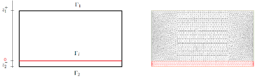
Figure 1: Domain and mesh

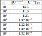
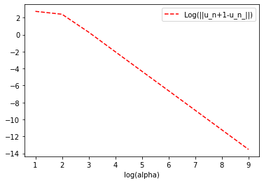
Figure 2: L2 norm of the errors and rate of convergence for n=100

$\alpha$	$n$
$10$	$4026$
$10^{2}$	$984$
$10^{3}$	$408$
$10^{4}$	$221$
$10^{5}$	$137$
$10^{6}$	$54$
$10^{9}$	$9$

To check the numerical convergence of the method, we study the error term $\|{\bf U}^{\alpha,n+1}-{\bf U}^{\alpha,n}\|_{L^{2}}$. On the left, for a given $\alpha$, we have the first value of $n$ for which $\|{\bf U}^{\alpha,n+1}-{\bf U}^{\alpha,n}\|_{L^{2}}<10^{-3}$. The method is always converging, and the convergence is almost instantaneous for large $\alpha$ $(>10^{6})$.

Figure 3: Velocities, $f_{1}=(1,-1)=f_{2}$, $n=9$, $\alpha=10^{9}$

References

- [1] P. Acevedo Tapia, C. Amrouche, C. Conca, and A. Ghosh. Stokes and Navier-Stokes equations with Navier boundary conditions. J. Differential Equations, 285:258–320, 2021.
- [2] G. K. Batchelor. An introduction to fluid dynamics. Cambridge Mathematical Library. Cambridge University Press, Cambridge, paperback edition, 1999.
- [3] C. Bernardi, T. Chacón Rebollo, R. Lewandowski, and F. Murat. A model for two coupled turbulent fluids. I. Analysis of the system. In Nonlinear partial differential equations and their applications. Collège de France Seminar, Vol. XIV (Paris, 1997/1998), volume 31 of Stud. Math. Appl., pages 69–102. North-Holland, Amsterdam, 2002.
- [4] Jeffrey M. Connors. Partitioned time discretization for atmosphere-ocean interaction. ProQuest LLC, Ann Arbor, MI, 2010. Thesis (Ph.D.)–University of Pittsburgh.
- [5] Jeffrey M. Connors, Jason S. Howell, and William J. Layton. Partitioned time stepping for a parabolic two domain problem. SIAM J. Numer. Anal., 47(5):3526–3549, 2009.
- [6] David Lannes. A stability criterion for two-fluid interfaces and applications. Arch. Ration. Mech. Anal., 208(2):481–567, 2013.
- [7] F. Legeais and R. Lewandowski. In preparation. 2022.
- [8] Jacques-Louis Lions, Roger Temam, and Shou Hong Wang. Mathematical theory for the coupled atmosphere-ocean models. (CAO III). J. Math. Pures Appl. (9), 74(2):105–163, 1995.
- [9] M. Tayachi, A. Rousseau, E. Blayo, N. Goutal, and V. Martin. Design and analysis of a Schwarz coupling method for a dimensionally heterogeneous problem. Internat. J. Numer. Methods Fluids, 75(6):446–465, 2014.