Algebraic Biochemistry: a Framework for Analog Online Computation in Cells

Abstract

The Turing completeness of continuous chemical reaction networks (CRNs) states that any computable real function can be computed by a continuous CRN on a finite set of molecular species, possibly restricted to elementary reactions, i.e. with at most two reactants and mass action law kinetics. In this paper, we introduce a notion of online analog computation for the CRNs that stabilize the concentration of their output species to the result of some function of the concentration values of their input species, whatever changes are operated on the inputs during the computation. We prove that the set of real functions stabilized by a CRN with mass action law kinetics is precisely the set of real algebraic functions.

1 Introduction

Chemical Reaction Networks (CRNs) are a standard formalism used in chemistry and biology to describe complex molecular interaction systems. In the perspective of systems biology, they are a central tool to analyze the high-level functions of the cell in terms of their low-level molecular interactions. In that perspective, the Systems Biology Markup Language (SBML) [19] is a common format to exchange CRN models and build CRN model repositories, such as Biomodels.net [5] which contains thousands of CRN models of a large variety of cell biochemical processes. In the perspective of synthetic biology, they constitute a target programming language to implement in chemistry new functions either in vitro, e.g. using DNA polymers [20], or in living cells using plasmids [10] or in artificial vesicles using proteins [8].

The mathematical theory of CRNs was introduced in the late 70’s, on the one hand by Feinberg in [15], by focusing on perfect adaptation properties and multistability analyses [9], and on the other hand, by Érdi and Tóth by characterizing the set of Polynomial Ordinary Differential Equation systems (PODEs) that can be defined by CRNs with mass action law kinetics, using dual-rail encoding for negative variables [11].

More recently, a computational theory of CRNs was investigated by formally relating their Boolean, discrete, stochastic and differential semantics in the framework of abstract interpretation [14], and by studying the computational power of CRNs under those different interpretations [7, 6, 12].

In particular, under the continuous semantics of CRNs interpreted by ODEs, the Turing-completeness result established in [12] states that any computable real function, i.e. computable by a Turing machine with an arbitrary precision given in input, can be computed by a continuous CRN on a finite set of molecular species, using elementary reactions with at most two reactants and mass action law kinetics. This result uses the following notion of analog computation of a non-negative real function computed by a CRN, where the result is given by the concentration of one species, $y_{1}$, and the error is controlled by the concentration of one second species, $y_{2}$:

Definition 1

[12] A function $f:\mathbb{R_{+}}\to\mathbb{R_{+}}$ is CRN-computable if there exist a CRN over some molecular species $\{y_{1},...,y_{n}\}$, and a polynomial $q\in\mathbb{R_{+}}^{n}[\mathbb{R_{+}}]$ defining their initial concentration values, such that for all $x\in\mathbb{R_{+}}$ there exists some (necessarily unique) function $y:\mathbb{R}\to\mathbb{R}^{n}$ such that $y(0)=q(x),\ y^{\prime}(t)=p(y(t))$ and for all $t>1$

$$|y_{1}(t)-f(x)|\leq y_{2}(t),$$

$y_{2}(t)\geq 0$, $y_{2}(t)$ is decreasing and $\lim_{t\to\infty}y_{2}(t)=0$.

From the theoretical point of view of computability, the control of the error which is explicitly represented in the above definition by the auxiliary variable $y_{2}$, is necessary to decide when the result is ready for a requested precision, and to mathematically define the function computed by a CRN if any.

From a practical point of view however, precision is of course an irrelevant issue since chemical reactions are stochastic in nature and the stability of the CRN and robustness with respect to the concentration species variations is a more important criterion than the precision of the result. With this provision to omit error control, the Turing-completeness result of continuous CRNs was used in [12] to design a compilation pipeline to implement any mathematical elementary function in abstract chemistry. This compiler, implemented in our CRN modeling, analysis and synthesis software Biocham [2] as the one presented here, generates a CRN over a finite set of abstract molecular species, through several symbolic computation steps, mainly composed of polynomialization [17], quadratization [16] and lazy dual-rail encoding of negative variables. A similar approach is undertaken in the CRN$++$ system [22], also related to[3].

Now, it is worth remarking that in the definition above, and in our implementation in Biocham, the input is defined by the initial concentration of the input species which may be consumed by the synthesized CRN to compute the result. This marks a fundamental difference with many natural CRNs which perform a kind of online computation by adapting the response to the evolution of the input. This is the case for instance of the ubiquitous MAPK signaling network which computes an input/output function well approximated by a Hill function of order 4.9 [18], while our synthesized CRNs to compute the same function consume their input and do not correctly adapt to change of the input value during computation [17].

In this paper, we are interested in a notion of online computation for continuous CRNs, by opposition to our previous notion of static computation of the result of a function for any initially given input. Our main theorem shows that the set of input/output functions stabilized online by a CRN with mass action law kinetics, is precisely the set of real algebraic functions.

Example 1

We can illustrate this result with a simple example. Let us consider a cell that produces a receptor, $I$, which is transformed in an active form, $A$, when bound to an external ligand $L$, and which stays active even after unbinding:

$$\begin{aligned} L+I&\rightarrow L+A\\ \emptyset&\leftrightarrow I\\ A&\rightarrow\emptyset\end{aligned}$$ (1)

The differential semantics with mass action law of unitary rate constant is the PODE:

$$\begin{aligned} \frac{dI}{dt}&=1-I-LI\\ \frac{dA}{dt}&=LI-A\\ \frac{dL}{dt}&=0\end{aligned}$$ (2)

At steady state, all the derivatives are null and by eliminating $I$, we immediately obtain the polynomial equation: $L-LA-A=0$. Thinking of this simple CRN as a kind of signal processing with the ligand as input and the active receptor as output, it is possible to find a polynomial relation between the input and the output. In this case, this relation entirely defines the function computed by the CRN:

$$A(L)=\frac{L}{1+L}.$$

For a given concentration of ligand, this is the only stable state of the system, independently of the initial concentrations of $A$ or $I$. This is why we say that the CRN stabilizes the function.

Such functions, for which there exists a polynomial relation between the inputs and output, are called algebraic functions in mathematics. We show here that the set of real algebraic functions is precisely the set of input/output functions stabilized by CRNs with mass action law kinetics. Furthermore, our constructive proof provides a compilation method to generate a stabilizing CRN for any real algebraic curve, i.e. any curve defined by the zeros of some polynomial.

1.1 Related work

Our CRN synthesis results can be compared to the ones of Buisman & al. who present in [1] a method to implement any algebraic expression by an abstract CRN. They rely on a direct expression of the function and a compilation process that mimics the composition of the elementary algebraic operations. We improve their results in three directions. First, our compilation pipeline is able to generate stabilizing CRNs for any algebraic function, including those algebraic functions that cannot be defined by algebraic expressions, such as the Bring radical (see Ex. 6). Second, our theoretical framework shows that the general set of algebraic functions precisely characterizes the set of functions that can be stably computed online by a CRN. Third, the quadratization and lazy-negative optimization algorithms presented in this paper allow us to generate more concise CRNs. On the example given in section 3.4 of [1] for the quadratic expression

$$y=\frac{b-\sqrt{b^{2}-4ac}}{2a}$$

used to find the root of a polynomial of second order, our compiler generates a CRN of $7$ species (including the $3$ inputs) and $11$ reactions, while their CRN following the syntax of the expression uses $10$ species and $14$ reactions. Moreover, our dual-rail encoding allows us to give correct answers for negative values of $y$.

2 Definitions and Main Theorem

For this article, we denote single chemical species with lower case letters and set of species with upper case letters, e.g. $X=\{x_{1},x_{2},\ldots\}$. By abuse of notation, we will use the same symbol for the variables of the ODEs, the chemical species and their concentrations, the context being sufficient to remove any ambiguity.

2.1 Chemical Reaction Networks

A chemical reaction with mass action law kinetics is composed of a multiset of reactants, a multiset of products and one rate constant. Such a reaction can be written as follows:

$$a+b\xrightarrow{k}2a$$ (3)

where $k$ is the rate constant, and the multisets are represented by linear expressions in which the (stoichiometric) coefficients give the multiplicity of the species in the multisets, here 2 for the product $a$, the coefficients equal to 1 being omitted. In this example, the velocity of the reaction is the product $kab$, i.e. the rate constant $k$ times the concentration of the reactants, $a$ and $b$.

In this paper, we consider CRNs with mass action law kinetics only. It is well known that the other kinetics, such as Michaelis-Menten or Hill kinetics, can be derived by quasi-steady state or quasi-equilibrium reductions of more complex CRNs with mass action kinetics [21]. Furthermore, the Turing-completeness of this setting [12] shows that there is no loss of generality with that restriction.

We also study the case where one or several species, called pinned (input) species, are present in such a way that their concentrations remain constant, independently of the activity of the CRN under study.

Definition 2

The differential semantics of a CRN with a distinguished set of pinned species $S^{p}$, is composed of the usual ODEs for the non pinned species $s\notin S^{p}$, and null differential functions for the pinned species:

$$\forall s\in S^{p},\quad\frac{ds}{dt}=0.$$ (4)

This pinning process may be due to a scale separation between the different concentrations (one of the species is so abundant that the CRN essentially do not modify its concentration), to a scale separation of volume (e.g. a compartment within a cell and a freely diffusive small molecule) or to an active mechanism ensuring perfect adaptation (e.g. the input is produced and consumed by some external reactions faster than the CRN itself, thus locking its concentration).

2.2 Stabilization

We are interested in the case where one particular species of the CRN, called the output, is such that, whatever moves the inputs may do, once the inputs are fixed, the concentration of the output species stabilizes on the result of some function of the fixed inputs. Furthermore, we want this value to be robust to small perturbations of both the auxiliary variables and the output. Of course, if the inputs are modified, the output has to be modified. The output thus encodes a particular kind of robust computation of a function which we shall call stabilization.

Definition 3

We say that a CRN over a set of $m+1+n$ species $\{X,y,Z\}$ with pinned inputs $X$ of cardinality $m$ and distinguished outputs $y$, stabilizes the function $f:I\mapsto\mathbb{R}_{+}$, with $I\subset\mathbb{R}_{+}^{m}$, over the domain ${\cal D}\subset\mathbb{R}_{+}^{m+1+n}$ if:

1. $\forall X^{0}\in I$ the restriction of the domain ${\cal D}$ to the slice $X=X^{0}$ is of plain dimension $n+1$, and

2. $\forall(X^{0},y^{0},Z^{0})\in{\cal D}$ the Polynomial Initial Value Problem (PIVP) given by the differential semantic with pinned input species $X$ and the initial conditions $X^{0},y^{0},Z^{0}$ is such that: $\lim_{t\rightarrow\infty}y(t)=f(X).$

This definition is extended to functions of $\mathbb{R}^{n}$ in $\mathbb{R}$ by dual-rail encoding [11]: for a CRN over the species $\{X^{+},X^{-},y^{+},y^{-},Z\}$ we ask that $\lim_{t\rightarrow\infty}(y^{+}-y^{-})(t)=f(X^{+}-X^{-}),$ for all initial conditions in the validity domain ${\cal D}$.

Let ${\cal F}_{S}$ be the set of functions stabilized by a CRN.

Several remarks are in order. A first remark concerns the fact that we ask for a domain ${\cal D}$ of plain dimension $n+1$, i.e. non-null measure in $\mathbb{R}^{n+1}$. That constraint is imposed in order to benefit from a strong form of robustness: there exists an open volume containing the desired fixed point such that it is the unique attractor in this space. Hence in this setting, minor perturbations are always corrected. This requirement of an isolated fixed point also impedes from hiding information in the initial conditions. The following example illustrates the crucial importance of that condition on the dimension of the domain ${\cal D}$

Example 2

The following PODE is constructed in such a way that $z_{2}$ goes exponentially to $x$ while $y$ and $z_{1}$ remain equal to $\cos(z_{2})$ and $\sin(z_{2})$ respectively.

$$\begin{aligned} \frac{dx}{dt}&=0,\quad&x(t=0)=\text{input}\\ \frac{dy}{dt}&=-z_{1}(x-z_{2})\quad&y(t=0)=1\\ \frac{dz_{1}}{dt}&=y(x-z_{2})\quad&z_{1}(t=0)=0\\ \frac{dz_{2}}{dt}&=(x-z_{2})\quad&z_{2}(t=0)=0\\ \end{aligned}$$ (5)

One might think that this PODE stabilizes the cosine as we have $\lim y(t)=cos(x)$ for any value of $x$. But cosine is not an algebraic function, and indeed, the only requirement for this PODE to be at steady state is: $x=z_{2}$, meaning that there exist fixed points for any value of $z_{1}$ and $x$. So this PODE does not stabilize the cosine function. The reason is that the cosine computation is encoded in the initial state. It is only for the domain where $y=\cos(z_{2})$ and $z_{1}=\sin(z_{2})$ that the computation works, but this domain is of null measure in $\mathbb{R}^{3}$ which breaks the first condition of Def. 3.

A second remark is that since the inputs are fixed in our semantics (they are by definition pinned species), the target of the output species which is the result $f(X)$ of some function $f$ is not a fluctuating goal: it is fixed by the initial conditions. In practice, what we ask is that the dynamics of the ODE for the slice of the domain ${\cal D}$ defined by imposing the inputs have a unique attractor satisfying $y=f(X^{0})$. But as we do not impose any constraint on the other variables ($Z$), we cannot speak of a fixed point since the dynamics on the other variables may not stabilize (e.g. oscillations, divergence, etc.). We will nevertheless speak of these object as pseudo-fixed point. If we start from a point on this pseudo fixed point, we will have: $\forall t,y(t)=f(X^{0})$.

A third remark is that our definition implies that apart from a transient behaviour of characteristic time $\tau$, the whole system is constrained to live in, or nearby, the subspace defined by $y=f(X)$. What is interesting is that if the inputs are themselves varying with a characteristic time that is slower than $\tau$, the output will follow those variations, hence preserving our desired property up to an error coming from the delay as long as the system stays in the domain ${\cal D}$. In a synthetic biology perspective, it is in principle possible to use a time-rescaling to modify the value of $\tau$. While a small $\tau$ allows for a faster adaptation, this usually comes at the expense of a greater energetic cost as the proteins turn-over tends to increase.

2.3 Algebraic Curves and Algebraic Functions

In mathematics, an algebraic curve (or surface) is the zero set of a polynomial in two (or more) variables. It is a usual convention in mathematics to speak indifferently of the polynomial and the curve it defines, seen as the same object. For instance, $x^{2}+y^{2}-1$ is seen as the unit circle.

Any polynomial $P$ can be expressed as a product of irreducible polynomials, i.e. polynomials that cannot be further factorized, up to a constant $k$:

$${P=k.\prod_{i=1\dots n}P_{i}^{a_{i}}}.$$

The $P_{i}$’s are called the components of $P$, and $a_{i}$ the multiplicity of $P_{i}$. We say that $P$ is in reduced form if all the components have multiplicity one, $\forall i\ a_{i}=1$. This is justified by one important result of algebraic geometry: in an algebraic closed field, such as the complex numbers $\mathbb{C}$, the set of points of an algebraic curve given with their multiplicity, suffices to define the polynomial in reduced form. This makes algebraic geometry an elegant and powerful theory.

In a non-algebraically closed field such as $\mathbb{R}$, a polynomial may have no real root. This difficulty is however irrelevant to us in this paper since we start with an algebraic real function, thus assuming the existence of real roots. For the purpose of this article, this fundamental result provides a canonical correspondence between an algebraic real function and its polynomial of minimal degree, i.e. a polynomial in reduced form, up to a multiplicative factor.

Definition 4

A function $f:I\subset\mathbb{R}^{m}\mapsto\mathbb{R}$ is algebraic if there exists a polynomial $P$ of $m+1$ variables such that:

$$\forall X\in I,P(X,f(X))=0.$$ (6)

We denote ${\cal F}_{A}$ the set of real algebraic functions.

We shall prove the following central theorem:

Theorem 2.1

The set of functions stabilized by a CRN with mass action law kinetics is the set of algebraic real functions: ${\cal F}_{S}={\cal F}_{A}.$

One technical difficulty comes from the fact that it is not immediate to determine the function $f$ from the polynomial. Indeed for a given polynomial pinning the value of the inputs results in one, several or no possible value for the output. Hence, a given polynomial actually defines several functions on the domain of its input. This is for instance the case of the unit circle curve defined by $x^{2}+y^{2}-1$. If we see it as an equation to solve upon $y$, it admits two solutions when $x\in]-1,1[$, exactly one for $x=-1$ or $x=1$, and no solution for other values of $x$. Hence, that curve defines two continuous functions $y(x)$, each of them with support $]-1,1[$.

To overcome that difficulty, let us call branch point (or branch curve), the set of points where the number of real roots of an algebraic function changes (${-1,1}$ in the previous example). Now for a polynomial $P(X,y)$ and a given root $X,y$ that is not a branch point, the implicit function theorem ensures the existence and uniqueness of the implicit function up to the next branch point/curve.

Example 3

The branch points of the unit circle polynomial $x^{2}+y^{2}-1$ are ${(-1,0),(1,0)}$. If we provide an additional point on the curve, e.g. $(0,1)$, one can define the function that contains it and that goes from one branch point to the other one, here:

$$]-1,1[ \rightarrow\mathbb{R}$$

$$f:x \mapsto\sqrt{x^{2}-1}$$

Fig. 1 in a latter section illustrates the flow diagram used in this example by our CRN compiler to approximate that function.

Similarly in the case of the sphere defined by the polynomial $x_{1}^{2}+x_{2}^{2}+y^{2}-1$, the branch curve is the whole unit circle contained in the plane $y=0$. And giving the point $0,0,-1$ is enough to define the whole surface corresponding to the down part of the sphere inside the branch-curve circle.

3 Proof

Lemma 1

${\cal F}_{A}\subset{\cal F}_{S}.$

Proof

Suppose that $f:I\mapsto\mathbb{R}$ is an algebraic real function and let $P_{f}$ denote the canonical polynomial such that $\forall X\in I,P_{f}(X,f(X))=0$. Let us choose a vector $X_{0}$ in the domain of $f$.

Then, the PODE

$$\begin{aligned} \frac{dy}{dt}&=\pm P(X,y),\\ \frac{dX}{dt}&=0,\end{aligned}$$ (7)

is such that $Y=f(X)$ is a fixed point. By choosing the sign such that, locally $\pm P(X,y)$ is negative above $Y=f(X)$ and positive below, we ensure that this point is stable.

The fact that the polynomial has to change the sign across the fixed point is dut to the fact that we choose the polynomial of minimal degree, hence it has to be in reduced form and the multiplicity of every branch of the curve is one: the sign cannot be the same on both sides of the curve.

It is worth remarking that any ODE system made of elementary mathematical functions can be transformed in a polynomial ODE system [17], hence one can wonder why we restrict here to polynomial expressions. This comes from the condition that asks that the domain ${\cal D}$ be of plain dimension in Def. 3. The polynomialization of an ODE system may indeed introduce constraints between the initial concentrations which is precisely what is forbidden by the requirement upon ${\cal D}$.

Now, let us note $Y^{+}=\inf(Y\ |\ P(X,Y)=0,Y>f(X))$ and $Y^{-}=\sup(Y\ |\ P(X,Y)=0,Y<f(X))$, with $\pm\infty$ values if the set is empty. We know that for all $y$ in $]Y^{-},Y^{+}[$, the only attractor is $f(X)$ and as a polynomial can only have a finite number of zeros, those sets are non empty.

For all variables that are not bound to be positive, the dual-rail encoding consists in splitting the variable into two positive variables corresponding to the positive and negative parts. Then, all positive monomials can be dispatched to the positive part and all negative ones to the negative part (with a positive sign), with the addition of an mutual annihilation reaction between the variables as described in [12]. It is worth noting that that dual-rail encoding is necessary for positive functions whenever the auxiliary variables may take negative values.

Lemma 2

${\cal F}_{S}\subset{\cal F}_{A}.$

Proof

Let us suppose that $f$ is a function stabilized by a mass action CRN. The idea is to use the characterization of functions that are projectively polynomial, as defined in [4]. By using the higher-order derivatives of the stabilized variable, it is shown in [4] that one can eliminate all the auxiliary variables and obtain a single equation of the form:

$$P(X,y,y^{(1)},\ldots,y^{(n)})=0.$$

Using the fact that for all $X$, $y=f(X)$ is a pseudo fixed point by definition, if we use it as initial condition we immediately get:

$$X =X,$$

$$y =f(X),$$

$$y^{(k)} =0\quad\forall k\in[1,n].$$

Injecting this in the characterization of the function $y$, we obtain:

$$\forall X,P^{\star}(X,f(X))=0.$$ (8)

There are now two cases. Either $P^{\star}$ is not trivial and effectively defines the surface of fixed points: this gives a polynomial for $f$, hence $f$ is algebraic. Either $P^{\star}$ is the uniformly null polynomial. But in this case, every points in the $X,y$ plane may be a fixed point and the domain ${\cal D}$ of the definition of stabilization is reduced to a single point, yet we asked it to be of non-null measure. Therefore, $P^{\star}$ is not trivial and $f$ is algebraic.

4 Compilation Pipeline for Generating Stabilizing CRNs

The proof of lemma 1 is constructive and provides a method to transform any algebraic function defined by a polynomial and one point, in an abstract CRN that stabilizes it. This is implemented with a command

stabilize_expression(Expression, Output, Point)
with three arguments:

Expression:

For a more user friendly interface, we accept in input more general mathematical expressions than polynomials; the non polynomial parts are detected and transformed by introducing new variable/species to compute their values;

Output:

a name of the Output species different from the input;

Point:

a point on the algebraic curve that is used to determine the branch of the curve to stabilize if several exist.

Similarly to our previous pipeline for compiling any elementary function in an abstract CRN that computes it [17, 16, 12], our compilation pipeline for generating stabilizing CRNs follows the same sequence of symbolic transformations:

1. polynomialization

2. stabilization

3. quadratization

4. dual-rail encoding

5. CRN generation

yet with some important differences.

4.1 Polynomialization

This optional step has been added just to obtain a more user friendly interface, since polynomials may sometimes be cumbersome to manipulate. The first argument thus admits algebraic expressions instead of being limited to polynomials.

The rewriting simply consists in detecting all the non-polynomial terms of the form $\sqrt[a]{b}$ or $\frac{a}{b}$ in the initial expression and replace them by new variables, hence obtaining a polynomial.

Then to compute the variables that just have been introduced, we perform the following basic operations on each of them to recover polynomiality:

$$n=\sqrt[a]{b} \rightarrow n^{a}-b$$

$$n=\frac{a}{b} \rightarrow nb-a$$

and recursively call stabilize_expression on these new expressions with the introduced variable (here $n$) as desired output.

4.2 Stabilization

To select the branch of the curve to stabilize, it is sufficient to choose the sign in front of the polynomial in equation 7. such that at the designated point, the second derivative of $y$ is positive. For this, we use a formal derivation to compute the sign of the polynomial, and reverse it if necessary.

4.3 Quadratization

The quadratization of the PODE is an optional transformation which aims at generating elementary reactions, i.e. reactions having at most two reactants each, that are fully decomposed and more amenable to concrete implementations with real biochemical molecular species. It is worth noting that the quadratization problem to solve here is a bit different from the one of our original pipeline studied in [16] since we want to preserve a different property of the PODE. It is necessary here that the introduced variables stabilize on their target value independently of their initial concentrations. While it was possible in our previous framework to initialize the different species with a precise value given by a polynomial of the input, this is no more the case here as the domain ${\cal D}$ has to be of plain dimension.

The variables introduced by quadratization correspond to monomials of order higher than $2$ that can thus be separated as the product of two variables corresponding to monomials of lower order: $A$ and $B$. Those variables can be either present in the original polynomial or introduced variables. The following set of reactions:

$$A+B\rightarrow A+B+M$$

$$M\rightarrow\emptyset,$$

gives the associated ODE:

$$\frac{dM}{dt}=AB-M,$$ (9)

for which the only stable point satisfies: $M=AB$.

Furthermore as before, we are interested in computing a quadratic PODE of minimal dimension. In [16], we gave an algorithm in which the introduced variables were always equal to the monomial they compute, whereas in our online stabilization setting, this is true only when $t\rightarrow\infty$. For instance, if we replaced $AB$ by $M$ in equation 9, the system would no longer adapt to changes of the input. To circumvent this difficulty, it is possible to modify the PIVP and use it as input of our previous algorithm to take this constraint and still obtain the minimal set of variables. In our previous computation setting, the derivatives of the different variables where simply the derivatives of the associated monomials computed in the flow generated by the initial ODE. In Alg. 1, we construct a pseudo-ODE containing twice as many variables, the derivatives of which being built to ensure that the solution is correct. The idea is that the actual variables are of the form $Mb$ and the $Mb^{2}$ variables exist only to construct the solution. To compute quadratic monomials with a $b^{2}$ term present in the derivatives of the $Mb$ variables (the “true” variables), one can either add two $Mb$ variables to the solution set or add a single $Mb^{2}$ variable. As can be seen on the lines 5 and 9 of Alg. 1, $Mb^{2}$ variables require that the corresponding $Mb$ is in the solution set.

Algorithm 1 Quadratization algorithm for a PODE stabilizing a function. The $minimal\_quadratic\_set(PODE,y)$ returns the minimal set of variables containing $y$ sufficient to express all its derivatives in quadratic form [16].

Input: A PODE of the form $\frac{dx_{i}}{dt}=P_{i}(X)$, with $i\in[1,n]$ to compute $x_{n}$
Output: A set $S$ of monomials to quadratize the input.

$ODE_{\text{aux}}\leftarrow\emptyset$

find an unused variable name: $b$

for all $i\in[1,n]$ do

     add $\frac{dx_{i}b}{dt}=P_{i}(X)\times b^{2}$ to $ODE_{\text{aux}}$

5:     add $\frac{dx_{i}b^{2}}{dt}=x_{i}b$ to $ODE_{\text{aux}}$

$AllMonomials\leftarrow$ the set of monomials that are less or equal to a monomial present in one of the $P_{i}$ and not in $X$.

for all $M\in AllMonomials$ do

     add $\frac{dMb}{dt}=Mb^{2}$ to $ODE_{\text{aux}}$

     add $\frac{dMb^{2}}{dt}=Mb$ to $ODE_{\text{aux}}$

10:$S_{\text{aux}}\leftarrow minimal\_quadratic\_set(ODE_{\text{aux}},x_{n}b)$

$S\leftarrow\emptyset$

for all $Mb\in S_{\text{aux}}$ do

     add $M$ to $S$

return $S$

This variant of the quadratization problem studied in [16] has the same theoretical complexity, as shown by the following proposition:

Proposition 1

The quadratization problem of a PODE for stabilizing a function and minimizing the number of variables is NP-hard.

Proof

The proof proceeds by reduction of the vertex covering of a graph as in [16]. Let us consider the graph $G=(V,E)$ with vertex set $v_{i},i\in[1,n]$ and edge set $E\in V\times V$. And let us study the quadratization of the PODE with input variables $V\cup\{a\}$ and output variable $y$ such that the $y$ computes $\sum_{v_{i}v_{j}\in E}v_{i}v_{j}a$. The derivative is:

$$\frac{dy}{dt}=\sum_{v_{i}v_{j}\in E}v_{i}v_{j}a-y.$$ (10)

An optimal quadratization contains variable corresponding either to $v_{i}a$ or $v_{i}v_{j}$ indicating that an optimal covering of the graph $G$ contains either the node $v_{i}$ either indifferently $v_{i}$ or $v_{j}$. Hence en optimal quadratization gives us an optimal covering which concludes the proof.

Our previous MAXSAT algorithm [16] and heuristics [17] can again be used here with the slight modification mentioned above concerning the introduction of new variables.

Alg. 1, when invoked with an optimal search for $minimal\_quadratic\_set$, is nevertheless not guaranteed to generate optimal solutions, because of the “pseudo” variables noted $Mb^{2}$. Despite those theoretical limitations, the CRNs generated by Alg. 1 are particularly concise, as shown in the example section below and already mentioned above for the compilation of algebraic expressions compared to [1],

4.4 Lazy dual-rail encoding

As in our original compilation pipeline [12], it is necessary to modify our PODE in order to impose that no variable may become negative. This is possible through a lazy version of dual-rail encoding. First by detecting the variable that are or may become negative and then by splitting them between a positive and negative part, thus implementing a dual-rail encoding of the variable: $y=y^{+}-y^{-}$. Positive terms of the original derivative are associated to the derivative of $y^{+}$ and negative terms to the one of $y^{-}$ and a fast mutual degradation term is finally associated to both derivative in order to impose that one of them stays close to zero [12].

4.5 CRN generation

The same back-end compiler as in our original pipeline is used, i.e. introducing one reaction for each monomial. It is worth remarking that this may have for effect to aggregate in one reaction several occurrences of a same monomial in the ODE system [13].

5 Examples

Example 4

As a first example, we can study the unit circle: $x^{2}+y^{2}-1$. Our pipeline gives us for the upper part of the circle, the following CRN.

$$\begin{aligned} \emptyset&\rightarrow y^{+}&\quad 2y^{-}&\rightarrow 3y^{-}\\ 2x&\rightarrow y^{-}+2x&\quad 2y^{+}&\rightarrow y^{-}+2y^{+}\\ y^{+}+y^{-}&\xrightarrow{\text{fast}}\emptyset\end{aligned}$$ (11)

the flow of the PODE associated to this model can be seen in figure 1A and the steady state is depicted in figure 1B as a function of $x$ in the positive quadrant.

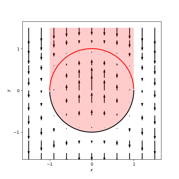
A. B.

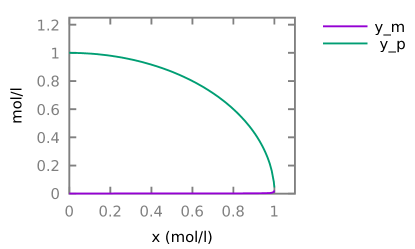
Figure 1: A. Flow diagram in the $x,y$ plane before the dual rail encoding for the stabilization of the unit circle. The arrows indicate the direction and strength of the flow. The upper part of the curve (in red) indicates the stable branch of the system and we colored in light red the domain ${\cal D}$ in which the system will reach the desired steady state. Outside of ${\cal D}$, the system is driven to the divergent state $\lim y=-\infty$. B. Dose response diagram of the generated CRN where the input concentration ($x$) is gradually increased from $0$ to $1$ while recording the steady state value of the output species $y^{+},y^{-}$.

Example 5

Even rather involved algebraic curves need surprisingly few species and reactions. This is the case of the serpentine curve, or anguinea, defined by the polynomial $(y-2)\left((x-10)^{2}+1\right)=4(x-10)$ for which we choose the point $x=10,y=2$ to enforce stability. The compilation process takes less than 100ms on a typical laptop. The generated CRN reproduces the anguinea curve on the $y$ variable, as shown in Fig.  2. It is composed of the following $4$ species and $12$ reactions:

$$\begin{aligned} y_{m}+y_{p}&\xrightarrow{\text{fast}}\emptyset,&\quad 2x&\rightarrow z+2x,\\ z&\rightarrow\emptyset,&\quad\emptyset&\xrightarrow{162}y_{p},\\ y_{m}&\xrightarrow{101}\emptyset,&\quad x+y_{p}&\xrightarrow{20}x+2y_{p},\\ z+y_{m}&\rightarrow z,&\quad z&\xrightarrow{2}z+y_{p},\\ x&\xrightarrow{36}x+y_{m},&\quad y_{p}&\xrightarrow{101}\emptyset,\\ x+y_{m}&\xrightarrow{20}x+2y_{m},&\quad z+y_{p}&\rightarrow z.\end{aligned}$$ (12)

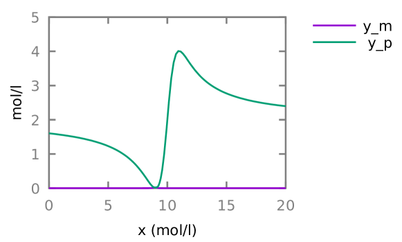
Figure 2: Dose-response diagram of the CRN generated by compilation of the serpentine algebraic curve, $(y-2)\left((x-10)^{2}+1\right)=4(x-10)$, with $x$ as input and $y$ as output.

Example 6

In the field of real analysis, the Bring radical of a real number $x$ is defined as the unique real root of the polynomial: $y^{5}+y+x$. The Bring radical is an algebraic function of $x$ that cannot be expressed by any algebraic expression.

The stabilizing CRN generated by our compilation pipeline is composed of $7$ species (${y_{m},y_{p},y2_{m},y2_{p},y3_{m},y3_{p},x}$) and $20$ reactions presented in model 13. A dose-response diagram of that CRN is shown in Fig. 3.

$$\begin{aligned} y_{m}+y_{p}&\xrightarrow{\text{fast}}\emptyset,&\quad y2_{m}+y2_{p}&\xrightarrow{\text{fast}}\emptyset,\\ y3_{m}+y3_{p}&\xrightarrow{\text{fast}}\emptyset,&\quad y_{p}&\xrightarrow{}\emptyset,\\ y2_{m}+y3_{p}&\xrightarrow{}y2_{m}+y3_{p}+y_{p},&\quad y2_{p}+y3_{m}&\xrightarrow{}y2_{p}+y3_{m}+y_{p},\\ x&\xrightarrow{}x+y_{m},&\quad y_{m}&\xrightarrow{}\emptyset,\\ y2_{p}+y3_{p}&\xrightarrow{}y2_{p}+y3_{p}+y_{m},&\quad y2_{m}+y3_{m}&\xrightarrow{}y2_{m}+y3_{m}+y_{m},\\ 2\cdot y_{p}&\xrightarrow{}y2_{p}+2\cdot y_{p},&\quad 2\cdot y_{m}&\xrightarrow{}y2_{p}+2\cdot y_{m},\\ y2_{p}&\xrightarrow{}\emptyset,&\quad y2_{m}&\xrightarrow{}\emptyset,\\ y2_{p}+y_{p}&\xrightarrow{}y2_{p}+y3_{p}+y_{p},&\quad y2_{m}+y_{m}&\xrightarrow{}y2_{m}+y3_{p}+y_{m},\\ y3_{p}&\xrightarrow{}\emptyset,&\quad y2_{p}+y_{m}&\xrightarrow{}y2_{p}+y3_{m}+y_{m},\\ y2_{m}+y_{p}&\xrightarrow{}y2_{m}+y3_{m}+y_{p},&\quad y3_{m}&\xrightarrow{}\emptyset.\end{aligned}$$ (13)

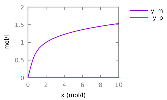
Figure 3: The bring radical is the real root of the polynomial equation $y^{5}+y+x=0$. As this quantity is negative, the output is read on the negative part of the output $y_{m}$. It is the simplest equation for which there is no expression for $y$ as a function of $x$.

Example 7

To generate the CRN that stabilize the Hill function of order 5, we can use the expression $y-\frac{x^{5}}{1+x^{5}}$ along with the point $x=1,y=\frac{1}{2}$. Our compilation pipeline generates the following model with $6$ species and $10$ reactions: $2x\rightarrow z_{1}+2x$, $2z_{1}\rightarrow z_{2}+2z_{1}$, $x+z_{2}\rightarrow x+z_{2}+z_{3}$, $\emptyset\rightarrow z_{4}$, $z_{4}+z_{3}\rightarrow z_{3}+y$, $z_{1}\rightarrow\emptyset$, $z_{2}\rightarrow\emptyset$, $z_{3}\rightarrow\emptyset$, $z_{4}\rightarrow\emptyset$, $y\rightarrow\emptyset$,
all kinetics being mass action law with unit rate. The $z^{\prime}s$ are auxiliary variables corresponding to the following expressions:

$$z_{1}=x^{2},\quad z_{2}=x^{4},\quad z_{3}=x^{5},\quad z_{4}=\frac{1}{1+x^{5}}.$$

The production and degradation of $z_{4}$ may be surprising, but looking at all the reactions implying both $z_{4}$ and $y$, we can see that their sum follow the equation $\frac{d(z_{4}+y)}{dt}=1-(z_{4}+y)$ hence ensuring that the sum of the two is fixed independently of their initial concentrations. It is worth remarking that another way of reaching the same result would be to directly build-in conservation laws into our CRN, hence using both steady state and invariant laws to define our steady state which however would make us sensitive to the initial concentrations.

6 Conclusion and Perspectives

We have introduced a notion of on-line analog computation for CRNs in which the concentration of one output species stabilizes to the result of some function of the concentrations of the input species, whatever perturbations are applied to the species concentrations during computation before the inputs stabilize. We have shown that the real functions that can be stably computed by a CRN in that way is precisely the set of real algebraic functions, defined by a polynomial and one point. Furthermore, we have derived from the constructive proof of this result a compilation pipeline to transform any algebraic function in a stabilizing CRN which computes it online.

These results open a whole research avenue for both the understanding of the structure of natural CRNs that allow cells to adapt to their environment, and for the design of artificial CRNs to implement high-level functions in chemistry. In the latter perspective of synthetic biology, our compilation pipeline makes it possible to automatically generate an abstract CRN which remains to be implemented with real enzymes, as in [8]. Taking into account a catalog of concrete enzymatic reactions earlier on in our compilation pipeline, in the polynomialization, quadratization and dual-rail encoding steps, is a particularly interesting, yet hard, challenge in order to guide search towards both concrete and economical solutions.

Our main theorem describes only CRNs at steady state only, while important aspects of signal processing are linked to the temporal evolution of the signals. Since our computation framework relies on ratios between production and degradation, a multiplication of both terms by some factor might be the matter of future work to control the characteristic time $\tau$ of equilibration, with high value of $\tau$ filtering out the high frequency noise of the inputs, and small $\tau$ values resulting in a more accurate output, yet at the expense of a higher protein turnover.

Acknowledgments.

We are grateful to Amaury Pouly and Sylvain Soliman for interesting discussions on this work, and to ANR-20-CE48-0002 and Inria AEx GRAM grants for partial support.

References

- [1] H. J. Buisman, H. M. M. ten Eikelder, P. A. J. Hilbers, and A. M. L. Liekens. Computing algebraic functions with biochemical reaction networks. Artificial Life, 15(1):5–19, 2009.
- [2] Laurence Calzone, François Fages, and Sylvain Soliman. BIOCHAM: An environment for modeling biological systems and formalizing experimental knowledge. Bioinformatics, 22(14):1805–1807, 2006.
- [3] Luca Cardelli, Mirco Tribastone, and Max Tschaikowski. From electric circuits to chemical networks. Natural Computing, 19, 2020.
- [4] David C. Carothers, G. Edgar Parker, James S. Sochacki, and Paul G. Warne. Some properties of solutions to polynomial systems of differential equations. Electronic Journal of Differential Equations, 2005(40):1–17, 2005.
- [5] Vijayalakshmi Chelliah, Camille Laibe, and Nicolas Novère. Biomodels database: A repository of mathematical models of biological processes. In Maria Victoria Schneider, editor, In Silico Systems Biology, volume 1021 of Methods in Molecular Biology, pages 189–199. Humana Press, 2013.
- [6] Ho-Lin Chen, David Doty, and David Soloveichik. Deterministic function computation with chemical reaction networks. Natural computing, 7433:25–42, 2012.
- [7] Matthew Cook, David Soloveichik, Erik Winfree, and Jehoshua Bruck. Programmability of chemical reaction networks. In Anne Condon, David Harel, Joost N. Kok, Arto Salomaa, and Erik Winfree, editors, Algorithmic Bioprocesses, pages 543–584. Springer Berlin Heidelberg, Berlin, Heidelberg, 2009.
- [8] Alexis Courbet, Patrick Amar, François Fages, Eric Renard, and Franck Molina. Computer-aided biochemical programming of synthetic microreactors as diagnostic devices. Molecular Systems Biology, 14(4), 2018.
- [9] Gheorghe Craciun and Martin Feinberg. Multiple equilibria in complex chemical reaction networks: II. the species-reaction graph. SIAM Journal on Applied Mathematics, 66(4):1321–1338, 2006.
- [10] X. Duportet, L. Wroblewska, P. Guye, Y. Li, J. Eyquem, J. Rieders, G. Batt, and R. Weiss. A platform for rapid prototyping of synthetic gene networks in mammalian cells. Nucleic Acids Research, 42(21), 2014.
- [11] Péter Érdi and János Tóth. Mathematical Models of Chemical Reactions: Theory and Applications of Deterministic and Stochastic Models. Nonlinear science : theory and applications. Manchester University Press, 1989.
- [12] François Fages, Guillaume Le Guludec, Olivier Bournez, and Amaury Pouly. Strong Turing Completeness of Continuous Chemical Reaction Networks and Compilation of Mixed Analog-Digital Programs. In CMSB’17: Proceedings of the fiveteen international conference on Computational Methods in Systems Biology, volume 10545 of Lecture Notes in Computer Science, pages 108–127. Springer-Verlag, September 2017.
- [13] François Fages, Steven Gay, and Sylvain Soliman. Inferring reaction systems from ordinary differential equations. Theoretical Computer Science, 599:64–78, September 2015.
- [14] François Fages and Sylvain Soliman. Abstract interpretation and types for systems biology. Theoretical Computer Science, 403(1):52–70, 2008.
- [15] Martin Feinberg. Mathematical aspects of mass action kinetics. In L. Lapidus and N. R. Amundson, editors, Chemical Reactor Theory: A Review, chapter 1, pages 1–78. Prentice-Hall, 1977.
- [16] Mathieu Hemery, François Fages, and Sylvain Soliman. On the complexity of quadratization for polynomial differential equations. In CMSB’20: Proceedings of the eighteenth international conference on Computational Methods in Systems Biology, Lecture Notes in BioInformatics. Springer-Verlag, September 2020.
- [17] Mathieu Hemery, François Fages, and Sylvain Soliman. Compiling elementary mathematical functions into finite chemical reaction networks via a polynomialization algorithm for ODEs. In CMSB’21: Proceedings of the nineteenth international conference on Computational Methods in Systems Biology, Lecture Notes in BioInformatics. Springer-Verlag, September 2021.
- [18] Chi-Ying Huang and James E. Ferrell. Ultrasensitivity in the mitogen-activated protein kinase cascade. PNAS, 93(19):10078–10083, September 1996.
- [19] Michael Hucka et al. The systems biology markup language (SBML): A medium for representation and exchange of biochemical network models. Bioinformatics, 19(4):524–531, 2003.
- [20] Lulu Qian, David Soloveichik, and Erik Winfree. Efficient turing-universal computation with DNA polymers. In Proc. DNA Computing and Molecular Programming, volume 6518 of LNCS, pages 123–140. Springer-Verlag, 2011.
- [21] Lee A. Segel. Modeling dynamic phenomena in molecular and cellular biology. Cambridge University Press, 1984.
- [22] Marko Vasic, David Soloveichik, and Sarfraz Khurshid. CRN++: Molecular programming language. In Proc. DNA Computing and Molecular Programming, volume 11145 of LNCS, pages 1–18. Springer-Verlag, 2018.