JT Gravity from Partial Reduction and Defect Extremal Surface

Abstract

We propose the three-dimensional bulk dual for Jackiw-Teitelboim gravity coupled with CFT₂ bath based on partial reduction. The bulk dual is classical AdS gravity with a defect brane which has small fluctuation in transverse direction. We derive full Jackiw-Teitelboim gravity action by considering the transverse fluctuation as a dilaton field. We demonstrate that the fine grained entropy computed from island formula precisely agrees with that computed from defect extremal surface. Our construction provides a Lorentzian higher dimensional dual for Jackiw-Teitelboim gravity and therefore offers a framework to study problems such as black hole information paradox as well as gravity/ensemble duality.

.1 Introduction

Significant progress has been made in recent understanding of black hole information paradox [1]. In particular the island formula [2, 3, 4] for the von Neumann entropy of Hawking radiation [5] gives Page curve [6] and therefore maintains unitarity. The development relies on the quantum extremal surface formula [7] for the fine grained entropy, which was based on the quantum corrected Ryu-Takayanagi formula in computing holographic entanglement entropy [8, 9, 10]. To justify the island formula of von Neumann entropy, one can employ replica trick and perform explicit gravitational path integral computation in lower dimensional systems. In particular the Jackiw-Teitelboim (JT) gravity coupled to a quantum bath provides a solvable model to explore the information transfer for black hole in two dimensions [11, 12]. It has been found that the island contribution corresponds to Euclidean replica wormholes [12], which may cause the factorization puzzle [13, 14]. It is still quite interesting to explore the Lorentzian counterparts for the replica wormholes. There are many applications and generalizations of island formula, including the application in cosmology [15, 16] and the generalization to asymptotically flat space [17, 18]. For other related works, see [19, 20, 21, 22, 23, 24, 25, 26, 27, 28, 29, 30, 31, 32, 33, 34, 35, 36, 37, 31, 38, 39, 40, 41, 42, 43]. On the other hand, AdS gravity with a defect brane provides a natural holographic framework to study lower dimensional gravity coupled to a bath. There the holographic dual of von Neumann entropy is Ryu-Takayangai surface or Hubeny-Rangamani-Takayanagi surface and therefore Lorentzian. The defect brane model can also be generalized to higher dimensions [44].

In [45], it has been shown that the holographic counterpart of island formula is Defect Extremal Surface (DES) formula, which is the defect corrected Ryu-Takayanagi formula. The defect brane model is based on $\text{AdS}_{\text{d+1}}/\text{BCFT}_{\text{d}}$ [46], where the defect brane with a constant tension in the AdS bulk has $\text{AdS}_{\text{d}}$ geometry and there are also quantum degrees of freedom localized on it. By doing partial dimension reduction between zero tension brane and constant tension brane, one can obtain the brane world gravity, which is coupled to a CFT bath through boundary conditions. In three dimensional bulk, the simple dimension reduction leads to a two dimensional topological gravity on the brane  [45]. It has been further demonstrated that entanglement entropy and reflected entropy computed from DES formula agrees with island formula precisely [47]. See [48, 49, 50, 51] for further works along this line. To fully reconcile the path integral approach and holographic approach, one may ask whether we can obtain JT gravity, which has a dilaton field, directly from dimension reduction in the defect brane model. If yes, what would be the holographic counterpart of the island formula for JT gravity coupled with CFT bath?

In this letter we answer these questions. We show that for the 3d AdS bulk with a defect brane, by considering the small transverse fluctuation, one can derive the full JT gravity action from partial reduction between zero tension brane and finite tension brane. In particular, the transverse fluctuation becomes the dilaton field on the brane world. For the remaining part of the bulk one can use standard AdS/CFT and obtain CFT₂ bath on the asymptotic boundary. Eventually we obtain a 2d JT gravity coupled with CFT₂ bath. The fact that the transverse fluctuation is small allows us to ignore higher order contributions in 2d action and obtain precisely the full 2d JT action including boundary term.We therefore obtain a higher dimensional dual for JT gravity coupled to a bath.

To support the 3d/2d duality, we compute the fined-grained entropy both from defect extremal surface formula in the bulk and from the boundary island formula. We find that the extremal conditions are consistent and the fined-grained entropy agree with each other precisely for small transverse fluctuation. We consider this agreement as strong evidence to support that JT gravity coupled to CFT bath can be dual to semi-classical 3d gravity with a fluctuating brane.

.2 Review of the model

We consider $\rm{AdS_{3}}/\rm{BCFT_{2}}$ with the action given by

$$\begin{split}I&=\frac{1}{16\pi G_{N}}\int_{N}\sqrt{-g}(R-2\Lambda)\\ &+\frac{1}{8\pi G_{N}}\int_{M}\sqrt{-\gamma}K^{(\gamma)}\\ &+\frac{1}{8\pi G_{N}}\int_{Q}\sqrt{-h}K^{(h)}\\ &+I_{Q}+I_{P}\ ,\end{split}$$ (1)

where $N$ denotes the bulk AdS spacetime, $M$ denotes the asymptotic boundary where the Dirichlet boundary condition is imposed and $Q$ the brane where Neumann boundary condition is imposed. $I_{Q}$ is the action for matter fields constrained on $Q$ and $I_{P}$ is the counter term on the tip $P$. By varying this action, the Neumann boundary condition on $Q$ becomes

$$K_{ab}^{(h)}-h_{ab}K^{(h)}=8\pi G_{N}T_{ab}\ ,$$ (2)

where $T_{ab}=-\frac{2}{\sqrt{-h}}\frac{\delta I_{Q}}{\delta h^{ab}}$ is the stress energy tensor coming from the variation of matter action.

Here we consider the bulk to be 3 dimensional and the brane $Q$ is thus two dimensional. There are two sets of useful coordinates: $(t,x,z)$ and $(t,\rho,y)$. Their relation is

$$z=-y/\cosh\frac{\rho}{l}\ ,\quad x=y\tanh\frac{\rho}{l}\,$$ (3)

and the bulk metric can be written in terms of either one

$$\begin{split}ds^{2}_{N}&=\frac{l^{2}}{z^{2}}(-dt^{2}+dz^{2}+dx^{2})\\ &=d\rho^{2}+l^{2}\cosh^{2}\frac{\rho}{l}\cdot\frac{-dt^{2}+dy^{2}}{y^{2}},\end{split}$$ (4)

where $l$ is the AdS radius. It is also useful to introduce polar coordinate $\theta$ with $\frac{1}{\cos(\theta)}=\cosh\left(\frac{\rho}{l}\right)$.

Consider the matter action on the brane $Q$ of the form

$$I_{Q}=-\frac{1}{8\pi G_{N}}\int_{Q}\sqrt{-h}T,$$ (5)

where $T$ is a constant tension. By solving (2), one can determine that the brane is located at $\rho=\rho_{0}=\text{arctanh}\sin\theta_{0}$, where $\rho_{0}$ is a positive constant. See FIG. 1 for an illustration.

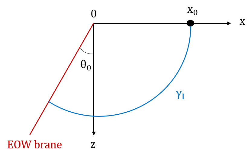
Figure 1: The set up of AdS/BCFT where the brane tension is a constant.

The tension $T$ is found to be

$$T=\frac{\tanh\frac{\rho_{0}}{l}}{l}.$$ (6)

For an interval $I:=[0,x_{0}]$ in BCFT, the entanglement entropy can be computed holographically using RT formula. As shown in FIG.1, the minimal surface denoted by $\gamma_{I}$ terminates on a point on the brane which can be determined by extremization. The entanglement entropy is

$$\begin{split}S_{I}&=\frac{\operatorname{Area}\left(\gamma_{I}\right)}{4G_{N}}=\frac{c}{6}\log\frac{2x_{0}}{\epsilon}+\frac{c}{6}\rho_{0}\\ &=\frac{c}{6}\log\frac{2x_{0}}{\epsilon}+\frac{c}{6}\operatorname{arctanh}(\sin\theta_{0}),\end{split}$$ (7)

where $c$ is the CFT central charge and $\epsilon$ is the UV cut off.

In [45], the authors improved AdS₃/CFT₂ by adding CFT matter localized on the brane. Notice that ${\rm{AdS}}_{2}$ is a maximally symmetric space, the vacuum one point function of the CFT stress tensor takes the form

$$\langle T_{ab}\rangle_{\text{AdS}_{2}}=\chi h_{ab}\ ,$$ (8)

which contributes to Neumann boundary condition (2). Because of the entangled quantum matter on the defect brane, we should add the defect contribution to the ordinary holographic entanglement entropy. The improved holographic formula is therefore called Defect Extremal Surface (DES) formula [45].

.3 JT gravity from dimensional reduction

Now we derive JT gravity from dimension reduction of 3d AdS gravity action. Under the metric ansatz

$$ds^{2}=g_{\mu\nu}dx^{\mu}dx^{\nu}=d\rho^{2}+l^{2}\cosh^{2}\frac{\rho}{l}{\tilde{h}}_{ab}dx^{a}dx^{b},$$ (9)

one can perform partial dimensional reduction for wedge $W_{1}+\tilde{W}$ by integrating out the $\rho$ direction as shown in FIG. 2. The bulk action becomes

$$\begin{split}&\frac{1}{16\pi G_{N}}\int_{W_{1}+\tilde{W}}\sqrt{-g}(R-2\Lambda)\\ &=\int\frac{\rho_{0}+\tilde{\rho}}{16\pi G_{N}}\sqrt{-g^{(2)}}R^{(2)}\\ &-\int\frac{1}{16\pi G_{N}}\frac{\sinh(\frac{2\rho}{l})}{l\cosh^{2}\frac{\rho_{0}}{l}}\sqrt{-g^{(2)}},\end{split}$$ (10)

where $\Lambda=-\frac{2}{l^{2}}$ and

$$g_{ab}^{(2)}=l^{2}{\rm{cosh}}^{2}\frac{\rho_{0}}{l}{\tilde{h}}_{ab}.$$ (11)

The precise reduction of bulk Ricci scalar

$$\sqrt{-g}R=\sqrt{-g^{(2)}}\left[R^{(2)}-\frac{2(3\cosh^{2}\frac{\rho}{l}-1)}{l^{2}\cosh^{2}\frac{\rho_{0}}{l}}\right]$$ (12)

has been used in eq.(LABEL:EH2). Notice that the brane $Q$ is located at

$$\rho=\rho_{0}+\tilde{\rho},$$ (13)

where $\tilde{\rho}$ is a small fluctuation away from $\rho_{0}$, i.e.$\frac{\tilde{\rho}}{\rho_{0}}\ll 1$. The fluctuation $\tilde{\rho}$ is a function of the brane world coordinates and therefore should be treated as a field on the brane.

Next we consider Gibbons-Hawking term and the brane tension term. The extrinsic curvature of the brane is

$$K_{ab}=\frac{\tanh(\frac{\rho_{0}+\tilde{\rho}}{l})}{l}{h}_{ab},$$ (14)

where ${h}_{ab}$ is the induced metric on the brane

$${h}_{ab}=l^{2}{\rm{cosh}}^{2}\frac{\rho}{l}\tilde{h}_{ab}.$$ (15)

The tension of the brane remains a constant which equals to the tension (6) since the fluctuation of the $\rho$ coordinate will not affect the intrinsic brane tension. Then Gibbons-Hawking term plus the brane tension term is given by

$$\begin{split}&\frac{1}{8\pi G_{N}}\int_{Q}\sqrt{-{h}}(K-T)\\ &=\frac{1}{8\pi G_{N}}\int\frac{\sinh(\frac{2\rho_{0}+2\tilde{\rho}}{l})}{l\cosh^{2}\frac{\rho_{0}}{l}}\sqrt{-g^{(2)}}\\ &-\frac{1}{8\pi G_{N}}\int\frac{\tanh\frac{\rho_{0}}{l}\cosh^{2}(\frac{\rho_{0}+\tilde{\rho}}{l})}{l\cosh^{2}\frac{\rho_{0}}{l}}\sqrt{-g^{(2)}}.\end{split}$$ (16)

By adding (LABEL:EH2) and (LABEL:GH) together and expanding with small $\tilde{\rho}/\rho_{0}$, we get the action of the 2d effective theory after partial dimension reduction

$$\begin{split}I_{tot}&=\frac{\rho_{0}}{16\pi G_{N}}\int\sqrt{-g^{(2)}}\frac{\tilde{\rho}}{\rho_{0}}\left(R^{(2)}+\frac{2}{l^{2}\cosh^{2}\frac{\rho_{0}}{l}}\right)\\ &+\frac{\rho_{0}}{16\pi G_{N}}\int\sqrt{-g^{(2)}}R^{(2)}+\mathcal{O}(\frac{\tilde{\rho}^{2}}{{\rho_{0}}^{2}}).\end{split}$$ (17)

Neglecting $\mathcal{O}(\frac{\tilde{\rho}^{2}}{{\rho_{0}}^{2}})$ terms, we see that the action is precisely the JT action, and $\frac{\tilde{\rho}}{\rho_{0}}$ is identified as the dilaton field in JT gravity. If we vary with respect to $\frac{\tilde{\rho}}{\rho_{0}}$, we get the scalar curvature

$$R^{(2)}=-\frac{2}{l^{2}\cosh^{2}\frac{\rho_{0}}{l}},$$ (18)

which gives the correct scalar curvature of the ${\rm{AdS}}_{2}$ brane world.

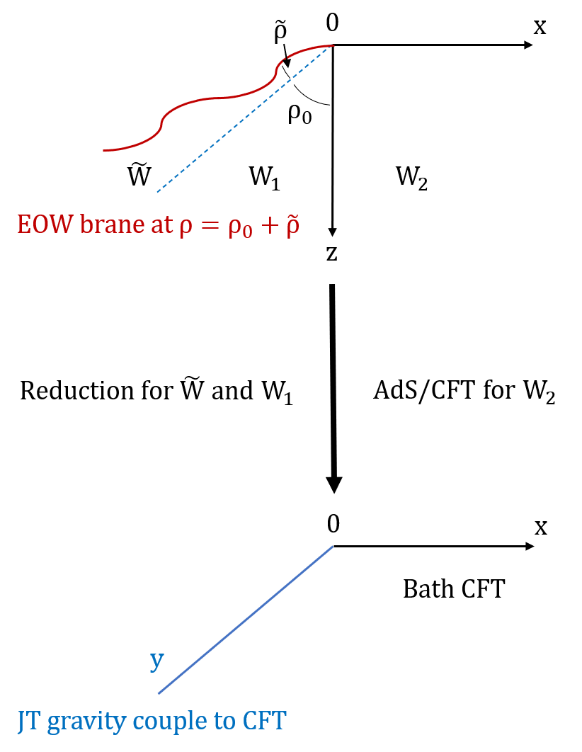
Figure 2: Effective description from Partial Dimension Reduction plus AdS/CFT.

To fully recover the JT action, we also need to reproduce the boundary term. Now we show that the JT boundary action can be obtained by doing dimension reduction from the Gibbons-Hawking term on the bulk cutoff surface. . As shown in FIG. 3, the cutoff surface is denoted as $\Sigma$. Near the asymptotic boundary, the metric is taken to be

$$ds^{2}=d\rho^{2}+l^{2}\cosh^{2}\frac{\rho}{l}\frac{-dt^{2}+dy^{2}}{y^{2}}.$$ (19)

Consider a generic cutoff surface $\Sigma$ parameterized by

$$(y,t)=(y(u),t(u)),$$ (20)

where $u$ is the time in the cutoff boundary. The induced metric at cutoff surface is

$$ds^{2}=d\rho^{2}+l^{2}\cosh^{2}(\frac{\rho}{l})(\frac{y^{\prime 2}du^{2}-t^{\prime 2}du^{2}}{y^{2}})$$ (21)

where we denote $y^{\prime}=\frac{dy}{du}$, $t^{\prime}=\frac{dt}{du}$. One can compute the extrinsic curvature of $\Sigma$ by $K=g^{\mu\nu}\nabla_{\mu}n_{\nu}$ and the result is

$$K_{\Sigma}=\frac{1}{l\cosh\frac{\rho}{l}}\frac{t^{\prime 3}+yy^{\prime}t^{\prime\prime}-t^{\prime}y^{\prime 2}-t^{\prime}yy^{\prime\prime}}{(t^{\prime 2}-y^{\prime 2})^{3/2}}=\frac{1}{l\cosh\frac{\rho}{l}}K_{\Omega}$$ (22)

where $K_{\Omega}=\frac{t^{\prime 3}+yy^{\prime}t^{\prime\prime}-t^{\prime}y^{\prime 2}-t^{\prime}yy^{\prime\prime}}{(t^{\prime 2}-y^{\prime 2})^{3/2}}$ is the extrinsic curvature of the boundary $\Omega$ which is the intersection between $\Sigma$ and EOW brane. By doing dimension reduction of Gibbons-Hawking term on $\Sigma$, the action on $\Omega$ is obtained

$$\begin{split}I_{bJT}&=\frac{1}{8\pi G_{N}}\int_{\Sigma}\sqrt{-\gamma}K_{\Sigma}\\ &=\frac{\rho_{0}}{8\pi G_{N}}\int du\sqrt{\frac{t^{\prime 2}-y^{\prime 2}}{y^{2}}}(1+\frac{\tilde{\rho}}{\rho_{0}}|_{\mathrm{bdy}})K_{\Omega},\end{split}$$ (23)

This is precisely the boundary term of JT gravity when $\frac{\tilde{\rho}}{\rho_{0}}$ is identified as the dilaton field. At the intersection $\Omega$, employing the same trick in [53] one can fix the induced metric

$$g|_{\mathrm{bdy}}=-\frac{l^{2}\cosh^{2}(\frac{\rho}{l})}{\epsilon^{2}}.$$ (24)

By identifying the induced metric in (21) to (24), $y$ can be solved to the leading order in $\epsilon$, $y=\epsilon t^{\prime}+O(\epsilon^{2})$. By computing $K_{\Omega}$ directly, we find

$$K_{\Omega}=1-\epsilon^{2}{\rm{Sch}}(t(u),u).$$ (25)

If we neglect the field independent divergent term, the boundary term is a Schwarzian . We leave the computation details to appendix A.

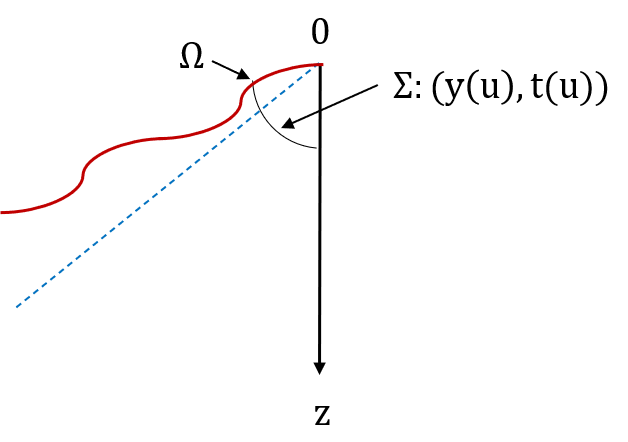
Figure 3: Dynamical UV cut off for the wedge $W_{1}+\tilde{W}$.

Thus after doing the partial dimension reduction for wedge $W_{1}+\tilde{W}$ and using standard AdS/CFT for wedge $W_{2}$, we obtain the 2d effective theory to be a JT gravity together with the brane CFT, glued to a non-gravitational CFT bath through transparent boundary conditions, which is precisely the original set up to motivate the island formula. See FIG. 2 for an illustration of this procedure.

.4 Entanglement entropy for an interval

.4.1 Entanglement entropy from island formula

Since we have obtained the 2d effective description in terms of a JT gravity glued with a CFT bath, we can use island formula to calculate the von Neumann entropy for an interval $[0,L]$ on the asymptotic boundary

$$S=\min_{X}\left\{\operatorname{ext}_{X}\left[\frac{\operatorname{Area}(X)}{4G_{N}}+S_{\text{semi-cl }}\left(\Sigma_{X}\right)\right]\right\},$$ (26)

where $X=\partial I$ and $I$ is the island, $\Sigma_{X}$ is the associated region including the island and $S_{\rm{semi-cl}}(\Sigma_{X})$ is the von-Neumann entropy of the quantum fields on $\Sigma_{X}$ in the semi-classical description. Introducing the 2d Newton constant

$$G_{N}^{(2)}=\frac{G_{N}}{\rho_{0}},$$ (27)

the action of 2d effective theory becomes

$$\begin{split}I_{\text{2d}}&=\frac{1}{16\pi G_{N}^{(2)}}\int\sqrt{-g^{(2)}}R^{(2)}\\ &+\frac{1}{16\pi G_{N}^{(2)}}\int\sqrt{-g^{(2)}}\frac{\tilde{\rho}}{\rho_{0}}\left(R^{(2)}+\frac{2}{l^{2}\cosh^{2}\frac{\rho_{0}}{l}}\right)\\ &+I_{\text{CFT}}.\end{split}$$ (28)

Varying with respect to the 2d metric one can solve the dilaton to be

$$\frac{\tilde{\rho}}{\rho_{0}}=-\frac{\bar{\phi}_{r}}{y}.$$ (29)

Now we employ island formula to calculate the entropy of a single interval $[0,L]$. For simplicity we focus on static cases. The generalized entropy is given by

$$S_{\text{gen}}(a) =S_{\text{area }}(y=-a)+S_{\text{matter }}([-a,L])$$ (30)

$$=\frac{1}{4G_{N}^{(2)}}(1+\frac{\tilde{\rho}}{\rho_{0}})+\frac{c}{6}\log\frac{(L+a)^{2}l}{a\cos\theta_{0}\epsilon\epsilon_{y}}.$$

The extremization condition $\partial_{a}S_{\text{gen}}(a)=0$ determines the boundary of island $a$ to be

$$a=\frac{L}{2}\left(\sqrt{36\mu^{2}+36\mu+1}+6\mu+1\right),$$ (31)

where $\mu$ is defined as $\mu=\frac{\rho_{0}\bar{\phi}_{r}}{6lL}$, which can also be expressed as $\frac{1}{6}\cdot\frac{\tilde{\rho}(a)}{l}\cdot\frac{a}{L}$ because of eq.(29). It characterizes the amplitude of the brane transverse fluctuation at location $a$, since $\frac{a}{L}$ measures the distance from the origin and $\frac{\tilde{\rho}}{l}$ measures the fluctuation in angular direction. In fact one can work out a simple relation between extremal point $a$ and $\tilde{\rho}(a)$

$$\frac{a}{L}=\frac{1+\frac{\tilde{\rho}(a)}{l}}{1-\frac{\tilde{\rho}(a)}{l}}.$$ (32)

By plugging (31) into $S_{\text{gen}}(a)$ one can get the entropy $S_{\text{island}}$ computed from island formula.

.4.2 Entanglement entropy from bulk DES

The defect extremal surface formula is the defect corrected Ryu-Takayanagi formula. For defect $D$ in the AdS bulk, the entanglement entropy is computed following

$$\begin{split}S_{\mathrm{DES}}&=\min_{\Gamma}\left\{\operatorname{ext}_{\Gamma,X}\left[\frac{\operatorname{Area}(\Gamma)}{4G_{N}}+S_{\mathrm{defect}}[D]\right]\right\},\end{split}$$ (33)

where $X=\Gamma\cap D$ and $\Gamma$ is the codimension two RT surface. We consider the interval $[0,L]$ on the asymptotic boundary and use DES formula to calculate its entropy. First we compute the RT surface $\frac{\operatorname{Area}(\Gamma)}{4G_{N}}$ by using embedding coordinates. Considering $\frac{\tilde{\rho}}{\rho_{0}}\ll 1$, the leading order result is

$$\begin{split}\frac{\text{Area}(\Gamma)}{4G_{N}}&=\frac{l}{4G_{N}}\operatorname{arccosh}\left[\frac{(L+a\sin\theta_{0})^{2}+a^{2}\cos^{2}\theta_{0}}{2a\cos\theta_{0}\epsilon}\right]\\ &+\frac{\rho_{0}\bar{\phi}_{r}}{4G_{N}a}.\end{split}$$ (34)

We leave the details to appendix B. The brane CFT also contributes to the entanglement entropy

$$S_{\text{defect}}(D)=\frac{c^{\prime}}{6}\log\frac{2l}{\epsilon_{y}\cos\theta_{0}}.$$ (35)

Then the total generalized entropy is

$$\begin{split}S_{\text{gen}}(a)&=\frac{c}{6}\operatorname{log}\left[\frac{(L+a\sin\theta_{0})^{2}+a^{2}\cos^{2}\theta_{0}}{a\cos\theta_{0}\epsilon}\right]\\ &+\frac{\rho_{0}\bar{\phi}_{r}}{4G_{N}a}+\frac{c^{\prime}}{6}\log\frac{2l}{\epsilon_{y}\cos\theta_{0}},\end{split}$$ (36)

where $c=\frac{3l}{2G_{N}}$ is used and $c^{\prime}$ is the central charge of the brane CFT. To compare with the result obtained from boundary island formula, we take $c^{\prime}=c$.

From $\partial_{a}S_{gen}(a)=0$, one obtains the extremal position of $a$ to be

$$a =\frac{(3)^{\frac{2}{3}}L\left(12\mu^{2}+12\mu\sin\theta_{0}+1\right)}{3\nu}$$ (37)

$$+2\mu L+\frac{L\nu}{3^{\frac{2}{3}}},$$

where

$$\begin{split}\nu&=\sqrt[3]{72\mu^{3}+\frac{1}{6}\sqrt{\gamma}+108\mu^{2}\sin\theta_{0}+36\mu}\\ \gamma&=46656\mu^{2}\left(2\mu^{2}+3\mu\sin\theta_{0}+1\right)^{2}\\ &-108\left(12\mu^{2}+12\mu\sin\theta_{0}+1\right)^{3}.\end{split}$$ (38)

Plugging (37) into $S_{\text{gen}}(a)$, we have the entropy result calculated from DES.

.4.3 Comparison between DES and island formula

Now we compare the entropy result computed from DES and that from island formula.

We first consider $\rho_{0}/l\gg 1$ with the small fluctuation condition $\tilde{\rho}/\rho_{0}\ll 1$ satisfied. This is the limit that the brane is nearly parallel to the asymptotic boundary. In this limit, the extremal point (31) and (37) coincide with each other and both DES and island formula give the same entropy. To see this, let us fix $\mu$ and set $\theta_{0}=\frac{\pi}{2}-\omega$ . Expanding the extremal point and the entropy around $\omega=0$, we get

$$\begin{split}a_{\text{DES}}&=\frac{L}{2}\left(\sqrt{36\mu^{2}+36\mu+1}+6\mu+1\right)+\mathcal{O}(\omega^{2})\\ &=a_{\text{island}}+\mathcal{O}(\omega^{2}),\end{split}$$ (39)

and

$$\begin{split}S_{\text{DES}}&=\frac{2c\mu}{6\mu+1+\eta}+\frac{c}{6}\log\frac{(6\mu+3+\eta)^{2}L}{(6\mu+1+\eta)\epsilon}\\ &+\frac{c}{6}\log\frac{l}{\omega^{2}\epsilon_{y}}+\mathcal{O}(\omega^{2})\\ &=S_{\text{island}}+\mathcal{O}(\omega^{2}),\end{split}$$ (40)

where

$$\eta=\sqrt{36\mu^{2}+36\mu+1}.$$ (41)

Furthermore, we can consider a generic brane location, i.e. $\rho_{0}/l$ is finite. By the small fluctuation condition $\frac{\tilde{\rho}}{\rho_{0}}\ll 1$, we have that $\tilde{\rho}/l$ is small, which implies that $\mu=\frac{1}{6}\cdot\frac{\tilde{\rho}}{l}\cdot\frac{a}{L}\ll 1$ provided that $a/L$ is order one. In this limit we can expand with small $\mu$. The extremal point of bulk DES becomes

$$a=L+6(1+\sin\theta_{0})L\mu+\mathcal{O}(\mu^{2}),$$ (42)

and the extremal point of island formula is

$$a=L+12L\mu+\mathcal{O}(\mu^{2}).$$ (43)

The entropy from bulk DES is

$$\begin{split}S_{\text{DES}}&=\frac{c}{6}\log\frac{2L}{\epsilon}+\frac{c}{6}\log\frac{1+\sin\theta_{0}}{\cos\theta_{0}}\\ &+\frac{c}{6}\log\frac{2l}{\epsilon_{y}\cos\theta_{0}}+c\mu+\mathcal{O}(\mu^{2}),\end{split}$$ (44)

while the entropy from boundary island formula is

$$\begin{split}S_{\text{island}}&=\frac{c}{6}\log\frac{2L}{\epsilon}+\frac{c}{6}\operatorname{arctanh}(\sin\theta_{0})\\ &+\frac{c}{6}\log\frac{2l}{\epsilon_{y}\cos\theta_{0}}+c\mu+\mathcal{O}(\mu^{2}).\end{split}$$ (45)

Comparing the above two results, we find that the entanglement entropy for single interval $[0,L]$ from DES and from island formula precisely match for small brane fluctuations.

.5 Conclusion and Discussion

In this paper we constructed the three-dimensional bulk dual for Jackiw-Teitelboim gravity coupled to CFT₂ bath based on partial reduction. The bulk dual is classical AdS gravity with a defect brane which has small fluctuation in transverse direction. We obtain full Jackiw-Teitelboim gravity action by identifying the transverse fluctuation as a dilaton field on brane world. We further demonstrated that the fine grained entropy computed from island formula precisely agrees with that computed from defect extremal surface. There are a few interesting future questions: First, using our construction to understand JT gravity/ensemble relation. In our construction the JT gravity from partial reduction is dual to a defect theory in asymptotic boundary and it would be interesting to check the relation between this defect theory and the ensemble of quantum mechanics discussed in [56]. Second, generalize our construction to higher dimensions. In higher dimensions, the dilaton field is known as radion field in the original Randall-Sundrum model [57]. It is quite interesting to work out the full brane world theory including the dilaton field from partial reduction. Last but not least, it is interesting to test our construction by other entanglement measures and to explore the physical implications of the dilaton in brane world cosmology [49].

Note added: After this work is finished, [58] appears in arXiv, where the authors consider wedge holography with two finite tension branes.

Appendix A Schwarzian theory on the JT boundary

In this appendix we show further details of how to compute the JT boundary term and recognize that this is a Schwarzian theory.

We consider the UV cutoff surface $\Sigma$, the tangent vector and normal vector are

$$T^{\nu}=\frac{1}{l\cosh(\frac{\rho}{l})}(t^{\prime},y^{\prime},0),$$ (46)

$$n_{\mu}=(\frac{y^{\prime}l\cosh\frac{\rho}{l}}{y\sqrt{t^{\prime 2}-y^{\prime 2}}},-\frac{t^{\prime}l\cosh\frac{\rho}{l}}{y\sqrt{t^{\prime 2}-y^{\prime 2}}},0).$$ (47)

The extrinsic curvature is computed as

$$\begin{split}K&=g^{\mu\nu}\nabla_{\mu}n_{\nu}\\ &=-\frac{T^{\nu}}{T^{2}}\nabla_{T}n_{\nu}=-\frac{T^{\nu}}{T^{2}}(\partial_{u}n_{\nu}-\Gamma^{\rho}_{\mu\nu}n_{\rho}T^{\mu})\\ &=\frac{1}{l\cosh\frac{\rho}{l}}\frac{t^{\prime 3}+yy^{\prime}t^{\prime\prime}-t^{\prime}y^{\prime 2}-t^{\prime}yy^{\prime\prime}}{(t^{\prime 2}-y^{\prime 2})^{3/2}}\end{split}$$ (48)

By using $y=\epsilon t^{\prime}$ and expand $K$ to $O(\epsilon^{2})$, we get

$$K=\frac{1}{l\cosh{\frac{\rho}{l}}}(1-\epsilon^{2}{\rm{Sch}}(t(u),u))$$ (49)

Where

$${\rm{Sch}}(t(u),u)=\frac{2t^{\prime}t^{\prime\prime\prime}-3t^{\prime\prime 2}}{2t^{\prime 2}}.$$ (50)

Appendix B Computation of bulk RT surface contribution

In this appendix, we compute the entropy contribution of RT surface by using embedding coordinates.

The embedding coordinates are

$$\begin{split}X^{0}&=\frac{z}{2}+\frac{1}{2z}\left(\ell^{2}+x^{2}-t^{2}\right),\\ X^{1}&=\frac{\ell^{2}}{z}t,\\ X^{2}&=\frac{\ell^{2}}{z}x,\\ X^{3}&=\frac{z}{2}-\frac{1}{2z}\left(\ell^{2}-x^{2}+t^{2}\right),\end{split}$$ (51)

where $\left(X^{0}\right)^{2}+\left(X^{1}\right)^{2}-\left(X^{2}\right)^{2}-\left(X^{3}\right)^{2}=\ell^{2}$. Using these the geodesic distance $s$ between two points $\left(t_{1},z_{1},x_{1}\right)$ and $\left(t_{2},z_{2},x_{2}\right)$ is obtained as

$$s=l\operatorname{arccosh}\left[\frac{-\left(t_{2}-t_{1}\right)^{2}+\left(x_{2}-x_{1}\right)^{2}+z_{1}^{2}+z_{2}^{2}}{2z_{1}z_{2}}\right].$$ (52)

Plugging in two points $\text{A}=(t,a\cos\theta,-a\sin\theta)$ and $\text{B}=(t,\epsilon,L)$ where A is the intersection point of DES and EOW brane and B is the right boundary of the interval, one gets

$$\begin{split}\frac{\operatorname{Area}(\Gamma)}{4G_{N}}&=\frac{l}{4G_{N}}\operatorname{arccosh}\left[\frac{(L+a\sin\theta)^{2}+a^{2}\cos^{2}\theta}{2a\cos\theta\epsilon}\right].\end{split}$$ (53)

Considering $\frac{\tilde{\rho}}{\rho_{0}}\ll 1$ , we can expand the RT result to the first order

$$\begin{split}\frac{\text{Area}(\Gamma)}{4G_{N}}&=\frac{l}{4G_{N}}\operatorname{arccosh}\left[\frac{(L+a\sin\theta_{0})^{2}+a^{2}\cos^{2}\theta_{0}}{2a\cos\theta_{0}\epsilon}\right]\\ &+\frac{\rho_{0}\bar{\phi}_{r}}{4G_{N}a},\end{split}$$ (54)

where $\frac{1}{\cos\theta}=\cosh(\frac{\rho_{0}+\tilde{\rho}}{l})$ and the solution (29) is used.

References

- Hawking [1976] S. W. Hawking, Breakdown of Predictability in Gravitational Collapse, Phys. Rev. D 14, 2460 (1976).
- Penington [2020] G. Penington, Entanglement Wedge Reconstruction and the Information Paradox, JHEP 09, 002, arXiv:1905.08255 [hep-th] .
- Almheiri et al. [2019] A. Almheiri, N. Engelhardt, D. Marolf, and H. Maxfield, The entropy of bulk quantum fields and the entanglement wedge of an evaporating black hole, JHEP 12, 063, arXiv:1905.08762 [hep-th] .
- Almheiri et al. [2020a] A. Almheiri, R. Mahajan, J. Maldacena, and Y. Zhao, The Page curve of Hawking radiation from semiclassical geometry, JHEP 03, 149, arXiv:1908.10996 [hep-th] .
- Hawking [1975] S. W. Hawking, Particle Creation by Black Holes, Commun. Math. Phys. 43, 199 (1975), [Erratum: Commun.Math.Phys. 46, 206 (1976)].
- Page [1993] D. N. Page, Information in black hole radiation, Phys. Rev. Lett. 71, 3743 (1993), arXiv:hep-th/9306083 .
- Engelhardt and Wall [2015] N. Engelhardt and A. C. Wall, Quantum Extremal Surfaces: Holographic Entanglement Entropy beyond the Classical Regime, JHEP 01, 073, arXiv:1408.3203 [hep-th] .
- Ryu and Takayanagi [2006] S. Ryu and T. Takayanagi, Holographic derivation of entanglement entropy from AdS/CFT, Phys. Rev. Lett. 96, 181602 (2006), arXiv:hep-th/0603001 .
- Hubeny et al. [2007] V. E. Hubeny, M. Rangamani, and T. Takayanagi, A Covariant holographic entanglement entropy proposal, JHEP 07, 062, arXiv:0705.0016 [hep-th] .
- Faulkner et al. [2013] T. Faulkner, A. Lewkowycz, and J. Maldacena, Quantum corrections to holographic entanglement entropy, JHEP 11, 074, arXiv:1307.2892 [hep-th] .
- Almheiri et al. [2020b] A. Almheiri, T. Hartman, J. Maldacena, E. Shaghoulian, and A. Tajdini, Replica Wormholes and the Entropy of Hawking Radiation, JHEP 05, 013, arXiv:1911.12333 [hep-th] .
- Penington et al. [2022] G. Penington, S. H. Shenker, D. Stanford, and Z. Yang, Replica wormholes and the black hole interior, JHEP 03, 205, arXiv:1911.11977 [hep-th] .
- Witten and Yau [1999] E. Witten and S.-T. Yau, Connectedness of the boundary in the AdS / CFT correspondence, Adv. Theor. Math. Phys. 3, 1635 (1999), arXiv:hep-th/9910245 .
- Maldacena and Maoz [2004] J. M. Maldacena and L. Maoz, Wormholes in AdS, JHEP 02, 053, arXiv:hep-th/0401024 .
- Chen et al. [2021a] Y. Chen, V. Gorbenko, and J. Maldacena, Bra-ket wormholes in gravitationally prepared states, JHEP 02, 009, arXiv:2007.16091 [hep-th] .
- Hartman et al. [2020a] T. Hartman, Y. Jiang, and E. Shaghoulian, Islands in cosmology, JHEP 11, 111, arXiv:2008.01022 [hep-th] .
- Hartman et al. [2020b] T. Hartman, E. Shaghoulian, and A. Strominger, Islands in Asymptotically Flat 2D Gravity, JHEP 07, 022, arXiv:2004.13857 [hep-th] .
- Krishnan et al. [2020] C. Krishnan, V. Patil, and J. Pereira, Page Curve and the Information Paradox in Flat Space, (2020), arXiv:2005.02993 [hep-th] .
- Chen [2020] Y. Chen, Pulling Out the Island with Modular Flow, JHEP 03, 033, arXiv:1912.02210 [hep-th] .
- Chen et al. [2020a] Y. Chen, X.-L. Qi, and P. Zhang, Replica wormhole and information retrieval in the SYK model coupled to Majorana chains, JHEP 06, 121, arXiv:2003.13147 [hep-th] .
- Sully et al. [2021] J. Sully, M. V. Raamsdonk, and D. Wakeham, BCFT entanglement entropy at large central charge and the black hole interior, JHEP 03, 167, arXiv:2004.13088 [hep-th] .
- Hollowood and Kumar [2020] T. J. Hollowood and S. P. Kumar, Islands and Page Curves for Evaporating Black Holes in JT Gravity, JHEP 08, 094, arXiv:2004.14944 [hep-th] .
- Geng and Karch [2020] H. Geng and A. Karch, Massive islands, JHEP 09, 121, arXiv:2006.02438 [hep-th] .
- Chen et al. [2020b] H. Z. Chen, Z. Fisher, J. Hernandez, R. C. Myers, and S.-M. Ruan, Information Flow in Black Hole Evaporation, JHEP 03, 152, arXiv:1911.03402 [hep-th] .
- Li et al. [2020] T. Li, J. Chu, and Y. Zhou, Reflected Entropy for an Evaporating Black Hole, JHEP 11, 155, arXiv:2006.10846 [hep-th] .
- Chandrasekaran et al. [2020] V. Chandrasekaran, M. Miyaji, and P. Rath, Including contributions from entanglement islands to the reflected entropy, Phys. Rev. D 102, 086009 (2020), arXiv:2006.10754 [hep-th] .
- Dong et al. [2020] X. Dong, X.-L. Qi, Z. Shangnan, and Z. Yang, Effective entropy of quantum fields coupled with gravity, JHEP 10, 052, arXiv:2007.02987 [hep-th] .
- Chen et al. [2021b] H. Z. Chen, Z. Fisher, J. Hernandez, R. C. Myers, and S.-M. Ruan, Evaporating Black Holes Coupled to a Thermal Bath, JHEP 01, 065, arXiv:2007.11658 [hep-th] .
- Balasubramanian et al. [2021] V. Balasubramanian, A. Kar, and T. Ugajin, Islands in de Sitter space, JHEP 02, 072, arXiv:2008.05275 [hep-th] .
- Chen et al. [2020c] H. Z. Chen, R. C. Myers, D. Neuenfeld, I. A. Reyes, and J. Sandor, Quantum Extremal Islands Made Easy, Part I: Entanglement on the Brane, JHEP 10, 166, arXiv:2006.04851 [hep-th] .
- Chen et al. [2020d] H. Z. Chen, R. C. Myers, D. Neuenfeld, I. A. Reyes, and J. Sandor, Quantum Extremal Islands Made Easy, Part II: Black Holes on the Brane, JHEP 12, 025, arXiv:2010.00018 [hep-th] .
- Ling et al. [2021] Y. Ling, Y. Liu, and Z.-Y. Xian, Island in Charged Black Holes, JHEP 03, 251, arXiv:2010.00037 [hep-th] .
- Harlow and Shaghoulian [2021] D. Harlow and E. Shaghoulian, Global symmetry, Euclidean gravity, and the black hole information problem, JHEP 04, 175, arXiv:2010.10539 [hep-th] .
- Hernandez et al. [2021] J. Hernandez, R. C. Myers, and S.-M. Ruan, Quantum extremal islands made easy. Part III. Complexity on the brane, JHEP 02, 173, arXiv:2010.16398 [hep-th] .
- Chen and Lin [2021] Y. Chen and H. W. Lin, Signatures of global symmetry violation in relative entropies and replica wormholes, JHEP 03, 040, arXiv:2011.06005 [hep-th] .
- Akal et al. [2020] I. Akal, Y. Kusuki, T. Takayanagi, and Z. Wei, Codimension two holography for wedges, Phys. Rev. D 102, 126007 (2020), arXiv:2007.06800 [hep-th] .
- Rozali et al. [2020] M. Rozali, J. Sully, M. Van Raamsdonk, C. Waddell, and D. Wakeham, Information radiation in BCFT models of black holes, JHEP 05, 004, arXiv:1910.12836 [hep-th] .
- Suzuki and Takayanagi [2022] K. Suzuki and T. Takayanagi, BCFT and Islands in Two Dimensions, (2022), arXiv:2202.08462 [hep-th] .
- Bousso and Wildenhain [2022] R. Bousso and E. Wildenhain, Islands in closed and open universes, Phys. Rev. D 105, 086012 (2022), arXiv:2202.05278 [hep-th] .
- Miyaji [2021] M. Miyaji, Island for gravitationally prepared state and pseudo entanglement wedge, JHEP 12, 013, arXiv:2109.03830 [hep-th] .
- Neuenfeld [2022] D. Neuenfeld, Homology conditions for RT surfaces in double holography, Class. Quant. Grav. 39, 075009 (2022), arXiv:2105.01130 [hep-th] .
- Verheijden and Verlinde [2021] E. Verheijden and E. Verlinde, From the BTZ black hole to JT gravity: geometrizing the island, JHEP 11, 092, arXiv:2102.00922 [hep-th] .
- Akal et al. [2021] I. Akal, Y. Kusuki, N. Shiba, T. Takayanagi, and Z. Wei, Entanglement Entropy in a Holographic Moving Mirror and the Page Curve, Phys. Rev. Lett. 126, 061604 (2021), arXiv:2011.12005 [hep-th] .
- Almheiri et al. [2020c] A. Almheiri, R. Mahajan, and J. E. Santos, Entanglement islands in higher dimensions, SciPost Phys. 9, 001 (2020c), arXiv:1911.09666 [hep-th] .
- Deng et al. [2021] F. Deng, J. Chu, and Y. Zhou, Defect extremal surface as the holographic counterpart of Island formula, JHEP 03, 008, arXiv:2012.07612 [hep-th] .
- Takayanagi [2011] T. Takayanagi, Holographic Dual of BCFT, Phys. Rev. Lett. 107, 101602 (2011), arXiv:1105.5165 [hep-th] .
- Li et al. [2022] T. Li, M.-K. Yuan, and Y. Zhou, Defect extremal surface for reflected entropy, JHEP 01, 018, arXiv:2108.08544 [hep-th] .
- Chu et al. [2021] J. Chu, F. Deng, and Y. Zhou, Page curve from defect extremal surface and island in higher dimensions, JHEP 10, 149, arXiv:2105.09106 [hep-th] .
- Wang et al. [2022] Z. Wang, Z. Xu, S. Zhou, and Y. Zhou, Partial reduction and cosmology at defect brane, JHEP 05, 049, arXiv:2112.13782 [hep-th] .
- Shao et al. [2022] Y. Shao, M.-K. Yuan, and Y. Zhou, Entanglement Negativity and Defect Extremal Surface, (2022), arXiv:2206.05951 [hep-th] .
- Basu et al. [2022] D. Basu, H. Parihar, V. Raj, and G. Sengupta, Defect extremal surfaces for entanglement negativity, (2022), arXiv:2205.07905 [hep-th] .
- Note [1] This part of calculation is closely related to the calculation in [36].
- Maldacena et al. [2016] J. Maldacena, D. Stanford, and Z. Yang, Conformal symmetry and its breaking in two dimensional Nearly Anti-de-Sitter space, PTEP 2016, 12C104 (2016), arXiv:1606.01857 [hep-th] .
- Note [2] In [36], the authors also obtained Schwarzian theory by doing dimension reduction for the UV cutoff given by .
- Note [3] Although is very large, can be fixed.
- Saad et al. [2019] P. Saad, S. H. Shenker, and D. Stanford, JT gravity as a matrix integral, (2019), arXiv:1903.11115 [hep-th] .
- Randall and Sundrum [1999] L. Randall and R. Sundrum, A Large mass hierarchy from a small extra dimension, Phys. Rev. Lett. 83, 3370 (1999), arXiv:hep-ph/9905221 .
- Geng et al. [2022] H. Geng, A. Karch, C. Perez-Pardavila, S. Raju, L. Randall, M. Riojas, and S. Shashi, Jackiw-Teitelboim Gravity from the Karch-Randall Braneworld, (2022), arXiv:2206.04695 [hep-th] .