The NuSTAR and Chandra view of CL 0217+70 and Its Tell-Tale Radio Halo

Abstract

Mergers of galaxy clusters are the most energetic events in the Universe, driving shock and cold fronts, generating turbulence, and accelerating particles that create radio halos and relics. The galaxy cluster CL 0217+70 is a remarkable late stage merger, with a double peripheral radio relic and a giant radio halo. A Chandra study detects surface brightness edges that correspond to radio features within the halo. In this work, we present a study of this cluster with NuSTAR and Chandra data using spectro-imaging methods. The global temperature is found to be kT = 9.1 keV. We set an upper limit for the IC flux of $\sim$2.7$\times$10^-12 erg s^-1 cm^-2, and a lower limit to the magnetic field of 0.08 $\mu$G. Our local IC search revealed a possibility that IC emission may have a significant contribution at the outskirts of the radio halo emission and on/near shock regions within $\sim$0.6 r₅₀₀ of clusters. We detected a “hot spot” feature in our temperature map coincident with a surface brightness edge, but our investigation on its origin is inconclusive. If the “hot spot” is the downstream of a shock, we set a lower limit of kT $>$ 21 keV to the plasma, that corresponds to $\mathcal{M}$ $\sim$ 2. We found three shock fronts within 0.5 r₅₀₀. Multiple weak shocks within the cluster center hint at an ongoing merger activity and continued feeding of the giant radio halo. CL 0217+70  is the only example hosting these secondary shocks in multiple form.

1 Introduction

Galaxy clusters are the largest gravitationally bound structures in the universe, which contain hundreds of galaxies within a radius of 1–2 Mpc (Abell, 1958). The intracluster medium (ICM) is an optically thin hot plasma ($\sim 10^{7}-10^{8}$ K) in X-rays, that fills in between the galaxies inside galaxy clusters.

Mergers between galaxy clusters are the most energetic (10⁶³-10⁶⁴ ergs) events in the universe since the Big Bang. These mergers drive shocks that heat and mix the thermal gas while also (re)accelerating electrons and cosmic rays through Fermi-like acceleration processes across shocks and turbulent eddies (Brunetti & Jones, 2014). Turbulence is a common phenomenon in the ICM, recurrently driven by mergers at large scales (e.g., Gaspari & Churazov 2013; Eckert et al. 2017), sustained by AGN feedback (e.g., Gaspari 2015; Hofmann et al. 2016; Yang et al. 2019; Wittor & Gaspari 2020) and ram-pressure stripping processes at small scales (e.g., De Grandi et al. 2016; Clavico et al. 2019).

The ICM carries the X-ray traces of mergers such as shock fronts that are detected as spatial variations in the temperature and density (see, e.g. Markevitch et al., 1999, and references therein). While surface brightness (SB) edges hint at the existence of a shock or cold front, temperature measurements at both sides of the SB edges can distinguish these two scenarios. Shocks caused by mergers have relatively low Mach numbers, $\mathcal{M}$ $\lesssim$ 3 (see, e.g. Gabici & Blasi, 2003; Ryu et al., 2003).

Mergers also produce relativistic particles emitting via non-thermal synchrotron process that can be detected by radio observations. The diffuse radio emission can be in the form of radio relics and radio halos. Relics are defined as extended radio emission features that are not associated with an active cluster radio galaxy or central region of a galaxy cluster (Giovannini & Feretti, 2004). They are located at the peripheries of clusters and are characterized by polarized radio emission with steep spectra and elongated shapes (Ensslin et al., 1998). So far, $\sim$45 clusters are known to host these structures and almost as many candidates (van Weeren et al., 2019). Double radio relic systems, where relics appear on opposing sides of the cluster, are even rarer. 17 such systems are known to date and only 7 of them host giant radio halos (van Weeren et al., 2019).

Radio halos are Mpc size structures that are found at the center of dynamically disturbed clusters with large scale particle acceleration processes (Cassano et al., 2010; Feretti et al., 2012), yet they are not ubiquitous (Schellenberger et al., 2019). While evidence suggests that radio relics trace shock fronts from the initial collisions of clusters, the origin of radio halos is less clear (Brunetti et al., 2012, see, e.g.). The prevailing view is that the relativistic electrons producing radio halos are accelerated by turbulence in the ICM.

Unlike relics, most radio halos have no known shock front-radio emission edge connection except for a few cases (e.g., Abell 520 (Hoang et al., 2019), the Toothbrush (van Weeren et al., 2016), the Coma Cluster (Brown & Rudnick, 2011; Planck Collaboration et al., 2013), the Bullet Cluster (Shimwell et al., 2014), and Abell 2146 (Hlavacek-Larrondo et al., 2017)). This small number of cluster mergers with known shock front-radio edge connection suggests that turbulence formed directly behind shocks is what accelerates the electrons in radio halos, whether from the initial collision or a subsequent settling of the ICM. The Bullet cluster may be an example of the former case (initial collision), since its radio halo extends right up to the bow shock—driven by the subcluster’s first core passage (Shimwell et al., 2014). In contrast, the Coma cluster seems to be the only example of the latter scenario (subsequent settling of the ICM) so far. Recent eROSITA images, combined with SZ and radio data, convincingly illustrate the formation and connection to a radio halo edge of a secondary shock (Zhang et al., 2020a). This secondary shock is also detected in X-rays by Simionescu et al. (2013).

Table 1: Observation log.

	Observation ID	Start Date	Equatorial coordinates	Effective
		(YYYY-mm-dd)	(J2000)	exposure (ks)
NuSTAR	70701001002	2021-07-04	02:16:58.2 +70:36:48	$\sim$230
	70701001004	2021-07-08	02:17:06.9 +70:37:05	$\sim$106
Chandra	16293	2014-12-01	02:16:49.00 +70:35:52.00	$\sim$25

In addition, the same relativistic electrons producing the synchrotron-powered radio halo also upscatter cosmic microwave background (CMB) photons to X-ray energies. The ratio of fluxes between the synchrotron and this inverse Compton (IC) emission is simply the ratio of the energy densities of their respective radiation fields: the magnetic field strength $B$ and the CMB, respectively (Wik et al., 2014). Since the latter is very well known, an IC detection or upper limit directly leads to an estimate or lower limit on the volume-averaged value of $B$, a quantity that is poorly constrained in galaxy clusters generally.

Past NuSTAR searches for IC emission (see, e.g. Wik et al., 2011, 2014; Cova et al., 2019; Rojas Bolivar et al., 2021) constrain $B\gtrsim 0.1-0.2~{}\mu$G comparable to the strength estimated from IC detections made with RXTE  and BeppoSAX. Those detections remain controversial, but if IC emission could be definitively measured in a cluster, implying $B\sim 0.1~{}\mu$G, the dynamical role of magnetic fields in clusters would be confirmed to be negligible, as is currently assumed in simulations and mass scaling relations used in cluster cosmology (see, e.g. Vikhlinin et al., 2009)).

One of these rare double radio relic system at z = 0.18 (Zhang et al., 2020b) is CL 0217+70. This cluster hosts the most extended (3.5 Mpc) radio relic known accompanied by a giant radio halo with the largest projected distance of 1.5 - 1.8 Mpc (Brown et al., 2011; Hoang et al., 2021). Its two radio relics are mostly separated from its radio halo and lie at a large projected distance, indicating the first core passage was not recent. Intriguingly, two X-ray SB discontinuities or edges have recently been reported from a 25 ks Chandra observation (Zhang et al., 2020b), which are roughly coincident with spectral edges in the radio halo, i.e., locations where the spectral index suddenly changes from flat to steep, suggesting a transition to a zone of particle acceleration (Hoang et al., 2021). However, the nature of these X-ray SB edges are unknown. A confirmation that at least one of these edges is a shock front would add CL 0217+70 to a rare class of objects with the potential to unravel how particles in radio halos are accelerated.

In addition, the Chandra image of CL 0217+70 exhibits a 1′-wide SB depression, or “Channel” (Zhang et al., 2020b). Such structures can only exist if they are supported by some form of non-thermal pressure: a locally enhanced value of either $P_{B}$ or of the density of non-thermal particles. The former case would suppress all X-ray emission, while the latter case would lead to enhanced IC emission, more easily detected at hard X-ray energies.

In this work, we study CL 0217+70 using recent NuSTAR and archival Chandra data to study the nature of these SB edges, as well as searching for global and local IC emission.

The paper is organized as follows: observations, data reduction process and the background assessment of the NuSTAR data are presented in Section 2. In Section 3, methods used for the various analyses of the cluster and their respective results are presented. We discuss our findings in Section 4, and present our conclusions in Section 5.

Throughout this paper, we assume the $\Lambda$CDM cosmology with H₀ = 70 km s^-1 Mpc^-1, $\Omega_{M}$ = 0.3, $\Omega_{\Lambda}$ = 0.7. According to these assumptions, at the cluster redshift (z = 0.18), a projected intracluster distance of 100 kpc corresponds to an angular separation of $\sim$32$\arcsec$. All uncertainties are quoted at the 68% confidence levels unless otherwise stated.

2 Observations and data reduction

2.1 NuSTAR

In this work, we use NuSTAR (Nuclear Spectroscopic Telescope Array; Harrison et al., 2013) observations of CL 0217+70 with Observation IDs 70701001002 and 70701001004 using both focal plane modules, namely, FPMA and FPMB. The specifications of the data used in our analysis are summarized in Table 1.

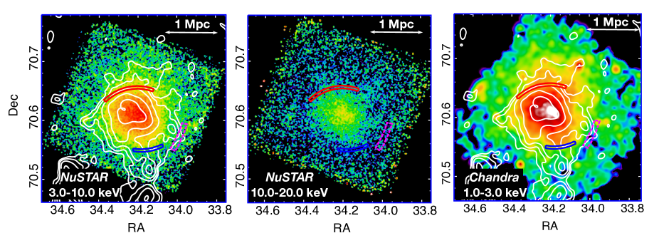
Figure 1: Background subtracted, exposure corrected photon images of CL 0217+70  in the 3.0 - 10.0 keV NuSTAR  (left panel), 10.0 - 20.0 keV NuSTAR  (middle panel), and 1.0 - 3.0 keV Chandra (right panel) bands. LOFAR contour levels (white) correspond to $\sigma_{rms}\times$ [3, 6, 12, 24, 48] ($\sigma_{rms}$ = 330 $\mu$Jy/beam [46$\arcsec\times$45$\arcsec$]) (Hoang et al., 2021). Red and blues arcs correspond to the location of northern and southern SB edges proposed by Zhang et al. (2020b), respectively. The channel region is indicated with dashed magenta rectangle.

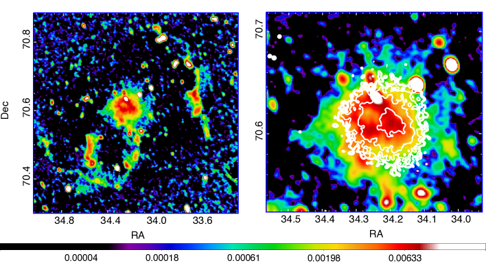
Figure 2: LOFAR 26.6$\arcsec$ $\times$ 22.5$\arcsec$ resolution image (Hoang et al., 2021) with 3.0-10.0 keV NuSTAR  contours overlaid.

In order to filter the data, standard pipeline processing using HEASoft (v. 6.28) and NuSTARDAS (v. 2.0.0.) tools are used. To clean the event files, the stage 1 and 2 of the NuSTARDAS pipeline processing script nupipeline are used. Regarding the cleaning of the event files for the passages through the South Atlantic Anomaly (SAA) and a “tentacle”-like region of higher activity near part of the SAA, instead of using SAAMODE=STRICT and TENTACLE=yes calls, we have created light curves and applied different filters to create good time intervals (GTIs) manually without fully discarding the passage intervals.

The new set of GTIs are reprocessed with nupipeline stages 1 and 2, and images are generated at different energy bands with XSELECT. To create exposure maps, nuexpomap are used. To produce the corresponding spectra for the regions of interest as well as the corresponding Response Matrix Files (RMFs) and Ancillary Response Files (ARFs), stage 3 of nuproducts pipeline are used.

Main components of the NuSTAR background are instrument Compton scattered continuum emission, instrument activation and emission lines, cosmic X-ray background from the sky leaking past the aperture stops, reflected solar X-rays, and focused and ghost-ray cosmic X-ray background. Modeling the background where there is a lack of cluster emission regions is not straightforward since the ICM emission becomes an additional component in the background fitting procedure. To apply these models for the cluster background assessment, a set of IDL routines called nuskybgd (Wik et al., 2014), which defines the background spatially and spectrally, is utilized.

The procedure starts with selecting regions in the FOV, where the cluster emission is inherently present yet not the most dominant. To account for the ICM emission, a single temperature apec model is included in the full set of models, and jointly fitted with the background components. The point sources detected in the Chandra FOV were not originally excluded from these regions, since they did not become apparent until after the background subtraction. While they may bias the focused cosmic X-ray background (fCXB) component in some regions, the average fCXB level is used to produce background spectra in all regions, lessening their impact, which is already only $\sim$10% of the total background. We discuss the systematics in Section A.

The global background model is then used to create background images, which are then subtracted from the images and are corrected by the corresponding exposure maps. Background subtracted, exposure corrected images at different energy bands are presented in the left and middle panels of Fig. 1. Region selection and the background fits are presented in Section A.

Once the background is defined for any region in the FOV both spatially and spectrally, the next step is to select regions of interest, to extract spectra and the corresponding files and generating the specific background model, followed by spectral fitting to evaluate the physical properties of the ICM.

2.2 Chandra

We use the observation and blank-sky background event files obtained from the 25 ks Chandra archival data (Observation ID: 16293) produced by Zhang et al. (2020b) for the data analysis. We use Chandra Interactive Analysis of Observations (CIAO) v4.12 package with CALDB 4.9.0 for extracting the spectra. Background subtracted, exposure corrected image in the 1.0 - 3.0 keV band are presented in the right panel of Fig. 1.

In addition to NuSTAR and Chandra data, we also represent the LOFAR data with courtesy of Hoang et al. (2021, Fig. 4). The LOFAR image of the cluster showing the relics and the central region is presented in Fig. 2.

3 Data analysis and results

3.1 Global properties

We began our analysis with the assessment of the global properties of the cluster. We selected a circular region centered at the X-ray emission peak with r = 5.2′  ($\sim$1 Mpc), following the extent of the radio halo emission. We extracted a spectrum from NuSTAR  which then was fit by a single temperature apec model (Smith et al., 2001), i.e. constant $\times$ apec, i.e. 1T model, with XSPEC (v. 12.11.1).

The redshift value of the cluster is freed to vary due to the gain issue of NuSTAR  (Rojas Bolivar et al., submitted). Once the best-fit values are found for the redshift, we then freeze these parameters during error calculations. We apply the maximum likelihood-based statistic (hereafter, C-stat) appropriate for Poisson data as proposed by Cash (1979). Photon counts used in spectral analysis are grouped to have at least 3 counts in each bin.

We then applied this method to the joint analysis of NuSTAR and Chandra data. For all of the joint analyses, we convolve the model with TBabs since Chandra is susceptible to N_H, and we let this parameter free. CL 0217+70 lies within 9° of the Galactic plane and consequently suffers from a high foreground column density ($N_{H}\sim 8\times 10^{21}$ cm^-2), which absorbs most X-ray photons with energies below a few keV. Near the plane, it is also expected that the column density will be variable on arcminute scales, which cannot be reliably predicted from HI estimates. Due to NuSTAR’s lack of bandpass sensitivity below 3 keV, we are able to the ignore foreground absorption at this level (Rojas Bolivar et al., 2021) for NuSTAR analysis for simplicity. However, we report $\sim$0.2 keV difference with/without the inclusion of an absorption model with $N_{H}\sim 8\times 10^{21}$ cm^-2 for the global fit. However, when the N_H parameter is freed to vary, the face value becomes 10¹⁷ cm^-2 where the lower limit hits the hard limit of zero with the higher limit reaching on to 10¹⁹ cm^-2. This unphysical behavior of the parameter points to NuSTAR’s lack of sensitivity to N_H at low energies.

Table 2: Spectral parameters and 1$\sigma$ uncertainty ranges of NuSTAR global spectrum fits in 3.0 - 20.0 band for 1T: constant $\times$ apec, 2T: constant $\times$ (apec + apec) and 1T + IC: constant $\times$ (apec + powerlaw). For the 2T model, abundance and redshift values of two apec components are tied to each other within instruments. apec normalization (n) is given in $\frac{10^{-14}}{4\pi\left[D_{A}(1+z)\right]^{2}}\int n_{e}n_{H}dV$ where powerlaw normalization ($\kappa$) is photons $\textit{keV}^{-1}~{}cm^{-2}~{}s^{-1}$ at 1 keV.

	1T	2T	1T + IC
kT1 (keV)	9.13 $\pm{0.12}$	10.60${}^{+0.79}_{-0.44}$	7.76${}^{+0.26}_{-0.25}$
Z1 (Z⊙)	0.198$\pm{0.026}$	0.280${}^{+0.034}_{-0.032}$	0.282${}^{+0.036}_{-0.034}$
z1	0.222	0.222	0.219
norm1 (10-2)	1.369 $\pm{0.018}$	1.139${}^{+0.060}_{-0.073}$	1.045${}^{+0.049}_{-0.046}$
kT2	$\cdots$	2.16${}^{+1.14}_{-0.52}$	$\cdots$
norm2 (10-2)	$\cdots$	0.728${}^{+0.312}_{-0.156}$	$\cdots$
$\Gamma$	$\cdots$	$\cdots$	2.0 (fixed)
$\kappa$ (10-2)	$\cdots$	$\cdots$	0.121${}^{+0.016}_{-0.018}$
C / $\nu$	1679.29/1686	1638.04/1684	1640.99/1685

Table 3: Same as Table 2 but for joint NuSTAR (3.0 - 20.0 keV) and Chandra (0.8 - 7.0 keV) joint global spectral fit. All models are convolved with TBabs. During the error calculations, redshifts (z) are fixed to the best-fit values. Subscripts “N” refer to NuSTAR, and “C” refer to Chandra parameters.

	1T	2T	1T + IC
NH (1021 cm-2)	9.17 $\pm{0.25}$	9.80$\pm{0.27}$	10.06$\pm{0.33}$
kT1 (keV)	9.20${}^{+0.11}_{-0.12}$	21.56${}^{+2.71}_{-2.90}$	7.99${}^{+0.25}_{-0.24}$
Z1N (Z⊙)	0.202 $\pm{0.026}$	0.214 $\pm{0.024}$	0.273${}^{+0.034}_{-0.033}$
Z1C (Z⊙)	0.550${}^{+0.110}_{-0.105}$	0.572${}^{+0.102}_{-0.097}$	0.750${}^{+0.135}_{-0.128}$
z1N	0.228	0.219	0.221
z1C	0.188	0.185	0.186
norm1 (10-2)	1.376$\pm{0.017}$	0.364${}^{+0.095}_{-0.062}$	1.081${}^{+0.048}_{-0.047}$
kT2	$\cdots$	6.36${}^{+0.40}_{-0.38}$	$\cdots$
norm2 (10-2)	$\cdots$	1.133${}^{+0.061}_{-0.096}$	$\cdots$
$\Gamma$	$\cdots$	$\cdots$	2.0 (fixed)
$\kappa$ (10-2)	$\cdots$	$\cdots$	0.107${}^{+0.018}_{-0.016}$
C / $\nu$	2104.29/2107	2067.33/2105	2071.99/2106

The spectral fit results of the parameters are presented in Table 2, and Table 3, for NuSTAR, and for joint NuSTAR and Chandra, respectively. To study the non-isothermal gas expected from merging clusters of galaxies, as well as possible non-thermal emission due to inverse Compton (IC) scattering, we applied two more models to the spectra following the work of Rojas Bolivar et al. (2021) and Wik et al. (2014).

We first added another apec component to the 1T model to describe a secondary temperature structure, and fitted the spectra with constant $\times$ (apec + apec), namely 2T model. We then used another model 1T+IC : constant $\times$ (apec + powerlaw), accounting for the thermal emission and a possible IC emission, where the IC component is represented with a power-law distribution. We fixed the photon index to $\Gamma$ = 2 of the powerlaw obtained from the spectral index found by Hoang et al. (2021).

The addition of a second apec and a powerlaw to the original single temperature model for NuSTAR  spectrum, resulted in an improvement of $\Delta$C/$\Delta\nu$ = 41.25/2 and $\Delta$C/$\Delta\nu$ = 38.30/1 for 2T and 1T + IC model, respectively, with respect to single temperature fit. For the joint NuSTAR and Chandra analysis, the fit also improved by an additional apec or a powerlaw component, where we found $\Delta$C/$\Delta\nu$ = 36.96/2 and $\Delta$C/$\Delta\nu$ = 32.30/1 for 2T and 1T + IC, respectively. Both NuSTAR, and joint NuSTAR and Chandra analysis show that the central r = 5.2′emission is best described by the 2T model.

We also calculated the luminosity of the cluster from the NuSTAR spectra within this region (r = 312$\arcsec$ $\simeq$ 0.6 R₅₀₀ adopting R₅₀₀ = 500$\arcsec$ (Reiprich et al., 2013)). We find the X-ray bolometric (0.01-100 keV) luminosity to be L_X,bol = 1.390 $\times$ 10⁴⁵ erg s^-1, and within 0.5-2.0 keV we find L_X,0.5-2.0keV = 2.716 $\times$ 10⁴³ erg s^-1 using ${\tt XSPEC}$ convolution model ${\tt clumin}$, for the 1T model.

NuSTAR gain issue is usually accommodated by the use of xspec gain command. The gain over the years shows an offset value around -0.1, but is still a work under construction (Rojas Bolivar et al., submitted). In the global spectral analysis using 1T model, we found that the gain is -0.15. When we use the gain command, the temperature becomes kT=9.15${}^{+0.17}_{-0.12}$ keV with 1684.29/1685 d.o.f., and the temperature is kT=9.13$\pm{0.12}$ keV with 1679.29/1686 d.o.f., when the redshift is freed to vary. Using the gain command instead of freeing the redshift changes the temperature by only 0.3%, but does not necessarily provide a better model. Due to the complexity of applying the gain command further in our analyses, we chose to free the redshift to account for the gain issue for the rest of this work.

In addition, here we share the luminosities that account for the evolution of the L_X-T scaling relations, using E(z)=1.09, where E(z)=$\sqrt{\Omega_{M}(1+z)^{3}+(1-{\Omega_{M}}-\Omega_{\Lambda})(1+z)^{2}+\Omega_{\Lambda}}$ (Giles et al., 2016). Diving the obtained luminosities by E(z), the luminosity values become L_X,bol = 1.275 $\times$ 10⁴⁵ erg s^-1 and L_X,0.5-2.0keV = 2.492 $\times$ 10⁴³ erg s^-1.

The resulting spectra are shown in Section B.

3.2 Surface brightness discontinuities

To study the correspondences of northern and southern Chandra SB edges (Fig. 1) with NuSTAR, we used Gaussian Gradient Magnitude (GGM) filter (Sanders et al., 2016). Assuming Gaussian derivatives with a width of $\sigma$, the GGM filter calculates the gradient of an image. To create the GGM filtered image, the image itself is convolved by the gradient of a 1D Gaussian function for two axes, then these two resulting images are combined for the 2D gradient image. The width, $\sigma$, is varied to capture gradients on different scales, i.e., small $\sigma$ values are used at the central regions where there are many counts, and high values are better capturing the gradient at cluster outskirts with low counts.

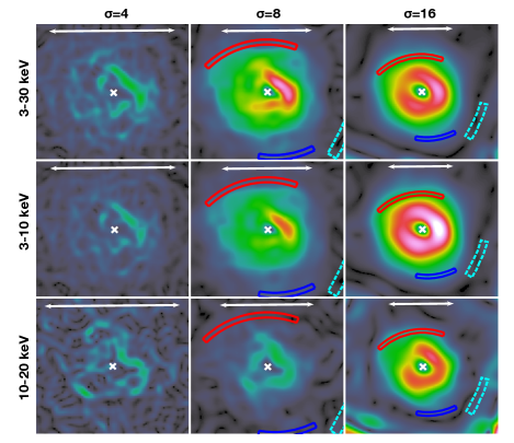
Figure 3: NuSTAR GGM filtered background subtracted, exposure corrected images in the 3.0 - 30.0 keV (top panels), 3.0 - 10.0 keV (middle horizontal panels), and 10.0 - 20.0 keV (lower panels) energy bands. White cross correspond to the emission peak, red (blue) arc corresponds to the northern (southern) SB edge, and dashed turquoise region represents the channel. The white arrow in all images correspond to 1 Mpc.

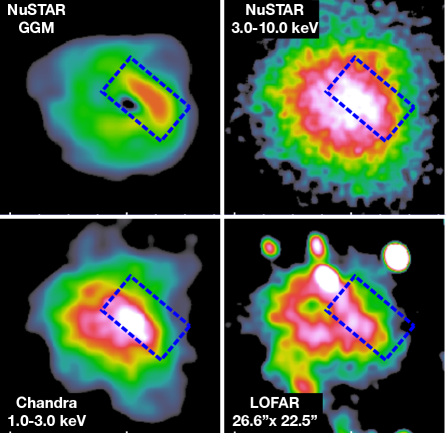
Figure 4: $\sigma$ = 8, 3.0 - 10.0 keV NuSTAR GGM (upper left ), NuSTAR  3.0 - 10.0 keV photon (upper right), Chandra 1.0 - 3.0 keV photon (lower left), and LOFAR 26.6$\arcsec$ $\times$ 22.5$\arcsec$ resolution (lower right) images. Dashed blue box corresponds to the same regions in all images .

Since NuSTAR PSF is much larger than the Chandra PSF for which the GGM filter was intended for, the filters with low levels of sigma ($\sigma$ = 1, 2) were mainly dominated by the noise. Therefore, we present the GGM filtered to the background subtracted, exposure corrected images with using $\sigma$ = 4, 8, and 16 detector pixels, as shown in Fig. 3.

Due to the large PSF of NuSTAR, the northern and southern SB edges are not unambiguously visible from the GGM results. We note that the SB edge and the channel locations obtained from Zhang et al. (2020b) are overlaid on the GGM (Fig. 3) merely to guide the eye and are not indicated by GGM analysis. The use of the GGM in this context is to reveal the strong SB feature much closer to the cluster center than the Chandra detected northern and southern SB edges.

GGM point to a sharp gradient best discerned in the panels presenting $\sigma$ = 8, 3.0 - 10.0 and 3.0 - 30.0 keV band, and $\sigma$ = 16, 3.0 - 10.0 keV band, suggesting a SB edge. This edge can also be seen in NuSTAR, Chandra, and LOFAR images. For a better visualization of this edge, we present the NuSTAR GGM, NuSTAR photon, Chandra photon, and LOFAR images together in Fig. 4.

3.3 Temperature map

To study the temperature structure of the NuSTAR FOV, we created a temperature map. We extracted count images from a 12$\arcmin$ $\times$ 12$\arcmin$ central box region of the cluster in the 3.0 - 5.0, 6.0 - 10.0, and 10.0 - 20.0 keV bands where the point sources detected by Chandra were excluded. We avoided the 5.0 - 6.0 keV band due to the existence of FeK complex. The background images and exposure maps were extracted for the same energy bands with nuskybgd and nuproducts, respectively.

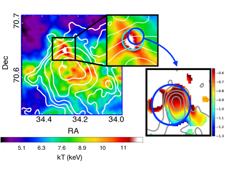
Figure 5: NuSTAR temperature map with radio contours from LOFAR (white, at $\sigma_{rms}\times$ [3, 6, 12, 24, 48], where $\sigma_{rms}$ = 330 $\mu$Jy/beam [46$\arcsec\times$45$\arcsec$]) are overlaid. In the zoomed in panel (black box, upper right corner), the “hot spot” is indicated by turquoise circle, and the radio source is shown with blue circle. In the lower right corner, the radio galaxy spectral map between 141 MHz (LOFAR) and 1.5 GHz (VLA) at 16$\arcsec$ resolution is shown (Hoang et al., 2021, Fig. 6).

The background subtracted, exposure corrected images were then used for the spectral extraction and predefined pixels were fitted with a single temperature apec model, during which the abundance and redshift were fixed to the values obtained from the global fit. The technique is described in detail by Markevitch et al. (2000). The resulting temperature map is presented in Fig. 5. We emphasize that this temperature map is a very basic analysis tool to search for any strong features in the ICM as in the case of the GGM analysis. We present more quantitative, accurate and precise temperature results further in the work.

In the temperature map, we encountered a “hot spot” that has a higher temperature than the cluster core. In the vicinity ($\sim$ 0.5$\arcmin$) of the “hot spot” (Fig. 5, turquoise circle), there is a radio source GB3 0212+704 (Maslowski, 1972) (Fig. 5, blue circle) and LOFAR high resolution study shows a tail morphology. The spectral index map between LOFAR 145 MHz and VLA 1.5 GHz also shows the steepening of the spectrum behind the tail. The tail radio galaxy has flux density of S (141 MHz) = 12.1$\pm$1.2 mJy, S (1.4 GHz)= 2.9 +/- 0.2 mJy, S (1.5 GHz)= 2.7 +/- 0.2 mJy. The average spectral index is $\alpha$= -0.62 $\pm$ 0.01.

Table 4: Spectral parameters and 1$\sigma$ uncertainty ranges of NuSTAR spectrum fits in 3.0 - 20.0 band of the “hot spot” scenarios.

	Hot spot	Obscured AGN	IC
NH (1022 cm-2)	$\cdots$	5.11 ${}^{+3.63}_{-3.52}$	$\cdots$
kT (keV)	12.10${}^{+2.01}_{-1.29}$	$\cdots$	$\cdots$
Z (Z⊙)	0.612 ${}^{+0.388}_{-0.312}$	$\cdots$	$\cdots$
z	0.249 ${}^{+0.046}_{-0.033}$	$\cdots$	$\cdots$
norm (10-4)	1.497 ${}^{+0.187}_{-0.158}$	$\cdots$	$\cdots$
$\Gamma$	$\cdots$	2.34 ${}^{+0.18}_{-0.17}$	2.13 ${}^{+0.09}_{-0.08}$
$\kappa$ (10-4)	$\cdots$	1.100${}^{+0.542}_{-0.356}$	0.657${}^{+0.120}_{-0.102}$
C / $\nu$	381.91/364	382.37/365	384.50/366

To study this feature in detail with NuSTAR, we extracted a circular region with r = 0.6$\arcmin$ ($\sim$112 kpc) enclosing the most dominant region of this “hot spot”, centered at 2:17:04.08 (RA) and +70:39:06 (Dec). The temperature map indicates that, if of thermal origin, the temperature of the plasma is $\geq$ 12 keV. This feature may be a part of a more extended emission, yet it is difficult define this extension.

To explain its nature, we put forward three scenarios. Scenario 1 suggests that the feature is the downstream shock region evidenced by its location on the northern Chandra SB edge. Scenario 2 is an emission from a heavily obscured AGN (since Chandra doesn not detect it) that may be due to a strong chaotic cold accretion (CCA) rain that feeds the central supermassive black hole (Gaspari et al., 2013, 2020). Scenario 3 is a localized IC emission where the electrons in the nearby radio source is upscattered to X-ray regime by a possible shock front.

We first fit the NuSTAR spectra with a single temperature apec model (Scenario 1). The temperature obtained from this fit was kT = 12.1${}^{+2.0}_{-1.3}$ keV with C/$\nu$ = 381.91/364. To test Scenario 2, we used a powerlaw model convolved with a TBabs model to account for a heavily obscured AGN. The resulting hydrogen column density value is N_H = 5.11$\times$10²² cm^-2, where the photon index for the hypothesized AGN emission is $\Gamma$ = 2.34${}^{+0.18}_{-0.17}$. The statistics of this fit is C/$\nu$ = 382.37/365. And for Scenario 3, we used an unabsorbed powerlaw model to describe possible IC emission. The resulting powerlaw slope is $\Gamma$ = 2.13${}^{+0.09}_{-0.08}$. The statistics of this fit is C/$\nu$ = 384.50/366. The corresponding values and spectra of the fits from these scenarios are presented in Table 4 and in Section C, respectively. Statistics show that these three scenarios are equally likely.

Lastly, to rule out a possible multi-temperature structure, we also fitted a two temperature model to the spectrum. The high temperature component rose up to kT $\sim$ 28.8 keV, where the low component was kT $\sim$ 7.41. In this fit, both temperature parameters were unconstrained.

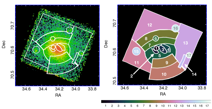
Figure 6: Regions selected for the cross-talk assessment.

3.4 Crosstalk analysis

Even single bright sources in the NuSTAR FOV causes the scatter photons due to the large ($\sim$1$\arcmin$ Half Power Diameter, $\sim$18$\arcsec$ Full Width at Half Maximum), slightly energy-dependent point spread function (PSF). This results in a cross-contamination, namely crosstalk, of multiple emission sources in the regions of interest, although the emission may not originate from the selected region. nuproducts produces ARFs for point or diffuse sources inside the user defined extraction regions. However, it does not account for the ARFs for other sources whose emission originates outside these extraction regions that contaminate the spectra of those regions. These ARFs will be referred to as cross-ARFs.

Software composed of a set of routines created to account for this contamination is nucrossarf.

In order to study the temperature jumps and prominent structures in the FOV more accurately, we selected regions of interest in the NuSTAR data and used nucrossarf to account for the crosstalk. The selected regions are overlaid on the NuSTAR image on the left panel, and the corresponding region values are presented in the right panel of Fig. 6.

Table 5: Crosstalk analysis spectral fit results where Region 6 is treated as a hot spot, obscured AGN and inverse Compton emission. In the obscured AGN scenario, the value N_H is kept fixed at 5.11 $\times$ 10²² cm^-2. ${\tt apec}$ normalization (norm) is given in $\frac{10^{-14}}{4\pi\left[D_{A}(1+z)\right]^{2}}\int n_{e}n_{H}dV$ (10^-3 cm^-5) where ${\tt powerlaw}$ normalization ($\kappa$) is photons keV^-1 cm^-2 s^-1 at 1 keV (10^-3).

	$kt$ (keV) or $\Gamma$				norm or $\kappa$
Region	nuproducts	nucrossarf			nuproducts	nucrossarf			Notes
Number		Hot spot	AGN	IC		Hot spot	AGN	IC
1	10.18${}^{+0.68}_{-0.33}$	9.90${}^{+1.90}_{-1.38}$	9.89${}^{+1.90}_{-1.38}$	9.90${}^{+1.90}_{-1.38}$	0.356${}^{+0.023}_{-0.021}$	0.459${}^{+0.056}_{-0.051}$	0.460${}^{+0.060}_{-0.051}$	0.459${}^{+0.056}_{-0.051}$
2	9.47${}^{+0.62}_{-0.73}$	7.47${}^{+2.44}_{-1.88}$	7.48${}^{+2.46}_{-1.87}$	7.43${}^{+2.45}_{-1.85}$	0.235${}^{+0.018}_{-0.019}$	0.217${}^{+0.061}_{-0.042}$	0.218${}^{+0.060}_{-0.042}$	0.219${}^{+0.061}_{-0.042}$
3	11.18${}^{+0.43}_{-0.20}$	12.53${}^{+0.94}_{-0.83}$	12.55${}^{+0.95}_{-0.82}$	12.51${}^{+0.94}_{-0.83}$	0.996${}^{+0.038}_{-0.034}$	1.406${}^{+0.060}_{-0.048}$	1.409${}^{+0.060}_{-0.048}$	1.407${}^{+0.061}_{-0.049}$	Cin
4	10.61${}^{+0.49}_{-0.46}$	10.29${}^{+0.93}_{-0.71}$	10.25${}^{+0.91}_{-0.71}$	10.31${}^{+0.92}_{-0.71}$	0.573${}^{+0.030}_{-0.028}$	0.800${}^{+0.041}_{-0.042}$	0.801$\pm{0.041}$	0.799${}^{+0.041}_{-0.042}$	Cout
5	9.92${}^{+0.16}_{-0.22}$	9.37${}^{+0.42}_{-0.44}$	9.35${}^{+0.42}_{-0.45}$	9.40${}^{+0.42}_{-0.44}$	3.452${}^{+0.089}_{-0.063}$	3.626${}^{+0.134}_{-0.123}$	3.635${}^{+0.139}_{-0.124}$	3.617${}^{+0.134}_{-0.121}$
6	12.02${}^{+1.76}_{-1.31}$	21.02	$\cdots$	$\cdots$	0.149${}^{+0.017}_{-0.016}$	0.108$\pm{0.012}$	$\cdots$	$\cdots$	Hot spot
6	2.34${}^{+0.18}_{-0.17}$	$\cdots$	2.34	$\cdots$	0.110${}^{+0.054}_{-0.036}$	$\cdots$	0.054$\pm{0.007}$	$\cdots$	AGN
6	2.13${}^{+0.09}_{-0.08}$	$\cdots$	$\cdots$	1.38$\pm{0.26}$	0.066${}^{+0.012}_{-0.010}$	$\cdots$	$\cdots$	0.014${}^{+0.010}_{-0.006}$	IC
7	9.29${}^{+0.27}_{-0.16}$	8.31${}^{+0.43}_{-0.41}$	8.57${}^{+0.45}_{-0.41}$	8.12${}^{+0.44}_{-0.40}$	1.862${}^{+0.051}_{-0.027}$	2.028${}^{+0.088}_{-0.082}$	2.014${}^{+0.084}_{-0.081}$	2.067${}^{+0.094}_{-0.089}$	Nin
8	7.51${}^{+0.30}_{-0.53}$	6.70${}^{+0.52}_{-0.47}$	6.98${}^{+0.54}_{-0.49}$	6.56${}^{+0.51}_{-0.47}$	1.449${}^{+0.055}_{-0.114}$	1.342${}^{+0.098}_{-0.090}$	1.319${}^{+0.093}_{-0.086}$	1.374${}^{+0.105}_{-0.095}$	Nout
9	8.98${}^{+0.39}_{-0.31}$	8.19${}^{+0.45}_{-0.44}$	8.20${}^{+0.45}_{-0.43}$	8.18${}^{+0.45}_{-0.43}$	1.527${}^{+0.061}_{-0.053}$	1.575${}^{+0.072}_{-0.064}$	1.578${}^{+0.072}_{-0.064}$	1.577${}^{+0.072}_{-0.065}$	Sin
10	8.05${}^{+0.72}_{-0.59}$	6.02${}^{+0.97}_{-0.72}$	6.02${}^{+0.97}_{-0.72}$	6.02${}^{+0.98}_{-0.72}$	0.819${}^{+0.055}_{-0.054}$	0.645${}^{+0.090}_{-0.082}$	0.646${}^{+0.090}_{-0.082}$	0.645${}^{+0.090}_{-0.082}$	Sout
11	7.13${}^{+0.54}_{-0.42}$	4.46${}^{+0.57}_{-0.62}$	4.44${}^{+0.56}_{-0.63}$	4.46${}^{+0.57}_{-0.61}$	1.195${}^{+0.075}_{-0.071}$	0.956${}^{+0.177}_{-0.112}$	0.960${}^{+0.181}_{-0.120}$	0.953${}^{+0.175}_{-0.119}$
12	4.72${}^{+0.29}_{-0.37}$	3.16${}^{+0.22}_{-0.20}$	3.15${}^{+0.22}_{-0.20}$	3.18${}^{+0.23}_{-0.21}$	2.921${}^{+0.226}_{-0.206}$	3.765${}^{+0.427}_{-0.380}$	3.803${}^{+0.426}_{-0.385}$	3.740${}^{+0.427}_{-0.379}$
13	9.97${}^{+0.82}_{-0.52}$	7.40${}^{+0.64}_{-0.60}$	7.37${}^{+0.63}_{-0.61}$	7.42${}^{+0.65}_{-0.60}$	1.819${}^{+0.104}_{-0.077}$	1.667${}^{+0.112}_{-0.107}$	1.672${}^{+0.123}_{-0.107}$	1.664${}^{+0.112}_{-0.107}$
14	8.25${}^{+2.26}_{-1.94}$	2.17${}^{+.....}_{-1.29}$	2.20${}^{+.....}_{-1.31}$	2.17${}^{+.....}_{-1.29}$	0.052${}^{+0.016}_{-0.013}$	0.140${}^{+......}_{-0.130}$	0.138${}^{+......}_{-0.128}$	0.141${}^{+......}_{-0.131}$	Channel
15	2.17$\pm{0.13}$	2.17	2.17	2.17	0.076${}^{+0.021}_{-0.017}$	0.040$\pm{0.006}$	0.040$\pm{0.006}$	0.040$\pm{0.006}$	PS
16	1.76${}^{+0.14}_{-0.13}$	1.76	1.76	1.76	0.041${}^{+0.012}_{-0.010}$	0.019$\pm{0.003}$	0.019$\pm{0.003}$	0.019$\pm{0.003}$	PS
17	2.79$\pm{0.17}$	2.79	2.79	2.79	0.183${}^{+0.062}_{-0.046}$	0.118${}^{+0.017}_{-0.016}$	0.118$\pm{0.016}$	0.118$\pm{0.016}$	PS

Table 6: Mach numbers of shock fronts calculated from the temperature jumps obtained from the crosstalk results..

Regions		Mach Number
Post-shock	Pre-shock	Hot spot	Obscured AGN	IC
3	4	1.22	1.22	1.21
6	8	2.01	$\cdots$	$\cdots$
7	8	1.24	1.23	1.24
9	10	1.37	1.37	1.37

The motivation behind selecting regions are based on the recent Chandra study proposing surface brightness edges, the results of our NuSTAR GGM and temperature map results, and LOFAR images. Region 1 corresponds to the radio SB depression as seen in the LOFAR image (Fig. 2, right panel). Region 2 is a wedge, again evidenced by LOFAR image. We selected these regions to investigate any correspondence of these radio features with the X-ray data. Regions 3 (C_in) and 4 (C_out) correspond to the inner and outer side of the central SB edge, respectively, as highlighted in Fig. 4. Region 5 represents the central region of the cluster that excludes the emission from Regions 1, 2, 3, and 4. Region 6 is the “hot spot”, which we investigate with the aforementioned three scenarios in Section 3.3.

Regions 7 (N_in) and 8 (N_out) are the inner (downstream) and outer (upstream) part of the northern SB edge proposed by Zhang et al. (2020b), respectively, and similarly, Regions 9 (S_in) and 10 (S_out) are the inner and outer sides of the southern SB, respectively. We note that Regions 7, 8, 9 and 10 are not the exact regions selected by Zhang et al. (2020b) that were used to draw the SB profiles on the corresponding edges in their work. The NuSTAR FOV ($13\arcmin\times 13\arcmin$) is considerably smaller than the Chandra FOV ($16\arcmin\times 16\arcmin$), and the regions they use for the SB profiles exceeds our FOV. We widened the angle of the southern and northern edge arcs to be able to capture as much upstream photons as possible for better statistics.

Regions 11, 12 and 13 indicate the outer cluster emission at different directions that is most likely isothermal. Channel is represented by Region 14. Finally, Regions 15, 16, and 17 are point sources as seen by Chandra and NuSTAR.

We extracted spectra from these 17 regions in total using nuproducts, and found the best fit model for these regions. In total, we have 13 regions to account for the ICM emission modeled by an apec, and 3 point sources (circular regions in Fig. 6) modeled by a powerlaw. And for Region 6, we use three different models as explained in detail in Section 3.3.

During the nucrossarf fit, we fitted 17 spectra, and their individual 17 ARFs simultaneously, where we fixed the redshift and abundance values to the individual nuproducts spectral fits. For Region 6, we studied the three scenarios. We ran the nucrossarf code thrice, first treating Region 6 as a hot spot, then obscured AGN and finally, localized IC emission. The results from the nuproducts and nucrossarf spectral analysis are given in Table 5.

We note that Region 14, where Chandra detects the possible SB depression (Channel), the upper limits for kT and apec normalization were quite large, therefore we constrained the upper limits to 9 keV and 1 $\times$ 10^-3 cm^-5 for the temperature and apec normalization, respectively.

For all of the AGN powerlaw models, we fixed the photon index to the nuproducts value to prevent an artificial gauge of any excess in the hard band regime by the powerlaw model. Since these regions are treated as point sources and since the regions attributed to them is comparable to the NuSTAR PSF, their emission should be localized, meaning the shape of the slope would be conserved.

To better visualise the effect of the inclusion of crosstalk analysis, we present temperature maps created by filling the regions of interest with the obtained temperature values from the fits in Fig. 7. This figure showing the temperature results from all scenarios are also a testament to the stability of the crosstalk analysis, as they visualize the almost identical temperature values when we assume difference emission models for Region 6.

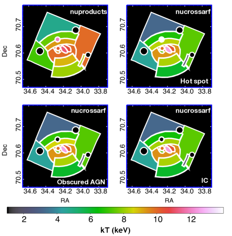
Figure 7: Temperature maps created with the results of nuproducts and nucrossarf analysis. We use color black to fill in the regions where a power-law model is used to describe the data, that is regions 15, 16 and 17 for all maps, and Region 6 for obscured AGN and IC scenarios.

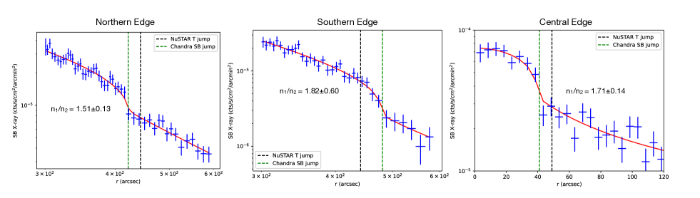
Figure 8: Chandra X-ray surface brightness profiles (blue) and the best-fit model (red) of northern, southern and central SB edges.

We then studied the Chandra SB profiles of the SB edges evidenced by NuSTAR, Chandra, LOFAR images, as well as our GGM analysis and temperature maps. These regions are 3 - 4 (C_in - C_out), 7 - 8 (N_in - N_out), and 9 - 10 (S_in - S_out), where the first region in these region couples are presumed post-shock and the second one represents the pre-shock.

Although Zhang et al. (2020b) study the SB profiles of northern and southern SB edges, we extracted new Chandra  SB profiles from the exact regions used in this work for precision. The profiles and the best fit model are shown in Fig. 8. Assuming the adiabatic index of an ideal monoatomic gas of $\gamma$=5/3, Mach numbers obtained from the density jumps are, $\mathcal{M}$ = 1.35, 1.58, and 1.50 for the northern, southern and central edges, respectively. The Mach numbers calculated by the temperature jumps from our crosstalk analysis range between 1.22 - 1.37. In addition, we calculated the Mach number for the temperature jump between regions 6-8, accounting for the possibility that “hot spot” is truly a hot plasma where the post-shock is localized at Region 6, i.e., a bullet-like feature, and Region 8 is the pre-shock region. This approach results in a $\mathcal{M}$ $\sim$ 2. These Mach numbers are presented in Table 6.

The details of the nucrossarf analysis are presented in Section D.

3.5 Local IC search

We did not find strong evidence for extended IC emission from our global spectra fit results, but we continued to search for IC locally within the radio halo, with the motivation that IC may start to dominate the emission in narrower regions moving away from the center of the cluster where ICM dominates. For this analysis, we used annular regions, where Hoang et al. (2021) studies radio spectral indices and we extracted NuSTAR spectra from 5 annuli as shown in Fig. 9. Although 6 regions are selected by Hoang et al. (2021, Fig. 7) including a central circular region, we exclude that central region from our analysis expecting for the ICM to dominate the total emission, hence we studied 5 annular regions. We applied the same analysis done for the NuSTAR global spectra to these annular spectra. We also allowed for metal abundances to be free. Model parameter results are shown in Table 7.

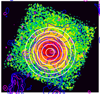
Figure 9: Selected regions (white annuli) for IC search overlaid on NuSTAR 3.0 - 10.0 keV image. VLA L-band D configuration (magenta, at 3$\sigma_{rms}\times$ [1, 2, 4, 8] levels, where ($\sigma_{rms}$ = 70 $\mu$Jy/beam), and LOFAR (blue, at $\sigma_{rms}\times$ [3, 6, 12, 24, 48]. ($\sigma_{rms}$ = 330 $\mu$Jy/beam [46$\arcsec\times$45$\arcsec$]) radio contours are also shown.

Annulus 1 spectrum is best described by a single temperature model, whereas for annuli 2 - 3 - 4, 2T model describes the spectra the best-fit models. The outermost annulus, annulus 5, is best described by 1T+IC model, but almost equally well as the 2T model does. This region roughly passes through the Regions 8 and 10 of our crosstalk analysis.

Table 7: IC search sprectral fit results from selected annuli shown in Fig. 9. Model norms are described in Table 2. IC flux is given for the 20.0 - 80.0 keV band in 10^-13 erg s^-1 cm^-2.

Annulus		$kt$	Z1	norm	$kt$ or $\Gamma$	norm or $\kappa$	IC
Number	Model	(keV)	(Z⊙)	(10-3)	keV or  $\cdots$	(10-3 cm-5) or (10-4)	Flux	C / $\nu$
1	1T	10.28${}^{+0.21}_{-0.20}$	0.31$\pm{0.06}$	2.808${}^{+0.062}_{-0.061}$	$\cdots$	$\cdots$	$\cdots$	1218.21 / 1318
	2T	10.34${}^{+0.23}_{-0.21}$	0.33${}^{+0.07}_{-0.06}$	2.786${}^{+0.065}_{-0.067}$	0.16${}^{+0.27}_{-0.13}$	5.390E7${}^{+1.572E10}_{-5.401E7}$	$\cdots$	1216.92 / 1316
	1T + IC	10.28${}^{+0.25}_{-0.28}$	0.31$\pm{0.07}$	2.373${}^{+0.102}_{-0.231}$	2.10 (fixed)	0.300${}^{+0.880}_{-0.300}$	0.46	1218.21 / 1317
2	1T	9.42${}^{+0.21}_{-0.20}$	0.31$\pm{0.06}$	2.846${}^{+0.069}_{-0.068}$	$\cdots$	$\cdots$	$\cdots$	1385.03 / 1365
	2T	10.34${}^{+0.91}_{-0.54}$	0.36$\pm{0.07}$	2.527${}^{+0.178}_{-0.371}$	2.33${}^{+2.13}_{-1.02}$	0.915${}^{+1.235}_{-0.423}$	$\cdots$	1380.11 / 1363
	1T + IC	8.90${}^{+0.37}_{-0.43}$	0.38${}^{+0.08}_{-0.07}$	2.384${}^{+0.239}_{-0.240}$	2.10 (fixed)	1.853${}^{+0.937}_{-0.934}$	2.85	1381.48 / 1364
3	1T	8.80${}^{+0.26}_{-0.27}$	0.13$\pm{0.06}$	2.165${}^{+0.066}_{-0.065}$	$\cdots$	$\cdots$	$\cdots$	1321.22 / 1351
	2T	12.91${}^{+2.71}_{-2.78}$	0.22${}^{+0.11}_{-0.08}$	1.371${}^{+0.329}_{-0.294}$	2.87${}^{+1.30}_{-1.64}$	1.689${}^{+1.809}_{-0.334}$	$\cdots$	1303.74 / 1349
	1T + IC	6.84${}^{+0.68}_{-0.60}$	0.24${}^{+0.09}_{-0.08}$	1.464${}^{+0.163}_{-0.162}$	2.05 (fixed)	2.842${}^{+0.611}_{-0.610}$	5.25	1306.49 / 1350
4	1T	7.34${}^{+0.28}_{-0.27}$	0.05${}^{+0.06}_{-0.05}$	1.897${}^{+0.079}_{-0.078}$	$\cdots$	$\cdots$	$\cdots$	1329.64 / 1361
	2T	7.70${}^{+0.39}_{-0.33}$	0.09${}^{+0.07}_{-0.06}$	1.778${}^{+0.094}_{-0.102}$	0.39${}^{+0.25}_{-0.16}$	1.271E4${}^{+2.378E8}_{-1.319E4}$	$\cdots$	1324.24 / 1359
	1T + IC	7.23${}^{+0.37}_{-0.59}$	0.05${}^{+0.06}_{-0.05}$	1.837${}^{+0.89}_{-0.215}$	2.10 (fixed)	0.231${}^{+0.841}_{-0.231}$	0.36	1329.53 / 1360
5	1T	7.38$\pm{0.39}$	0.12$\pm{0.08}$	1.491${}^{+0.087}_{-0.079}$	$\cdots$	$\cdots$	$\cdots$	1308.92 / 1435
	2T	24.40${}^{-25.08}_{-15.63}$	0.17${}^{+0.12}_{-0.08}$	0.348${}^{+0.722}_{-0.193}$	4.62${}^{+1.35}_{-2.57}$	1.457${}^{+0.208}_{-0.546}$	$\cdots$	1304.14 / 1433
	1T + IC	5.55${}^{+1.01}_{-1.14}$	0.26${}^{+0.19}_{-0.13}$	0.975${}^{+0.228}_{-0.198}$	2.15 (fixed)	2.300${}^{+0.798}_{-0.943}$	2.94	1304.25 / 1434

4 Summary and Discussion

CL 0217+70  hosts a giant radio halo and double radio relics pointing to a late stage merger. The location of radio relics points to a merger plane perpendicular to the line of sight. Motivated by the SB edges detected by Chandra (Zhang et al., 2020b) at the central region of the cluster, we observed the cluster with NuSTAR  with the aim of studying the nature of these SB edges. We applied spectro-imaging methods using NuSTAR and Chandra data, and relying on the recent LOFAR study by Hoang et al. (2021).

4.1 Global view

We first studied the photon images of NuSTAR, Chandra and LOFAR data. To capture any strong SB gradients, we used GGM filter on the NuSTAR  photon images and we saw that an interesting SB edge feature consistently appears at the central region of the cluster with NuSTAR, Chandra and LOFAR images as well as NuSTAR GGM filter.

Background extracted, exposure corrected images (Fig. 1) of NuSTAR and Chandra data point to a localized, enhanced emission at the central region, where we assigned Region 3 to, for our crosstalk analysis (Fig. 6). Furthermore, GGM and LOFAR images suggest a sharp edge between Regions 3 and 4, and the correspondence of this X-ray edge with the radio band, respectively, as seen in Fig. 4.

In addition, NuSTAR image at hard (10.0 - 20.0 keV) energy band hints at high temperature or the existence of non-thermal emission enclosed by the SB edges suggested by Zhang et al. (2020b) using Chandra  data. We found that the this hard excess is due to the hot ICM, given that we did not find strong IC component. We do not directly detect a clear SB depression at the proposed (Zhang et al., 2020b) “Channel” region from NuSTAR images.

The offset between the diffuse radio and X-ray central halo peak seen in the photon images (Fig. 1), as well as the NuSTAR SB and radio contours overlaid on the temperature map (Fig. 5), is also observed by Brown et al. (2011) for this cluster, as well as in Coma cluster Deiss et al. (1997). This is thought to be due the non-equilibrium state of the merger system (Brown et al., 2011).

The global analysis of the cluster constitutes the selection of a circular region (5.2$\arcmin$) containing the radio halo (roughly enclosing Regions 1-9), extraction of spectra of this region from both NuSTAR and Chandra data, and fitting the spectra with single temperature, two temperature and single temperature plus non-thermal emission models. The purpose of this analysis is to assess the global properties of the cluster and to search for possible extended IC emission in the cluster. Assuming an isothermal plasma, the global temperature found by NuSTAR is kT = 9.1$\pm{0.1}$ keV, and for joint NuSTAR and Chandra fit, we find kT = 9.2$\pm{0.3}$ keV. The results of NuSTAR, and joint NuSTAR and Chandra data analyses show that the statistics improve with an additional apec or powerlaw component, with respect to a single temperature apec model. The powerlaw component was more dominant in NuSTAR fit than joint NuSTAR and Chandra fit, due to the band pass of Chandra being narrower than that of NuSTAR. Therefore, joint fit captures more of the thermal emission. Two temperature model for the NuSTAR  fit has a high temperature component of T_H = 10.6${}^{+0.8}_{-0.4}$ keV and a lower temperature component with T_L = 2.2${}^{+1.1}_{-0.5}$ keV. However, our further detailed analyses on the temperature structure, i.e., temperature map and crosstalk analysis, do not show signs of dominant emission around this low temperature value. Apparently, the multi-temperature structure of the cluster would theoretically be better described with a multi-temperature model, yet the temperature values of various regions within the radio halo being high and close to each other makes it statistically difficult to disentangle these components.

In the joint NuSTAR and Chandra fit, however, we witnessed a subtle high temperature component of T_H = 21.56 ${}^{+2.71}_{-2.90}$ keV and a dominant low component of T_L = 6.4$\pm{0.4}$ keV. The lower limit found for Region 6 for the hot spot scenario in the crosstalk analysis results, is actually within 1$\sigma$ of this global high temperature component. The lower component, however, is too low with respect to what we see in the central region throughout this work, and also with respect to the findings of Zhang et al. (2020b, Table 1). Overall, the statistics for both NuSTAR, and joint NuSTAR and Chandra fit improved by adding a second apec model with $\Delta$C/$\Delta\nu$ = 41.25/2 and $\Delta$C/$\Delta\nu$ = 36.96/2, respectively.

The addition of a powerlaw component to the single temperature model improved the statistics by $\Delta$C/$\Delta\nu$ = 38.3/1 and $\Delta$C/$\Delta\nu$ = 32.3/1 for NuSTAR, and joint NuSTAR and Chandra analysis, respectively. Statistically a 2T fits the data better than a 1T+IC description (Table 2 and Table 3). The temperature component of the 1T+IC model is $\sim$8 keV. NuSTAR, and joint NuSTAR and Chandra analysis results agree within 1$\sigma$.

Although the data are better described by the 2T model, we provide an IC flux only to report an upper limit, as if IC were detected. The powerlaw component was more dominant in the NuSTAR fit than that of the joint fit. Therefore, we use NuSTAR fit results for our flux calculations. The upper limit to the IC flux in the 20.0 - 80.0 keV band was calculated using the cflux model applied to the powerlaw of the NuSTAR fit. The resulting flux is 2.695 $\times$ 10^-12 erg s^-1 cm^-2. Using the LOFAR data (Hoang et al., 2021), this refers to a lower limit of  0.08$\mu$G for the average magnetic field.

We also studied the effect of N_H parameter on our global spectra results using priors from Zhang et al. (2020b). Since our global region radius is $\sim$300″, the only prior we could use for N_H was fixing its value to 8.21$\times 10^{21}$ cm^-2 suggested by Zhang et al. (2020b), to test its impact on the global temperature and IC limit. By fixing the N_H to this value during the joint NuSTAR and Chandra 1T model fit, statistics become 2120.48/2108 d.o.f., where with free N_H, it is 2104.29/2107 d.o.f. Between these two approaches, the global temperature varies by 0.8%. And for the joint NuSTAR and Chandra 1T+IC model fit, fixing the N_H decreases the magnetic field lower limit by only 5% as opposed to letting it vary.

In addition, we studied the effect of the photon index, $\Gamma$, on the IC flux using our global joint NuSTAR and Chandra analysis (1T+IC model). We varied $\Gamma$ between 1.9 and 2.1 from the fixed value of $\Gamma$ = 2.0. $\Gamma$ = 2.0 is obtained from the spectral index ($\alpha$) value in Hoang et al. (2021). The uncertainty given by Hoang et al. (2021) on this $\alpha$ is +/-0.05, and here we use a more conservative approach by taking the error as +/-0.10. The IC flux changes by 9% and 12% for setting $\Gamma$ = 1.9 and $\Gamma$ = 2.1, respectively, instead of $\Gamma$ = 2.0.

4.2 The “hot spot”

Our temperature map in Fig. 5 shows a hot spot ($\sim$12 keV) at the location of the northern SB edge. We extracted NuSTAR spectra from this region to study the nature of the emission. We propose three scenarios to explain the emission from this source, which are (1) a hot spot where the shock heated gas is concentrated at that region (bullet-like), (2) a highly obscured AGN, and (3) a localized IC emission connected to the radio source in the vicinity.

Shocks driven by a piston-like object, like a cool core, do not produce shocks with uniform Mach number across it, but will have higher Mach numbers near the piston and lower farther away. If the “hot spot” is actually of thermal origin, this would be a similar case as in the bullet cluster. If the shock surface is considered as a 2D sheet, the middle will have the highest Mach number (in this case $\mathcal{M}$ = 2), and it will be lower everywhere else. At the hot spot-Region 8 interface the temperature jump will be highest and the particle acceleration will be most efficient.

Supported by theoretical and high-resolution hydrodynamical simulations (Gaspari et al. 2017, 2019), AGN in massive hot halos often become heavily obscured via the CCA triggered by the top-down multiphase condensation of warm and cold clouds, which rain onto the central supermassive black hole. Such obscuring CCA rain has been also probed in lower energy bands, e.g., with ALMA and MUSE absorption/emission-line features (Rose et al. 2019; Olivares et al. 2022; Temi et al. 2022).

However, at the “hot spot” location, there are no known AGNs. We also carried out a simple mid-IR selection criteria following (Somboonpanyakul et al., 2022) using AllWISE2020 Catalog . Within r=1$\arcmin$ of the “hot spot” position, we found an IR object with ID J021703.24+703909.0 and found W1-W2=-0.598. This value is much lower than what is expected from an AGN emission (Somboonpanyakul et al., 2022). However we note that, mid-IR selection for AGN mostly select extremely bright AGN (high accretion rate). This implies that the object may not be a strong AGN, but could still be a fainter/smaller AGN.

Furthermore, the vicinity of the radio galaxy may indeed be causing the IC emission due to the reacceleration of relativistic particles injected from the site, or by adiabatic compression, the merger shock may be “re-energizing” the radio plasma. The radio galaxy spectral index found by LOFAR is within 1$\sigma$ of the IC emission photon index we found.

Our NuSTAR analysis using nuproducts shows that all three scenarios are almost equally likely as represented in Table 4. However, 2T model fit to the joint NuSTAR and Chandra data revealing a similar high temperature (Table 3) for the global assessment with the crosstalk results for Region 6 of the hot spot (Table 5) may not be a coincidence. Although we would expect NuSTAR to capture the higher temperature component model better with respect to Chandra, the addition of the Chandra data may have helped better constraining the lower temperature model. Since Chandra data are quite shallow and foreground absorption is moderately high, it is difficult to make a conclusion.

4.3 Crosstalk analysis and Shock fronts

To account for the scattering due to NuSTAR PSF, we applied nucrossarf to dissociate the emission originating from a specific region, from the other regions in the field of view. Our crosstalk analysis (Table 5) reveal several temperature jumps between the regions selected with the guidance of NuSTAR, Chandra and LOFAR images, as well as temperature and GGM maps. These weak jumps occur at Region 7-8 (northern) and 9-10 (southern), and Region 3-4 (central) interface. We calculated Mach numbers for these jumps, and found $\mathcal{M}$ = 1.22 - 1.37 (Table 6), hinting at multiple weak shocks within the radio halo. Our Chandra SB profiles show that these temperature jumps have corresponding density jumps with $\mathcal{M}$ = 1.35 - 1.58. The Mach numbers derived from the NuSTAR temperature jumps and Chandra density jumps found in this work are consistent with each other. The Mach number obtained for the density jumps from the southern SB edge detected by Zhang et al. (2020b) is 2$\sigma$ higher than what we find in this work. We reason that the shock may be the strongest (localized) at the center when a smaller angle sector is selected for the analysis, as we similarly discuss in the case of the hot spot scenario in Section 4.2.

The physical distances of the temperature (density) jumps are $\sim$500 ($\sim$440) kpc, $\sim$650 ($\sim$780) kpc, and $\sim$100 ($\sim$72) kpc from the emission peak center for the northern, southern and central fronts, respectively. The difference between the locations of the temperature-density jumps may be due to the imperfect astrometry of NuSTAR, as well as the poor photon statistics of the Chandra data. Deeper Chandra observations could reveal more accurate and precise locations of the density jumps aided by Chandra GGM analysis followed by various deprojected radial SB profiles across the FOV.

On the technical side, we present a new code in this work, nucrossarf, aimed at accounting for the X-ray scattering in and out of spectral extraction regions within the NuSTAR FOV. We ran the code for three different scenarios for 17 sources, where the temperature and model normalization values of all sources are almost identical for the scenarios that points to the stability of the code. Furthermore, nucrossarf and nuproducts temperature values are in agreement within 1$\sigma$ for Regions 1-2-4-5-8-9 and 2$\sigma$ for Regions 3-7-10. Temperature values for Regions 11-12-13, that are at the outskirts of the cluster drop by $\sim$2 keV, pointing to a contamination of hard excess from the points sources enclosed by them, which is supported by the fact that the normalizations of these point source emissions are reduced by a factor of 2 after the crosstalk treatment. Regions 6- the “hot spot”, and Region 14 -the Channel temperatures from nuproducts are quite different from nucrossarf results.

For the “Channel” region, we see that the temperature and normalization parameters were poorly constrained. The scattered emission from the neighbouring regions may be responsible for this instability, hinting at a very faint emission at the Channel region.

The total fit C statistics for the crosstalk analyses are C/$\nu$ = 14669.14/15218, C/$\nu$= 14694.08/15219, C/$\nu$ = 14666.06/15218 for hot spot, obscured AGN, and IC scenarios that were assumed to explain the Region 6 emission, respectively. Although the best fit is obtained for the IC scenario, at this depth, all scenarios are almost equally likely.

4.4 IC search

We also carried out a local search for IC for regions where radio spectral indices are given by Hoang et al. (2021) inside the radio halo. The outermost annulus fit results show that 1T+IC model describes the spectra the best, but almost equally well with 2T model. For this region, we find an upper limit of 2.64 $\times$ 10^-13 erg s^-1 cm^-2 in the 20.0 - 80.0 keV band for the IC flux, if were detected. This region where 1T+IC model and 2T models have quite similar statistics, passes through Region 8 and 10 that is the outer region to the northern and southern shock fronts. Whereas annulus 3 has the highest IC flux, again has similar statistics with 2T model, and coincides with the northern and southern SB edges, that is expected due to shock enhancement (Sarazin, 2002, see, e.g.).

5 Conclusion

Based on the NuSTAR and Chandra data, complemented by a previous LOFAR study (Hoang et al., 2019), we studied the late stage galaxy cluster merger CL 0217+70 . We present our conclusions of this work in this section.

All three scenarios, namely; hot spot, obscured AGN and localized IC emission, proposed for the “hot spot” captured by our temperature map seem to be equally likely. If the “hot spot” is indeed a thermal plasma of $\sim$12 keV, it indicates a shock front $\sim$500 kpc away from the cluster emission peak. For the obscured AGN or IC emission scenarios deep optical and deep low frequency radio observations are required to study the galaxy distribution at the site. In essence, what is witnessed here may be even a combination of a hot spot + IC.

We confirm two shock fronts at Region 7-8 (northern) and 9-10 (southern) suggested by Zhang et al. (2020b), and detect another shock front at Region 3-4 interface (central), within 0.5 r₅₀₀ of the cluster. The physical distances of the temperature (density) jumps are $\sim$500 ($\sim$440) kpc, $\sim$650 ($\sim$780) kpc, and $\sim$100 ($\sim$72) kpc from the emission peak center for the northern, southern and central fronts, respectively. These weak shocks may be partially responsible for sustaining the giant radio halo emission by the (re)acceleration of the relativistic particles at the central region of the cluster.

The axis connecting these northern and southern secondary shock fronts are almost perpendicular to the axis connecting the radio relics, suggesting that these secondary shocks are unrelated to the first core passage. The coincidence of the northern and southern shock fronts with the radio halo emission edge adds this cluster a short list of clusters that suggests the radio halos formation may be boosted by the turbulence formed directly behind shocks. Deeper high angular resolution X-ray observations should reveal $\sim$ 100 kpc scale turbulence eddies, taking advantage of the merger plane lying perpendicular to the line of sight.

To the best of our knowledge, this cluster is the second known case where a secondary shock coinciding with the radio halo emission in the form of subsequent settling of the ICM is observed within 1 Mpc, the first being Coma (Simionescu et al., 2013).

Unlike Coma, CL 0217+70 shows multiple shock fronts, which makes this cluster the only known case where multiple secondary shock fronts are formed within 0.5 r₅₀₀. We may have captured this cluster before the settling of the ICM, hence, further studies beyond local systems are needed to be the carried out to investigate the ubiquity of these secondary shocks to understand the evolution of galaxy cluster mergers and radio halo formation mechanisms. Galaxy clusters hosting giant radio halos can be the first place to look for similar cases.

Appendix A NuSTAR Background assessment and systematics

In this section, we present the spectra from the background model fits using both FPMs and both Obs. ID in Fig. 10. As shown in the left panel of Fig. 10, we selected 4 regions in the FOV from each detector chip, excluding the ICM emission as much as possible but also including as much data as available. Region selection is somewhat an experienced guess, and we tested the fits for smaller and larger regions to optimize the stability of the fit. The method is described in Wik et al. (2014).

In addition, we note that single temperature apec model is sufficient to account for local and scattered cluster emission inside background regions, and more complicated models (e.g., two temperature apec model) do provide significant improvement. More importantly, the additional component, if not limited by strict priors, will generally try to model some other feature of the ICM spectra where the background model is not perfect.

To quantify the systematics of the fCXB in the NuSTAR  background analysis (Wik et al., 2014), we chose Region 5 that has the least complicated thermal structure. We increased and decreased the fCXB component of the background by 50% in the spectral fits to see its effect on the temperature measurements. We chose 50% since, given the cosmic variance for a region of this size, it is the expected variation in CXB that is also comparable to the brightness of the detected point sources. Increasing the fCXB component of the background by 50% resulted in a temperature decrease of 0.04 keV, whereas decreasing the fCXB component of the background by 50% resulted in a 0.06 keV increase in the temperature. These values correspond to less than 35% of the statistical errors on the temperature of that region.

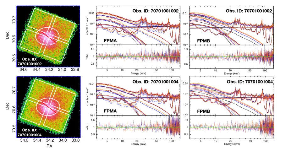
Figure 10: Selected regions for background analysis (left panel) laid over cleaned NuSTAR 3-10 keV photon images. White squares indicate regions where the background spectra is extracted. Joint-fit of background and cluster emission of NuSTAR FPMA (middle panel) and FPMB (right panel) for Obs. ID 70701001002 (upper panel) and Obs. ID 70701001004 (lower panel). Each color represents a region selected for the background fit. For plotting purposes, adjacent bins are grouped until they have a significant detection at least as large as 15$\sigma$, with maximum 15 bins.

The dominant systematic uncertainty of the NuSTAR background comes from the aperture cosmic X-ray background (aCXB) characterization, which dominates the $E\sim$10 keV background, but it is generally too flat to bias the thermal continuum and thus temperature measurements (Wik et al., 2014). This statement is less true when an IC model is included, but since the data do not support IC emission over pure thermal emission, the effect of this systematic uncertainty is negligible concerning our results.

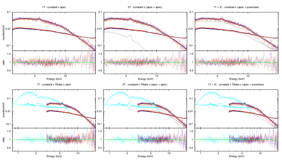
Figure 11: Global fits of NuSTAR (upper panel), and joint NuSTAR and Chandra data (lower panel) with 1T (left panel), 2T (middle panel), and 1T + IC (right panel) of the spectra extracted from the central 5$\arcmin$.2 circular region. Black indicates FPMA and red indicates FPMB for ObsID 70701001002, whereas for ObsID 70701001004, FPMA and FPMB are indicated by blue and orange, respectively. Chandra ACIS-I is indicated by turquoise. The data and models are shown as the higher curve and lower lines correspond to background spectrum. The dashed curves correspond to the model components to visualize their contribution to the composed model. The “ratio” panel shows data to model ratios describing the goodness of the fit. For plotting purposes, adjacent bins are grouped until they have a significant detection at least as large as 8$\sigma$, with maximum 12 bins.

Appendix B NuSTAR and Chandra global fit spectra

We present the results of the global spectral fit in this section for only NuSTAR and joint NuSTAR and Chandra data using 1T, 2T, and 1T + IC models as shown in Fig. 11. Since the statistics are quite similar, the differences in ratios are not discernible, yet the model contribution curves provide an insight to the contribution of different models.

Appendix C “hot spot” scenarios

The resulting spectra from the three scenarios proposed for the explanation of the Region 6 emission is presented in this section. The statistics are again similar, which makes it difficult to conclude from the figures which model best describes the data. However, in its spectrum we encountered a strange dip around 4.8 keV in Fig. 12. We extracted a spectra from a larger (1$\arcmin$) circular region at the location at the “hot spot”, as well as different data and plotting bins. The dip feature still persists for those spectra as well, pointing to a reason different from a mere coincidence of statistical fluctuations. We could not found an explanation for this feature, and we refrain from any speculations.

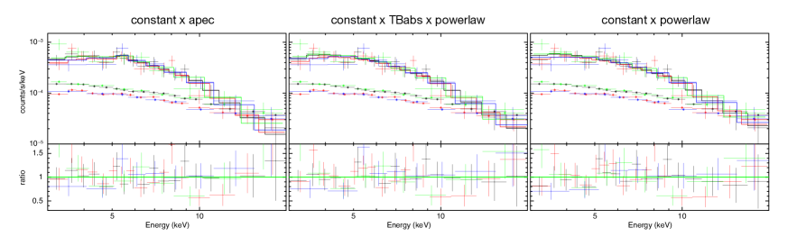
Figure 12: Spectra of the NuSTAR “hot spot” region fits with constant $\times$ apec (left panel), constant $\times$ TBabs $\times$ powerlaw (middle panel), and constant $\times$ powerlaw (right panel). Black indicates FPMA and red indicates FPMB for ObsID 70701001002, whereas for ObsID 70701001004, FPMA and FPMB are indicated by green and blue, respectively. For plotting purposes, adjacent bins are grouped until they have a significant detection at least as large as 4$\sigma$, with maximum 8 bins.

Appendix D nucrossarf

With this detailed study, we also happen to test the new nucrossarf code. In this section, we elaborate the inner workings of the code, and what to expect from the code for future users.

nucrossarf mainly calculates the cross-ARFs of a number of user defined extracted regions, and dissociates the source distribution from the contamination from other regions by jointly fitting the spectra of all regions. For N extracted regions, nucrossarf generates N $\times$ N ARFs to account for the wings of the PSF of each source present in other regions.

The final fitted spectra for the obscured AGN scenario is presented in the left panel of Fig. 13 as an example. This figure shows the spectra from each source, the total ARF curve and the individual contributions from all regions, for two observations and for both FPMA and FPMB: (1+1+17) $\times$ 2 $\times$ 2 curves in total. In order to present a much less complicated version, we plotted the spectrum from Region 1, the total ARF curve and the individual contributions from all regions to Region 1 emission, for Obs ID 70701001002 and for FPMA as seen in the right panel of Fig. 13

As seen in the nucrossarf spectral fit of Region 1 spectra for ObsID 70701001002 FPMA, the shape of the weakest model seen in the right panel in Fig. 13 has an artifact- a dip within 5.0 - 10.0 keV. This model corresponds to the scattering from Region 17 to Region 1. We further investigated the spectra for similar artifacts and saw that point source crosstalk contributions to the regions that are far away from these sources show a similar behaviour. These curves are 15-10, 15-4, 16-2, 16-9, 16-14, 16-17, 17-1, 17-2, 17-12, 17-16, where the first numbers in the couples point to the origin of the scattered light, and the seconds correspond to where the scattered light reaches. These crossarfs with artifacts for Obs ID 70701001002 are plotted in the lower panel of Fig. 14, where the upper panel shows the entirety of the ARFs.

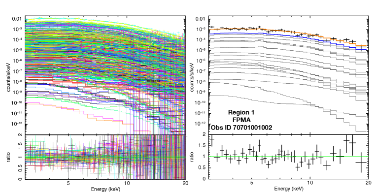
Figure 13: Total cross-talk spectra for the AGN scenario final fit, (left panel) and the spectra for the AGN scenario, for Region 1, ObsID 70701001002 FPMA (right panel). In the right panel, black indicates the data, orange presents the total model, blue curve is the local contribution model from Region 1 and gray curves represent the scattering from other regions.

Since for the production of ARFs, the PSF images at various bands are used, these artifacts are bound to happen for faint point sources that are close to the edge of the FOV where the calibration for PSF is less than perfect. nucrossarf samples the PSF images for extended sources therefore averaging out very small fluctuations. Therefore we do not see any similar artifacts from Region 14, Channel, which is also close to the edge of the FOV and has faint emission. At very low effective area, the level of the artifacts are comparable to data noise. We emphasize that, at this rate, ARF contributions where we see the dip artifact are effectively zero ($\sim$10^-9 counts/s) and the artifacts do not have an effect on any of our results.

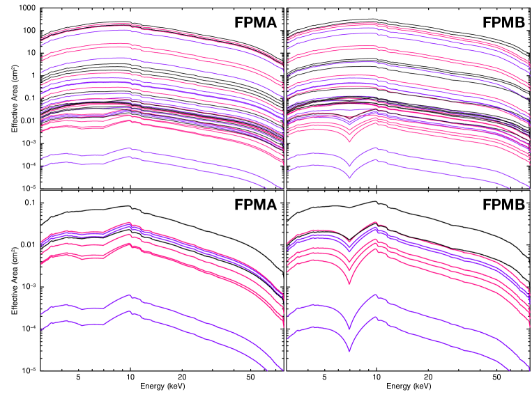
Figure 14: All cross-ARFs for Region 15 (black), 16 (purple) and 17 (pink) from Obs ID 70701001002 (upper panel), and only the cross-ARFs of artifacts (lower panel), namely cross-ARFs: 15-10, 15-4, 16-2, 16-9, 16-14, 16-17, 17-1, 17-2, 17-12, and 17-16.

References

- Abell (1958) Abell, G. O. 1958, ApJS, 3, 211, doi: 10.1086/190036
- Brown et al. (2011) Brown, S., Duesterhoeft, J., & Rudnick, L. 2011, ApJ, 727, L25, doi: 10.1088/2041-8205/727/1/L25
- Brown & Rudnick (2011) Brown, S., & Rudnick, L. 2011, Monthly Notices of the Royal Astronomical Society, 412, 2, doi: 10.1111/j.1365-2966.2010.17738.x
- Brunetti et al. (2012) Brunetti, G., Blasi, P., Reimer, O., et al. 2012, Monthly Notices of the Royal Astronomical Society, 426, 956, doi: 10.1111/j.1365-2966.2012.21785.x
- Brunetti & Jones (2014) Brunetti, G., & Jones, T. W. 2014, International Journal of Modern Physics D, 23, 1430007, doi: 10.1142/S0218271814300079
- Cash (1979) Cash, W. 1979, ApJ, 228, 939, doi: 10.1086/156922
- Cassano et al. (2010) Cassano, R., Ettori, S., Giacintucci, S., et al. 2010, ApJ, 721, L82, doi: 10.1088/2041-8205/721/2/L82
- Clavico et al. (2019) Clavico, S., De Grandi, S., Ghizzardi, S., et al. 2019, A&A, 632, A27, doi: 10.1051/0004-6361/201936467
- Cova et al. (2019) Cova, F., Gastaldello, F., Wik, D. R., et al. 2019, A&A, 628, A83, doi: 10.1051/0004-6361/201834644
- De Grandi et al. (2016) De Grandi, S., Eckert, D., Molendi, S., et al. 2016, A&A, 592, A154, doi: 10.1051/0004-6361/201526641
- Deiss et al. (1997) Deiss, B. M., Reich, W., Lesch, H., & Wielebinski, R. 1997, A&A, 321, 55. https://arxiv.org/abs/astro-ph/9609189
- Eckert et al. (2017) Eckert, D., Gaspari, M., Vazza, F., et al. 2017, ApJ, 843, L29, doi: 10.3847/2041-8213/aa7c1a
- Ensslin et al. (1998) Ensslin, T. A., Biermann, P. L., Klein, U., & Kohle, S. 1998, A&A, 332, 395. https://arxiv.org/abs/astro-ph/9712293
- Feretti et al. (2012) Feretti, L., Giovannini, G., Govoni, F., & Murgia, M. 2012, A&A Rev., 20, 54, doi: 10.1007/s00159-012-0054-z
- Gabici & Blasi (2003) Gabici, S., & Blasi, P. 2003, ApJ, 583, 695, doi: 10.1086/345429
- Gaspari (2015) Gaspari, M. 2015, MNRAS, 451, L60, doi: 10.1093/mnrasl/slv067
- Gaspari & Churazov (2013) Gaspari, M., & Churazov, E. 2013, A&A, 559, A78, doi: 10.1051/0004-6361/201322295
- Gaspari et al. (2013) Gaspari, M., Ruszkowski, M., & Oh, S. P. 2013, Monthly Notices of the Royal Astronomical Society, 432, 3401, doi: 10.1093/mnras/stt692
- Gaspari et al. (2017) Gaspari, M., Temi, P., & Brighenti, F. 2017, MNRAS, 466, 677, doi: 10.1093/mnras/stw3108
- Gaspari et al. (2020) Gaspari, M., Tombesi, F., & Cappi, M. 2020, Nature Astronomy, 4, 10, doi: 10.1038/s41550-019-0970-1
- Gaspari et al. (2019) Gaspari, M., Eckert, D., Ettori, S., et al. 2019, ApJ, 884, 169, doi: 10.3847/1538-4357/ab3c5d
- Giles et al. (2016) Giles, P. A., Maughan, B. J., Pacaud, F., et al. 2016, A&A, 592, A3, doi: 10.1051/0004-6361/201526886
- Giovannini & Feretti (2004) Giovannini, G., & Feretti, L. 2004, Journal of Korean Astronomical Society, 37, 323, doi: 10.5303/JKAS.2004.37.5.323
- Harrison et al. (2013) Harrison, F. A., Craig, W. W., Christensen, F. E., et al. 2013, ApJ, 770, 103, doi: 10.1088/0004-637X/770/2/103
- Hlavacek-Larrondo et al. (2017) Hlavacek-Larrondo, J., Gendron-Marsolais, M.-L., Fecteau-Beaucage, D., et al. 2017, Monthly Notices of the Royal Astronomical Society, 475, 2743, doi: 10.1093/mnras/stx3160
- Hoang et al. (2019) Hoang, D. N., Shimwell, T. W., van Weeren, R. J., et al. 2019, A&A, 622, A20, doi: 10.1051/0004-6361/201833900
- Hoang et al. (2021) Hoang, D. N., Zhang, X., Stuardi, C., et al. 2021, A&A, 656, A154, doi: 10.1051/0004-6361/202141428
- Hofmann et al. (2016) Hofmann, F., Sanders, J. S., Nandra, K., Clerc, N., & Gaspari, M. 2016, A&A, 585, A130, doi: 10.1051/0004-6361/201526925
- Markevitch et al. (1999) Markevitch, M., Sarazin, C. L., & Vikhlinin, A. 1999, ApJ, 521, 526, doi: 10.1086/307598
- Markevitch et al. (2000) Markevitch, M., Ponman, T. J., Nulsen, P. E. J., et al. 2000, ApJ, 541, 542, doi: 10.1086/309470
- Maslowski (1972) Maslowski, J. 1972, Acta Astron., 22, 227
- Olivares et al. (2022) Olivares, V., Salome, P., Hamer, S. L., et al. 2022, arXiv e-prints, arXiv:2201.07838. https://arxiv.org/abs/2201.07838
- Planck Collaboration et al. (2013) Planck Collaboration, Ade, P. A. R., Aghanim, N., et al. 2013, A&A, 554, A140, doi: 10.1051/0004-6361/201220247
- Reiprich et al. (2013) Reiprich, T. H., Basu, K., Ettori, S., et al. 2013, Space Sci. Rev., 177, 195, doi: 10.1007/s11214-013-9983-8
- Rojas Bolivar et al. (2021) Rojas Bolivar, R. A., Wik, D. R., Giacintucci, S., et al. 2021, ApJ, 906, 87, doi: 10.3847/1538-4357/abcbf7
- Rose et al. (2019) Rose, T., Edge, A. C., Combes, F., et al. 2019, MNRAS, 489, 349, doi: 10.1093/mnras/stz2138
- Ryu et al. (2003) Ryu, D., Kang, H., Hallman, E., & Jones, T. W. 2003, The Astrophysical Journal, 593, 599–610, doi: 10.1086/376723
- Sanders et al. (2016) Sanders, J. S., Fabian, A. C., Russell, H. R., Walker, S. A., & Blundell, K. M. 2016, MNRAS, 460, 1898, doi: 10.1093/mnras/stw1119
- Sarazin (2002) Sarazin, C. L. 2002, in Astrophysics and Space Science Library, Vol. 272, Merging Processes in Galaxy Clusters, ed. L. Feretti, I. M. Gioia, & G. Giovannini, 1–38, doi: 10.1007/0-306-48096-4_1
- Schellenberger et al. (2019) Schellenberger, G., David, L., O’Sullivan, E., Vrtilek, J. M., & Haines, C. P. 2019, The Astrophysical Journal, 882, 59, doi: 10.3847/1538-4357/ab35e4
- Shimwell et al. (2014) Shimwell, T. W., Brown, S., Feain, I. J., et al. 2014, Monthly Notices of the Royal Astronomical Society, 440, 2901, doi: 10.1093/mnras/stu467
- Simionescu et al. (2013) Simionescu, A., Werner, N., Urban, O., et al. 2013, ApJ, 775, 4, doi: 10.1088/0004-637X/775/1/4
- Smith et al. (2001) Smith, R. K., Brickhouse, N. S., Liedahl, D. A., & Raymond, J. C. 2001, ApJ, 556, L91, doi: 10.1086/322992
- Somboonpanyakul et al. (2022) Somboonpanyakul, T., McDonald, M., Noble, A., et al. 2022, AJ, 163, 146, doi: 10.3847/1538-3881/ac5030
- Temi et al. (2022) Temi, P., Gaspari, M., Brighenti, F., et al. 2022, ApJ, 928, 150, doi: 10.3847/1538-4357/ac5036
- Tümer et al. (2019) Tümer, A., Tombesi, F., Bourdin, H., et al. 2019, A&A, 629, A82, doi: 10.1051/0004-6361/201935660
- Tümer et al. (2022) Tümer, A., Wik, D. R., Gaspari, M., et al. 2022, ApJ, 930, 83, doi: 10.3847/1538-4357/ac61de
- van Weeren et al. (2019) van Weeren, R. J., de Gasperin, F., Akamatsu, H., et al. 2019, Space Sci. Rev., 215, 16, doi: 10.1007/s11214-019-0584-z
- van Weeren et al. (2016) van Weeren, R. J., Brunetti, G., Brüggen, M., et al. 2016, ApJ, 818, 204, doi: 10.3847/0004-637X/818/2/204
- Vikhlinin et al. (2009) Vikhlinin, A., Burenin, R. A., Ebeling, H., et al. 2009, ApJ, 692, 1033, doi: 10.1088/0004-637X/692/2/1033
- Wik et al. (2011) Wik, D. R., Sarazin, C. L., Finoguenov, A., et al. 2011, ApJ, 727, 119, doi: 10.1088/0004-637X/727/2/119
- Wik et al. (2014) Wik, D. R., Hornstrup, A., Molendi, S., et al. 2014, ApJ, 792, 48, doi: 10.1088/0004-637X/792/1/48
- Wittor & Gaspari (2020) Wittor, D., & Gaspari, M. 2020, MNRAS, 498, 4983, doi: 10.1093/mnras/staa2747
- Yang et al. (2019) Yang, H. Y. K., Gaspari, M., & Marlow, C. 2019, ApJ, 871, 6, doi: 10.3847/1538-4357/aaf4bd
- Zhang et al. (2020a) Zhang, C., Churazov, E., Dolag, K., Forman, W. R., & Zhuravleva, I. 2020a, MNRAS, 498, L130, doi: 10.1093/mnrasl/slaa147
- Zhang et al. (2020b) Zhang, X., Simionescu, A., Kaastra, J. S., et al. 2020b, A&A, 642, L3, doi: 10.1051/0004-6361/202039028