Black bounces, wormholes, and partly phantom scalar fields

Abstract

Simpson and Visser recently proposed a phenomenological way to avoid some kinds of space-time singularities by replacing a parameter whose zero value corresponds to a singularity (say, $r$) with the manifestly nonzero expression $r(u)=\sqrt{u^{2}+b^{2}}$, where $u$ is a new coordinate, and $b={\rm const}>0$. This trick, generically leading to a regular minimum of $r$ beyond a black hole horizon (called a “black bounce”), may hopefully mimic some expected results of quantum gravity, and was previously applied to regularize the Schwarzschild, Reissner-Nordström, Kerr and some other metrics. In this paper it is applied to regularize the Fisher solution with a massless canonical scalar field in general relativity (resulting in a traversable wormhole) and a family of static, spherically symmetric dilatonic black holes (resulting in regular black holes and wormholes). These new regular metrics represent exact solutions of general relativity with a sum of stress-energy tensors of a scalar field with nonzero self-interaction potential and a magnetic field in the framework of nonlinear electrodynamics with a Lagrangian function ${\mathcal{L}}({\mathcal{F}})$, ${\mathcal{F}}=F_{\mu\nu}F^{\mu\nu}$. A novel feature in the present study is that the scalar fields involved have “trapped ghost” properties, that is, are phantom in a strong-field region and canonical outside it, with a smooth transition between the regions. It is also shown that any static, spherically symmetric metric can be obtained as an exact solution to the Einstein equations with the stress-energy tensor of the above field combination.

I Introduction

There seems to be a common belief that quantum gravity effects inevitably suppress space-time singularities existing in the solutions of classical gravity, replacing them with some regular phenomena. Though, different approaches and models of quantum gravity, when translated to the classical language, lead to radically different results, see, e.g., [1, 2, 3, 4, 5, 6, 7, 8], and a discussion in [9]. Among them are black hole-white hole transitions [2, 3, 4, 5], scenarios with the spherical radius tending to a nonzero constant at late times beyond an event horizon [6], quantum-corrected configurations without horizons [8], etc. This diversity may be treated as a consequence of a still uncertain nature of quantum gravity by now.

Therefore, of evident interest is the recent proposal made by Simpson and Visser (SV) [10] to regularize a singular space-time metric by simply replacing its certain parameter (specifically, the spherical radius $r$ in a static, spherically symmetric metric), whose zero value corresponds to a singularity, with the simple expression $r(u)=\sqrt{u^{2}+b^{2}}$, where $u\in{\mathbb{R}}$ is a new coordinate introduced instead of $r$, and $b>0$ is a regularization parameter. It looks as an easy way to imagine the possible effects of quantum gravity within a classical space-time framework, leaving aside any quantization details. Besides, new geometries emerging in this way may be of interest by themselves.

In [10] this proposal was applied to the Schwarzschild black hole solution, resulting in the globally regular metric

$$ds^{2}=\bigg{(}1-\frac{2m}{\sqrt{u^{2}+b^{2}}}\bigg{)}dt^{2}-\bigg{(}1-\frac{2m}{\sqrt{u^{2}+b^{2}}}\bigg{)}^{-1}du^{2}-(u^{2}+b^{2})(d\theta^{2}+\sin^{2}\theta d\varphi^{2}),$$ (1)

where the singularity at $r=0$ is replaced by a regular minimum of $r(u)$ at $u=0$, a sphere of radius $b$. Depending on the relation between $b$ and the Schwarzschild mass $m$, the geometry (1) can represent a wormhole  with a throat at $u=0$ (if $b>2m$, hence $g_{tt}(0)>0$), a black hole with two horizons at $u=\pm\sqrt{4m^{2}-b^{2}}$ if $b<2m$, and an extremal black hole with a single horizon at $u=0$ if $b=2m$.

In the black hole case $b<2m$, the hypersurface $u=0$, being a minimum of $r(u)$, is not a throat since $u$ is a temporal coordinate there: instead, $u=0$ corresponds to a bounce in one of the two scale factors, $r(u)$, of a Kantowski-Sachs cosmology in the inner region of the black hole, and by SV suggestion such a minimum is called a black bounce [10]. (The other scale factor in this Kantowski-Sachs cosmology is $2m/\sqrt{u^{2}+b^{2}}-1$, and it has a maximum at the same time instant $u=0$.) It can be noted that black bounces are a common feature of another class of space-times, black universes, that is, black holes that contain an expanding asymptotically isotropic cosmology beyond the horizon [11, 12, 13]. Such solutions are naturally obtained with a phantom scalar field as a source both in general relativity (GR) and its extensions [14, 15, 16].

In the intermediate case of (1), $b=2m$, the hypersurface $u=0$ is null, it is simultaneously a throat and a black hole horizon, and it was suggested [17] to call it a black throat.

A similar SV regularization of the Reissner-Nordström space-time was considered in [18]. A large class of regular black hole and wormhole space-times was constructed using the SV approach by Lobo et al. [19]. The rich and diverse geometries obtained in this way have attracted much interest, and their extensions with rotation were also studied [20, 21, 22]. Further relevant studies concerned gravitational wave echoes at possible black hole/wormhole transitions, quasinormal modes of such space-times and gravitational lensing phenomena [24, 23, 25, 26, 27, 28, 29, 30, 31, 32, 33].

The possible presentation of regular static, spherically symmetric SV-like space-times as solutions to the equations of GR with field sources was considered in [17] and [34]. As shown in [17], a large class of SV space-times can be obtained as exact solutions to the Einstein equations with a source in the form of a self-interacting minimally coupled phantom scalar field combined with an electromagnetic field in the framework of nonlinear electrodynamics (NED), whereas a scalar field alone or NED alone cannot provide a necessary material source for an SV space-time. Another method of obtaining such sources was formulated in [34], along with some new examples of interest. The necessity of a phantom field in our construction is evident due to a minimum of the spherical radius $r$ in SV metrics, while the presence of a NED source is needed for obtaining the relevant form of the stress-energy tensor (SET). For SV regularizations of the Schwarzschild and Reissner-Nordström solutions of GR, the explicit forms of scalar and NED sources were obtained in [17], and the global structure diagrams for the regularized Reissner-Nordström metric with three and four horizons were constructed. Some analogues of SV regularization applied to cosmology have been recently considered in [35].

The present study further extends that of [17]. First, it is shown that a combination of NED and a minimally coupled scalar field is able to provide a source for any static, spherically symmetric metric in the framework of GR. It turns out, however, that the corresponding scalar field, in general, cannot be only canonical (that is, with positive kinetic energy) or only phantom (with negative kinetic energy), but has to change its nature from one region to another. Such a situation, where a scalar is phantom only in a strong-field region and is canonical elsewhere, acquired the name of a “trapped ghost” and was shown to lead to globally regular space-times including wormholes and black holes [36, 37, 38]. Even more than that, it turned out that the transition surfaces between the canonical and phantom scalar field regions can play a stabilizing role in black hole and wormhole space-times [39, 16].

Second, we here consider SV-like regularizations for two families of singular solutions of GR: Fisher’s solution with a massless canonical scalar field [40] and a special subset of dilatonic black hole solutions with interacting massless scalar and electromagnetic fields [42, 43, 44, 45]. In both cases, the SV substitution is applied in the simplest possible way ($x\mapsto\sqrt{u^{2}+b^{2}}$) to the factor $x$ that produces a singularity at its zero value. The scalar-NED sources for regularized versions of these space-times are found, and it turns out that trapped ghost scalars are necessary for their GR description.

As always when dealing with phantom fields (or partly phantom, as trapped ghosts) one can recall the well-known problem of their potential instability at the quantum level. This problem is widely discussed, and it is often said that a phantom field can be an effective entity, originating from some extended theory of gravity, for example, from extra-dimensional degrees of freedom (see, e.g., [46, 47] and a discussion in [38]) and should not be quantized. Anyway, as in many other studies, the existence of phantom fields is here admitted as a working hypothesis, which is quite necessary as long as there are throats or black bounces.

The paper is organized as follows. In Section II it is shown how to obtain a scalar-NED source for an arbitrary static, spherically symmetric metric using a magnetic field solution of NED. Sections III and IV are devoted to finding and describing scalar-NED sources for regularized Fisher and dilatonic space-times. Section V contains some concluding remarks. The metric signature $(+\,-\,-\,-)$ is adopted, along with geometrized units such that $8\pi G=c=1$.

II Scalar–NED sources for spherical space-times

Consider an arbitrary static, spherically symmetric metric in the form

$$ds^{2}=A(x)dt^{2}-\frac{dx^{2}}{A(x)}-r^{2}(x)d\Omega^{2},\qquad d\Omega^{2}=d\theta^{2}+\sin^{2}\theta d\varphi^{2},$$ (2)

written in terms of the so-called quasiglobal radial coordinate $x$ [48]. This choice of the radial coordinate is well suited for the description of any static, spherically symmetric space-times including black holes (where horizons appear as regular zeros of $A(x)$ provided $r(x)$ is finite) and wormholes (where throats appear as regular minima of $r(x)$ provided $A(x)>0$). Recall once more that if a minimum of $r(x)$ occurs in a region where $A(x)>0$, it is called a wormhole throat, such a minimum in a region where $A(x)<0$ is named a black bounce by suggestion of [10], and if a minimum of $r(x)$ coincides with $A(x)=0$, we call it a black throat [17].

Let us show that any (sufficiently smooth) metric (2) is a solution to the Einstein equations with a SET $T_{\mu}^{\nu}$ of a non-interacting combination of a minimally coupled scalar field $\phi$ with a certain potential $V(\phi)$ and a nonlinear electromagnetic field with the Lagrangian density ${\mathcal{L}}({\mathcal{F}})$, where ${\mathcal{F}}=F_{\mu\nu}F^{\mu\nu}$, and $F_{\mu\nu}=\partial_{\mu}A_{\nu}-\partial_{\nu}A_{\mu}$ is the electromagnetic field tensor.

To begin with, the most general form of the SET compatible with the metric (2) according to the Einstein equations

$$G_{\mu}^{\nu}\equiv R_{\mu}^{\nu}-\dfrac{1}{2}\delta_{\mu}^{\nu}R=-T_{\mu}^{\nu},$$ (3)

has a form that formally coincides with the SET of an anisotropic fluid,

$$T_{\mu}^{\nu}[{\rm fluid}]=\mathop{\rm diag}\nolimits(\rho,-p_{r},-p_{\bot},-p_{\bot}),$$ (4)

where $\rho,p_{r},p_{\bot}$ are the density, radial pressure and tangential pressure, respectively.

On the other hand, consider the action of matter $S_{m}$ as a combination of a scalar field $\phi(x)$ and a nonlinear electromagnetic field minimally coupled to gravity,

$$S_{m}=\int\sqrt{-g}\,d^{4}x\big{[}2h(\phi)g^{\mu\nu}\partial_{\mu}\phi\partial_{\nu}\phi-2V(\phi)-{\mathcal{L}}({\mathcal{F}})\big{]},$$ (5)

where the function $h(\phi)$ realizes the scalar field parametrization freedom: substituting $\phi=\phi(\tilde{\phi})$, we obtain another function ${\tilde{h}}(\tilde{\phi})$ having, however, the same sign as $h(\phi)$. In particular, if $h(\phi)>0$, we are dealing with a canonical scalar field with positive kinetic energy, while $h(\phi)<0$ corresponds to a phantom scalar field having negative kinetic energy. A reparametrization then makes it possible to get $h(\phi)\equiv 1$ for a canonical field and $h(\phi)\equiv-1$ for a phantom one. If $h(\phi)$ somewhere changes its sign, it means that the $\phi$ field changes its nature from one range of its values to another, as happens, for example, in wormhole models with a trapped ghost, where the scalar is canonical in a weak field region and phantom in a strong field one [37].

Variation of the action (5) with respect to the metric tensor $g^{\mu\nu}$ leads to the SET

$$T_{\mu}^{\nu}=T_{\mu}^{\nu}[\phi]+T_{\mu}^{\nu}[F],$$ (6)

with

$${}T_{\mu}^{\nu}[\phi]=2h(\phi)\partial_{\mu}\phi\partial^{\nu}\phi-\delta_{\mu}^{\nu}\big{[}h(\phi)g^{\rho\sigma}\partial_{\rho}\phi\partial_{\sigma}\phi-V(\phi)\big{]},$$ (7)

$${}T_{\mu}^{\nu}[F]=-2\mathcal{L_{F}}F_{\mu\sigma}F^{\nu\sigma}+\frac{1}{2}\delta_{\mu}^{\nu}\mathcal{L(F)},$$ (8)

where $\mathcal{L_{F}}=d{\mathcal{L}}/d{\mathcal{F}}$. Variation of $S_{m}$ in $\phi$ and the electromagnetic potential $A_{\mu}$ gives the field equations

$${}2h(\phi)\nabla_{\mu}\nabla^{\mu}\phi+\frac{dh}{d\phi}\phi^{,\mu}\phi_{,\mu}+\frac{dV(\phi)}{d\phi}=0,$$ (9)

$${}\nabla_{\mu}(\mathcal{L_{F}}F^{\mu\nu})=0.$$ (10)

The space-time symmetry encoded in (2) imposes evident requirements on the scalar and electromagnetic fields as possible sources of the metric. Specifically, we put $\phi=\phi(x)$ and single out the possible nonzero components of $F_{\mu\nu}$ compatible with spherical symmetry, that is, $F_{tx}=-F_{xt}$ (a radial electric field) and $F_{\theta\varphi}=-F_{\varphi\theta}$ (a radial magnetic field). Let us assume that there is only a magnetic field, with $F_{\theta\varphi}=-F_{\varphi\theta}=q\sin\theta$, where $q$ is a monopole magnetic charge. Such a form of $F_{\mu\nu}$ is common for any choice of ${\mathcal{L}}({\mathcal{F}})$. In this case, Eq. (10) is trivially satisfied, and the electromagnetic invariant ${\mathcal{F}}$ takes the form $\mathcal{F}=2q^{2}/r^{4}$. As a result, the SETs (7) and (8) read

$${}T_{\mu}^{\nu}[\phi]=h(\phi)A(x)\phi^{\prime}{}^{2}\mathop{\rm diag}\nolimits(1,-1,1,1)+\delta_{\mu}^{\nu}V(\phi),$$ (11)

$${}T_{\mu}^{\nu}[F]=\frac{1}{2}\mathop{\rm diag}\nolimits\Big{(}{\mathcal{L}},\ {\mathcal{L}},\ {\mathcal{L}}-\frac{4q^{2}}{r^{4}}{\mathcal{L}}_{\mathcal{F}},\ {\mathcal{L}}-\frac{4q^{2}}{r^{4}}{\mathcal{L}}_{\mathcal{F}}\Big{)}.$$ (12)

It is clear that a scalar or electromagnetic field taken separately cannot account for an arbitrary metric (2) because the quantities $\rho,p_{r},p_{\bot}$, obtained by substituting (2) to the Einstein equations, are in general all different, whereas the SET $T_{\mu}^{\nu}[\phi]$ has the property $T^{t}_{t}=T^{\theta}_{\theta}$, and $T_{\mu}^{\nu}[F]$ has the property $T^{t}_{t}=T^{x}_{x}$. More than that, the same relation $T^{t}_{t}=T^{\theta}_{\theta}$ holds for more general scalar fields minimally coupled to gravity, e.g., with any Lagrangian of the form $L(\phi,X)$, $X:=\partial_{\mu}\phi\partial^{\mu}\phi$ (called generalized k-essence fields), so such fields are not more suitable for our purpose than $\phi$ in Eq. (5). However, taken together, scalar and electromagnetic fields can provide a source for any metric (2).

Indeed, if we know the functions $A(x)$ and $r(x)$, we also know $\rho,p_{r},p_{\bot}$ as functions of $x$ and can try to identify them with the corresponding components of the SET (6). Then we immediately obtain that

$$T^{t}_{t}-T^{\theta}_{\theta}=\frac{2q^{2}}{r^{4}}{\mathcal{L}}_{\mathcal{F}}=\rho+p_{\bot},$$ (13)

i.e., we know ${\mathcal{L}}_{\mathcal{F}}$ as a function of $x$, and since ${\mathcal{F}}(x)=2q^{2}/r^{4}(x)$ is also known, the functions ${\mathcal{L}}(x)$ and finally ${\mathcal{L}}({\mathcal{F}})$ can be calculated, at least in ranges where $r(x)$ is monotonic. Furthermore,

$$T^{t}_{t}-T^{x}_{x}=2h(\phi)A(x)\phi^{\prime}{}^{2}=\rho+p_{r},$$ (14)

which gives us $h(\phi)\phi^{\prime}{}^{2}$ as a function of $x$. One can notice that if $\rho+p_{r}\geq 0$, in accord with the Null Energy Condition (NEC), we must take $h(\phi)\geq 0$ and can put $h(\phi)\equiv 1$ without loss of generality, and the scalar field is canonical. If $\rho+p_{r}\leq 0$, violating the NEC, we can safely put $h(\phi)\equiv-1$, corresponding to a phantom scalar field. If $\rho+p_{r}$ changes its sign, then, simultaneously, the sign of $h(\phi)$ must also change, and there remains a freedom to choose the scalar field parametrization. Thus we find out $\phi(x)$ and $h(x)$. To calculate the only quantity still remaining unknown, the potential $V(\phi)$, we can use any of the components of Eqs. (3), for example, $G^{t}_{t}=-T^{t}_{t}$. Since the scalar field equation (9) is a consequence of the Einstein equations, the whole set of equations is thus fulfilled.

This algorithm was described in a more special setting in [17] and applied to Simpson-Visser space-times that regularize the Schwarzschild and Reissner-Nordström metrics. Further on in this paper we will consider some other well-known space-times containing black holes or naked singularities, formulate their regularization by analogy with the Simpson-Visser suggestion and try to determine their possible scalar-NED sources.

In fact, this algorithm does not depend on a particular choice of the radial coordinate, but in the examples to be considered we will use the form (2) of the metric, for which the nontrivial components of the Einstein equations read

$${}G^{t}_{t}=\frac{1}{r^{2}}[-1+A(2rr^{\prime\prime}+r^{\prime}{}^{2})+A^{\prime}rr^{\prime}]=-T^{t}_{t},$$ (15)

$${}G^{x}_{x}=\frac{1}{r^{2}}[-1+A^{\prime}rr^{\prime}+Ar^{\prime}{}^{2}]=-T^{x}_{x},$$ (16)

$${}G^{\theta}_{\theta}=G^{\varphi}_{\varphi}-\frac{1}{2r}[2Ar^{\prime\prime}+rA^{\prime\prime}+2A^{\prime}r^{\prime}]=-T^{\theta}_{\theta}$$ (17)

(the prime stands for $d/dx$), and in particular,

$$G^{t}_{t}-G^{x}_{x}=2A(x)\frac{r^{\prime\prime}}{r}=-(T^{t}_{t}-T^{x}_{x}).$$ (18)

III Regularized Fisher space-time

As our first example, let us consider the static, spherically symmetric solution to the Einstein equations with a canonical massless scalar field $\Phi$, first obtained by I.Z. Fisher in 1948 [40] and a few times rediscovered later on (e.g., by Janis, Newman and Winicour in 1968 [41], so that it is sometimes called the JNW solution). This solution corresponds to the source (5) with $h(\phi)\equiv 1$, $V\equiv 0$, without an electromagnetic field, and can be written as (see, e.g, [48])

$${}ds^{2}=\Big{(}1-\frac{2k}{x}\Big{)}^{a}dt^{2}-\Big{(}1-\frac{2k}{x}\Big{)}^{-a}dx^{2}-x^{2}\Big{(}1-\frac{2k}{x}\Big{)}^{1-a}d\Omega^{2},$$

$${}\Phi=\pm\frac{\sqrt{1-a^{2}}}{2}\ln\Big{(}1-\frac{2k}{x}\Big{)},$$ (19)

where $k>0$ and $a\in(-1,1)$ are integration constants, such that $m=ak$ has the meaning of the Schwarzschild mass, and $C=\pm k\sqrt{1-a^{2}}$ is a scalar charge.

In the solution (III), $x$ ranges from $2k$ to infinity, and $x=2k$ is a naked singularity. Therefore, to regularize the metric in the spirit of Simpson and Visser’s proposal, one can replace the difference $x-2k=y$ with the expression $\sqrt{u^{2}+b^{2}}$, where $u$ is a new radial coordinate, ranging in $u\in{\mathbb{R}}$, and $b>0$ is a new constant with the dimension of length. It results in the metric

$$ds^{2}=\Big{(}\frac{y}{y+2k}\Big{)}^{a}dt^{2}-\Big{(}\frac{y}{y+2k}\Big{)}^{-a}du^{2}-y^{1-a}(y+2k)^{1+a}d\Omega^{2},\qquad y=\sqrt{u^{2}+b^{2}},$$ (20)

which is regular at all $u\in{\mathbb{R}}$ and asymptotically flat at $u\to\pm\infty$. It is easy to see that (20) describes a static traversable wormhole with a Schwarzschild mass equal to $ak$ at both flat asymptotics $u\to\pm\infty$ and a throat at $u=0$ with the radius

$$r_{\rm th}=b^{(1-a)/2}(b+2k)^{(1+a)/2}.$$ (21)

However, this metric is no more a solution of GR with a massless scalar field, and its possible source can be found as outlined in the previous section.

Accordingly, with matter described by the action (5), the difference between (15) and (16) yields

$$\frac{r^{\prime\prime}}{r}=-h(\phi)\phi^{\prime}{}^{2},\qquad r(u)=y^{(1-a)/2}(y+2k)^{(1+a)/2},$$ (22)

where the prime means $d/du$. Explicitly,

$$\frac{r^{\prime\prime}}{r}=\frac{y^{2}[b^{2}-k^{2}(1-a^{2})]+b^{2}[k^{2}(1-a)(3+a)+(3-a)ky]}{y^{4}(2k+y)^{2}}$$ (23)

(recall that $y=\sqrt{u^{2}+b^{2}}$). Equation (22) allows for finding $\phi(u)$ if $h(\phi)$ is known. However, in general, $h(\phi)$ should change its sign together with $r^{\prime\prime}/r$, therefore, it makes sense to use the parametrization freedom of the scalar field and simply choose for it some monotonic function in the range $u\in{\mathbb{R}}$, for example,

$$\phi(u)=\arctan(u/b)\ \ \Longleftrightarrow\ \ u=b\tan\phi,\qquad\phi\in(-\pi/2,\pi/2).$$ (24)

Then we determine $h(\phi)$ from (22), with the result

$$h(\phi)=-\frac{y^{2}[b^{2}-k^{2}(1-a^{2})]+b^{2}[k^{2}(1-a)(3+a)+(3-a)ky]}{b^{2}(2k+y)^{2}},$$ (25)

where, according to (24), we should substitute $y=b/\cos\phi$. At $u\to 0$ and $u\to\pm\infty$, $h(\phi)$ has the following limits:

$$h(\phi)\Big{|}_{u\to 0}\to-\frac{2k^{2}(1-a)+b^{2}+bk(3-a)}{(b+2k)^{2}},\qquad h(\phi)\Big{|}_{u\to\pm\infty}\to\frac{k^{2}(1-a)-b^{2}}{b^{2}}.$$ (26)

As was expected, at $u=0$ (the throat), we have $h<0$, corresponding to a phantom scalar field. However, at large $u$ the sign of $h$ depends on the parameters of the model (see Fig. 1): at large $b$ we have also $h<0$, so that the scalar remains phantom in the whole range of $u$ (and $\phi$), but at small $b$, such that $b^{2}<k^{2}(1-a)$, the scalar field at infinity is canonical, so that we deal with the so-called trapped ghost scalar that has phantom properties only in a strong field region [37], see Fig. 1.

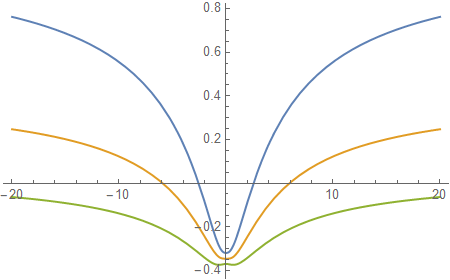
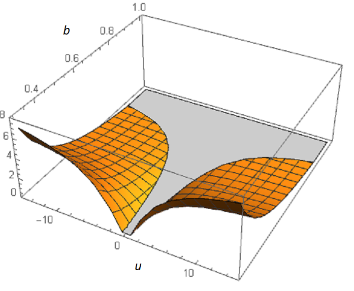
Figure 1: The function $h(\phi(u))$, Eq. (25). Left: $k=1,\ a=0.7,\ b=0.5,\ 0.6,\ 0.7$ (upside down). Right: $k=1,\ a=0.3$, the gray “floor” indicates areas where $h(\phi)<0$. At other values of $a$ the picture is qualitatively similar: $h<0$ near the throat ($u=0$) and remains negative in all space at sufficiently large $b$ but changes its sign and thus exhibits a “trapped ghost” behavior at smaller $b$.

Our next task is to determine the suitable NED Lagrangian ${\mathcal{L}}({\mathcal{F}})$ from the difference of Eqs. (15) and (17). A calculation gives

$${\mathcal{F}}\frac{d{\mathcal{L}}}{d{\mathcal{F}}}=G^{\theta}_{\theta}-G^{t}_{t}=\frac{b^{2}k(2a-1)}{y^{4-a}(2k+y)^{1+a}}.$$ (27)

Since ${\mathcal{F}}=2q^{2}/r^{4}$ and $r^{2}=y^{1-a}(2k+y)^{1+k}$, it is easy to find $d{\mathcal{F}}/{\mathcal{F}}$ in terms of $y$ (and it is now not important that we have put $y=\sqrt{u^{2}+b^{2}}$):

$$\frac{d{\mathcal{F}}}{{\mathcal{F}}}=-\frac{4[y+k(1-a)]}{y(2k+y)},$$ (28)

and therefore we can calculate ${\mathcal{L}}$ as a function of $y$ by integrating the expression

$$\frac{d{\mathcal{L}}}{dy}=\frac{4b^{2}k(1-2a)[y+k(1-a)]}{y^{5-a}(2k+y)^{2+a}},$$ (29)

with the result

$${}{\mathcal{L}}({\mathcal{F}})=\frac{(2a-1)b^{2}(1+2k/y)^{-a}}{(4-a)(3-a)(2-a)(1-a)ak^{4}y^{4}(2k+y)}\bigg{\{}4a^{5}k^{5}-9[-1+(1+2k/y)^{a}]y^{4}(2k+y)$$

$${}\hskip 28.45274pt\ \ +a^{4}(-28k^{5}+6k^{4}y)+4a^{3}k^{3}(17k^{2}-3ky+3y^{2})-2a^{2}(34k^{5}+3k^{4}y-9k^{2}y^{3})$$

$${}\hskip 72.26999pt+6ak(4k^{4}+2k^{3}y-2k^{2}y^{2}+3ky^{3}+3y^{4})\bigg{\}},$$ (30)

where, to get an explicit function of ${\mathcal{F}}$, one should substitute $y=y({\mathcal{F}})$ as a solution to the transcendental equation $y^{2-2a}(y+2k)^{2+2a}=2q^{2}/{\mathcal{F}}$.

A feature of interest is that ${\mathcal{L}}({\mathcal{F}})=0$ in the case $a=1/2$, which means that the regular metric (20) is obtained with only a scalar source, without NED. In fact, it becomes possible because in this case we have $G^{t}_{t}=G^{\theta}_{\theta}$ for the metric (20).

In the general case, the asymptotic behavior of ${\mathcal{L}}({\mathcal{F}})$ at large $|u|$ is

$${\mathcal{L}}({\mathcal{F}})\approx\frac{4(2a-1)b^{2}k}{5|u|^{5}}\ \ {\rm as}\ \ u\to\pm\infty,$$ (31)

A more general picture is illustrated in Fig. 2.

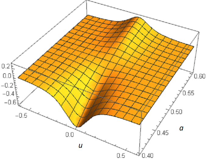
Figure 2: The function ${\mathcal{L}}({\mathcal{F}}(u))$ at $k=1,\ b=0.1$. Its behavior is similar at other values of $b$: it is regular and smooth, it is positive at $a>1/2$, zero at $a=1/2$ and negative at $a<1/2$.

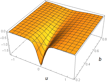
Figure 3: The potential $V(\phi(u))$ for the scalar field (24), (25), with $k=1,\ a=0.5$ (exceptional case). The behavior of $V(\phi)$ turns out to be qualitatively the same in the exceptional and generic cases.

The last quantity to be determined is the potential $V(\phi)$, which can be found, for example, from the radial component (16) of the Einstein equations,

$$V(\phi)=-G^{u}_{u}+A(u)h(\phi)\phi^{\prime}{}^{2}-\dfrac{1}{2}{\mathcal{L}}({\mathcal{F}}).$$ (32)

where we must substitute $G^{u}_{u}$ for the metric (20), $A(u)$ from the same metric, $h$, $\phi$ and ${\mathcal{L}}({\mathcal{F}})$ as determined above. The calculation gives

$$V(\phi)=-\frac{(1-a)b^{2}k}{y^{4-a}(2k+y)^{1+a}}-\dfrac{1}{2}{\mathcal{L}}({\mathcal{F}}),$$ (33)

where ${\mathcal{L}}({\mathcal{F}})$ is given by (III). In the exceptional case $a=1/2$ where the regularized metric (20) is sourced by the scalar field $\phi$ alone, its potential has the form

$$V(\phi)\bigg{|}_{a=1/2}=-\frac{b^{2}k}{2y^{7/2}(2k+y)^{3/2}},$$ (34)

where the substitution $y=b/\cos\phi$ leads to an explicit expression in terms of $\phi$. A more general qualitative behavior of $V(\phi)$ is shown in Fig. 3. At large $|u|$ we have $V(\phi)\sim 1/u^{5}$.

IV Regularized dilatonic black hole

Dilatonic black holes are space-times obtained as special solutions to the Einstein equations with a material source representing of a massless scalar field interacting with an electromagnetic field as described by the action

$$S_{\rm dil}=\dfrac{1}{2}\int\sqrt{-g}\,d^{4}x\big{[}2g^{\mu\nu}\Phi_{,\mu}\Phi_{,\nu}-{\,\rm e}^{2\lambda\Phi}F_{\mu\nu}F^{\mu\nu}\big{]},$$ (35)

where $\lambda$ is a coupling constant. The special solution to be considered can be written with the metric (2) such that [42, 43, 44, 45]

$$A(x)=\Big{(}1-\frac{2k}{x}\Big{)}\Big{(}1+\frac{p}{x}\Big{)}^{-2/(1+\lambda^{2})},\qquad r^{2}(x)=x^{2}\Big{(}1+\frac{p}{x}\Big{)}^{2/(1+\lambda^{2})},$$ (36)

with the scalar ($\Phi$) and electric ($\vec{E}$) fields given by

$$\Phi=-\frac{\lambda}{1+\lambda^{2}}\ln\Big{(}1+\frac{p}{x}\Big{)},\qquad 2{\vec{E}}{}^{2}=-F_{\mu\nu}F^{\mu\nu}=\frac{Q^{2}}{r^{4}(x)}{\,\rm e}^{-4\lambda\Phi},$$ (37)

where $k>0$ and $Q$ (the electric charge) are integration constants, and $p=\sqrt{k^{2}+Q^{2}(1+\lambda^{2})}-k>0$.

Let us focus on the case $\lambda=1$, related to string theory [43, 44]. The metric takes the simple form

$$ds^{2}=\frac{1-2k/x}{1+p/x}dt^{2}-\frac{1+p/x}{1-2k/x}dx^{2}-x(x+p)d\Omega^{2}.$$ (38)

This space-time has the Schwarzschild mass $m=k+p/2=Q^{2}/p$, a horizon at $x=2k$, and a singularity at $x=0$. The global causal structure is the same as that of the Schwarzschild space-time.

As before, let us regularize this space-time by replacing $dx\mapsto du$ and $x\mapsto\sqrt{u^{2}+b^{2}}$, $b>0$:

$$ds^{2}=\frac{1-2k/x}{1+p/x}dt^{2}-\frac{1+p/x}{1-2k/x}du^{2}-x(x+p)d\Omega^{2},\qquad x=\sqrt{u^{2}+b^{2}}.$$ (39)

Evidently, the range of $u$ is $u\in{\mathbb{R}}$, the metric (39) is asymptotically flat at $u\to\pm\infty$ and describes:

(i) if $b<2k$, a regular black hole with two horizons at $u=\pm\sqrt{4k^{2}-b^{2}}$ and a black bounce at $u=0$;

(ii) if $b=2k$, a regular extremal black hole with a single extremal horizon (a black throat [17]) at $u=0$;

(iii) if $b>2k$, a symmetric traversable wormhole with a throat at $u=0$; the throat radius is $r_{\rm th}=\min r(u)=\sqrt{b(p+b)}$.

The metric (39) is not a solution of GR with matter specified by (35) but should be a solution corresponding to (5). Let us determine its particular form. As in the previous section, we can begin with the scalar $\phi$, and quite similarly to Eqs. (22)–(25), we now have

$${}r(u)=\sqrt{x(x+p)},\qquad h(\phi)\phi^{\prime}{}^{2}=-\frac{r^{\prime\prime}}{r}=-\frac{(4b^{2}-p^{2})x^{2}+6b^{2}px+3b^{2}p^{2}}{4x^{4}(x+p)^{2}},$$ (40)

(recall that $x=\sqrt{u^{2}+b^{2}}$, and the prime means $d/du$). Furthermore, using the parametrization freedom of $\phi$, we put again

$${}\phi(u)=\arctan(u/b),\qquad u=b\tan\phi,\qquad$$ (41)

$${}\ \Rightarrow\ \ h(\phi)=-\frac{(4b^{2}-p^{2})x^{2}+6b^{2}px+3b^{2}p^{2}}{4b^{2}(x+p)^{2}},$$ (42)

where, according to (41), we should substitute $x=b/\cos\phi$. As $u\to 0$ and $u\to\pm\infty$, $h(\phi)$ behaves as follows:

$$h(\phi)\Big{|}_{u\to 0}\to-\frac{2b+p}{2(b+p)},\qquad h(\phi)\Big{|}_{u\to\infty}\to\frac{p^{2}-4b^{2}}{4b^{2}}.$$ (43)

At $u=0$ we have $h<0$, corresponding to a phantom $\phi$ field. At large $u$, it turns out that the $\phi$ field is canonical ($h>0$) at $b<2p$ and phantom at larger values of $b$. Thus at sufficiently small values of the regularizing parameter $b$, we again meet a “trapped ghost” scalar as a source of the geometry, see Fig. 4.

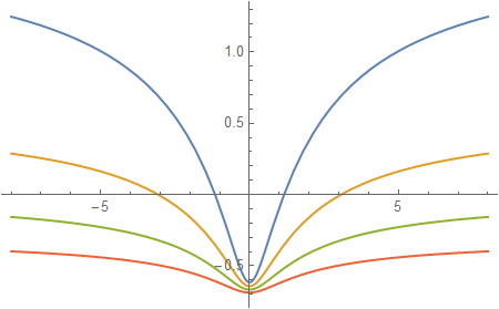
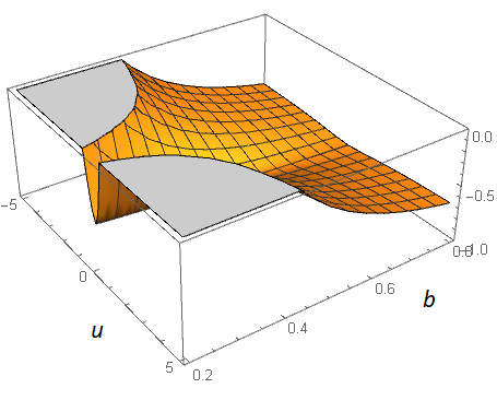
Figure 4: The function $h(\phi(u))$, Eq. (42), with $p=1,\ b=0.3,\ 0.4,\ 0.5,\ 0.6$ (left, upside down), and for a range of $b$ (right), where gray tops show regions with $h(\phi(u))>0$. At sufficiently small values of $b$ at given $p$, the scalar $\phi$ has a trapped-ghost nature.

Next, the difference of Eqs. (15) and (17) allows for finding ${\mathcal{L}}({\mathcal{F}})$:

$${}\frac{d{\mathcal{L}}}{dx}=\frac{1}{{\mathcal{F}}}\frac{d{\mathcal{F}}}{dx}(G^{\theta}_{\theta}-G^{t}_{t})=-\frac{2(p+2x)}{x^{5}(p+x)^{4}}\Big{(}b^{2}\left[k(p^{2}+2px+3x^{2})+px^{2}\right]+p(2k+p)x^{3}\Big{)},$$ (44)

$${}{\mathcal{L}}({\mathcal{F}})=\frac{2}{p^{5}}[b^{2}(k+2p)-2p^{2}(2k+p)]\ln\frac{x+p}{x}$$

$${}\hskip 28.45274pt-\frac{1}{6p^{5}x^{4}(p+x)^{3}}\Big{\{}-4p^{3}x^{3}(2k+p)(3p+2x)(p^{2}+3px+3x^{2})$$

$${}\hskip 28.45274pt+b^{2}p\big{[}-3kp^{6}-9kp^{5}x-3p^{4}(5k+2p)x^{2}+(k+2p)(3p^{3}x^{3}+22p^{2}x^{4}+30px^{5}+12x^{6})\big{]}\Big{\}},$$ (45)

where, to really obtain ${\mathcal{L}}$ as a function of ${\mathcal{F}}$, one should substitute $x$ as a solution to the quartic equation $x^{2}(x+p)^{2}=2q^{2}/{\mathcal{F}}$. Thus the expression of ${\mathcal{L}}({\mathcal{F}})$ is quite complicated. Still it is clear that it is a regular function, and we illustrate its behavior in terms of $x$ for some examples of the parameter values in Fig. 5.

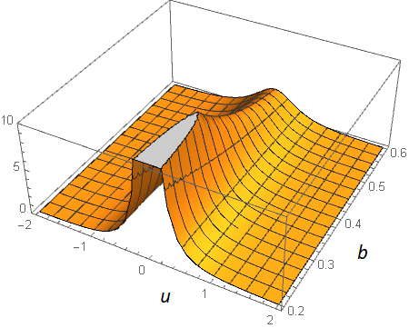
Figure 5: The NED Lagrangian function ${\mathcal{L}}({\mathcal{F}}(u))$, Eq. (IV), at $k=p=1$. At other values of the parameters the behavior of ${\mathcal{L}}({\mathcal{F}}(u))$ is qualitatively the same.

Note that at large $x$ we have

$${\mathcal{L}}({\mathcal{F}})\approx\frac{p(2k+p)}{x^{4}}\approx\frac{2Q^{2}}{r^{4}}=\frac{Q^{2}}{q^{2}}{\mathcal{F}},$$ (46)

it exhibits a Maxwell asymptotic behavior. Recall that $Q$ is the electric charge in the dilatonic black hole (38), (37) with $\lambda=1$, which has nothing to do with the magnetic charge $q$ used in the NED model that supports the regularized solution.

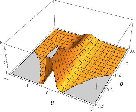
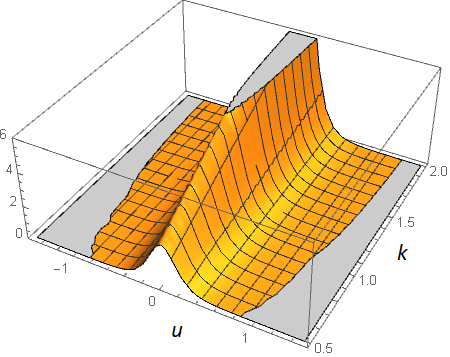
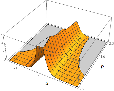
Figure 6: The potential $V(\phi(u))$, Eq. (47), for the scalar field (41), (42) with $k=1,\ p=1$ and different $b$ (left), $p=1,\ b=0.3$, and different $k$ (middle), and $k=1,\ b=0.3$, and different $p$ (right). Gray bottoms show the regions where $V(\phi(u))<0$.

The scalar field potential $V(\phi)$ is again obtained according to (32) and reads

$${}V(\phi)=\frac{p(2k+p)x^{3}+b^{2}\big{[}px^{2}+2k(p^{2}+2px+2x^{2})\big{]}}{2x^{4}(p+x)^{3}}-\dfrac{1}{2}{\mathcal{L}}({\mathcal{F}}),$$ (47)

where ${\mathcal{L}}({\mathcal{F}})$ is given by (IV), and, as before, $x=b/\cos\phi$. At large $x$ we have $x\approx|u|\approx r(u)$, and $V(\phi)$ behaves as

$$V(\phi)\approx\frac{8b^{2}k+b^{2}p-2kp^{2}-p^{3}}{10|u|^{5}}.$$ (48)

The behavior of $V$ in the whole space is illustrated in Fig. 6.

V Concluding remarks

In the previous studies of spherically symmetric black-bounce space-times, the SV regularization trick was applied to the spherical radius $r$ in the form $r=\sqrt{u^{2}+b^{2}}$, even though some general reasoning used an arbitrary function $r(u)$ [19, 53] (or $\Sigma(r)$ in their notation). Consequently, the expression $r^{\prime\prime}/r=b^{2}/r^{4}$, determining the sign of $h(\phi)$ (see (14) and (18)), is everywhere positive, making $h(\phi)<0$ in the whole space, and a scalar field $\phi$, able to support the corresponding regular metric, is inevitably phantom. Unlike that, in our examples (III) and (38) it is more reasonable to make the corresponding replacement not in $r$ but in a parameter whose zero value leads to a singularity. As a result, $r^{\prime\prime}/r$ is, in general, not everywhere nonnegaitive, and the field $\phi$ supporting the model is then necessarily of trapped-ghost nature, which is a new feature of this kind of models.

It is not surprising that a general static, spherically symmetric metric (2), containing two arbitrary functions $A(x)$ and $r(x)$ can be supported by a matter source with also two arbitrary functions, $V(\phi)$ and ${\mathcal{L}}({\mathcal{F}})$, but the regularization is here slightly complicated by the necessity of trapped-ghost fields.

As to the NED source of the same models, it cannot affect the NEC violation related to $r^{\prime\prime}/r>0$ due to the equality $T^{t}_{t}=T^{x}_{x}$, see (8) and (12). If this equality holds for a full SET, a regular minimum of $r(x)$ is impossible, therefore static, spherically symmetric wormholes with a purely NED source cannot exist: there can be either magnetic black holes or solitons with a regular center or dynamic wormholes existing in a finite period of time, see, e.g., [54, 55] and references therein.

By construction, the regularized configurations considered here are ${\mathbb{Z}}_{2}$-symmetric with respect to the minimum-$r$ sphere $u=0$. Therefore, black holes with a single horizon, like the Schwarzschild one or the dilatonic one given by (36), turn into regular black holes with two horizons (at least for small values of the regularization parameter $b$); black holes with two horizons like the Reissner-Nordström ones turn into those with four horizons, etc. Thus the regularization substantially complicates the global causal structure of space-times, as demonstrated, in particular, by Carter-Penrose diagrams for three- and four-horizon black holes presented in [17] and occupying the whole plane plus a countable set of overlappings. It is also clear that thus regularized black hole metrics cannot have any kind of scalar field as their only source since it would violate the global structure theorem [56] from which it follows that an asymptotically flat static, spherically symmetric configuration in GR with a scalar source cannot contain more than one horizon. Unlike that, regularization of a metric with a naked singularity leads to a wormhole whose source can be a scalar field alone, and such an example has been really obtained here with the metric (III) in the special case $a=1/2$. A single scalar field source for an arbitrary metric (2) can be obtained (though under some resrictions) if we consider scalar-tensor theories instead of GR [58], due to arbitrariness of the nonminimal coupling function $f(\phi)$ in the Lagrangian.

A problem of interest is the stability of regularized space-times, and it is important to mention that the stability properties of a given geometry can be different, depending on the dynamics of the sources of this geometry. For example, the simplest Ellis wormhole [57, 50] can be stable or unstable depending on the nature of its source — a phantom scalar, a kind of perfect fluid or a k-essence field [59, 60, 61]. We can also recall that Fisher’s solution (III) was found to be unstable due to its behavior near its naked singularity [62], and it can be a subject of a further study to find out how this result may change if the singularity is replaced by a wormhole throat and there is a trapped-ghost scalar field as a source.

Acknowledgment

I am grateful to Manuel E. Rodrigues for pointing out an error in the previous version of the paper.

References

- [1] D. Malafarina, Classical collapse to black holes and quantum bounces: A review, Universe 3, 48 (2017).
- [2] H. M. Haggard and C. Rovelli, Black hole fireworks: quantum-gravity effects outside the horizon, spark black to white hole tunneling. Phys. Rev. D 92, 104020 (2015).
- [3] L. Modesto, Space-time structure of loop quantum black hole. Int. J. Theor. Phys. 49, 1649 (2010).
- [4] J. G. Kelly, R. Santacruz, and E. Wilson-Ewing, Black hole collapse and bounce in effective loop quantum gravity, arXiv: 2006.09325.
- [5] J.B. Achour, S. Brahma, S. Mukohyama, and J.-P. Uzan, Towards consistent black-to-white hole bounces from matter collapse, JCAP 2020, 20 (2020).
- [6] R.G. Daghigh, M.D. Green, J.C. Morey, and G. Kunstatter, Perturbations of a single-horizon regular black hole, arXiv: 2009.02367.
- [7] A. Ashtekar and J. Olmedo, Properties of a recent quantum extension of the Kruskal geometry, arXiv: 2005.02309.
- [8] C. Bambi, D. Malafarina, and L. Modesto, Non-singular quantum-inspired gravitational collapse. Phys. Rev. D 88, 044009 (2013).
- [9] K. A. Bronnikov, S. V. Bolokhov, and M. V. Skvortsova, Matter accretion versus semiclassical bounce in Schwarzschild interior, Universe 6, 178 (2020); arXiv: 2009.06330.
- [10] A. Simpson and M. Visser, Black bounce to traversable wormhole, JCAP 02, 042 (2019).
- [11] K. A. Bronnikov and J. C. Fabris, Regular phantom black holes, Phys. Rev. Lett. 96, 251101 (2006).
- [12] K. A. Bronnikov, V. N. Melnikov and H. Dehnen, Regular black holes and black universes, Gen. Rel. Grav. 39, 973 (2007).
- [13] S. V. Bolokhov, K. A. Bronnikov and M. V. Skvortsova, Magnetic black universes and wormholes with a phantom scalar, Class. Quantum Gravity 29, 245006 (2012).
- [14] G. Clement, J. C. Fabris and M.E. Rodrigues, Phantom black holes in Einstein-Maxwell-dilaton theory, Phys. Rev. D 79, 064021 (2009).
- [15] M. Azreg-Ainou, G. Clement, J. C. Fabris and M. E. Rodrigues, Phantom black holes and sigma models, Phys. Rev. D 83, 124001 (2011).
- [16] K. A. Bronnikov. Scalar fields as sources for wormholes and regular black holes, Particles 2018, 1, 5; arXiv: 1802.00098.
- [17] K. A. Bronnikov and R. K. Walia, Field sources for Simpson-Visser space-times, Phys. Rev. D 105, 044039 (2022); arXiv: 2112.13198.
- [18] E. Franzin, S. Liberati, J. Mazza, A. Simpson and M. Visser, Charged black-bounce spacetimes, JCAP 07, 036 (2021).
- [19] F. S. N. Lobo, M. E. Rodrigues, M. V .d.S. Silva, A. Simpson, and M. Visser, Novel black-bounce spacetimes: wormholes, regularity, energy conditions, and causal structure, Phys. Rev. D 103, 084052 (2021).
- [20] J. Mazza, E. Franzin and S. Liberati, A novel family of rotating black hole mimickers, JCAP 04, 082 (2021).
- [21] Z. Xu and M. Tang, Rotating spacetime: black-bounces and quantum deformed black hole, Eur. Phys. J. C 81, 863 (2021).
- [22] R. Shaikh, K. Pal, K. Pal and T. Sarkar, Constraining alternatives to the Kerr black hole, Mon. Not. Roy. Astron. Soc. 506, 1229 (2021).
- [23] Y. Yang, D. Liu, Z. Xu, Y. Xing, S. Wu and Z. W. Long, Echoes of novel black-bounce spacetimes, Phys. Rev. D 104, 104021 (2021).
- [24] M. S. Churilova and Z. Stuchlik, Ringing of the regular black-hole/wormhole transition, Class. Quant. Grav. 37, 075014 (2020).
- [25] M. Guerrero, G. J. Olmo, D. Rubiera-Garcia and D. S. C. Gómez, Shadows and optical appearance of black bounces illuminated by a thin accretion disk, JCAP 08, 036 (2021).
- [26] N. Tsukamoto, Gravitational lensing by two photon spheres in a black-bounce spacetime in strong deflection limits, Phys. Rev. D 104, 064022 (2021).
- [27] S. U. Islam, J. Kumar and S. G. Ghosh, Strong gravitational lensing by rotating Simpson-Visser black holes, JCAP 10, 013 (2021).
- [28] X. T. Cheng and Y. Xie, Probing a black-bounce, traversable wormhole with weak deflection gravitational lensing, Phys. Rev. D 103, 064040 (2021).
- [29] K. A. Bronnikov and R. A. Konoplya, Echoes in brane worlds: Ringing at a black hole-wormhole transition, Phys. Rev. D 101 064004 (2020); arXiv: 1912.05315.
- [30] N. Tsukamoto, Gravitational lensing in the Simpson-Visser black-bounce spacetime in a strong deflection limit, Phys. Rev. D 103, 024033 (2021).
- [31] Haroldo C. D. Lima Junior, Luis C. B. Crispino, Pedro V. P. Cunha, and Carlos A. R. Herdeiro, Can different black holes cast the same shadow? Phys. Rev. D 103, 084040 (2021); arXiv: 2102.07034.
- [32] J. R. Nascimento, A. Y. Petrov, P. J. Porfirio and A. R. Soares, Gravitational lensing in black-bounce spacetimes, Phys. Rev. D 102, 044021 (2021).
- [33] Edgardo Franzin, Stefano Liberati, Jacopo Mazza, Ramit Dey, and Sumanta Chakraborty, Scalar perturbations around rotating regular black holes and wormholes: quasi-normal modes, ergoregion instability and superradiance, Phys. Rev. D 105, 124051 (2022); arXiv: 2201.01650.
- [34] Pedro Cañate, Black-bounces as magnetically charged phantom regular black holes in Einstein-nonlinear electrodynamics gravity coupled to a self-interacting scalar field, Phys. Rev. D 106, 024031 (2022); arXiv: 2202.02303.
- [35] Leonardo Chataignier, Alexander Yu. Kamenshchik, Alessandro Tronconi, and Giovanni Venturi, Regular black holes, universes without singularities, and phantom-scalar field transitions, arXiv: 2208.02280.
- [36] H. Kroger, G. Melkonian and S. G. Rubin, Cosmological dynamics of scalar field with non-minimal kinetic term, Gen. Rel. Grav. 36, 1649 (2004).
- [37] K. A. Bronnikov and S. V. Sushkov, Trapped ghosts: a new class of wormholes, Class. Quantum Grav. 27, 095022 (2010).
- [38] K. A. Bronnikov and E. V. Donskoy, Black universes with trapped ghosts. Grav. Cosmol. 17 (1), 31 (2011); arXiv: 1110.6030.
- [39] K. A. Bronnikov. Trapped ghosts as sources for wormholes and regular black holes. The stability problem. In: Wormholes, Warp Drives and Energy Conditions, ed. F.S.N. Lobo, Springer, 2017, p. 137-160.
- [40] I. Z. Fisher, Scalar mesostatic field with regard for gravitational effects, J. Eksp. Teor. Fiz. 18, 636 (1948); gr-qc/9911008 (translation into English).
- [41] A. I. Janis, E. T. Newman, and J. Winicour, Reality of the Schwarzschild singularity, Phys. Rev. Lett. 20, 878 (1968).
- [42] K. A. Bronnikov and G. N. Shikin, On interacting fields in general relativity, Russ. Phys. J. 20, 1138–1143 (1977).
- [43] G. W. Gibbons and K.-i. Maeda, Black holes and membranes in higher dimensional theories with dilaton fields, Nucl. Phys. B 298, 741 (1988).
- [44] D. Garfinkle, G.T. Horowitz, and A. Strominger, Charged black holes in string theory, Phys. Rev. D 43, 3140 (1991). [Erratum: Phys. Rev. D 45, 3888 (1992)].
- [45] K.A. Bronnikov. Spherically symmetric solutions in D-dimensional dilaton gravity, Grav. Cosmol. 1, 67 (1995).
- [46] H. Nilles, Supersymmetry, supergravity and particle physics, Phys. Rep. 110, 1 (1984).
- [47] N. Khviengia, Z. Khviengia, H. Lü, and C. N. Pope, Towards a field theory of F-theory, Class. Quantum Grav. 15, 759 (1998); hep-th/9703012.
- [48] K. A. Bronnikov and S. G. Rubin. Black Holes, Cosmology, and Extra Dimensions (2nd edition, World Scientific, 2021).
- [49] O. Bergmann and R. Leipnik, Space-time structure of a static spherically symmetric scalar field, Phys. Rev. 107, 1157 (1957).
- [50] K. A. Bronnikov, Scalar-tensor theory and scalar charge, Acta Phys. Pol. B 4, 251 (1973).
- [51] K. A. Bronnikov, J.C. Fabris, N. Pinto-Neto, and M. E. Rodrigues, Cold black holes in the Einstein-scalar field system, gr-qc/0604055.
- [52] Kunal Pal, Kuntal Pal, Pratim Roy, and Tapobrata Sarkar, Regularising the JNW and JMN naked singularities, arXiv: 2206.11764.
- [53] Alex Simpson, From black bounce to traversable wormhole, and beyond, arXiv: 2110.05657.
- [54] K.A. Bronnikov, Regular magnetic black holes and monopoles from nonlinear electrodynamics, Phys. Rev. D 63, 044005 (2001).
- [55] K. A. Bronnikov, Nonlinear electrodynamics, regular black holes and wormholes, Int. J. Mod. Phys. D 27, 1841005 (2018).
- [56] K. A. Bronnikov, Spherically symmetric false vacuum: No-go theorems and global structure, Phys. Rev. D 64, 064013 (2001).
- [57] H. G. Ellis, Ether flow through a drainhole: a particle model in general relativity, J. Math. Phys. 14, 104 (1973).
- [58] K. A. Bronnikov, Kodir Badalov, and Rustam Ibadov, Arbitrary static, spherically symmetric space-times as solutions of scalar-tensor gravity, Grav. Cosmol. 29, 43 (2023); arXiv: 2212.04544.
- [59] J.A. González, F.S. Guzmán and O. Sarbach, Instability of wormholes supported by a ghost scalar field. I. Linear stability analysis, Class. Quantum Grav. 26, 015010 (2009); arXiv: 0806.0608.
- [60] K. A. Bronnikov, L. N. Lipatova, I. D. Novikov, and A. A. Shatskiy, Example of a stable wormhole in general relativity. Grav. Cosmol. 19, 269 (2013).
- [61] Kirill A. Bronnikov, Vinicius A. G. Barcellos, Laura P. de Carvalho, and Júlio C. Fabris, The simplest wormhole in Rastall and k-essence theories. Eur. Phys. J. C 81, 395 (2021); arXiv: 2102.10797.
- [62] K. A. Bronnikov and A. V. Khodunov. Scalar field and gravitational instability, Gen. Rel. Grav. 11, 13 (1979).