POD-ROMs for incompressible flows including snapshots of the temporal derivative of the full order solution

Bosco García-Archilla Departamento de Matemática Aplicada II, Universidad de Sevilla, Sevilla, Spain, (), \fundingThe research of Bosco García-Archilla has been supported by Spanish MCINYU under grants PGC2018-096265-B-I00 and PID2019-104141GB-I00. bosco@esi.us.es    Volker John Weierstrass Institute for Applied Analysis and Stochastics, Leibniz Institute in Forschungsverbund Berlin e. V. (WIAS), Mohrenstr. 39, 10117 Berlin, Germany. Freie Universität of Berlin, Department of Mathematics and Computer Science, Arnimallee 6, 14195 Berlin, Germany, (). john@wias-berlin.de    Julia Novo Departamento de Matemáticas, Universidad Autónoma de Madrid, Spain, (), \fundingThe research of Julia Novo has been supported by Spanish MINECO under grants PID2019-104141GB-I00 and VA169P20. julia.novo@uam.es
Abstract

In this paper we study the influence of including snapshots that approach the velocity time derivative in the numerical approximation of the incompressible Navier–Stokes equations by means of proper orthogonal decomposition (POD) methods. Our set of snapshots includes the velocity approximation at the initial time from a full order mixed finite element method (FOM) together with approximations to the time derivative at different times. The approximation at the initial velocity can be replaced by the mean value of the velocities at the different times so that implementing the method to the fluctuations, as done mostly in practice, only approximations to the time derivatives are included in the set of snapshots. For the POD method we study the differences between projecting onto L2superscript𝐿2L^{2} and H1superscript𝐻1H^{1}. In both cases, pointwise in time error bounds are proved. Including grad-div stabilization both in the FOM and POD methods, error bounds with constants independent of inverse powers of the viscosity are obtained.

keywords:
incompressible Navier–Stokes equations; proper orthogonal decomposition (POD); reduced order models (ROMs); snapshots of the temporal derivative of the full order solution; grad-div stabilization; robust pointwise in time estimates
{AMS}

65M12, 65M15, 65M60

1 Introduction

It is well known that the computational cost of direct numerical simulations, also called full order methods (FOMs), can be reduced by using reduced order models (ROMs). In this paper, we study ROMs based on proper orthogonal decomposition (POD) methods, so-called POD-ROMs. The computation of the reduced basis uses solutions of a FOM, so-called snapshots.

We study incompressible flow problems that are modeled by means of the incompressible Navier–Stokes equations

(1) 𝒖tνΔ𝒖+(𝒖)𝒖+p=𝒇in (0,T]×Ω,𝒖=0in (0,T]×Ω,subscript𝒖𝑡𝜈Δ𝒖𝒖𝒖𝑝𝒇in 0𝑇Ω𝒖0in 0𝑇Ω\begin{array}[]{rcll}\boldsymbol{u}_{t}-\nu\Delta\boldsymbol{u}+(\boldsymbol{u}\cdot\nabla)\boldsymbol{u}+\nabla p&=&\boldsymbol{f}&\text{in }\ (0,T]\times\Omega,\\ \nabla\cdot\boldsymbol{u}&=&0&\text{in }\ (0,T]\times\Omega,\end{array}

in a bounded domain ΩdΩsuperscript𝑑\Omega\subset{\mathbb{R}}^{d}, d{2,3}𝑑23d\in\{2,3\}, with initial condition 𝒖(0)=𝒖0𝒖0superscript𝒖0\boldsymbol{u}(0)=\boldsymbol{u}^{0}. In (1), 𝒖𝒖\boldsymbol{u} is the velocity field, p𝑝p the kinematic pressure, ν>0𝜈0\nu>0 the kinematic viscosity coefficient, and 𝒇𝒇\boldsymbol{f} represents the accelerations due to external body forces acting on the fluid. The Navier–Stokes equations (1) have to be complemented with boundary conditions. For simplicity, we only consider homogeneous Dirichlet boundary conditions 𝒖=𝟎𝒖0\boldsymbol{u}=\boldsymbol{0} on [0,T]×Ω0𝑇Ω[0,T]\times\partial\Omega.

This paper studies the impact of including approximations of the temporal derivative of the velocity in the set of snapshots. The idea consists in taking, in addition to the mixed finite element approximation to the velocity at the initial time, {𝒖h(t0)}subscript𝒖subscript𝑡0\left\{\boldsymbol{u}_{h}(t_{0})\right\}, the time derivatives of the mixed finite element approximations, {𝒖h,t(tj)}subscript𝒖𝑡subscript𝑡𝑗\left\{\boldsymbol{u}_{h,t}(t_{j})\right\}. These temporal derivatives can be easily computed using the right-hand side of the mixed finite element Galerkin equation (see Remark 2 below). In the present paper we follow an idea presented in the recent paper [25] in which it is shown that there is no need to include in the set of snapshots other than one approximation to the velocity at a fixed time, instead of the full set {𝒖h(tj)}j=0Msuperscriptsubscriptsubscript𝒖subscript𝑡𝑗𝑗0𝑀\left\{\boldsymbol{u}_{h}(t_{j})\right\}_{j=0}^{M} as it is usually done in the literature. The numerical analysis in [25] is carried out for the heat equation and with difference quotients, {(𝒖h(tj)𝒖h(tj1)/(tjtj1)}\left\{(\boldsymbol{u}_{h}(t_{j})-\boldsymbol{u}_{h}(t_{j-1})/(t_{j}-t_{j-1})\right\}, approaching the time derivative. In the present paper we consider instead the Galerkin time derivatives although the analysis for the difference quotients case is essentially the same (or even simpler). Actually, in practice, any approximation to the time derivative can work equally well. We also prove that the snapshot at the initial value can be replaced by the mean value 𝒖¯h=(M+1)1j=0M𝒖h(tj)subscript¯𝒖superscript𝑀11superscriptsubscript𝑗0𝑀subscript𝒖subscript𝑡𝑗\overline{\boldsymbol{u}}_{h}=(M+1)^{-1}\sum_{j=0}^{M}\boldsymbol{u}_{h}(t_{j}), which can be more efficient in the numerical simulations. It is standard to apply the POD method to the fluctuations {𝒚h(tj)}j=0M={𝒖h(tj)𝒖¯h}j=0Msuperscriptsubscriptsubscript𝒚subscript𝑡𝑗𝑗0𝑀superscriptsubscriptsubscript𝒖subscript𝑡𝑗subscript¯𝒖𝑗0𝑀\left\{\boldsymbol{y}_{h}(t_{j})\right\}_{j=0}^{M}=\left\{\boldsymbol{u}_{h}(t_{j})-\overline{\boldsymbol{u}}_{h}\right\}_{j=0}^{M} that have vanishing mean by definition. Then, with the method we propose only approximations to the derivatives are needed in this case.

Several works in the literature have already studied the subject of increasing the set of snapshots with approximations to the time derivatives. However, apart from [25], all of them include as snapshots the set of the approximations at different times, instead of only one snapshot. Also, starting with the pioneering paper [23], most of these papers include a different type of approximation than considered in this paper, namely difference quotients. In particular, to the best of our knowledge, this is the first paper that studies the inclusion of the temporal derivatives of the mixed finite element velocity approximations in order to generate the reduced order basis for the incompressible Navier–Stokes equations. With this more general setting we can deduce that in practice any approximation to the time derivative produces essentially the same results.

The initial motivation for investigating a different approximation than difference quotients in the set of snapshots is that the results for difference quotients are ambivalent. On the one hand, from the theoretical point of view, the inclusion of the difference quotients possesses some advantages. First of all, it allows to prove optimal error bounds for the POD-ROM when the POD basis functions are based on the projection onto the Hilbert space X=H01(Ω)d𝑋superscriptsubscript𝐻01superscriptΩ𝑑X=H_{0}^{1}(\Omega)^{d}, see [23, 17, 30]. In this way, the standard finite element error analysis is mimicked, in which the Ritz or Stokes projection is used to split the error in a projection error and a discrete remainder. It was observed that if the POD basis functions are based on the projection onto the Hilbert space X=L2(Ω)d𝑋superscript𝐿2superscriptΩ𝑑X=L^{2}(\Omega)^{d}, the difference quotients are not needed to prove optimal error bounds in certain norms, see [4, 17, 30, 26]. However, as pointed out in [21], even in this case, the inclusion of the difference quotients allows to get pointwise estimates in time that generally cannot be proved if there are no difference quotients in the set of snapshots. On the other hand, from the numerical point of view, it is not clear that the difference quotients should be included in the actual simulations with the POD-ROM. In fact, it is reported in [20, 19] that the POD-ROM without the difference quotients performs considerably better than with the difference quotients.

Trying to keep the theoretical advantages of including approximations of the temporal derivative of the velocity in the set of snapshots but relaxing their drawbacks in practical simulations, we study in this paper, both theoretically and numerically, the inclusion of time derivatives of the discrete velocity. As in [25], our approach has half the number of snapshots as in the standard POD finite quotient approach. Also, as in the difference quotient case, we are able to get pointwise in time estimates using as projecting space X=H01(Ω)d𝑋superscriptsubscript𝐻01superscriptΩ𝑑X=H_{0}^{1}(\Omega)^{d} and L2(Ω)dsuperscript𝐿2superscriptΩ𝑑L^{2}(\Omega)^{d}. To this end, we follow [25, Lemma 3.3] (see also [21, Lemma 3.6]) to prove that the X𝑋X-norm of a function at any point in time (let’s say tjsubscript𝑡𝑗t_{j}) is bounded in terms of the X𝑋X-norm of the value at t0subscript𝑡0t_{0} plus the mean values of its time derivative taken in a time interval (let’s say {t0,t1,,tM}subscript𝑡0subscript𝑡1subscript𝑡𝑀\left\{t_{0},t_{1},\ldots,t_{M}\right\}, up to an error that tends to zero with the length of the time step. From the numerical point of view, including the snapshots of the time derivatives avoids the potential problem of performing badly conditioned operations in the computation of the snapshots like {(𝒖h(tj)𝒖h(tj1))/(tjtj1)}subscript𝒖subscript𝑡𝑗subscript𝒖subscript𝑡𝑗1subscript𝑡𝑗subscript𝑡𝑗1\left\{(\boldsymbol{u}_{h}(t_{j})-\boldsymbol{u}_{h}(t_{j-1}))/(t_{j}-t_{j-1})\right\} because both numerator and denominator may suffer from numerical cancellation. Finally, we mimic model reduction ideas coming from dynamical systems, where using snapshots from the time derivative is a more common approach, see for example [22].

For the error analysis in the present paper, instead of considering a concrete fully discrete scheme from which the values {𝒖h(tj)}subscript𝒖subscript𝑡𝑗\left\{\boldsymbol{u}_{h}(t_{j})\right\} are taken, we consider a continuous-in-time method, which has some advantages. In practice, one always computes the snapshots with a fully discrete method but the error analysis based on the continuous-in-time method holds for any time integrator used in the FOM. With this approach one can use different time steps for the FOM, which produces the snapshots, and for the POD-ROM method. Our error analysis takes into account the temporal error coming from the POD-ROM. The error analysis of the present paper can be easily adapted to include the case in which the snapshots are computed with a fully discrete method. Errors with respect the fully discrete approximations can be expressed in terms of errors with respect the continuous-in-time approximation (estimated in the present paper) and further terms depending on the error of the fully discrete approximation with respect to the continuous-in-time one, for which there are already estimates in the literature.

Finally, following [26], we analyze the case in which stabilized approximations are computed both for the FOM and the POD-ROM. More precisely, the considered finite element method is based on a Galerkin discretization plus grad-div stabilization with pairs of inf-sup stable elements, and, as in references [26, 12], for the POD-ROM we also use grad-div stabilization. In this way, the constants in the error bounds for the snapshots do not depend explicitly on inverse powers of the viscosity, i.e., they do not blow up for small viscosity coefficients, see [9]. Adapting the results from [26], the same holds for the error bounds of the POD-ROM. The importance of such so-called robust methods is stated in the survey [11]: In the case of small viscosity coefficients and coarse grids, only robust estimates provide useful information about the behavior of a numerical method on coarse grids if the analytic solution is smooth. In reference [12] a POD scheme with data assimilation was analyzed. In the method of [12], grad-div stabilization was added to the POD method, but the plain Galerkin method was used for the FOM so that the final error bounds depend on inverse powers of the viscosity. As opposed to the present paper, neither in reference [26] nor in [12], snapshots approaching the time derivative are included and no pointwise estimates are proved.

In the numerical studies, we compare the different approaches obtained by taking X=H01(Ω)d𝑋superscriptsubscript𝐻01superscriptΩ𝑑X=H_{0}^{1}(\Omega)^{d} and X=L2(Ω)d𝑋superscript𝐿2superscriptΩ𝑑X=L^{2}(\Omega)^{d} in combination with one of the following sets: the set of snapshots at different times, the set of difference quotients, and the set of Galerkin time derivatives. We cannot deduce from these studies that any of the approaches is much better than the other ones and the necessary comprehensive numerical studies are outside the scope of this paper, which is a rigorous numerical analysis from which interesting properties and sharp bounds for the different methods can be deduced.

The paper is organized as follows. In Section 2 we state some preliminaries and notations. The POD method and some a priori bounds for the projection of the FOM approximation onto the POD space are shown in Section 3. The analysis of the POD method is included in Section 4 with a first subsection for the case X=H01(Ω)d𝑋superscriptsubscript𝐻01superscriptΩ𝑑X=H_{0}^{1}(\Omega)^{d} and a second one for the case X=L2(Ω)d𝑋superscript𝐿2superscriptΩ𝑑X=L^{2}(\Omega)^{d}. As stated above, Section 5 is devoted to study the performance of the methods with some numerical experiments. Finally, we have included an appendix in which we get robust bounds for the second time derivative of the FOM approximation in some norms, since this time derivative appears in our bounds in the a priori error analysis.

2 Preliminaries and notations

Standard symbols will be used for Lebesgue and Sobolev spaces, with the usual convention that Ws,2(Ω)=Hs(Ω)superscript𝑊𝑠2Ωsuperscript𝐻𝑠ΩW^{s,2}(\Omega)=H^{s}(\Omega), s1𝑠1s\geq 1. The inner product in L2(Ω)dsuperscript𝐿2superscriptΩ𝑑L^{2}(\Omega)^{d}, d1𝑑1d\geq 1, is denoted by (,)(\cdot,\cdot), and the corresponding norm by 0\|\cdot\|_{0}.

The following Sobolev imbeddings [1] will be used in the analysis: For q[1,)𝑞1q\in[1,\infty), there exists a constant C=C(Ω,q)𝐶𝐶Ω𝑞C=C(\Omega,q) such that

(2) vLqCvWs,q,1q1qsd>0,q<,vWs,q(Ω)d.formulae-sequenceformulae-sequencesubscriptnorm𝑣superscript𝐿superscript𝑞𝐶subscriptnorm𝑣superscript𝑊𝑠𝑞1superscript𝑞1𝑞𝑠𝑑0formulae-sequence𝑞𝑣superscript𝑊𝑠𝑞superscriptΩ𝑑\|v\|_{L^{q^{\prime}}}\leq C\|v\|_{W^{s,q}},\,\,\quad\frac{1}{q^{\prime}}\geq\frac{1}{q}-\frac{s}{d}>0,\quad q<\infty,\quad v\in W^{s,q}(\Omega)^{d}.

We will denote by Cpsubscript𝐶𝑝C_{p} the constant in the Poincaré inequality

(3) 𝒗0Cp𝒗0,𝒗H01(Ω)d.formulae-sequencesubscriptnorm𝒗0subscript𝐶𝑝subscriptnorm𝒗0𝒗superscriptsubscript𝐻01superscriptΩ𝑑\|\boldsymbol{v}\|_{0}\leq C_{p}\|\nabla\boldsymbol{v}\|_{0},\quad\boldsymbol{v}\in H_{0}^{1}(\Omega)^{d}.

The following inequality can be found in [18, Remark 3.35]

(4) 𝒗0𝒗0,𝒗H01(Ω)d.formulae-sequencesubscriptnorm𝒗0subscriptnorm𝒗0𝒗superscriptsubscript𝐻01superscriptΩ𝑑\|\nabla\cdot\boldsymbol{v}\|_{0}\leq\|\nabla\boldsymbol{v}\|_{0},\quad\boldsymbol{v}\in H_{0}^{1}(\Omega)^{d}.

Let us denote by 𝑽=H01(Ω)d𝑽superscriptsubscript𝐻01superscriptΩ𝑑{\boldsymbol{V}}=H_{0}^{1}(\Omega)^{d} and Q=L02(Ω)={qL2(Ω)(q,1)=0}𝑄superscriptsubscript𝐿02Ωconditional-set𝑞superscript𝐿2Ω𝑞10Q=L_{0}^{2}(\Omega)=\{q\in L^{2}(\Omega)\ \mid\ (q,1)=0\}.

Let 𝒯h=(σjh,ϕjh)jJhsubscript𝒯subscriptsuperscriptsubscript𝜎𝑗superscriptsubscriptitalic-ϕ𝑗𝑗subscript𝐽\mathcal{T}_{h}=(\sigma_{j}^{h},\phi_{j}^{h})_{j\in J_{h}}, h>00h>0, be a family of partitions of Ω¯¯Ω\overline{\Omega}, where hh denotes the maximum diameter of the mesh cells σjh𝒯hsuperscriptsubscript𝜎𝑗subscript𝒯\sigma_{j}^{h}\in\mathcal{T}_{h}, and ϕjhsuperscriptsubscriptitalic-ϕ𝑗\phi_{j}^{h} are the mappings from the reference simplex σ0subscript𝜎0\sigma_{0} onto σjhsuperscriptsubscript𝜎𝑗\sigma_{j}^{h}. We shall assume that the family of partitions is shape-regular and quasi-uniform. On these partitions, we define the following finite element spaces

Yhlsuperscriptsubscript𝑌𝑙\displaystyle Y_{h}^{l} =\displaystyle= {vhC0(Ω¯)vhKl(K),K𝒯h},l1,𝒀hl=(Yhl)d,\displaystyle\left\{v_{h}\in C^{0}(\overline{\Omega})\ \mid\ {v_{h}}_{\mid_{K}}\in{\mathbb{P}}_{l}(K),\ \forall\ K\in\mathcal{T}_{h}\right\},\ l\geq 1,\quad{\boldsymbol{Y}}_{h}^{l}=\left(Y_{h}^{l}\right)^{d},
𝑿hlsuperscriptsubscript𝑿𝑙\displaystyle{\boldsymbol{X}}_{h}^{l} =\displaystyle= 𝒀hlH01(Ω)d,Qhl=YhlL02(Ω),superscriptsubscript𝒀𝑙superscriptsubscript𝐻01superscriptΩ𝑑superscriptsubscript𝑄𝑙superscriptsubscript𝑌𝑙superscriptsubscript𝐿02Ω\displaystyle{\boldsymbol{Y}}_{h}^{l}\cap H_{0}^{1}(\Omega)^{d},\quad Q_{h}^{l}=Y_{h}^{l}\cap L_{0}^{2}(\Omega),
(5) 𝑽hlsuperscriptsubscript𝑽𝑙\displaystyle{{\boldsymbol{V}}_{h}^{l}} =\displaystyle= 𝑿hl{𝒗hH01(Ω)d(qh,𝒗h)=0qhQhl1},l2.superscriptsubscript𝑿𝑙conditional-setsubscript𝒗superscriptsubscript𝐻01superscriptΩ𝑑subscript𝑞subscript𝒗0for-allsubscript𝑞superscriptsubscript𝑄𝑙1𝑙2\displaystyle{\boldsymbol{X}}_{h}^{l}\cap\left\{{\boldsymbol{v}}_{h}\in H_{0}^{1}(\Omega)^{d}\ \mid\ (q_{h},\nabla\cdot{\boldsymbol{v}}_{h})=0\ \forall\ q_{h}\in Q_{h}^{l-1}\right\},\quad l\geq 2.

The space 𝑽hlsuperscriptsubscript𝑽𝑙{\boldsymbol{V}}_{h}^{l} is the space of discretely divergence-free functions.

Since the family of partitions is quasi-uniform, the following inverse inequality holds for each 𝒗h𝒀hlsubscript𝒗superscriptsubscript𝒀𝑙\boldsymbol{v}_{h}\in{\boldsymbol{Y}}_{h}^{l}, e.g., see [7, Theorem 3.2.6],

(6) |𝒗h|Wm,p(K)cinvhKnmd(1q1p)|𝒗h|Wn,q(K),subscriptsubscript𝒗superscript𝑊𝑚𝑝𝐾subscript𝑐invsuperscriptsubscript𝐾𝑛𝑚𝑑1𝑞1𝑝subscriptsubscript𝒗superscript𝑊𝑛𝑞𝐾|\boldsymbol{v}_{h}|_{W^{m,p}(K)}\leq c_{\mathrm{inv}}h_{K}^{n-m-d\left(\frac{1}{q}-\frac{1}{p}\right)}|\boldsymbol{v}_{h}|_{W^{n,q}(K)},

where 0nm10𝑛𝑚10\leq n\leq m\leq 1, 1qp1𝑞𝑝1\leq q\leq p\leq\infty, and hKsubscript𝐾h_{K} is the diameter of K𝒯h𝐾subscript𝒯K\in\mathcal{T}_{h}.

The analysis uses a modified Stokes projection 𝒔hm:𝑽𝑽h,l:superscriptsubscript𝒔𝑚𝑽subscript𝑽𝑙\boldsymbol{s}_{h}^{m}\ :\ {\boldsymbol{V}}\rightarrow{\boldsymbol{V}}_{h,l} that was introduced in [8] and that is defined by

(7) (𝒔hm,𝝋h)=(𝒖,𝝋h),𝝋h𝑽hl.formulae-sequencesuperscriptsubscript𝒔𝑚subscript𝝋𝒖subscript𝝋for-allsubscript𝝋superscriptsubscript𝑽𝑙(\nabla\boldsymbol{s}_{h}^{m},\nabla\boldsymbol{\varphi}_{h})=(\nabla\boldsymbol{u},\nabla\boldsymbol{\varphi}_{h}),\quad\forall\ \boldsymbol{\varphi}_{h}\in{\boldsymbol{V}_{h}^{l}}.

This projection satisfies the following error bound, see [8],

(8) 𝒖𝒔hm0+h𝒖𝒔hm1C𝒖jhj,1jl+1.formulae-sequencesubscriptnorm𝒖superscriptsubscript𝒔𝑚0subscriptnorm𝒖superscriptsubscript𝒔𝑚1𝐶subscriptnorm𝒖𝑗superscript𝑗1𝑗𝑙1\|\boldsymbol{u}-\boldsymbol{s}_{h}^{m}\|_{0}+h\|\boldsymbol{u}-\boldsymbol{s}_{h}^{m}\|_{1}\leq C\|\boldsymbol{u}\|_{j}h^{j},\quad 1\leq j\leq l+1.

From [5], we also have

(9) 𝒔hmC𝒖,subscriptnormsuperscriptsubscript𝒔𝑚𝐶subscriptnorm𝒖\|\nabla\boldsymbol{s}_{h}^{m}\|_{\infty}\leq C\|\nabla\boldsymbol{u}\|_{\infty},

and from [13, Lemma 3.8]

(10) 𝒔hmsubscriptnormsuperscriptsubscript𝒔𝑚\displaystyle\|\boldsymbol{s}_{h}^{m}\|_{\infty} \displaystyle\leq C(𝒖d2𝒖2)1/2,𝐶superscriptsubscriptnorm𝒖𝑑2subscriptnorm𝒖212\displaystyle C(\|\boldsymbol{u}\|_{d-2}\|\boldsymbol{u}\|_{2})^{1/2},
(11) 𝒔hmL2d/(d1)subscriptnormsuperscriptsubscript𝒔𝑚superscript𝐿2𝑑𝑑1\displaystyle\|\nabla\boldsymbol{s}_{h}^{m}\|_{L^{2d/(d-1)}} \displaystyle\leq C(𝒖1𝒖2)1/2,𝐶superscriptsubscriptnorm𝒖1subscriptnorm𝒖212\displaystyle C\bigl{(}\|\boldsymbol{u}\|_{1}\|\boldsymbol{u}\|_{2}\bigr{)}^{1/2},

where all constants C𝐶C in (9) – (11) are independent of ν𝜈\nu. In the sequel, for simplicity, we will denote by C(𝒖,p)𝐶𝒖𝑝C(\boldsymbol{u},p) a generic constant depending on some norms of the true velocity and pressure.

We consider the mixed finite element pair known as Hood–Taylor elements [2, 31] (𝑿hl,Qhl1)superscriptsubscript𝑿𝑙superscriptsubscript𝑄𝑙1({\boldsymbol{X}}_{h}^{l},Q_{h}^{l-1}), l2𝑙2l\geq 2. For these elements a uniform inf-sup condition is satisfied (see [2]), that is, there exists a constant βis>0subscript𝛽is0\beta_{\rm is}>0 independent of the mesh size hh such that

(12) infqhQhl1sup𝒗h𝑿hl(qh,𝒗h)𝒗h0qh0βis.subscriptinfimumsubscript𝑞superscriptsubscript𝑄𝑙1subscriptsupremumsubscript𝒗superscriptsubscript𝑿𝑙subscript𝑞subscript𝒗subscriptnormsubscript𝒗0subscriptnormsubscript𝑞0subscript𝛽is\inf_{q_{h}\in Q_{h}^{l-1}}\sup_{\boldsymbol{v}_{h}\in{\boldsymbol{X}}_{h}^{l}}\frac{(q_{h},\nabla\cdot\boldsymbol{v}_{h})}{{\|\nabla\boldsymbol{v}_{h}\|_{0}}\|q_{h}\|_{0}}\geq\beta_{\rm{is}}.

As a direct method, or full order method, we consider a Galerkin method with grad-div stabilization. The semi-discrete method reads as follows: Find (𝒖h,ph)𝑿hl×Qhl1subscript𝒖subscript𝑝superscriptsubscript𝑿𝑙superscriptsubscript𝑄𝑙1(\boldsymbol{u}_{h},p_{h})\in{\boldsymbol{X}}_{h}^{l}\times Q_{h}^{l-1} such that

(13) (𝒖h,t,𝒗h)+ν(𝒖h,𝒗h)+bh(𝒖h,𝒖h,𝒗h)subscript𝒖𝑡subscript𝒗𝜈subscript𝒖subscript𝒗subscript𝑏subscript𝒖subscript𝒖subscript𝒗\displaystyle\left(\boldsymbol{u}_{h,t},\boldsymbol{v}_{h}\right)+\nu(\nabla\boldsymbol{u}_{h},\nabla\boldsymbol{v}_{h})+b_{h}(\boldsymbol{u}_{h},\boldsymbol{u}_{h},\boldsymbol{v}_{h})
(ph,𝒗h)+μ(𝒖h,𝒗h)subscript𝑝subscript𝒗𝜇subscript𝒖subscript𝒗\displaystyle-(p_{h},\nabla\cdot\boldsymbol{v}_{h})+\mu(\nabla\cdot\boldsymbol{u}_{h},\nabla\cdot\boldsymbol{v}_{h}) =\displaystyle= (𝒇,𝒗h)𝒗h𝑿hl,𝒇subscript𝒗for-allsubscript𝒗superscriptsubscript𝑿𝑙\displaystyle({\boldsymbol{f}},\boldsymbol{v}_{h})\quad\forall\ \boldsymbol{v}_{h}\in{\boldsymbol{X}}_{h}^{l},
(𝒖h,qh)subscript𝒖subscript𝑞\displaystyle(\nabla\cdot\boldsymbol{u}_{h},q_{h}) =\displaystyle= 0qhQhl1,0for-allsubscript𝑞superscriptsubscript𝑄𝑙1\displaystyle 0\quad\forall\ q_{h}\in Q_{h}^{l-1},

where μ𝜇\mu is the positive grad-div stabilization parameter and

bh(𝒖h,𝒖h,𝒗h)=((𝒖h)𝒖h,𝒗h)+12((𝒖h)𝒖h,𝒗h).subscript𝑏subscript𝒖subscript𝒖subscript𝒗subscript𝒖subscript𝒖subscript𝒗12subscript𝒖subscript𝒖subscript𝒗b_{h}(\boldsymbol{u}_{h},\boldsymbol{u}_{h},\boldsymbol{v}_{h})=((\boldsymbol{u}_{h}\cdot\nabla)\boldsymbol{u}_{h},\boldsymbol{v}_{h})+\frac{1}{2}((\nabla\cdot\boldsymbol{u}_{h})\boldsymbol{u}_{h},\boldsymbol{v}_{h}).

It is well-known that considering the discretely divergence-free space 𝑽hlsuperscriptsubscript𝑽𝑙\boldsymbol{V}_{h}^{l}, we can remove the pressure from (13) since 𝒖h𝑽hlsubscript𝒖superscriptsubscript𝑽𝑙\boldsymbol{u}_{h}\in\boldsymbol{V}_{h}^{l} satisfies

(14) (𝒖h,t,𝒗h)+ν(𝒖h,𝒗h)+bh(𝒖h,𝒖h,𝒗h)+μ(𝒖h,𝒗h)=(𝒇,𝒗h),𝒗h𝑽hl.formulae-sequencesubscript𝒖𝑡subscript𝒗𝜈subscript𝒖subscript𝒗subscript𝑏subscript𝒖subscript𝒖subscript𝒗𝜇subscript𝒖subscript𝒗𝒇subscript𝒗for-allsubscript𝒗superscriptsubscript𝑽𝑙\left(\boldsymbol{u}_{h,t},\boldsymbol{v}_{h}\right)+\nu(\nabla\boldsymbol{u}_{h},\nabla\boldsymbol{v}_{h})+b_{h}(\boldsymbol{u}_{h},\boldsymbol{u}_{h},\boldsymbol{v}_{h})+\mu(\nabla\cdot\boldsymbol{u}_{h},\nabla\cdot\boldsymbol{v}_{h})=({\boldsymbol{f}},\boldsymbol{v}_{h}),\quad\forall\ \boldsymbol{v}_{h}\in{\boldsymbol{V}}_{h}^{l}.

For this method the following bound holds, see [9],

(15) 𝒖(,t)𝒖h(,t)0+h𝒖(,t)𝒖h(,t)1C(𝒖,p,l+1)hl,t(0,T],formulae-sequencesubscriptnorm𝒖𝑡subscript𝒖𝑡0subscriptnorm𝒖𝑡subscript𝒖𝑡1𝐶𝒖𝑝𝑙1superscript𝑙𝑡0𝑇\|\boldsymbol{u}(\cdot,t)-\boldsymbol{u}_{h}(\cdot,t)\|_{0}+h\|\boldsymbol{u}(\cdot,t)-\boldsymbol{u}_{h}(\cdot,t)\|_{1}\leq C(\boldsymbol{u},p,l+1)h^{l},\quad t\in(0,T],

where the constant C(𝒖,p,l+1)𝐶𝒖𝑝𝑙1C(\boldsymbol{u},p,l+1) does not explicitly depend on inverse powers of ν𝜈\nu. As detailed in [9] C(𝒖,p,l+1)𝐶𝒖𝑝𝑙1C(\boldsymbol{u},p,l+1) depends both on μ𝜇\mu and μ1superscript𝜇1\mu^{-1}. However, assuming as in [9] the grad-div parameter is independent of the mesh size, we can omit the dependence of the constant on μ𝜇\mu. Actually, only the first term on the left-hand side of (15) is considered in [9] but the estimate for the second term follows then from (8) and the inverse inequality (6). Numerical studies presented in [11] show that the estimate from [9] is sharp. From the error analysis performed in [9], it can be seen that an optimal order for the error of the velocity gradient, in L2(0,T;L2(Ω)d)superscript𝐿20𝑇superscript𝐿2superscriptΩ𝑑L^{2}(0,T;L^{2}(\Omega)^{d}), is obtained with a constant that depends on ν1superscript𝜈1\nu^{-1}, i.e., this estimate is not robust.

Finally we will use the standard notation Hs(0,T;X)superscript𝐻𝑠0𝑇𝑋H^{s}(0,T;X) (see e.g. [10, Section 5.9.2]) for X𝑋X being a Banach space.

Remark \thetheorem.

We briefly comment on the computation of the time derivatives from the Galerkin equations. Equipping 𝑿hlsuperscriptsubscript𝑿𝑙{\boldsymbol{X}}_{h}^{l} and Qhlsuperscriptsubscript𝑄𝑙Q_{h}^{l} with a standard basis, the solution of (13) can be represented with coefficient vectors 𝒖¯h(t)subscript¯𝒖𝑡\underline{\boldsymbol{u}}_{h}(t) and p¯h(t)subscript¯𝑝𝑡\underline{p}_{h}(t), respectively. In terms of these vectors, equations (13) become

(16) Mhddt𝒖¯hBhTp¯h=Fh(𝒖¯h),Bh𝒖¯h=0,formulae-sequencesubscript𝑀𝑑𝑑𝑡subscript¯𝒖superscriptsubscript𝐵𝑇subscript¯𝑝subscript𝐹subscript¯𝒖subscript𝐵subscript¯𝒖0M_{h}\frac{\displaystyle\vphantom{\big{|}_{1}}d}{\displaystyle\vphantom{\big{|}_{1}}dt}\underline{\boldsymbol{u}}_{h}-B_{h}^{T}\underline{p}_{h}=F_{h}(\underline{\boldsymbol{u}}_{h}),\quad B_{h}\underline{\boldsymbol{u}}_{h}=0,

where Mhsubscript𝑀M_{h} is the mass matrix formed by the velocity basis functions and Bhsubscript𝐵B_{h} is the discrete divergence matrix, (see e.g., [18, § 7.1]). We notice that (16) is a system of differential-algebraic equations (DAE) where approximation to its solution (once a compatible initial condition is specified) can be obtained at certain time levels (see e.g., [14] for details). Once the vectors of nodal values 𝒖¯hsubscript¯𝒖\underline{\boldsymbol{u}}_{h} and p¯hsubscript¯𝑝\underline{p}_{h} are obtained for a given time level, the corresponding vector of nodal values of the time derivative d𝒖h/dt𝑑subscript𝒖𝑑𝑡d\boldsymbol{u}_{h}/dt can be obtained by finding the solution x¯¯𝑥\underline{x} of the linear system Mhx¯=Fh(𝒖¯h)+BhTp¯hsubscript𝑀¯𝑥subscript𝐹subscript¯𝒖superscriptsubscript𝐵𝑇subscript¯𝑝M_{h}\underline{x}=F_{h}(\underline{\boldsymbol{u}}_{h})+B_{h}^{T}\underline{p}_{h}. \Box

3 Proper orthogonal decomposition

We consider a POD method. Let us fix T>0𝑇0T>0 and M>0𝑀0M>0 and take Δt=T/MΔ𝑡𝑇𝑀\Delta t=T/M. For N=M+1𝑁𝑀1N=M+1 we define the following space

𝓤=span{𝒚h1,𝒚h2,,𝒚hN},𝓤spansuperscriptsubscript𝒚1superscriptsubscript𝒚2superscriptsubscript𝒚𝑁{\cal\boldsymbol{U}}=\mbox{span}\left\{\boldsymbol{y}_{h}^{1},\boldsymbol{y}_{h}^{2},\ldots,\boldsymbol{y}_{h}^{N}\right\},

with

𝒚h1=N𝒖h0,𝒚hj=τ𝒖h,tj+1,j=2,,N,formulae-sequencesuperscriptsubscript𝒚1𝑁superscriptsubscript𝒖0formulae-sequencesuperscriptsubscript𝒚𝑗𝜏superscriptsubscript𝒖𝑡𝑗1𝑗2𝑁\boldsymbol{y}_{h}^{1}=\sqrt{N}\boldsymbol{u}_{h}^{0},\quad\boldsymbol{y}_{h}^{j}=\tau\boldsymbol{u}_{h,t}^{j+1},\ j=2,\ldots,N,

so that

𝓤=span{N𝒖h0,τ𝒖h,t1,,τ𝒖h,tM},𝓤span𝑁superscriptsubscript𝒖0𝜏superscriptsubscript𝒖𝑡1𝜏superscriptsubscript𝒖𝑡𝑀{\cal\boldsymbol{U}}=\mbox{span}\left\{\sqrt{N}\boldsymbol{u}_{h}^{0},\tau\boldsymbol{u}_{h,t}^{1},\ldots,\tau\boldsymbol{u}_{h,t}^{M}\right\},

where we use the notation 𝒖hj=𝒖h(,tj)superscriptsubscript𝒖𝑗subscript𝒖subscript𝑡𝑗\boldsymbol{u}_{h}^{j}=\boldsymbol{u}_{h}(\cdot,t_{j}) for the approximations at time instance tj=jΔtsubscript𝑡𝑗𝑗Δ𝑡t_{j}=j\Delta t and 𝒖h,tj=𝒖h,t(,tj)superscriptsubscript𝒖𝑡𝑗subscript𝒖𝑡subscript𝑡𝑗\boldsymbol{u}_{h,t}^{j}=\boldsymbol{u}_{h,t}(\cdot,t_{j}) are the snapshots of the temporal derivatives. The factor τ𝜏\tau in front of the temporal derivatives is a time scale and it makes the snapshots dimensionally correct, i.e., all members of the set that defines 𝑼𝑼\boldsymbol{U} are of the same physical quantity (here, velocities). The factor τ𝜏\tau may also be used to alter the size of the time derivatives relative to the initial velocity, which has an impact on the eigenvalues of the correlation matrix and on the POD basis. We have not explored this possibility in the numerical experiments of Section 5 and have chosen τ=T𝜏𝑇\tau=T for simplicity. In the sequel, dvsubscript𝑑𝑣d_{v} denotes the dimension of 𝓤𝓤\cal\boldsymbol{U}.

The correlation matrix corresponding to the snapshots is given by Kv=((ki,jv))N×Nsuperscript𝐾𝑣superscriptsubscript𝑘𝑖𝑗𝑣superscript𝑁𝑁{K^{v}}=((k_{i,j}^{v}))\in{\mathbb{R}}^{N\times N}, with the entries

ki,jv=1N(𝒚hi,𝒚hj)X,i,j=1,,N,formulae-sequencesuperscriptsubscript𝑘𝑖𝑗𝑣1𝑁subscriptsuperscriptsubscript𝒚𝑖superscriptsubscript𝒚𝑗𝑋𝑖𝑗1𝑁k_{i,j}^{v}=\frac{1}{N}\left(\boldsymbol{y}_{h}^{i},\boldsymbol{y}_{h}^{j}\right)_{X},\quad i,j=1,\ldots,N,

and (,)Xsubscript𝑋(\cdot,\cdot)_{X} is the inner product in X𝑋X, which is either L2(Ω)dsuperscript𝐿2superscriptΩ𝑑L^{2}(\Omega)^{d} or H01(Ω)dsuperscriptsubscript𝐻01superscriptΩ𝑑H_{0}^{1}(\Omega)^{d}. Following [23], we denote by λ1λ2,λdv>0formulae-sequencesubscript𝜆1subscript𝜆2subscript𝜆subscript𝑑𝑣0\lambda_{1}\geq\lambda_{2},\ldots\geq\lambda_{d_{v}}>0 the positive eigenvalues of Kvsuperscript𝐾𝑣K^{v} and by 𝒗1,,𝒗dvNsubscript𝒗1subscript𝒗subscript𝑑𝑣superscript𝑁\boldsymbol{v}_{1},\ldots,\boldsymbol{v}_{d_{v}}\in{\mathbb{R}}^{N} associated eigenvectors of Euclidean norm 111. Then, the (orthonormal) POD basis functions of 𝓤𝓤\cal\boldsymbol{U} are given by

(17) 𝝋k=1N1λkj=1Nvkj𝒚hj,subscript𝝋𝑘1𝑁1subscript𝜆𝑘superscriptsubscript𝑗1𝑁superscriptsubscript𝑣𝑘𝑗superscriptsubscript𝒚𝑗\boldsymbol{\varphi}_{k}=\frac{1}{\sqrt{N}}\frac{1}{\sqrt{\lambda_{k}}}\sum_{j=1}^{N}v_{k}^{j}\boldsymbol{y}_{h}^{j},

where vkjsuperscriptsubscript𝑣𝑘𝑗v_{k}^{j} is the j𝑗j-th component of the eigenvector 𝒗ksubscript𝒗𝑘\boldsymbol{v}_{k}. The following error estimate is known from [23, Proposition 1]

(18) 1Nj=1N𝒚hjk=1r(𝒚hj,𝝋k)X𝝋kX2=k=r+1dvλk,1𝑁superscriptsubscript𝑗1𝑁superscriptsubscriptnormsuperscriptsubscript𝒚𝑗superscriptsubscript𝑘1𝑟subscriptsuperscriptsubscript𝒚𝑗subscript𝝋𝑘𝑋subscript𝝋𝑘𝑋2superscriptsubscript𝑘𝑟1subscript𝑑𝑣subscript𝜆𝑘\displaystyle\frac{1}{N}\sum_{j=1}^{N}\left\|\boldsymbol{y}_{h}^{j}-\sum_{k=1}^{r}(\boldsymbol{y}_{h}^{j},\boldsymbol{\varphi}_{k})_{X}\boldsymbol{\varphi}_{k}\right\|_{X}^{2}=\sum_{k=r+1}^{d_{v}}\lambda_{k},

from which one can deduce

(19) 𝒖h0k=1r(𝒖h0,𝝋k)X𝝋kX2+τ2M+1j=1M𝒖h,tjk=1r(𝒖h,tj,𝝋k)X𝝋kX2=k=r+1dvλk.superscriptsubscriptnormsuperscriptsubscript𝒖0superscriptsubscript𝑘1𝑟subscriptsuperscriptsubscript𝒖0subscript𝝋𝑘𝑋subscript𝝋𝑘𝑋2superscript𝜏2𝑀1superscriptsubscript𝑗1𝑀superscriptsubscriptnormsuperscriptsubscript𝒖𝑡𝑗superscriptsubscript𝑘1𝑟subscriptsuperscriptsubscript𝒖𝑡𝑗subscript𝝋𝑘𝑋subscript𝝋𝑘𝑋2superscriptsubscript𝑘𝑟1subscript𝑑𝑣subscript𝜆𝑘\left\|\boldsymbol{u}_{h}^{0}-\sum_{k=1}^{r}(\boldsymbol{u}_{h}^{0},\boldsymbol{\varphi}_{k})_{X}\boldsymbol{\varphi}_{k}\right\|_{X}^{2}+\frac{\tau^{2}}{M+1}\sum_{j=1}^{M}\left\|\boldsymbol{u}_{h,t}^{j}-\sum_{k=1}^{r}(\boldsymbol{u}_{h,t}^{j},\boldsymbol{\varphi}_{k})_{X}\boldsymbol{\varphi}_{k}\right\|_{X}^{2}=\sum_{k=r+1}^{d_{v}}\lambda_{k}.

In the sequel, we will denote by 𝓤r=span{𝝋1,𝝋2,,𝝋r}superscript𝓤𝑟spansubscript𝝋1subscript𝝋2subscript𝝋𝑟{\cal\boldsymbol{U}}^{r}=\mbox{span}\{\boldsymbol{\varphi}_{1},\boldsymbol{\varphi}_{2},\ldots,\boldsymbol{\varphi}_{r}\}, 1rdv,1𝑟subscript𝑑𝑣1\leq r\leq d_{v}, and by Prv:𝑿hl𝓤r:superscriptsubscript𝑃𝑟𝑣superscriptsubscript𝑿𝑙superscript𝓤𝑟P_{r}^{v}\ :\ {\boldsymbol{X}}_{h}^{l}\to{\cal\boldsymbol{U}}^{r}, the X𝑋X-orthogonal projection onto 𝓤rsuperscript𝓤𝑟{\cal\boldsymbol{U}}^{r}. Then (18) can be written as

1Nj=1N𝒚hjPrv𝒚hjX2=k=r+1dvλk.1𝑁superscriptsubscript𝑗1𝑁superscriptsubscriptnormsuperscriptsubscript𝒚𝑗superscriptsubscript𝑃𝑟𝑣superscriptsubscript𝒚𝑗𝑋2superscriptsubscript𝑘𝑟1subscript𝑑𝑣subscript𝜆𝑘\frac{1}{N}\sum_{j=1}^{N}\left\|\boldsymbol{y}_{h}^{j}-P_{r}^{v}\boldsymbol{y}_{h}^{j}\right\|_{X}^{2}=\sum_{k=r+1}^{d_{v}}\lambda_{k}.

A generalization of the above equality can be found in [21, Lemma 2.2]. Let W𝑊W be a Hilbert space with 𝓤W𝓤𝑊{\cal\boldsymbol{U}}\subset W and Rrv:WW:superscriptsubscript𝑅𝑟𝑣𝑊𝑊R_{r}^{v}:W\rightarrow W be a bounded linear projection onto 𝓤rsuperscript𝓤𝑟{\cal\boldsymbol{U}}^{r} then

(20) 1Nj=1N𝒚hjRrv𝒚hjW2=k=r+1dvλk𝝋kRrv𝝋kW2.1𝑁superscriptsubscript𝑗1𝑁superscriptsubscriptnormsuperscriptsubscript𝒚𝑗superscriptsubscript𝑅𝑟𝑣superscriptsubscript𝒚𝑗𝑊2superscriptsubscript𝑘𝑟1subscript𝑑𝑣subscript𝜆𝑘superscriptsubscriptnormsubscript𝝋𝑘superscriptsubscript𝑅𝑟𝑣subscript𝝋𝑘𝑊2\displaystyle\frac{1}{N}\sum_{j=1}^{N}\left\|\boldsymbol{y}_{h}^{j}-R_{r}^{v}\boldsymbol{y}_{h}^{j}\right\|_{W}^{2}=\sum_{k=r+1}^{d_{v}}\lambda_{k}\|\boldsymbol{\varphi}_{k}-R_{r}^{v}\boldsymbol{\varphi}_{k}\|_{W}^{2}.

We observe that (18) is (20) in the case Rrv=Prvsuperscriptsubscript𝑅𝑟𝑣superscriptsubscript𝑃𝑟𝑣R_{r}^{v}=P_{r}^{v} and W=X𝑊𝑋W=X.

We will denote the mass matrix of the POD basis by Mv=((mi,jv))dv×dvsuperscript𝑀𝑣superscriptsubscript𝑚𝑖𝑗𝑣superscriptsubscript𝑑𝑣subscript𝑑𝑣M^{v}=((m_{i,j}^{v}))\in{\mathbb{R}}^{d_{v}\times d_{v}}, where mi,jv=(𝝋j,𝝋i)Xsuperscriptsubscript𝑚𝑖𝑗𝑣subscriptsubscript𝝋𝑗subscript𝝋𝑖𝑋m_{i,j}^{v}=(\boldsymbol{\varphi}_{j},\boldsymbol{\varphi}_{i})_{X}. In the case X=H01(Ω)d𝑋superscriptsubscript𝐻01superscriptΩ𝑑X=H_{0}^{1}(\Omega)^{d}, for any 𝒗𝓤𝒗𝓤\boldsymbol{v}\in{\cal\boldsymbol{U}}, the following inverse inequality holds, see [23, Lemma 2],

(21) 𝒗0(Mv)12𝒗0.subscriptnorm𝒗0subscriptnormsuperscriptsuperscript𝑀𝑣12subscriptnorm𝒗0\|\nabla\boldsymbol{v}\|_{0}\leq\sqrt{\|(M^{v})^{-1}\|_{2}}\|\boldsymbol{v}\|_{0}.

The stiffness matrix of the POD basis is given by Sv=((si,jv))dv×dvsuperscript𝑆𝑣superscriptsubscript𝑠𝑖𝑗𝑣superscriptsubscript𝑑𝑣subscript𝑑𝑣S^{v}=((s_{i,j}^{v}))\in{\mathbb{R}}^{d_{v}\times d_{v}}, with the entries si,jv=(𝝋j,𝝋i)Xsuperscriptsubscript𝑠𝑖𝑗𝑣subscriptsubscript𝝋𝑗subscript𝝋𝑖𝑋s_{i,j}^{v}=(\nabla\boldsymbol{\varphi}_{j},\nabla\boldsymbol{\varphi}_{i})_{X}. If X=L2(Ω)d𝑋superscript𝐿2superscriptΩ𝑑X=L^{2}(\Omega)^{d}, the following inequality holds for all 𝒗𝓤𝒗𝓤\boldsymbol{v}\in{\cal\boldsymbol{U}}, see [23, Lemma 2],

(22) 𝒗0Sv2𝒗0.subscriptnorm𝒗0subscriptnormsuperscript𝑆𝑣2subscriptnorm𝒗0\|\nabla\boldsymbol{v}\|_{0}\leq\sqrt{\|S^{v}\|_{2}}\|\boldsymbol{v}\|_{0}.

The following lemma will be the basis for proving pointwise in time estimates. We follow [25, Lemma 3.3] (see also [21, Lemma 3.6]).

Lemma 3.1.

Let T>0𝑇0T>0, Δt=T/MΔ𝑡𝑇𝑀\Delta t=T/M, tn=nΔtsuperscript𝑡𝑛𝑛Δ𝑡t^{n}=n\Delta t, n=0,1,M𝑛01𝑀n=0,1,\ldots M, let X𝑋X be a Banach space, 𝐳=𝐳(t,𝐱)H2(0,T;X)𝐳𝐳𝑡𝐱superscript𝐻20𝑇𝑋\boldsymbol{z}=\boldsymbol{z}(t,\boldsymbol{x})\in H^{2}(0,T;X). Then, the following estimate holds

(23) max0kM𝒛kX23𝒛0X2+3T2Mn=1M𝒛tnX2+4T3(Δt)20T𝒛tt(s)X2𝑑s,subscript0𝑘𝑀superscriptsubscriptnormsuperscript𝒛𝑘𝑋23superscriptsubscriptnormsuperscript𝒛0𝑋23superscript𝑇2𝑀superscriptsubscript𝑛1𝑀superscriptsubscriptnormsuperscriptsubscript𝒛𝑡𝑛𝑋24𝑇3superscriptΔ𝑡2superscriptsubscript0𝑇superscriptsubscriptnormsubscript𝒛𝑡𝑡𝑠𝑋2differential-d𝑠\max_{0\leq k\leq{M}}\|\boldsymbol{z}^{k}\|_{X}^{2}\leq{3}\|\boldsymbol{z}^{0}\|_{X}^{2}+\frac{3T^{2}}{M}\sum_{n=1}^{M}\|\boldsymbol{z}_{t}^{n}\|_{X}^{2}+\frac{4T}{3}(\Delta t)^{2}\int_{0}^{T}\|\boldsymbol{z}_{tt}(s)\|_{X}^{2}\ ds,

where 𝐳n=𝐳(tn,)superscript𝐳𝑛𝐳subscript𝑡𝑛\boldsymbol{z}^{n}=\boldsymbol{z}(t_{n},\cdot), 𝐳tn=𝐳t(tn,)superscriptsubscript𝐳𝑡𝑛subscript𝐳𝑡subscript𝑡𝑛\boldsymbol{z}_{t}^{n}=\boldsymbol{z}_{t}(t_{n},\cdot).

Proof 3.2.

For each k𝑘k we have

(24) 𝒛k=𝒛0+t0tk𝒛t𝑑s.superscript𝒛𝑘superscript𝒛0superscriptsubscriptsubscript𝑡0subscript𝑡𝑘subscript𝒛𝑡differential-d𝑠\boldsymbol{z}^{k}=\boldsymbol{z}^{0}+\int_{t_{0}}^{t_{k}}\boldsymbol{z}_{t}\ ds.

Adding and subtracting terms leads to

(25) 𝒛k=𝒛0+t0tk𝒛t𝑑s=𝒛0+n=1kΔt𝒛tn+n=1ktn1tn(𝒛t(s)𝒛t(tn))𝑑s.superscript𝒛𝑘superscript𝒛0superscriptsubscriptsubscript𝑡0subscript𝑡𝑘subscript𝒛𝑡differential-d𝑠superscript𝒛0superscriptsubscript𝑛1𝑘Δ𝑡superscriptsubscript𝒛𝑡𝑛superscriptsubscript𝑛1𝑘superscriptsubscriptsubscript𝑡𝑛1subscript𝑡𝑛subscript𝒛𝑡𝑠subscript𝒛𝑡subscript𝑡𝑛differential-d𝑠\boldsymbol{z}^{k}=\boldsymbol{z}^{0}+\int_{t_{0}}^{t_{k}}\boldsymbol{z}_{t}\ ds=\boldsymbol{z}^{0}+\sum_{{n=1}}^{k}\Delta t\boldsymbol{z}_{t}^{n}+\sum_{{n=1}}^{k}\int_{{t_{n-1}}}^{{t_{n}}}\left(\boldsymbol{z}_{t}(s)-\boldsymbol{z}_{t}(t_{n})\right)\ ds.

To bound the last term on the right-hand side, we first notice that for s[tn1,tn]𝑠subscript𝑡𝑛1subscript𝑡𝑛s\in[t_{n-1},t_{n}]

𝒛t(tn)𝒛t(s)=stn𝒛tt(σ)𝑑σ.subscript𝒛𝑡subscript𝑡𝑛subscript𝒛𝑡𝑠superscriptsubscript𝑠subscript𝑡𝑛subscript𝒛𝑡𝑡𝜎differential-d𝜎\boldsymbol{z}_{t}(t_{n})-\boldsymbol{z}_{t}(s)=\int_{s}^{t_{n}}\boldsymbol{z}_{tt}(\sigma)\ d\sigma.

With the Cauchy–Schwarz inequality, it follows that

tn1tn(𝒛t(s)𝒛t(tn))𝑑sXsubscriptnormsuperscriptsubscriptsubscript𝑡𝑛1subscript𝑡𝑛subscript𝒛𝑡𝑠subscript𝒛𝑡subscript𝑡𝑛differential-d𝑠𝑋\displaystyle\left\|\int_{{t_{n-1}}}^{{t_{n}}}(\boldsymbol{z}_{t}(s)-\boldsymbol{z}_{t}(t_{n}))\ ds\right\|_{X} \displaystyle\leq tn1tn𝒛t(tn)𝒛t(s)X𝑑ssuperscriptsubscriptsubscript𝑡𝑛1subscript𝑡𝑛subscriptnormsubscript𝒛𝑡subscript𝑡𝑛subscript𝒛𝑡𝑠𝑋differential-d𝑠\displaystyle\int_{{t_{n-1}}}^{{t_{n}}}\left\|\boldsymbol{z}_{t}(t_{n})-\boldsymbol{z}_{t}(s)\right\|_{X}\ ds
\displaystyle\leq tn1tn(tns)1/2(stn𝒛tt(σ)X2𝑑σ)1/2𝑑ssuperscriptsubscriptsubscript𝑡𝑛1subscript𝑡𝑛superscriptsubscript𝑡𝑛𝑠12superscriptsuperscriptsubscript𝑠subscript𝑡𝑛superscriptsubscriptnormsubscript𝒛𝑡𝑡𝜎𝑋2differential-d𝜎12differential-d𝑠\displaystyle\int_{{t_{n-1}}}^{{t_{n}}}{(t_{n}-s)}^{1/2}\left(\int_{{s}}^{{t_{n}}}\left\|\boldsymbol{z}_{tt}(\sigma)\right\|_{X}^{2}\ d\sigma\right)^{1/2}\ ds
\displaystyle\leq 23(Δt)3/2(tn1tn𝒛tt(s)X2𝑑s)1/2.23superscriptΔ𝑡32superscriptsuperscriptsubscriptsubscript𝑡𝑛1subscript𝑡𝑛superscriptsubscriptnormsubscript𝒛𝑡𝑡𝑠𝑋2differential-d𝑠12\displaystyle\frac{2}{3}(\Delta t)^{3/2}\left(\int_{t_{{n-1}}}^{t_{{n}}}\left\|\boldsymbol{z}_{tt}(s)\right\|_{X}^{2}\ ds\right)^{1/2}.

Consequently, for the last term on the right-hand side of (25), we obtain, using the Cauchy–Schwarz inequality for sums,

n=1k(tn1tn(𝒛t(s)𝒛t(tn))𝑑s)Xsubscriptnormsuperscriptsubscript𝑛1𝑘superscriptsubscriptsubscript𝑡𝑛1subscript𝑡𝑛subscript𝒛𝑡𝑠subscript𝒛𝑡subscript𝑡𝑛differential-d𝑠𝑋\displaystyle\left\|{\sum_{n=1}^{k}}\left(\int_{t_{n-1}}^{t_{n}}(\boldsymbol{z}_{t}(s)-\boldsymbol{z}_{t}(t_{n}))\ ds\right)\right\|_{X} \displaystyle\leq n=1ktn1tn(𝒛t(s)𝒛t(tn))𝑑sXsuperscriptsubscript𝑛1𝑘subscriptnormsuperscriptsubscriptsubscript𝑡𝑛1subscript𝑡𝑛subscript𝒛𝑡𝑠subscript𝒛𝑡subscript𝑡𝑛differential-d𝑠𝑋\displaystyle{\sum_{n=1}^{k}}\left\|\int_{t_{n-1}}^{t_{n}}(\boldsymbol{z}_{t}(s)-\boldsymbol{z}_{t}(t_{n}))\ ds\right\|_{X}
\displaystyle\leq 23n=1k[(Δt)3/2(tn1tn𝒛tt(s)X2𝑑s)1/2]23superscriptsubscript𝑛1𝑘delimited-[]superscriptΔ𝑡32superscriptsuperscriptsubscriptsubscript𝑡𝑛1subscript𝑡𝑛superscriptsubscriptnormsubscript𝒛𝑡𝑡𝑠𝑋2differential-d𝑠12\displaystyle\frac{2}{3}{\sum_{n=1}^{k}}\left[(\Delta t)^{3/2}\left(\int_{t_{n-1}}^{t_{n}}\left\|\boldsymbol{z}_{tt}(s)\right\|_{X}^{2}\ ds\right)^{1/2}\right]
\displaystyle\leq 23(n=1k(Δt)3)1/2(t0tk𝒛tt(t)X2𝑑s)1/223superscriptsuperscriptsubscript𝑛1𝑘superscriptΔ𝑡312superscriptsuperscriptsubscriptsubscript𝑡0subscript𝑡𝑘superscriptsubscriptnormsubscript𝒛𝑡𝑡𝑡𝑋2differential-d𝑠12\displaystyle\frac{2}{3}\left({\sum_{n=1}^{k}}(\Delta t)^{3}\right)^{1/2}\left(\int_{t_{0}}^{t_{k}}\left\|\boldsymbol{z}_{tt}(t)\right\|_{X}^{2}\ ds\right)^{1/2}
\displaystyle\leq 23T1/2Δt(t0tk𝒛tt(t)X2𝑑s)1/2.23superscript𝑇12Δ𝑡superscriptsuperscriptsubscriptsubscript𝑡0subscript𝑡𝑘superscriptsubscriptnormsubscript𝒛𝑡𝑡𝑡𝑋2differential-d𝑠12\displaystyle\frac{2}{3}T^{1/2}\Delta t\left(\int_{t_{0}}^{t_{k}}\left\|\boldsymbol{z}_{tt}(t)\right\|_{X}^{2}\ ds\right)^{1/2}.

Taking norms in (25) gives the estimate

(26) 𝒛kXsubscriptnormsuperscript𝒛𝑘𝑋\displaystyle\|\boldsymbol{z}^{k}\|_{X} \displaystyle\leq 𝒛0X+n=1kΔt𝒛tnX+23T1/2Δt(t0tk𝒛tt(t)X2𝑑s)1/2subscriptnormsuperscript𝒛0𝑋superscriptsubscript𝑛1𝑘Δ𝑡subscriptnormsuperscriptsubscript𝒛𝑡𝑛𝑋23superscript𝑇12Δ𝑡superscriptsuperscriptsubscriptsubscript𝑡0subscript𝑡𝑘superscriptsubscriptnormsubscript𝒛𝑡𝑡𝑡𝑋2differential-d𝑠12\displaystyle\|\boldsymbol{z}^{0}\|_{X}+{\sum_{n=1}^{k}}\Delta t\|\boldsymbol{z}_{t}^{n}\|_{X}+\frac{2}{3}T^{1/2}\Delta t\left(\int_{t_{0}}^{t_{k}}\left\|\boldsymbol{z}_{tt}(t)\right\|_{X}^{2}\ ds\right)^{1/2}
\displaystyle\leq 𝒛0X+T1/2(Δt)1/2(n=1M𝒛tnX2)1/2+23T1/2Δt(0T𝒛tt(t)X2𝑑s)1/2,subscriptnormsuperscript𝒛0𝑋superscript𝑇12superscriptΔ𝑡12superscriptsuperscriptsubscript𝑛1𝑀superscriptsubscriptnormsuperscriptsubscript𝒛𝑡𝑛𝑋21223superscript𝑇12Δ𝑡superscriptsuperscriptsubscript0𝑇superscriptsubscriptnormsubscript𝒛𝑡𝑡𝑡𝑋2differential-d𝑠12\displaystyle\|\boldsymbol{z}^{0}\|_{X}+T^{1/2}(\Delta t)^{1/2}\left(\sum_{n=1}^{M}\|\boldsymbol{z}_{t}^{n}\|_{X}^{2}\right)^{1/2}+\frac{2}{3}T^{1/2}\Delta t\left(\int_{0}^{T}\left\|\boldsymbol{z}_{tt}(t)\right\|_{X}^{2}\ ds\right)^{1/2},

from which we conclude (23).

The above lemma also holds true changing the initial value by the mean value.

Lemma 3.3.

With the assumptions of Lemma 3.1, it holds

(27) max0kN𝒛kX23𝒛¯X2+12T2Mn=1M𝒛tnX2+16T3(Δt)20T𝒛tt(s)X2𝑑s,subscript0𝑘𝑁superscriptsubscriptnormsuperscript𝒛𝑘𝑋23superscriptsubscriptnorm¯𝒛𝑋212superscript𝑇2𝑀superscriptsubscript𝑛1𝑀superscriptsubscriptnormsuperscriptsubscript𝒛𝑡𝑛𝑋216𝑇3superscriptΔ𝑡2superscriptsubscript0𝑇superscriptsubscriptnormsubscript𝒛𝑡𝑡𝑠𝑋2differential-d𝑠\max_{0\leq k\leq N}\|\boldsymbol{z}^{k}\|_{X}^{2}\leq{3}\|\overline{\boldsymbol{z}}\|_{X}^{2}+\frac{12T^{2}}{M}\sum_{n=1}^{M}\|\boldsymbol{z}_{t}^{n}\|_{X}^{2}+\frac{16T}{3}(\Delta t)^{2}\int_{0}^{T}\|\boldsymbol{z}_{tt}(s)\|_{X}^{2}\ ds,

where 𝐳¯=1M+1j=0M𝐳j¯𝐳1𝑀1superscriptsubscript𝑗0𝑀superscript𝐳𝑗\overline{\boldsymbol{z}}=\frac{1}{M+1}\sum_{j=0}^{M}\boldsymbol{z}^{j}.

Proof 3.4.

We first observe that (24) gives

𝒛¯=1M+1j=0M(𝒛0+t0tj𝒛t𝑑s).¯𝒛1𝑀1superscriptsubscript𝑗0𝑀superscript𝒛0superscriptsubscriptsubscript𝑡0subscript𝑡𝑗subscript𝒛𝑡differential-d𝑠\overline{\boldsymbol{z}}=\frac{1}{M+1}\sum_{j=0}^{M}\left(\boldsymbol{z}^{0}+\int_{t_{0}}^{t_{j}}\boldsymbol{z}_{t}\ ds\right).

Then

𝒛¯=𝒛0+1M+1{t0t1𝒛t𝑑s+t0t2𝒛t𝑑s++t0tM𝒛t𝑑s},¯𝒛superscript𝒛01𝑀1superscriptsubscriptsubscript𝑡0subscript𝑡1subscript𝒛𝑡differential-d𝑠superscriptsubscriptsubscript𝑡0subscript𝑡2subscript𝒛𝑡differential-d𝑠superscriptsubscriptsubscript𝑡0subscript𝑡𝑀subscript𝒛𝑡differential-d𝑠\overline{\boldsymbol{z}}=\boldsymbol{z}^{0}+\frac{1}{M+1}\left\{\int_{t_{0}}^{t_{1}}\boldsymbol{z}_{t}\ ds+\int_{t_{0}}^{t_{2}}\boldsymbol{z}_{t}\ ds+\ldots+\int_{t_{0}}^{t_{M}}\boldsymbol{z}_{t}\ ds\right\},

so that

𝒛0X𝒛¯X+1M+1j=1Mt0tj𝒛t𝑑sX.subscriptnormsuperscript𝒛0𝑋subscriptnorm¯𝒛𝑋1𝑀1superscriptsubscript𝑗1𝑀subscriptnormsuperscriptsubscriptsubscript𝑡0subscript𝑡𝑗subscript𝒛𝑡differential-d𝑠𝑋\|\boldsymbol{z}^{0}\|_{X}\leq\|\overline{\boldsymbol{z}}\|_{X}+\frac{1}{M+1}\sum_{j=1}^{M}\left\|\int_{t_{0}}^{t_{j}}\boldsymbol{z}_{t}\ ds\right\|_{X}.

Since, in the argument from (25) to (26) in the proof of Lemma 3.1, we have obtained

(28) t0tj𝒛tXT1/2(Δt)1/2(n=1M𝒛tnX2)1/2+23T1/2Δt(0T𝒛tt(t)X2𝑑s)1/2,subscriptnormsuperscriptsubscriptsubscript𝑡0subscript𝑡𝑗subscript𝒛𝑡𝑋superscript𝑇12superscriptΔ𝑡12superscriptsuperscriptsubscript𝑛1𝑀superscriptsubscriptnormsuperscriptsubscript𝒛𝑡𝑛𝑋21223superscript𝑇12Δ𝑡superscriptsuperscriptsubscript0𝑇superscriptsubscriptnormsubscript𝒛𝑡𝑡𝑡𝑋2differential-d𝑠12\left\|\int_{t_{0}}^{t_{j}}\boldsymbol{z}_{t}\right\|_{X}\leq T^{1/2}(\Delta t)^{1/2}\left(\sum_{n=1}^{M}\|\boldsymbol{z}_{t}^{n}\|_{X}^{2}\right)^{1/2}+\frac{2}{3}T^{1/2}\Delta t\left(\int_{0}^{T}\left\|\boldsymbol{z}_{tt}(t)\right\|_{X}^{2}\ ds\right)^{1/2},

it follows that

(29) 𝒛0X𝒛¯X+T1/2(Δt)1/2(n=1M𝒛tnX2)1/2+23T1/2Δt(0T𝒛tt(t)X2𝑑s)1/2.subscriptnormsuperscript𝒛0𝑋subscriptnorm¯𝒛𝑋superscript𝑇12superscriptΔ𝑡12superscriptsuperscriptsubscript𝑛1𝑀superscriptsubscriptnormsuperscriptsubscript𝒛𝑡𝑛𝑋21223superscript𝑇12Δ𝑡superscriptsuperscriptsubscript0𝑇superscriptsubscriptnormsubscript𝒛𝑡𝑡𝑡𝑋2differential-d𝑠12\|\boldsymbol{z}^{0}\|_{X}\leq\|\overline{\boldsymbol{z}}\|_{X}+T^{1/2}(\Delta t)^{1/2}\left(\sum_{n=1}^{M}\|\boldsymbol{z}_{t}^{n}\|_{X}^{2}\right)^{1/2}+\frac{2}{3}T^{1/2}\Delta t\left(\int_{0}^{T}\left\|\boldsymbol{z}_{tt}(t)\right\|_{X}^{2}\ ds\right)^{1/2}.

Now, taking into account (24), (28), and (29), we obtain for any k𝑘k

𝒛kX𝒛¯X+2T1/2(Δt)1/2(n=1M𝒛tnX2)1/2+43T1/2Δt(0T𝒛tt(t)X2𝑑s)1/2,subscriptnormsuperscript𝒛𝑘𝑋subscriptnorm¯𝒛𝑋2superscript𝑇12superscriptΔ𝑡12superscriptsuperscriptsubscript𝑛1𝑀superscriptsubscriptnormsuperscriptsubscript𝒛𝑡𝑛𝑋21243superscript𝑇12Δ𝑡superscriptsuperscriptsubscript0𝑇superscriptsubscriptnormsubscript𝒛𝑡𝑡𝑡𝑋2differential-d𝑠12\|\boldsymbol{z}^{k}\|_{X}\leq\|\overline{\boldsymbol{z}}\|_{X}+2T^{1/2}(\Delta t)^{1/2}\left(\sum_{n=1}^{M}\|\boldsymbol{z}_{t}^{n}\|_{X}^{2}\right)^{1/2}+\frac{4}{3}T^{1/2}\Delta t\left(\int_{0}^{T}\left\|\boldsymbol{z}_{tt}(t)\right\|_{X}^{2}\ ds\right)^{1/2},

from which we conclude (27).

Remark 3.5.

In the sequel we will apply Lemma 3.1 and assume that we have in the set of snapshots 𝒚h1=N𝒖h0superscriptsubscript𝒚1𝑁superscriptsubscript𝒖0\boldsymbol{y}_{h}^{1}=\sqrt{N}\boldsymbol{u}_{h}^{0}. However, applying Lemma 3.3 instead of Lemma 3.1, we can substitute the first snapshot by 𝒚h1=N𝒖¯hsuperscriptsubscript𝒚1𝑁subscript¯𝒖\boldsymbol{y}_{h}^{1}=\sqrt{N}\overline{\boldsymbol{u}}_{h}, where 𝒖¯hsubscript¯𝒖\overline{\boldsymbol{u}}_{h} is the mean value 𝒖¯h=1M+1j=0M𝒖hjsubscript¯𝒖1𝑀1superscriptsubscript𝑗0𝑀superscriptsubscript𝒖𝑗\overline{\boldsymbol{u}}_{h}=\frac{1}{M+1}\sum_{j=0}^{M}\boldsymbol{u}_{h}^{j}, to obtain the same results. The set of snapshots in this case is

𝓤=span{𝒚h1,𝒚h2,,𝒚hN}=span{N𝒖¯h,τ𝒖h,t1,,τ𝒖h,tM}.𝓤spansuperscriptsubscript𝒚1superscriptsubscript𝒚2superscriptsubscript𝒚𝑁span𝑁subscript¯𝒖𝜏superscriptsubscript𝒖𝑡1𝜏superscriptsubscript𝒖𝑡𝑀{\cal\boldsymbol{U}}=\mbox{span}\left\{\boldsymbol{y}_{h}^{1},\boldsymbol{y}_{h}^{2},\ldots,\boldsymbol{y}_{h}^{N}\right\}=\mbox{span}\left\{\sqrt{N}\overline{\boldsymbol{u}}_{h},\tau\boldsymbol{u}_{h,t}^{1},\ldots,\tau\boldsymbol{u}_{h,t}^{M}\right\}.

It is standard in numerical simulations to subtract the mean and apply the POD method to the fluctuations, see [3], which by definition have zero mean. Then, the new approach we propose, in which the first snapshot is a weighted mean and the rest are weighted time derivatives, has the advantage that applying the POD method to the fluctuations only includes snapshots for the approximations to the time derivatives (since the mean is zero). This procedure was applied in our numerical studies. \Box

Lemma 3.6.

The following bounds hold

(30) max0nMPrv𝒖hn𝒖hnX2CX2:=(3+6T2τ2)k=r+1dvλk+16T3(Δt)20T𝒖h,tt(s)X2𝑑ssubscript0𝑛𝑀superscriptsubscriptnormsuperscriptsubscript𝑃𝑟𝑣superscriptsubscript𝒖𝑛superscriptsubscript𝒖𝑛𝑋2superscriptsubscript𝐶𝑋2assign36superscript𝑇2superscript𝜏2superscriptsubscript𝑘𝑟1subscript𝑑𝑣subscript𝜆𝑘16𝑇3superscriptΔ𝑡2superscriptsubscript0𝑇superscriptsubscriptnormsubscript𝒖𝑡𝑡𝑠𝑋2differential-d𝑠\max_{0\leq n\leq M}\|P_{r}^{v}\boldsymbol{u}_{h}^{n}-\boldsymbol{u}_{h}^{n}\|_{X}^{2}\leq C_{X}^{2}:=\left(3+6\frac{T^{2}}{\tau^{2}}\right)\sum_{k={r+1}}^{d_{v}}\lambda_{k}+\frac{16T}{3}(\Delta t)^{2}\int_{0}^{T}\|\boldsymbol{u}_{h,tt}(s)\|_{X}^{2}\ ds

and

(31) 1Mj=1M𝒖hjk=1r(𝒖hj,𝝋k)X𝝋kX2CX2.1𝑀superscriptsubscript𝑗1𝑀superscriptsubscriptnormsuperscriptsubscript𝒖𝑗superscriptsubscript𝑘1𝑟subscriptsuperscriptsubscript𝒖𝑗subscript𝝋𝑘𝑋subscript𝝋𝑘𝑋2superscriptsubscript𝐶𝑋2\frac{1}{M}\sum_{j=1}^{M}\left\|\boldsymbol{u}_{h}^{j}-\sum_{k=1}^{r}(\boldsymbol{u}_{h}^{j},\boldsymbol{\varphi}_{k})_{X}\boldsymbol{\varphi}_{k}\right\|_{X}^{2}\leq C_{X}^{2}.

Proof 3.7.

Taking 𝐳=Prv𝐮h𝐮h𝐳superscriptsubscript𝑃𝑟𝑣subscript𝐮subscript𝐮\boldsymbol{z}=P_{r}^{v}\boldsymbol{u}_{h}-\boldsymbol{u}_{h} in (23) and applying (19) (taking into account that (M+1)/M2𝑀1𝑀2(M+1)/M\leq 2) yields

max0nMPrv𝒖hn𝒖hnX2subscript0𝑛𝑀superscriptsubscriptnormsuperscriptsubscript𝑃𝑟𝑣superscriptsubscript𝒖𝑛superscriptsubscript𝒖𝑛𝑋2\displaystyle\max_{0\leq n\leq M}\|P_{r}^{v}\boldsymbol{u}_{h}^{n}-\boldsymbol{u}_{h}^{n}\|_{X}^{2} \displaystyle\leq (3+6T2τ2)k=r+1dvλk36superscript𝑇2superscript𝜏2superscriptsubscript𝑘𝑟1subscript𝑑𝑣subscript𝜆𝑘\displaystyle\left(3+6\frac{T^{2}}{\tau^{2}}\right)\sum_{k={r+1}}^{d_{v}}\lambda_{k}
+4T3(Δt)20TPrv𝒖h,tt(s)𝒖h,tt(s)X2𝑑s.4𝑇3superscriptΔ𝑡2superscriptsubscript0𝑇superscriptsubscriptnormsuperscriptsubscript𝑃𝑟𝑣subscript𝒖𝑡𝑡𝑠subscript𝒖𝑡𝑡𝑠𝑋2differential-d𝑠\displaystyle+\frac{4T}{3}(\Delta t)^{2}\int_{0}^{T}\|P_{r}^{v}\boldsymbol{u}_{h,tt}(s)-\boldsymbol{u}_{h,tt}(s)\|_{X}^{2}\ ds.

Let us bound the second term on the right-hand side above. Using the triangle inequality and taking into account that Prv𝐰X2𝐰X2superscriptsubscriptnormsuperscriptsubscript𝑃𝑟𝑣𝐰𝑋2superscriptsubscriptnorm𝐰𝑋2\|P_{r}^{v}\boldsymbol{w}\|_{X}^{2}\leq\|\boldsymbol{w}\|_{X}^{2}, we conclude that

Prv𝒖h,tt(s)𝒖h,tt(s)X22Prv𝒖h,tt(s)X2+2𝒖h,tt(s)X24𝒖h,tt(s)X2,superscriptsubscriptnormsuperscriptsubscript𝑃𝑟𝑣subscript𝒖𝑡𝑡𝑠subscript𝒖𝑡𝑡𝑠𝑋22superscriptsubscriptnormsuperscriptsubscript𝑃𝑟𝑣subscript𝒖𝑡𝑡𝑠𝑋22superscriptsubscriptnormsubscript𝒖𝑡𝑡𝑠𝑋24superscriptsubscriptnormsubscript𝒖𝑡𝑡𝑠𝑋2\|P_{r}^{v}\boldsymbol{u}_{h,tt}(s)-\boldsymbol{u}_{h,tt}(s)\|_{X}^{2}\leq 2\|P_{r}^{v}\boldsymbol{u}_{h,tt}(s)\|_{X}^{2}+2\|\boldsymbol{u}_{h,tt}(s)\|_{X}^{2}\leq 4\|\boldsymbol{u}_{h,tt}(s)\|_{X}^{2},

Finally, from (30) we obtain (31).

The integral term in (30) and (31) is bounded in the appendix. In case one uses difference quotients instead of Galerkin time derivatives in the set of snapshots this term does not appear.

3.1 A priori bounds for the projections Prv𝒖hjsuperscriptsubscript𝑃𝑟𝑣superscriptsubscript𝒖𝑗P_{r}^{v}\boldsymbol{u}_{h}^{j}

This subsection is devoted to proving a priori bounds for the orthogonal projections Prv𝒖hjsuperscriptsubscript𝑃𝑟𝑣superscriptsubscript𝒖𝑗P_{r}^{v}\boldsymbol{u}_{h}^{j}, j=0,,M𝑗0𝑀j=0,\ldots,M. These bounds are obtained from a priori bounds for the Galerkin approximation 𝒖hjsuperscriptsubscript𝒖𝑗\boldsymbol{u}_{h}^{j}, j=0,,M𝑗0𝑀j=0,\cdots,M. We argue as in [26]. Then, we start getting a priori bounds for the stabilized approximation 𝒖hnsuperscriptsubscript𝒖𝑛\boldsymbol{u}_{h}^{n}. We follow the same arguments we introduced in [12] with the difference that since we now compare with the continuous-in-time approximation 𝒖hjsuperscriptsubscript𝒖𝑗\boldsymbol{u}_{h}^{j} the bounds are independent of the time step discretization.

We start with the Lsuperscript𝐿L^{\infty} norm. Using (6), (10), (15) and (8), we get

max0jM𝒖hjsubscript0𝑗𝑀subscriptnormsuperscriptsubscript𝒖𝑗\displaystyle\max_{0\leq j\leq M}\|\boldsymbol{u}_{h}^{j}\|_{\infty} \displaystyle\leq 𝒖hj𝒔hm(,tj)+𝒔hm(,tj)subscriptnormsuperscriptsubscript𝒖𝑗superscriptsubscript𝒔𝑚subscript𝑡𝑗subscriptnormsuperscriptsubscript𝒔𝑚subscript𝑡𝑗\displaystyle\|\boldsymbol{u}_{h}^{j}-\boldsymbol{s}_{h}^{m}(\cdot,t_{j})\|_{\infty}+\|\boldsymbol{s}_{h}^{m}(\cdot,t_{j})\|_{\infty}
\displaystyle\leq Chd/2𝒖hj𝒔hm(,tj)0+C(𝒖jd2𝒖j2)1/2𝐶superscript𝑑2subscriptnormsuperscriptsubscript𝒖𝑗superscriptsubscript𝒔𝑚subscript𝑡𝑗0𝐶superscriptsubscriptnormsuperscript𝒖𝑗𝑑2subscriptnormsuperscript𝒖𝑗212\displaystyle Ch^{-d/2}\|\boldsymbol{u}_{h}^{j}-\boldsymbol{s}_{h}^{m}(\cdot,t_{j})\|_{0}+C(\|\boldsymbol{u}^{j}\|_{d-2}\|\boldsymbol{u}^{j}\|_{2})^{1/2}
\displaystyle\leq Chd/2C(𝒖,p,3)h2+C(𝒖jd2𝒖j2)1/2𝐶superscript𝑑2𝐶𝒖𝑝3superscript2𝐶superscriptsubscriptnormsuperscript𝒖𝑗𝑑2subscriptnormsuperscript𝒖𝑗212\displaystyle Ch^{-d/2}C(\boldsymbol{u},p,3)h^{2}+C(\|\boldsymbol{u}^{j}\|_{d-2}\|\boldsymbol{u}^{j}\|_{2})^{1/2}
\displaystyle\leq C𝒖,inf:=C(C(𝒖,p,3)+(𝒖L(Hd2)𝒖L(H2))1/2),assignsubscript𝐶𝒖inf𝐶𝐶𝒖𝑝3superscriptsubscriptnorm𝒖superscript𝐿superscript𝐻𝑑2subscriptnorm𝒖superscript𝐿superscript𝐻212\displaystyle C_{\boldsymbol{u},{\rm inf}}:=C\left(C(\boldsymbol{u},p,3)+\left(\|\boldsymbol{u}\|_{L^{\infty}(H^{d-2})}\|\boldsymbol{u}\|_{L^{\infty}(H^{2})}\right)^{1/2}\right),

where in the third line we have bounded 𝒖hj𝒔hm(,tj)0𝒖hj𝒖(,tj)0+𝒖(,tj)𝒔hm(,tj)0subscriptnormsuperscriptsubscript𝒖𝑗superscriptsubscript𝒔𝑚subscript𝑡𝑗0subscriptnormsuperscriptsubscript𝒖𝑗𝒖subscript𝑡𝑗0subscriptnorm𝒖subscript𝑡𝑗superscriptsubscript𝒔𝑚subscript𝑡𝑗0\|\boldsymbol{u}_{h}^{j}-\boldsymbol{s}_{h}^{m}(\cdot,t_{j})\|_{0}\leq\|\boldsymbol{u}_{h}^{j}-\boldsymbol{u}(\cdot,t_{j})\|_{0}+\|\boldsymbol{u}(\cdot,t_{j})-\boldsymbol{s}_{h}^{m}(\cdot,t_{j})\|_{0}. The Lsuperscript𝐿L^{\infty} norm of the gradient is bounded in a similar way. Using (6), (9), (15), and (8), we obtain

(33) max0jM𝒖hjsubscript0𝑗𝑀subscriptnormsuperscriptsubscript𝒖𝑗\displaystyle\max_{0\leq j\leq M}\|\nabla\boldsymbol{u}_{h}^{j}\|_{\infty} \displaystyle\leq 𝒖hj𝒔hm(,tj)+𝒔hm(,tj)subscriptnormsuperscriptsubscript𝒖𝑗superscriptsubscript𝒔𝑚subscript𝑡𝑗subscriptnormsuperscriptsubscript𝒔𝑚subscript𝑡𝑗\displaystyle\|\nabla\boldsymbol{u}_{h}^{j}-\nabla\boldsymbol{s}_{h}^{m}(\cdot,t_{j})\|_{\infty}+\|\nabla\boldsymbol{s}_{h}^{m}(\cdot,t_{j})\|_{\infty}
\displaystyle\leq Chd/2𝒖hj𝒔hm(,tj)1+C𝒖j𝐶superscript𝑑2subscriptnormsuperscriptsubscript𝒖𝑗superscriptsubscript𝒔𝑚subscript𝑡𝑗1𝐶subscriptnormsuperscript𝒖𝑗\displaystyle Ch^{-d/2}\|\boldsymbol{u}_{h}^{j}-\boldsymbol{s}_{h}^{m}(\cdot,t_{j})\|_{1}+C\|\nabla\boldsymbol{u}^{j}\|_{\infty}
\displaystyle\leq Chd/2C(𝒖,p,d+1)hd1+C𝒖j𝐶superscript𝑑2𝐶𝒖𝑝𝑑1superscript𝑑1𝐶subscriptnormsuperscript𝒖𝑗\displaystyle Ch^{-d/2}C(\boldsymbol{u},p,d+1)h^{d-1}+C\|\nabla\boldsymbol{u}^{j}\|_{\infty}
\displaystyle\leq C𝒖,1,inf:=C(C(𝒖,p,d+1)+𝒖L(L)),assignsubscript𝐶𝒖1inf𝐶𝐶𝒖𝑝𝑑1subscriptnorm𝒖superscript𝐿superscript𝐿\displaystyle C_{\boldsymbol{u},1,{\rm inf}}:=C\left(C(\boldsymbol{u},p,d+1)+\|\nabla\boldsymbol{u}\|_{L^{\infty}(L^{\infty})}\right),

where the same argument as before has been applied to bound 𝒖hj𝒔hm(,tj)1subscriptnormsuperscriptsubscript𝒖𝑗superscriptsubscript𝒔𝑚subscript𝑡𝑗1\|\boldsymbol{u}_{h}^{j}-\boldsymbol{s}_{h}^{m}(\cdot,t_{j})\|_{1}. Note that the estimate for d=3𝑑3d=3 requires the use of cubic elements for the velocity. Finally, applying (6), (11), (15), and (8) leads to the following bound of the L2d/(d1)superscript𝐿2𝑑𝑑1L^{2d/(d-1)} norm of the velocity gradient

max0jM𝒖hjL2d/(d1)subscript0𝑗𝑀subscriptnormsuperscriptsubscript𝒖𝑗superscript𝐿2𝑑𝑑1\displaystyle\max_{0\leq j\leq M}\|\nabla\boldsymbol{u}_{h}^{j}\|_{L^{2d/(d-1)}} \displaystyle\leq (𝒖hj𝒔hm(,tj))L2d/(d1)+𝒔hm(,tj)L2d/(d1)subscriptnormsuperscriptsubscript𝒖𝑗superscriptsubscript𝒔𝑚subscript𝑡𝑗superscript𝐿2𝑑𝑑1subscriptnormsuperscriptsubscript𝒔𝑚subscript𝑡𝑗superscript𝐿2𝑑𝑑1\displaystyle\|\nabla(\boldsymbol{u}_{h}^{j}-\boldsymbol{s}_{h}^{m}(\cdot,t_{j}))\|_{L^{2d/(d-1)}}+\|\nabla\boldsymbol{s}_{h}^{m}(\cdot,t_{j})\|_{L^{2d/(d-1)}}
\displaystyle\leq Ch1/2𝒖hj𝒔hm(,tj)1+C(𝒖1𝒖2)1/2𝐶superscript12subscriptnormsuperscriptsubscript𝒖𝑗superscriptsubscript𝒔𝑚subscript𝑡𝑗1𝐶superscriptsubscriptnorm𝒖1subscriptnorm𝒖212\displaystyle Ch^{-1/2}\|\boldsymbol{u}_{h}^{j}-\boldsymbol{s}_{h}^{m}(\cdot,t_{j})\|_{1}+C\bigl{(}\|\boldsymbol{u}\|_{1}\|\boldsymbol{u}\|_{2}\bigr{)}^{1/2}
\displaystyle\leq Ch1/2C(𝒖,p,3)h+C(𝒖j1𝒖j2)1/2𝐶superscript12𝐶𝒖𝑝3𝐶superscriptsubscriptnormsuperscript𝒖𝑗1subscriptnormsuperscript𝒖𝑗212\displaystyle Ch^{-1/2}C(\boldsymbol{u},p,3)h+C\bigl{(}\|\boldsymbol{u}^{j}\|_{1}\|\boldsymbol{u}^{j}\|_{2}\bigr{)}^{1/2}
\displaystyle\leq C𝒖,ld:=C(C(𝒖,p,3)+(𝒖L(H1)𝒖L(H2))1/2).assignsubscript𝐶𝒖ld𝐶𝐶𝒖𝑝3superscriptsubscriptnorm𝒖superscript𝐿superscript𝐻1subscriptnorm𝒖superscript𝐿superscript𝐻212\displaystyle C_{\boldsymbol{u},{\rm ld}}:=C\left(C(\boldsymbol{u},p,3)+\left(\|\boldsymbol{u}\|_{L^{\infty}(H^{1})}\|\boldsymbol{u}\|_{L^{\infty}(H^{2})}\right)^{1/2}\right).

Now, we prove a priori bounds in the same norms for

Prv𝒖hj=(Prv𝒖hj𝒖hj)+𝒖hj.superscriptsubscript𝑃𝑟𝑣superscriptsubscript𝒖𝑗superscriptsubscript𝑃𝑟𝑣superscriptsubscript𝒖𝑗superscriptsubscript𝒖𝑗superscriptsubscript𝒖𝑗P_{r}^{v}\boldsymbol{u}_{h}^{j}=(P_{r}^{v}\boldsymbol{u}_{h}^{j}-\boldsymbol{u}_{h}^{j})+\boldsymbol{u}_{h}^{j}.

Since we have already proved error bounds for the second term on the right-hand side, we only need to bound the first one. First, we consider the case X=L2(Ω)d𝑋superscript𝐿2superscriptΩ𝑑X=L^{2}(\Omega)^{d}. From (30) in Lemma 3.6 we get for j=0,,M𝑗0𝑀j=0,\ldots,M,

(35) 𝒖hjPrv𝒖hj0CL2.subscriptnormsuperscriptsubscript𝒖𝑗superscriptsubscript𝑃𝑟𝑣superscriptsubscript𝒖𝑗0subscript𝐶superscript𝐿2\displaystyle\|\boldsymbol{u}_{h}^{j}-P_{r}^{v}\boldsymbol{u}_{h}^{j}\|_{0}\leq C_{L^{2}}.

Applying the inverse inequality (6) gives

Prv𝒖hj𝒖hj+cinvhd/2𝒖hjPrv𝒖hj0.subscriptnormsuperscriptsubscript𝑃𝑟𝑣superscriptsubscript𝒖𝑗subscriptnormsuperscriptsubscript𝒖𝑗subscript𝑐invsuperscript𝑑2subscriptnormsuperscriptsubscript𝒖𝑗superscriptsubscript𝑃𝑟𝑣superscriptsubscript𝒖𝑗0\|P_{r}^{v}\boldsymbol{u}_{h}^{j}\|_{\infty}\leq\|\boldsymbol{u}_{h}^{j}\|_{\infty}+c_{\rm inv}h^{-d/2}\|\boldsymbol{u}_{h}^{j}-P_{r}^{v}\boldsymbol{u}_{h}^{j}\|_{0}.

Utilizing (3.1) and (35) yields

(36) Cinf:=max0jMPrv𝒖hjC𝒖,inf+cinvhd/2CL2,assignsubscript𝐶infsubscript0𝑗𝑀subscriptnormsuperscriptsubscript𝑃𝑟𝑣superscriptsubscript𝒖𝑗subscript𝐶𝒖infsubscript𝑐invsuperscript𝑑2subscript𝐶superscript𝐿2\displaystyle C_{\rm inf}:=\max_{0\leq j\leq M}\|P_{r}^{v}\boldsymbol{u}_{h}^{j}\|_{\infty}\leq C_{\boldsymbol{u},{\rm inf}}+c_{\rm inv}h^{-d/2}C_{L^{2}},

so that

(37) Kinf:=Δtj=0MPrv𝒖hj2TCinf2.assignsubscript𝐾infΔ𝑡superscriptsubscript𝑗0𝑀superscriptsubscriptnormsuperscriptsubscript𝑃𝑟𝑣superscriptsubscript𝒖𝑗2𝑇superscriptsubscript𝐶inf2K_{\rm inf}:=\Delta t\sum_{j=0}^{M}\|P_{r}^{v}\boldsymbol{u}_{h}^{j}\|_{\infty}^{2}\leq TC_{\rm inf}^{2}.

Now, we observe that from (22) and (35), we get

(38) (𝒖hjPrv𝒖hj)0Sv21/2CL2.subscriptnormsuperscriptsubscript𝒖𝑗superscriptsubscript𝑃𝑟𝑣superscriptsubscript𝒖𝑗0superscriptsubscriptnormsuperscript𝑆𝑣212subscript𝐶superscript𝐿2\|\nabla(\boldsymbol{u}_{h}^{j}-P_{r}^{v}\boldsymbol{u}_{h}^{j})\|_{0}\leq\|S^{v}\|_{2}^{1/2}C_{L^{2}}.

Let us observe that although Sv21/2superscriptsubscriptnormsuperscript𝑆𝑣212\|S^{v}\|_{2}^{1/2} increases with r𝑟r, the constant CL2subscript𝐶superscript𝐿2C_{L^{2}} in (30) decreases with r𝑟r. Alternatively, we can argue as in Lemma 3.6 but applying Lemma 3.1 with X=H01(Ω)d𝑋superscriptsubscript𝐻01superscriptΩ𝑑X=H_{0}^{1}(\Omega)^{d} together with (20) with Rrv=Prvsuperscriptsubscript𝑅𝑟𝑣superscriptsubscript𝑃𝑟𝑣R_{r}^{v}=P_{r}^{v} and W=H01(Ω)d𝑊superscriptsubscript𝐻01superscriptΩ𝑑W=H_{0}^{1}(\Omega)^{d} to get

max0nM(Prv𝒖hn𝒖hn)02subscript0𝑛𝑀superscriptsubscriptnormsuperscriptsubscript𝑃𝑟𝑣superscriptsubscript𝒖𝑛superscriptsubscript𝒖𝑛02\displaystyle\max_{0\leq n\leq M}\|\nabla(P_{r}^{v}\boldsymbol{u}_{h}^{n}-\boldsymbol{u}_{h}^{n})\|_{0}^{2} \displaystyle\leq (3+6T2τ2)k=r+1dvλk𝝋k036superscript𝑇2superscript𝜏2superscriptsubscript𝑘𝑟1subscript𝑑𝑣subscript𝜆𝑘subscriptnormsubscript𝝋𝑘0\displaystyle\left(3+6\frac{T^{2}}{\tau^{2}}\right)\sum_{k={r+1}}^{d_{v}}\lambda_{k}\|\nabla\boldsymbol{\varphi}_{k}\|_{0}
+4T3(Δt)20T(Prv𝒖h,tt(s)𝒖h,tt(s))02𝑑s.4𝑇3superscriptΔ𝑡2superscriptsubscript0𝑇superscriptsubscriptnormsuperscriptsubscript𝑃𝑟𝑣subscript𝒖𝑡𝑡𝑠subscript𝒖𝑡𝑡𝑠02differential-d𝑠\displaystyle+\frac{4T}{3}(\Delta t)^{2}\int_{0}^{T}\|\nabla(P_{r}^{v}\boldsymbol{u}_{h,tt}(s)-\boldsymbol{u}_{h,tt}(s))\|_{0}^{2}\ ds.

However, after having used

(Prv𝒖h,tt(s)𝒖h,tt(s))022Prv𝒖h,tt(s)02+2𝒖h,tt(s)02,superscriptsubscriptnormsuperscriptsubscript𝑃𝑟𝑣subscript𝒖𝑡𝑡𝑠subscript𝒖𝑡𝑡𝑠022superscriptsubscriptnormsuperscriptsubscript𝑃𝑟𝑣subscript𝒖𝑡𝑡𝑠022superscriptsubscriptnormsubscript𝒖𝑡𝑡𝑠02\|\nabla(P_{r}^{v}\boldsymbol{u}_{h,tt}(s)-\boldsymbol{u}_{h,tt}(s))\|_{0}^{2}\leq 2\|\nabla P_{r}^{v}\boldsymbol{u}_{h,tt}(s)\|_{0}^{2}+2\|\nabla\boldsymbol{u}_{h,tt}(s)\|_{0}^{2},

we apply (22) to bound the first term as follows

Prv𝒖h,tt(s)02Sv2Prv𝒖h,tt(s)02Sv2𝒖h,tt(s)02.superscriptsubscriptnormsuperscriptsubscript𝑃𝑟𝑣subscript𝒖𝑡𝑡𝑠02subscriptnormsuperscript𝑆𝑣2superscriptsubscriptnormsuperscriptsubscript𝑃𝑟𝑣subscript𝒖𝑡𝑡𝑠02subscriptnormsuperscript𝑆𝑣2superscriptsubscriptnormsubscript𝒖𝑡𝑡𝑠02\|\nabla P_{r}^{v}\boldsymbol{u}_{h,tt}(s)\|_{0}^{2}\leq\|S^{v}\|_{2}\|P_{r}^{v}\boldsymbol{u}_{h,tt}(s)\|_{0}^{2}\leq\|S^{v}\|_{2}\|\boldsymbol{u}_{h,tt}(s)\|_{0}^{2}.

Thus, we do not avoid with this alternative procedure the appearance of the factor Sv21/2superscriptsubscriptnormsuperscript𝑆𝑣212\|S^{v}\|_{2}^{1/2} as on the right-hand side of (38).

Applying inequality (38) together with the inverse inequality (6) and (33), we obtain

(39) C1,inf:=max0jMPrv𝒖hjC𝒖,1,inf+cinvhd/2Sv21/2CL2,assignsubscript𝐶1infsubscript0𝑗𝑀subscriptnormsuperscriptsubscript𝑃𝑟𝑣superscriptsubscript𝒖𝑗subscript𝐶𝒖1infsubscript𝑐invsuperscript𝑑2superscriptsubscriptnormsuperscript𝑆𝑣212subscript𝐶superscript𝐿2C_{1,\rm inf}:=\max_{0\leq j\leq M}\|\nabla P_{r}^{v}\boldsymbol{u}_{h}^{j}\|_{\infty}\leq C_{\boldsymbol{u},1,{\rm inf}}+c_{\rm inv}h^{-d/2}\|S^{v}\|_{2}^{1/2}C_{L^{2}},

and then, as before,

(40) K1,inf:=Δtj=0MPrv𝒖hjTC1,inf.assignsubscript𝐾1infΔ𝑡superscriptsubscript𝑗0𝑀subscriptnormsuperscriptsubscript𝑃𝑟𝑣superscriptsubscript𝒖𝑗𝑇subscript𝐶1inf\displaystyle K_{1,{\rm inf}}:=\Delta t\sum_{j=0}^{M}\|\nabla P_{r}^{v}\boldsymbol{u}_{h}^{j}\|_{\infty}\leq TC_{1,\rm inf}.

Finally, arguing in the same way but applying (3.1) instead of (33), we find

(41) Cld:=max0jMPrv𝒖jL2d/(d1)C𝒖,ld+cinvh1/2Sv21/2CL2.assignsubscript𝐶ldsubscript0𝑗𝑀subscriptnormsuperscriptsubscript𝑃𝑟𝑣superscript𝒖𝑗superscript𝐿2𝑑𝑑1subscript𝐶𝒖ldsubscript𝑐invsuperscript12superscriptsubscriptnormsuperscript𝑆𝑣212subscript𝐶superscript𝐿2C_{\rm ld}:=\max_{0\leq j\leq M}\|\nabla P_{r}^{v}\boldsymbol{u}^{j}\|_{L^{2d/(d-1)}}\leq C_{\boldsymbol{u},{\rm ld}}+c_{\rm inv}h^{-1/2}\|S^{v}\|_{2}^{1/2}C_{L^{2}}.

The case X=H01(Ω)d𝑋superscriptsubscript𝐻01superscriptΩ𝑑X=H_{0}^{1}(\Omega)^{d} is simpler. As before, from (30), we get for j=0,,M𝑗0𝑀j=0,\ldots,M,

(𝒖hjPrv𝒖hj)0CH1.subscriptnormsuperscriptsubscript𝒖𝑗superscriptsubscript𝑃𝑟𝑣superscriptsubscript𝒖𝑗0subscript𝐶superscript𝐻1\|\nabla(\boldsymbol{u}_{h}^{j}-P_{r}^{v}\boldsymbol{u}_{h}^{j})\|_{0}\leq C_{H^{1}}.

Applying Poincaré’s inequality yields

𝒖hjPrv𝒖hj0CpCH1.subscriptnormsuperscriptsubscript𝒖𝑗superscriptsubscript𝑃𝑟𝑣superscriptsubscript𝒖𝑗0subscript𝐶𝑝subscript𝐶superscript𝐻1\|\boldsymbol{u}_{h}^{j}-P_{r}^{v}\boldsymbol{u}_{h}^{j}\|_{0}\leq C_{p}C_{H^{1}}.

Arguing as before, we obtain

(42) Cinf:=max0jMPrv𝒖hjassignsubscript𝐶infsubscript0𝑗𝑀subscriptnormsuperscriptsubscript𝑃𝑟𝑣superscriptsubscript𝒖𝑗\displaystyle C_{\rm inf}:=\max_{0\leq j\leq M}\|P_{r}^{v}\boldsymbol{u}_{h}^{j}\|_{\infty} \displaystyle\leq C𝒖,inf+cinvCphd/2CH1,subscript𝐶𝒖infsubscript𝑐invsubscript𝐶𝑝superscript𝑑2subscript𝐶superscript𝐻1\displaystyle C_{\boldsymbol{u},{\rm inf}}+c_{\rm inv}C_{p}h^{-d/2}C_{H^{1}},
(43) C1,inf:=max0jMPrv𝒖hjassignsubscript𝐶1infsubscript0𝑗𝑀subscriptnormsuperscriptsubscript𝑃𝑟𝑣superscriptsubscript𝒖𝑗\displaystyle C_{1,\rm inf}:=\max_{0\leq j\leq M}\|\nabla P_{r}^{v}\boldsymbol{u}_{h}^{j}\|_{\infty} \displaystyle\leq C𝒖,1,inf+cinvhd/2CH1,subscript𝐶𝒖1infsubscript𝑐invsuperscript𝑑2subscript𝐶superscript𝐻1\displaystyle C_{\boldsymbol{u},1,{\rm inf}}+c_{\rm inv}h^{-d/2}C_{H^{1}},
(44) Cld:=max0jMPrv𝒖jL2d/(d1)assignsubscript𝐶ldsubscript0𝑗𝑀subscriptnormsuperscriptsubscript𝑃𝑟𝑣superscript𝒖𝑗superscript𝐿2𝑑𝑑1\displaystyle C_{\rm ld}:=\max_{0\leq j\leq M}\|\nabla P_{r}^{v}\boldsymbol{u}^{j}\|_{L^{2d/(d-1)}} \displaystyle\leq C𝒖,ld+cinvh1/2CH1.subscript𝐶𝒖ldsubscript𝑐invsuperscript12subscript𝐶superscript𝐻1\displaystyle C_{\boldsymbol{u},{\rm ld}}+c_{\rm inv}h^{-1/2}C_{H^{1}}.

From (42), it follows that

(45) Kinf:=Δtj=0MPrv𝒖hj2TCinf2assignsubscript𝐾infΔ𝑡superscriptsubscript𝑗0𝑀superscriptsubscriptnormsuperscriptsubscript𝑃𝑟𝑣superscriptsubscript𝒖𝑗2𝑇superscriptsubscript𝐶inf2K_{\rm inf}:=\Delta t\sum_{j=0}^{M}\|P_{r}^{v}\boldsymbol{u}_{h}^{j}\|_{\infty}^{2}\leq TC_{\rm inf}^{2}

and from (43) that

(46) K1,infsubscript𝐾1inf\displaystyle K_{1,{\rm inf}} :=assign\displaystyle:= Δtj=0MPrv𝒖hjTC1,inf.Δ𝑡superscriptsubscript𝑗0𝑀subscriptnormsuperscriptsubscript𝑃𝑟𝑣superscriptsubscript𝒖𝑗𝑇subscript𝐶1inf\displaystyle\Delta t\sum_{j=0}^{M}\|\nabla P_{r}^{v}\boldsymbol{u}_{h}^{j}\|_{\infty}\leq TC_{1,\rm inf}.
Remark 3.8.

Let us observe that the factor Sv21/2superscriptsubscriptnormsuperscript𝑆𝑣212\|S^{v}\|_{2}^{1/2} appearing in (39), (40), and (41) does not appear in (43), (44), and (46). Hence, for a comparable value of λr+1subscript𝜆𝑟1\sqrt{\lambda_{r+1}} in the first and the second bounds, the second bounds, i.e., those corresponding to the case X=H01(Ω)d𝑋superscriptsubscript𝐻01superscriptΩ𝑑X=H_{0}^{1}(\Omega)^{d}, are smaller. \Box

Remark 3.9.

The a priori bounds for Prv𝐮hjsuperscriptsubscript𝑃𝑟𝑣superscriptsubscript𝐮𝑗P_{r}^{v}\boldsymbol{u}_{h}^{j} depend on the number and size of the eigenvalues and the mesh size hh and step size ΔtΔ𝑡\Delta t. Notice, however, that given hh, r𝑟r, and ΔtΔ𝑡\Delta t can always be chosen so that all the constants in the a priori bounds remain bounded as h00h\rightarrow 0. \Box

4 The POD-ROM method

4.1 The case X=H01(Ω)d𝑋superscriptsubscript𝐻01superscriptΩ𝑑X=H_{0}^{1}(\Omega)^{d}

We now consider the grad-div POD-ROM model. For the sake of simplifying the error analysis, we use the implicit Euler method as time integrator: For n1𝑛1n\geq 1, find 𝒖rn𝓤rsuperscriptsubscript𝒖𝑟𝑛superscript𝓤𝑟\boldsymbol{u}_{r}^{n}\in{\cal\boldsymbol{U}}^{r} such that for all 𝝋𝓤r𝝋superscript𝓤𝑟\boldsymbol{\varphi}\in{\cal\boldsymbol{U}}^{r}

(47) (𝒖rn𝒖rn1Δt,𝝋)+ν(𝒖rn,𝝋)+bh(𝒖rn,𝒖rn,𝝋)+μ(𝒖rn,𝝋)=(𝒇n,𝝋).superscriptsubscript𝒖𝑟𝑛superscriptsubscript𝒖𝑟𝑛1Δ𝑡𝝋𝜈superscriptsubscript𝒖𝑟𝑛𝝋subscript𝑏superscriptsubscript𝒖𝑟𝑛superscriptsubscript𝒖𝑟𝑛𝝋𝜇superscriptsubscript𝒖𝑟𝑛𝝋superscript𝒇𝑛𝝋\left(\frac{\boldsymbol{u}_{r}^{n}-\boldsymbol{u}_{r}^{n-1}}{\Delta t},\boldsymbol{\varphi}\right)+\nu(\nabla\boldsymbol{u}_{r}^{n},\nabla\boldsymbol{\varphi})+b_{h}(\boldsymbol{u}_{r}^{n},\boldsymbol{u}_{r}^{n},\boldsymbol{\varphi})+\mu(\nabla\cdot\boldsymbol{u}_{r}^{n},\nabla\cdot\boldsymbol{\varphi})=(\boldsymbol{f}^{n},\boldsymbol{\varphi}).

Taking t=tj𝑡subscript𝑡𝑗t=t_{j} in (13) and considering the second equation we get 𝒖hj𝑽hlsuperscriptsubscript𝒖𝑗superscriptsubscript𝑽𝑙\boldsymbol{u}_{h}^{j}\in{\boldsymbol{V}_{h}^{l}}. Differentiating the second equation in (13) with respect to t𝑡t and taking again t=tj𝑡subscript𝑡𝑗t=t_{j}, we also obtain 𝒖h,tj𝑽hlsuperscriptsubscript𝒖𝑡𝑗superscriptsubscript𝑽𝑙\boldsymbol{u}_{h,t}^{j}\in{\boldsymbol{V}_{h}^{l}}. As a consequence, we observe that 𝓤r𝑽hlsuperscript𝓤𝑟superscriptsubscript𝑽𝑙{\cal\boldsymbol{U}}^{r}\subset{\boldsymbol{V}_{h}^{l}} so that 𝒖rnsuperscriptsubscript𝒖𝑟𝑛\boldsymbol{u}_{r}^{n} belongs to the space 𝑽hlsuperscriptsubscript𝑽𝑙{\boldsymbol{V}_{h}^{l}} of discretely divergence-free functions.

Choosing t=tn𝑡subscript𝑡𝑛t=t_{n} in (14) yields for all 𝒗h𝑽h,lsubscript𝒗subscript𝑽𝑙\boldsymbol{v}_{h}\in{\boldsymbol{V}}_{h,l}

(48) (𝒖h,tn,𝒗h)+ν(𝒖hn,𝒗h)+bh(𝒖hn,𝒖hn,𝒗h)+μ(𝒖hn,𝒗h)=(𝒇n,𝒗h).superscriptsubscript𝒖𝑡𝑛subscript𝒗𝜈superscriptsubscript𝒖𝑛subscript𝒗subscript𝑏superscriptsubscript𝒖𝑛superscriptsubscript𝒖𝑛subscript𝒗𝜇superscriptsubscript𝒖𝑛subscript𝒗superscript𝒇𝑛subscript𝒗\left(\boldsymbol{u}_{h,t}^{n},\boldsymbol{v}_{h}\right)+\nu(\nabla\boldsymbol{u}_{h}^{n},\nabla\boldsymbol{v}_{h})+b_{h}(\boldsymbol{u}_{h}^{n},\boldsymbol{u}_{h}^{n},\boldsymbol{v}_{h})+\mu(\nabla\cdot\boldsymbol{u}_{h}^{n},\nabla\cdot\boldsymbol{v}_{h})=({\boldsymbol{f}^{n}},\boldsymbol{v}_{h}).

Using the notation 𝜼hn=Prv𝒖hn𝒖hnsuperscriptsubscript𝜼𝑛superscriptsubscript𝑃𝑟𝑣superscriptsubscript𝒖𝑛superscriptsubscript𝒖𝑛\boldsymbol{\eta}_{h}^{n}=P_{r}^{v}\boldsymbol{u}_{h}^{n}-\boldsymbol{u}_{h}^{n}, a straightforward calculation gives

(Prv𝒖hnPrv𝒖hn1Δt,𝝋)+ν(Prv𝒖hn,𝝋)+bh(Prv𝒖hn,Prv𝒖hn,𝝋)+μ(Prv𝒖hn,𝝋)superscriptsubscript𝑃𝑟𝑣subscriptsuperscript𝒖𝑛superscriptsubscript𝑃𝑟𝑣subscriptsuperscript𝒖𝑛1Δ𝑡𝝋𝜈superscriptsubscript𝑃𝑟𝑣subscriptsuperscript𝒖𝑛𝝋subscript𝑏superscriptsubscript𝑃𝑟𝑣subscriptsuperscript𝒖𝑛superscriptsubscript𝑃𝑟𝑣subscriptsuperscript𝒖𝑛𝝋𝜇superscriptsubscript𝑃𝑟𝑣subscriptsuperscript𝒖𝑛𝝋\displaystyle\left(\frac{P_{r}^{v}\boldsymbol{u}^{n}_{h}-P_{r}^{v}\boldsymbol{u}^{n-1}_{h}}{\Delta t},\boldsymbol{\varphi}\right)+\nu(\nabla P_{r}^{v}\boldsymbol{u}^{n}_{h},\nabla\boldsymbol{\varphi})+b_{h}(P_{r}^{v}\boldsymbol{u}^{n}_{h},P_{r}^{v}\boldsymbol{u}^{n}_{h},\boldsymbol{\varphi})+\mu(\nabla\cdot P_{r}^{v}\boldsymbol{u}^{n}_{h},\nabla\cdot\boldsymbol{\varphi})
=\displaystyle= (𝒇n,𝝋)+(Prv𝒖hnPrv𝒖hn1Δt𝒖h,tn,𝝋)+μ(𝜼hn,𝝋)superscript𝒇𝑛𝝋superscriptsubscript𝑃𝑟𝑣subscriptsuperscript𝒖𝑛superscriptsubscript𝑃𝑟𝑣subscriptsuperscript𝒖𝑛1Δ𝑡superscriptsubscript𝒖𝑡𝑛𝝋𝜇superscriptsubscript𝜼𝑛𝝋\displaystyle(\boldsymbol{f}^{n},\boldsymbol{\varphi})+\left(\frac{P_{r}^{v}\boldsymbol{u}^{n}_{h}-P_{r}^{v}\boldsymbol{u}^{n-1}_{h}}{\Delta t}-\boldsymbol{u}_{h,t}^{n},\boldsymbol{\varphi}\right)+\mu(\nabla\cdot\boldsymbol{\eta}_{h}^{n},\nabla\cdot\boldsymbol{\varphi})
+bh(Prv𝒖hn,Prv𝒖hn,𝝋)bh(𝒖hn,𝒖hn,𝝋)𝝋𝓤r.subscript𝑏superscriptsubscript𝑃𝑟𝑣subscriptsuperscript𝒖𝑛superscriptsubscript𝑃𝑟𝑣subscriptsuperscript𝒖𝑛𝝋subscript𝑏subscriptsuperscript𝒖𝑛subscriptsuperscript𝒖𝑛𝝋for-all𝝋superscript𝓤𝑟\displaystyle+b_{h}(P_{r}^{v}\boldsymbol{u}^{n}_{h},P_{r}^{v}\boldsymbol{u}^{n}_{h},\boldsymbol{\varphi})-b_{h}(\boldsymbol{u}^{n}_{h},\boldsymbol{u}^{n}_{h},\boldsymbol{\varphi})\quad\forall\ \boldsymbol{\varphi}\in{\cal\boldsymbol{U}}^{r}.
Theorem 4.1.

Let (𝐮,p)𝐮𝑝(\boldsymbol{u},p) be the solution of the Navier–Stokes equations (1), which is assumed to be sufficiently regular, let 𝐮rsubscript𝐮𝑟\boldsymbol{u}_{r} be the grad-div POD stabilized approximation defined in (47) and assume that the time step restriction (65) holds. Then, the following bound is valid

j=1nΔt𝒖rj𝒖j02superscriptsubscript𝑗1𝑛Δ𝑡superscriptsubscriptnormsuperscriptsubscript𝒖𝑟𝑗superscript𝒖𝑗02\displaystyle\sum_{j=1}^{n}\Delta t\|\boldsymbol{u}_{r}^{j}-\boldsymbol{u}^{j}\|_{0}^{2}
\displaystyle\leq 3Te2Cu[𝒆r002+(2T(μ+Cm2T)(3+6(T/τ)2)+4Cp2(T/τ)2)k=r+1dvλk\displaystyle 3Te^{2C_{u}}\left[\|\boldsymbol{e}_{r}^{0}\|_{0}^{2}+\left(2T(\mu+C_{m}^{2}T)(3+6(T/\tau)^{2})+4C_{p}^{2}(T/\tau)^{2}\right)\sum_{k=r+1}^{d_{v}}\lambda_{k}\right.
+(CCp2T+2T(μ+Cm2T)16T3+16T23Cp2)(Δt)20T(𝒖h,tt)02ds]\displaystyle\left.{}+\left(CC_{p}^{2}T+2T(\mu+C_{m}^{2}T)\frac{16T}{3}+\frac{16T^{2}}{3}C_{p}^{2}\right)(\Delta t)^{2}\int_{0}^{T}\|\nabla(\boldsymbol{u}_{h,tt})\|_{0}^{2}\ ds\right]
+3TC(𝒖,p,l)2h2l+3TCp2(3+6(T/τ)2)k=r+1dvλk.3𝑇𝐶superscript𝒖𝑝𝑙2superscript2𝑙3𝑇superscriptsubscript𝐶𝑝236superscript𝑇𝜏2superscriptsubscript𝑘𝑟1subscript𝑑𝑣subscript𝜆𝑘\displaystyle+3TC(\boldsymbol{u},p,l)^{2}h^{2l}+3TC_{p}^{2}\left(3+6(T/\tau)^{2}\right)\sum_{k=r+1}^{d_{v}}\lambda_{k}.

Proof 4.2.

Subtracting (4.1) from (47) and denoting by 𝐞rn=𝐮rnPrv𝐮hn𝓤rsuperscriptsubscript𝐞𝑟𝑛superscriptsubscript𝐮𝑟𝑛superscriptsubscript𝑃𝑟𝑣superscriptsubscript𝐮𝑛superscript𝓤𝑟\boldsymbol{e}_{r}^{n}=\boldsymbol{u}_{r}^{n}-P_{r}^{v}\boldsymbol{u}_{h}^{n}\in{\cal\boldsymbol{U}}^{r} leads to

(51) (𝒆rn𝒆rn1Δt,𝝋)+ν(𝒆rn,𝝋)+μ(𝒆rn,𝝋)superscriptsubscript𝒆𝑟𝑛superscriptsubscript𝒆𝑟𝑛1Δ𝑡𝝋𝜈superscriptsubscript𝒆𝑟𝑛𝝋𝜇superscriptsubscript𝒆𝑟𝑛𝝋\displaystyle\left(\frac{\boldsymbol{e}_{r}^{n}-\boldsymbol{e}_{r}^{n-1}}{\Delta t},\boldsymbol{\varphi}\right)+\nu(\nabla\boldsymbol{e}_{r}^{n},\nabla\boldsymbol{\varphi})+\mu(\nabla\cdot\boldsymbol{e}_{r}^{n},\nabla\cdot\boldsymbol{\varphi})
+bh(𝒖rn,𝒖rn,𝝋)bh(Prv𝒖hn,Prv𝒖hn,𝝋)subscript𝑏superscriptsubscript𝒖𝑟𝑛superscriptsubscript𝒖𝑟𝑛𝝋subscript𝑏superscriptsubscript𝑃𝑟𝑣subscriptsuperscript𝒖𝑛superscriptsubscript𝑃𝑟𝑣subscriptsuperscript𝒖𝑛𝝋\displaystyle+b_{h}(\boldsymbol{u}_{r}^{n},\boldsymbol{u}_{r}^{n},\boldsymbol{\varphi})-b_{h}(P_{r}^{v}\boldsymbol{u}^{n}_{h},P_{r}^{v}\boldsymbol{u}^{n}_{h},\boldsymbol{\varphi})
=\displaystyle= (𝒖h,tnPrv𝒖hnPrv𝒖hn1Δt,𝝋)μ(𝜼hn,𝝋)superscriptsubscript𝒖𝑡𝑛superscriptsubscript𝑃𝑟𝑣subscriptsuperscript𝒖𝑛superscriptsubscript𝑃𝑟𝑣subscriptsuperscript𝒖𝑛1Δ𝑡𝝋𝜇superscriptsubscript𝜼𝑛𝝋\displaystyle\left(\boldsymbol{u}_{h,t}^{n}-\frac{P_{r}^{v}\boldsymbol{u}^{n}_{h}-P_{r}^{v}\boldsymbol{u}^{n-1}_{h}}{\Delta t},\boldsymbol{\varphi}\right)-\mu(\nabla\cdot\boldsymbol{\eta}_{h}^{n},\nabla\cdot\boldsymbol{\varphi})
+bh(𝒖hn,𝒖hn,𝝋)bh(Prv𝒖rn,Prv𝒖rn,𝝋),𝝋𝓤r.subscript𝑏subscriptsuperscript𝒖𝑛subscriptsuperscript𝒖𝑛𝝋subscript𝑏superscriptsubscript𝑃𝑟𝑣superscriptsubscript𝒖𝑟𝑛superscriptsubscript𝑃𝑟𝑣superscriptsubscript𝒖𝑟𝑛𝝋for-all𝝋superscript𝓤𝑟\displaystyle+b_{h}(\boldsymbol{u}^{n}_{h},\boldsymbol{u}^{n}_{h},\boldsymbol{\varphi})-b_{h}(P_{r}^{v}\boldsymbol{u}_{r}^{n},P_{r}^{v}\boldsymbol{u}_{r}^{n},\boldsymbol{\varphi}),\quad\forall\ \boldsymbol{\varphi}\in{\cal\boldsymbol{U}}^{r}.

Taking now 𝛗=𝐞rn𝛗superscriptsubscript𝐞𝑟𝑛\boldsymbol{\varphi}=\boldsymbol{e}_{r}^{n} yields

(52) 12Δt(𝒆rn02𝒆rn102)+ν𝒆rn02+μ𝒆rn0212Δ𝑡superscriptsubscriptnormsuperscriptsubscript𝒆𝑟𝑛02superscriptsubscriptnormsuperscriptsubscript𝒆𝑟𝑛102𝜈superscriptsubscriptnormsuperscriptsubscript𝒆𝑟𝑛02𝜇superscriptsubscriptnormsuperscriptsubscript𝒆𝑟𝑛02\displaystyle\frac{1}{2\Delta t}\left(\|\boldsymbol{e}_{r}^{n}\|_{0}^{2}-\|\boldsymbol{e}_{r}^{n-1}\|_{0}^{2}\right)+\nu\|\nabla\boldsymbol{e}_{r}^{n}\|_{0}^{2}+\mu\|\nabla\cdot\boldsymbol{e}_{r}^{n}\|_{0}^{2}
\displaystyle\leq (𝒖h,tnPrv𝒖hnPrv𝒖hn1Δt,𝒆rn)+(bh(Prv𝒖hn,Prv𝒖hn,𝒆rn)bh(𝒖rn,𝒖rn,𝒆rn))superscriptsubscript𝒖𝑡𝑛superscriptsubscript𝑃𝑟𝑣subscriptsuperscript𝒖𝑛superscriptsubscript𝑃𝑟𝑣subscriptsuperscript𝒖𝑛1Δ𝑡superscriptsubscript𝒆𝑟𝑛subscript𝑏superscriptsubscript𝑃𝑟𝑣subscriptsuperscript𝒖𝑛superscriptsubscript𝑃𝑟𝑣subscriptsuperscript𝒖𝑛superscriptsubscript𝒆𝑟𝑛subscript𝑏superscriptsubscript𝒖𝑟𝑛superscriptsubscript𝒖𝑟𝑛superscriptsubscript𝒆𝑟𝑛\displaystyle\left(\boldsymbol{u}_{h,t}^{n}-\frac{P_{r}^{v}\boldsymbol{u}^{n}_{h}-P_{r}^{v}\boldsymbol{u}^{n-1}_{h}}{\Delta t},\boldsymbol{e}_{r}^{n}\right)+\big{(}b_{h}(P_{r}^{v}\boldsymbol{u}^{n}_{h},P_{r}^{v}\boldsymbol{u}^{n}_{h},\boldsymbol{e}_{r}^{n})-b_{h}(\boldsymbol{u}_{r}^{n},\boldsymbol{u}_{r}^{n},\boldsymbol{e}_{r}^{n})\big{)}
μ(𝜼hn,𝒆rn)+(bh(𝒖hn,𝒖hn,𝒆rn)bh(Prv𝒖rn,Prv𝒖rn,𝒆rn))𝜇superscriptsubscript𝜼𝑛superscriptsubscript𝒆𝑟𝑛subscript𝑏subscriptsuperscript𝒖𝑛subscriptsuperscript𝒖𝑛superscriptsubscript𝒆𝑟𝑛subscript𝑏superscriptsubscript𝑃𝑟𝑣superscriptsubscript𝒖𝑟𝑛superscriptsubscript𝑃𝑟𝑣superscriptsubscript𝒖𝑟𝑛superscriptsubscript𝒆𝑟𝑛\displaystyle-\mu(\nabla\cdot\boldsymbol{\eta}_{h}^{n},\nabla\cdot\boldsymbol{e}_{r}^{n})+\big{(}b_{h}(\boldsymbol{u}^{n}_{h},\boldsymbol{u}^{n}_{h},\boldsymbol{e}_{r}^{n})-b_{h}(P_{r}^{v}\boldsymbol{u}_{r}^{n},P_{r}^{v}\boldsymbol{u}_{r}^{n},\boldsymbol{e}_{r}^{n})\big{)}
=\displaystyle= I+II+III+IV.𝐼𝐼𝐼𝐼𝐼𝐼𝐼𝑉\displaystyle I+II+III+IV.

The first term on the right-hand side of (52) is estimated by using the Cauchy–Schwarz and Young inequalities

(53) |I|T2𝒖h,tnPrv𝒖hnPrv𝒖hn1Δt02+12T𝒆rn02.𝐼𝑇2superscriptsubscriptnormsuperscriptsubscript𝒖𝑡𝑛superscriptsubscript𝑃𝑟𝑣subscriptsuperscript𝒖𝑛superscriptsubscript𝑃𝑟𝑣subscriptsuperscript𝒖𝑛1Δ𝑡0212𝑇superscriptsubscriptnormsuperscriptsubscript𝒆𝑟𝑛02\displaystyle|I|\leq\frac{T}{2}\left\|\boldsymbol{u}_{h,t}^{n}-\frac{P_{r}^{v}\boldsymbol{u}^{n}_{h}-P_{r}^{v}\boldsymbol{u}^{n-1}_{h}}{\Delta t}\right\|_{0}^{2}+\frac{1}{2T}\|\boldsymbol{e}_{r}^{n}\|_{0}^{2}.

To bound the second term on the right-hand side of (52), we use, following [26, Eq. (45)], the skew-symmetry of the trilinear term, Hölder’s inequality, (42), (43), and Young’s inequality to obtain

(54) |II|=|bh(𝒆rn,Prv𝒖hn,𝒆rn)|𝐼𝐼subscript𝑏superscriptsubscript𝒆𝑟𝑛superscriptsubscript𝑃𝑟𝑣superscriptsubscript𝒖𝑛superscriptsubscript𝒆𝑟𝑛\displaystyle|II|=|b_{h}(\boldsymbol{e}_{r}^{n},P_{r}^{v}\boldsymbol{u}_{h}^{n},\boldsymbol{e}_{r}^{n})| \displaystyle\leq Prv𝒖hn𝒆rn02+12𝒆rn0Prv𝒖hn𝒆rn0subscriptnormsuperscriptsubscript𝑃𝑟𝑣superscriptsubscript𝒖𝑛superscriptsubscriptnormsuperscriptsubscript𝒆𝑟𝑛0212subscriptnormsuperscriptsubscript𝒆𝑟𝑛0subscriptnormsuperscriptsubscript𝑃𝑟𝑣superscriptsubscript𝒖𝑛subscriptnormsuperscriptsubscript𝒆𝑟𝑛0\displaystyle\|\nabla P_{r}^{v}\boldsymbol{u}_{h}^{n}\|_{\infty}\|\boldsymbol{e}_{r}^{n}\|_{0}^{2}+\frac{1}{2}\|\nabla\cdot\boldsymbol{e}_{r}^{n}\|_{0}\|P_{r}^{v}\boldsymbol{u}_{h}^{n}\|_{\infty}\|\boldsymbol{e}_{r}^{n}\|_{0}
\displaystyle\leq (Prv𝒖hn+Prv𝒖hn24μ)𝒆rn02+μ4𝒆rn02.subscriptnormsuperscriptsubscript𝑃𝑟𝑣superscriptsubscript𝒖𝑛superscriptsubscriptnormsuperscriptsubscript𝑃𝑟𝑣superscriptsubscript𝒖𝑛24𝜇superscriptsubscriptnormsuperscriptsubscript𝒆𝑟𝑛02𝜇4superscriptsubscriptnormsuperscriptsubscript𝒆𝑟𝑛02\displaystyle\left(\|\nabla P_{r}^{v}\boldsymbol{u}_{h}^{n}\|_{\infty}+\frac{\|P_{r}^{v}\boldsymbol{u}_{h}^{n}\|_{\infty}^{2}}{4\mu}\right)\|\boldsymbol{e}_{r}^{n}\|_{0}^{2}+\frac{\mu}{4}\|\nabla\cdot\boldsymbol{e}_{r}^{n}\|_{0}^{2}.

For the third term, the application of the Cauchy–Schwarz and Young inequalities leads to

(55) |III|μ𝜼hn02+μ4𝒆rn02.𝐼𝐼𝐼𝜇superscriptsubscriptnormsuperscriptsubscript𝜼𝑛02𝜇4superscriptsubscriptnormsuperscriptsubscript𝒆𝑟𝑛02\displaystyle|III|\leq\mu\|\nabla\boldsymbol{\eta}_{h}^{n}\|_{0}^{2}+\frac{\mu}{4}\|\nabla\cdot\boldsymbol{e}_{r}^{n}\|_{0}^{2}.

For estimating the fourth term, we follow [26, Eq. (50)]. Using Hölder’s inequality, (3.1), (3.1), the Sobolev imbedding (2) with s=1𝑠1s=1 and q=2𝑞2q=2, (4), and Young’s inequality leads to

(56) |IV|𝐼𝑉\displaystyle|IV| \displaystyle\leq |bh(Prv𝒖hn,𝜼hn,𝒆rn)|+|bh(𝜼hn,𝒖hn,𝒆rn)|subscript𝑏superscriptsubscript𝑃𝑟𝑣superscriptsubscript𝒖𝑛superscriptsubscript𝜼𝑛superscriptsubscript𝒆𝑟𝑛subscript𝑏superscriptsubscript𝜼𝑛superscriptsubscript𝒖𝑛superscriptsubscript𝒆𝑟𝑛\displaystyle|b_{h}(P_{r}^{v}\boldsymbol{u}_{h}^{n},\boldsymbol{\eta}_{h}^{n},\boldsymbol{e}_{r}^{n})|+|b_{h}(\boldsymbol{\eta}_{h}^{n},\boldsymbol{u}_{h}^{n},\boldsymbol{e}_{r}^{n})|
\displaystyle\leq Prv𝒖hn𝜼hn0𝒆rn0+12Prv𝒖hnL2d/(d1)𝜼hnL2d𝒆rn0subscriptnormsuperscriptsubscript𝑃𝑟𝑣superscriptsubscript𝒖𝑛subscriptnormsuperscriptsubscript𝜼𝑛0subscriptnormsuperscriptsubscript𝒆𝑟𝑛012subscriptnormsuperscriptsubscript𝑃𝑟𝑣superscriptsubscript𝒖𝑛superscript𝐿2𝑑𝑑1subscriptnormsuperscriptsubscript𝜼𝑛superscript𝐿2𝑑subscriptnormsuperscriptsubscript𝒆𝑟𝑛0\displaystyle\|P_{r}^{v}\boldsymbol{u}_{h}^{n}\|_{\infty}\|\nabla\boldsymbol{\eta}_{h}^{n}\|_{0}\|\boldsymbol{e}_{r}^{n}\|_{0}+\frac{1}{2}\|\nabla\cdot P_{r}^{v}\boldsymbol{u}_{h}^{n}\|_{L^{2d/(d-1)}}\|\boldsymbol{\eta}_{h}^{n}\|_{L^{2d}}\|\boldsymbol{e}_{r}^{n}\|_{0}
+𝜼hnL2d𝒖hnL2d/(d1)𝒆rn0+12𝜼hn0𝒖hn𝒆rn0subscriptnormsuperscriptsubscript𝜼𝑛superscript𝐿2𝑑subscriptnormsuperscriptsubscript𝒖𝑛superscript𝐿2𝑑𝑑1subscriptnormsuperscriptsubscript𝒆𝑟𝑛012subscriptnormsuperscriptsubscript𝜼𝑛0subscriptnormsuperscriptsubscript𝒖𝑛subscriptnormsuperscriptsubscript𝒆𝑟𝑛0\displaystyle+\|\boldsymbol{\eta}_{h}^{n}\|_{L^{2d}}\|\nabla\boldsymbol{u}_{h}^{n}\|_{L^{2d/(d-1)}}\|\boldsymbol{e}_{r}^{n}\|_{0}+\frac{1}{2}\|\nabla\cdot\boldsymbol{\eta}_{h}^{n}\|_{0}\|\boldsymbol{u}_{h}^{n}\|_{\infty}\|\boldsymbol{e}_{r}^{n}\|_{0}
\displaystyle\leq Cinf𝜼hn0𝒆rn0+CCld𝜼hn0𝒆rn0subscript𝐶infsubscriptnormsuperscriptsubscript𝜼𝑛0subscriptnormsuperscriptsubscript𝒆𝑟𝑛0𝐶subscript𝐶ldsubscriptnormsuperscriptsubscript𝜼𝑛0subscriptnormsuperscriptsubscript𝒆𝑟𝑛0\displaystyle C_{\rm inf}\|\nabla\boldsymbol{\eta}_{h}^{n}\|_{0}\|\boldsymbol{e}_{r}^{n}\|_{0}+CC_{\rm ld}\|\nabla\boldsymbol{\eta}_{h}^{n}\|_{0}\|\boldsymbol{e}_{r}^{n}\|_{0}
+C𝜼hn0C𝒖,ld𝒆rn0+12𝜼hn0C𝒖,inf𝒆rn0𝐶subscriptnormsuperscriptsubscript𝜼𝑛0subscript𝐶𝒖ldsubscriptnormsuperscriptsubscript𝒆𝑟𝑛012subscriptnormsuperscriptsubscript𝜼𝑛0subscript𝐶𝒖infsubscriptnormsuperscriptsubscript𝒆𝑟𝑛0\displaystyle+C\|\nabla\boldsymbol{\eta}_{h}^{n}\|_{0}C_{\boldsymbol{u},\rm ld}\|\boldsymbol{e}_{r}^{n}\|_{0}+\frac{1}{2}\|\nabla\boldsymbol{\eta}_{h}^{n}\|_{0}C_{\boldsymbol{u},\rm inf}\|\boldsymbol{e}_{r}^{n}\|_{0}
\displaystyle\leq Cm2T𝜼hn02+12T𝒆rn02,superscriptsubscript𝐶𝑚2𝑇superscriptsubscriptnormsuperscriptsubscript𝜼𝑛0212𝑇superscriptsubscriptnormsuperscriptsubscript𝒆𝑟𝑛02\displaystyle C_{m}^{2}T\|\nabla\boldsymbol{\eta}_{h}^{n}\|_{0}^{2}+\frac{1}{2T}\|\boldsymbol{e}_{r}^{n}\|_{0}^{2},

where

(57) Cm=C(Cinf+C𝒖,inf+Cld+C𝒖,ld).subscript𝐶𝑚𝐶subscript𝐶infimumsubscript𝐶𝒖infsubscript𝐶ldsubscript𝐶𝒖ldC_{m}=C(C_{\inf}+C_{\boldsymbol{u},\rm inf}+C_{\rm ld}+C_{\boldsymbol{u},\rm ld}).

Inserting (53), (54), (55), and (56) into (52) and adding over the time instances, we get

(58) 𝒆rn02+2νj=1nΔt𝒆rj02+μj=1nΔt𝒆rj02superscriptsubscriptnormsuperscriptsubscript𝒆𝑟𝑛022𝜈superscriptsubscript𝑗1𝑛Δ𝑡superscriptsubscriptnormsuperscriptsubscript𝒆𝑟𝑗02𝜇superscriptsubscript𝑗1𝑛Δ𝑡superscriptsubscriptnormsuperscriptsubscript𝒆𝑟𝑗02\displaystyle\|\boldsymbol{e}_{r}^{n}\|_{0}^{2}+2\nu\sum_{j=1}^{n}\Delta t\|\nabla\boldsymbol{e}_{r}^{j}\|_{0}^{2}+\mu\sum_{j=1}^{n}\Delta t\|\nabla\cdot\boldsymbol{e}_{r}^{j}\|_{0}^{2}
\displaystyle\leq 𝒆r002+j=1nΔt(2Prv𝒖hn+Prv𝒖hn22μ+2T)𝒆rj02superscriptsubscriptnormsuperscriptsubscript𝒆𝑟002superscriptsubscript𝑗1𝑛Δ𝑡2subscriptnormsuperscriptsubscript𝑃𝑟𝑣superscriptsubscript𝒖𝑛superscriptsubscriptnormsuperscriptsubscript𝑃𝑟𝑣superscriptsubscript𝒖𝑛22𝜇2𝑇superscriptsubscriptnormsuperscriptsubscript𝒆𝑟𝑗02\displaystyle\|\boldsymbol{e}_{r}^{0}\|_{0}^{2}+\sum_{j=1}^{n}\Delta t\left(2\|\nabla P_{r}^{v}\boldsymbol{u}_{h}^{n}\|_{\infty}+\frac{\|P_{r}^{v}\boldsymbol{u}_{h}^{n}\|_{\infty}^{2}}{2\mu}+\frac{2}{T}\right)\|\boldsymbol{e}_{r}^{j}\|_{0}^{2}
+2(μ+Cm2T)j=1nΔt𝜼hj02+Tj=1nΔt𝒖h,tjPrv𝒖hjPrv𝒖hj1Δt02.2𝜇superscriptsubscript𝐶𝑚2𝑇superscriptsubscript𝑗1𝑛Δ𝑡superscriptsubscriptnormsuperscriptsubscript𝜼𝑗02𝑇superscriptsubscript𝑗1𝑛Δ𝑡superscriptsubscriptnormsuperscriptsubscript𝒖𝑡𝑗superscriptsubscript𝑃𝑟𝑣subscriptsuperscript𝒖𝑗superscriptsubscript𝑃𝑟𝑣subscriptsuperscript𝒖𝑗1Δ𝑡02\displaystyle+2(\mu+C_{m}^{2}T)\sum_{j=1}^{n}\Delta t\|\nabla\boldsymbol{\eta}_{h}^{j}\|_{0}^{2}+T\sum_{j=1}^{n}\Delta t\left\|\boldsymbol{u}_{h,t}^{j}-\frac{P_{r}^{v}\boldsymbol{u}^{j}_{h}-P_{r}^{v}\boldsymbol{u}^{j-1}_{h}}{\Delta t}\right\|_{0}^{2}.

Adding ±Prv𝐮h,tjplus-or-minussuperscriptsubscript𝑃𝑟𝑣superscriptsubscript𝐮𝑡𝑗\pm P_{r}^{v}\boldsymbol{u}_{h,t}^{j} for bounding the last term on the right-hand side of (58) gives

(59) 𝒖h,tjPrv𝒖hjPrv𝒖hj1Δt=(𝒖h,tjPrv𝒖h,tj)+(Prv𝒖h,tjPrv𝒖hjPrv𝒖hj1Δt),superscriptsubscript𝒖𝑡𝑗superscriptsubscript𝑃𝑟𝑣subscriptsuperscript𝒖𝑗superscriptsubscript𝑃𝑟𝑣subscriptsuperscript𝒖𝑗1Δ𝑡superscriptsubscript𝒖𝑡𝑗superscriptsubscript𝑃𝑟𝑣superscriptsubscript𝒖𝑡𝑗superscriptsubscript𝑃𝑟𝑣superscriptsubscript𝒖𝑡𝑗superscriptsubscript𝑃𝑟𝑣subscriptsuperscript𝒖𝑗superscriptsubscript𝑃𝑟𝑣subscriptsuperscript𝒖𝑗1Δ𝑡\boldsymbol{u}_{h,t}^{j}-\frac{P_{r}^{v}\boldsymbol{u}^{j}_{h}-P_{r}^{v}\boldsymbol{u}^{j-1}_{h}}{\Delta t}=(\boldsymbol{u}_{h,t}^{j}-P_{r}^{v}\boldsymbol{u}_{h,t}^{j})+\left(P_{r}^{v}\boldsymbol{u}_{h,t}^{j}-\frac{P_{r}^{v}\boldsymbol{u}^{j}_{h}-P_{r}^{v}\boldsymbol{u}^{j-1}_{h}}{\Delta t}\right),

from what follows

j=1nΔt𝒖h,tjPrv𝒖hjPrv𝒖hj1Δt02superscriptsubscript𝑗1𝑛Δ𝑡superscriptsubscriptnormsuperscriptsubscript𝒖𝑡𝑗superscriptsubscript𝑃𝑟𝑣subscriptsuperscript𝒖𝑗superscriptsubscript𝑃𝑟𝑣subscriptsuperscript𝒖𝑗1Δ𝑡02\displaystyle\sum_{j=1}^{n}\Delta t\left\|\boldsymbol{u}_{h,t}^{j}-\frac{P_{r}^{v}\boldsymbol{u}^{j}_{h}-P_{r}^{v}\boldsymbol{u}^{j-1}_{h}}{\Delta t}\right\|_{0}^{2}
\displaystyle\leq 2j=1nΔtPrv𝒖h,tj𝒖h,tj02+2j=1nΔtPrv(𝒖h,tj𝒖hj𝒖hj1Δt)02.2superscriptsubscript𝑗1𝑛Δ𝑡superscriptsubscriptnormsuperscriptsubscript𝑃𝑟𝑣superscriptsubscript𝒖𝑡𝑗superscriptsubscript𝒖𝑡𝑗022superscriptsubscript𝑗1𝑛Δ𝑡superscriptsubscriptnormsuperscriptsubscript𝑃𝑟𝑣superscriptsubscript𝒖𝑡𝑗subscriptsuperscript𝒖𝑗subscriptsuperscript𝒖𝑗1Δ𝑡02\displaystyle 2\sum_{j=1}^{n}\Delta t\left\|P_{r}^{v}\boldsymbol{u}_{h,t}^{j}-\boldsymbol{u}_{h,t}^{j}\right\|_{0}^{2}+2\sum_{j=1}^{n}\Delta t\left\|P_{r}^{v}\left(\boldsymbol{u}_{h,t}^{j}-\frac{\boldsymbol{u}^{j}_{h}-\boldsymbol{u}^{j-1}_{h}}{\Delta t}\right)\right\|_{0}^{2}.

To bound the first term on the right-hand side of (4.2), we apply Poincaré’s inequality (3) and (19), taking into account that (M+1)/M2𝑀1𝑀2(M+1)/M\leq 2, to get

(61) j=1nΔtPrv𝒖h,tj𝒖h,tj02Cp2j=1nΔt(Prv𝒖h,tj𝒖h,tj)022Cp2Tτ2k=r+1dvλk.superscriptsubscript𝑗1𝑛Δ𝑡superscriptsubscriptnormsuperscriptsubscript𝑃𝑟𝑣superscriptsubscript𝒖𝑡𝑗superscriptsubscript𝒖𝑡𝑗02superscriptsubscript𝐶𝑝2superscriptsubscript𝑗1𝑛Δ𝑡superscriptsubscriptnormsuperscriptsubscript𝑃𝑟𝑣superscriptsubscript𝒖𝑡𝑗superscriptsubscript𝒖𝑡𝑗022superscriptsubscript𝐶𝑝2𝑇superscript𝜏2superscriptsubscript𝑘𝑟1subscript𝑑𝑣subscript𝜆𝑘\sum_{j=1}^{n}\Delta t\left\|P_{r}^{v}\boldsymbol{u}_{h,t}^{j}-\boldsymbol{u}_{h,t}^{j}\right\|_{0}^{2}\leq C_{p}^{2}\sum_{j=1}^{n}\Delta t\left\|\nabla\left(P_{r}^{v}\boldsymbol{u}_{h,t}^{j}-\boldsymbol{u}_{h,t}^{j}\right)\right\|_{0}^{2}\leq\frac{2C_{p}^{2}T}{\tau^{2}}\sum_{k=r+1}^{d_{v}}\lambda_{k}.

For the second one, we also use Poincaré’s inequality (3) and then notice that, utilizing a property of a projection in Hilbert spaces, Prv𝐰02𝐰02superscriptsubscriptnormsuperscriptsubscript𝑃𝑟𝑣𝐰02superscriptsubscriptnorm𝐰02\|\nabla P_{r}^{v}\boldsymbol{w}\|_{0}^{2}\leq\|\nabla\boldsymbol{w}\|_{0}^{2} for every 𝐰H01(Ω)d𝐰superscriptsubscript𝐻01superscriptΩ𝑑\boldsymbol{w}\in H_{0}^{1}(\Omega)^{d}, so that

(62) j=1nΔtPrv(𝒖h,tj𝒖hj𝒖hj1Δt)02Cp2j=1nΔt(𝒖h,tj𝒖hj𝒖hj1Δt)02.superscriptsubscript𝑗1𝑛Δ𝑡superscriptsubscriptnormsuperscriptsubscript𝑃𝑟𝑣superscriptsubscript𝒖𝑡𝑗subscriptsuperscript𝒖𝑗subscriptsuperscript𝒖𝑗1Δ𝑡02superscriptsubscript𝐶𝑝2superscriptsubscript𝑗1𝑛Δ𝑡superscriptsubscriptnormsuperscriptsubscript𝒖𝑡𝑗superscriptsubscript𝒖𝑗superscriptsubscript𝒖𝑗1Δ𝑡02\sum_{j=1}^{n}\Delta t\left\|P_{r}^{v}\left(\boldsymbol{u}_{h,t}^{j}-\frac{\boldsymbol{u}^{j}_{h}-\boldsymbol{u}^{j-1}_{h}}{\Delta t}\right)\right\|_{0}^{2}\leq C_{p}^{2}\sum_{j=1}^{n}\Delta t\left\|\nabla\left(\boldsymbol{u}_{h,t}^{j}-\frac{\boldsymbol{u}_{h}^{j}-\boldsymbol{u}_{h}^{j-1}}{\Delta t}\right)\right\|_{0}^{2}.

Inserting (61) and (62) into (4.2), we obtain

(63) j=1nΔt𝒖h,tjPrv𝒖hjPrv𝒖hj1Δt02superscriptsubscript𝑗1𝑛Δ𝑡superscriptsubscriptnormsuperscriptsubscript𝒖𝑡𝑗superscriptsubscript𝑃𝑟𝑣subscriptsuperscript𝒖𝑗superscriptsubscript𝑃𝑟𝑣subscriptsuperscript𝒖𝑗1Δ𝑡02\displaystyle\sum_{j=1}^{n}\Delta t\left\|\boldsymbol{u}_{h,t}^{j}-\frac{P_{r}^{v}\boldsymbol{u}^{j}_{h}-P_{r}^{v}\boldsymbol{u}^{j-1}_{h}}{\Delta t}\right\|_{0}^{2}
\displaystyle\leq 2Cp2Tτ2k=r+1dvλk+Cp2j=1nΔt(𝒖h,tj𝒖hj𝒖hj1Δt)02.2superscriptsubscript𝐶𝑝2𝑇superscript𝜏2superscriptsubscript𝑘𝑟1subscript𝑑𝑣subscript𝜆𝑘superscriptsubscript𝐶𝑝2superscriptsubscript𝑗1𝑛Δ𝑡superscriptsubscriptnormsuperscriptsubscript𝒖𝑡𝑗subscriptsuperscript𝒖𝑗subscriptsuperscript𝒖𝑗1Δ𝑡02\displaystyle\frac{2C_{p}^{2}T}{\tau^{2}}\sum_{k=r+1}^{d_{v}}\lambda_{k}+C_{p}^{2}\sum_{j=1}^{n}\Delta t\left\|\nabla\left(\boldsymbol{u}_{h,t}^{j}-\frac{\boldsymbol{u}^{j}_{h}-\boldsymbol{u}^{j-1}_{h}}{\Delta t}\right)\right\|_{0}^{2}.

For the second term on the right-hand side of (63), a standard argument gives (e.g., see [9, (81)])

(64) Cp2j=1nΔt(𝒖h,tj𝒖hj𝒖hj1Δt)02CCp2(Δt)20T(𝒖h,tt)02𝑑s.superscriptsubscript𝐶𝑝2superscriptsubscript𝑗1𝑛Δ𝑡superscriptsubscriptnormsuperscriptsubscript𝒖𝑡𝑗subscriptsuperscript𝒖𝑗subscriptsuperscript𝒖𝑗1Δ𝑡02𝐶superscriptsubscript𝐶𝑝2superscriptΔ𝑡2superscriptsubscript0𝑇superscriptsubscriptnormsubscript𝒖𝑡𝑡02differential-d𝑠C_{p}^{2}\sum_{j=1}^{n}\Delta t\left\|\nabla\left(\boldsymbol{u}_{h,t}^{j}-\frac{\boldsymbol{u}^{j}_{h}-\boldsymbol{u}^{j-1}_{h}}{\Delta t}\right)\right\|_{0}^{2}\leq CC_{p}^{2}(\Delta t)^{2}\int_{0}^{T}\|\nabla(\boldsymbol{u}_{h,tt})\|_{0}^{2}\ ds.

Assuming that

(65) Δt(2C1,inf+Cinf22μ+2T)12,Δ𝑡2subscript𝐶1infsuperscriptsubscript𝐶inf22𝜇2𝑇12\Delta t\left(2C_{1,\rm inf}+\frac{C_{\rm inf}^{2}}{2\mu}+\frac{2}{T}\right)\leq\frac{1}{2},

denoting by

(66) Cu=2K1,inf+Kinf22μ+2,subscript𝐶𝑢2subscript𝐾1infsuperscriptsubscript𝐾inf22𝜇2C_{u}=2K_{1,{\rm inf}}+\frac{K_{\rm inf}^{2}}{2\mu}+2,

applying Gronwall’s Lemma [16, Lemma 5.1], (31), and taking into account again that (M+1)/M2𝑀1𝑀2(M+1)/M\leq 2, we obtain from (58)

𝒆rn02+2νj=1nΔt𝒆rj02+μj=1nΔt𝒆rj02superscriptsubscriptnormsuperscriptsubscript𝒆𝑟𝑛022𝜈superscriptsubscript𝑗1𝑛Δ𝑡superscriptsubscriptnormsuperscriptsubscript𝒆𝑟𝑗02𝜇superscriptsubscript𝑗1𝑛Δ𝑡superscriptsubscriptnormsuperscriptsubscript𝒆𝑟𝑗02\displaystyle\|\boldsymbol{e}_{r}^{n}\|_{0}^{2}+2\nu\sum_{j=1}^{n}\Delta t\|\nabla\boldsymbol{e}_{r}^{j}\|_{0}^{2}+\mu\sum_{j=1}^{n}\Delta t\|\nabla\cdot\boldsymbol{e}_{r}^{j}\|_{0}^{2}
\displaystyle\leq e2Cu(𝒆r002+(2T(μ+Cm2T)(3+6(T/τ)2)+4Cp2(T/τ)2)k=r+1dvλk\displaystyle e^{2C_{u}}\biggl{(}\|\boldsymbol{e}_{r}^{0}\|_{0}^{2}+\left(2T(\mu+C_{m}^{2}T)(3+6(T/\tau)^{2})+4C_{p}^{2}(T/\tau)^{2}\right)\sum_{k=r+1}^{d_{v}}\lambda_{k}\
+(CCp2T+2T(μ+Cm2T)16T3)(Δt)20T(𝒖h,tt)02ds).\displaystyle{}+\left(CC_{p}^{2}T+2T(\mu+C_{m}^{2}T)\frac{16T}{3}\right)(\Delta t)^{2}\int_{0}^{T}\|\nabla(\boldsymbol{u}_{h,tt})\|_{0}^{2}\ ds\biggr{)}.

We have j=1nΔt𝐞rj02Tmax1jn𝐞rj02superscriptsubscript𝑗1𝑛Δ𝑡superscriptsubscriptnormsuperscriptsubscript𝐞𝑟𝑗02𝑇subscript1𝑗𝑛superscriptsubscriptnormsuperscriptsubscript𝐞𝑟𝑗02\sum_{j=1}^{n}\Delta t\|\boldsymbol{e}_{r}^{j}\|_{0}^{2}\leq T\max_{1\leq j\leq n}\|\boldsymbol{e}_{r}^{j}\|_{0}^{2} and

j=1nΔt𝒖rj𝒖j023(j=1nΔt𝒆rj02+j=1nΔtPrv𝒖hj𝒖hj02+j=1nΔt𝒖hj𝒖j02).superscriptsubscript𝑗1𝑛Δ𝑡superscriptsubscriptnormsuperscriptsubscript𝒖𝑟𝑗superscript𝒖𝑗023superscriptsubscript𝑗1𝑛Δ𝑡superscriptsubscriptnormsuperscriptsubscript𝒆𝑟𝑗02superscriptsubscript𝑗1𝑛Δ𝑡superscriptsubscriptnormsuperscriptsubscript𝑃𝑟𝑣superscriptsubscript𝒖𝑗superscriptsubscript𝒖𝑗02superscriptsubscript𝑗1𝑛Δ𝑡superscriptsubscriptnormsuperscriptsubscript𝒖𝑗superscript𝒖𝑗02\sum_{j=1}^{n}\Delta t\|\boldsymbol{u}_{r}^{j}-\boldsymbol{u}^{j}\|_{0}^{2}\leq 3\left(\sum_{j=1}^{n}\Delta t\|\boldsymbol{e}_{r}^{j}\|_{0}^{2}+\sum_{j=1}^{n}\Delta t\|P_{r}^{v}\boldsymbol{u}_{h}^{j}-\boldsymbol{u}_{h}^{j}\|_{0}^{2}+\sum_{j=1}^{n}\Delta t\|\boldsymbol{u}_{h}^{j}-\boldsymbol{u}^{j}\|_{0}^{2}\right).

Inserting the estimates (4.2), (31), and (15) leads directly to (4.1).

Remark 4.3.

Arguing as in [16, Proposition 3.2], one can get an a priori bound for

(68) 0T(𝒖h,tt)02superscriptsubscript0𝑇superscriptsubscriptnormsubscript𝒖𝑡𝑡02\int_{0}^{T}\|\nabla(\boldsymbol{u}_{h,tt})\|_{0}^{2}

in (4.1). However, the error analysis in [16] is not valid for high Reynolds numbers. In the appendix we get an error bound for this term with constants independent of inverse powers of the viscosity. A robust estimate for (68), in the case l3𝑙3l\geq 3, is derived. Hence, for l3𝑙3l\geq 3, there is no explicit appearance of inverse powers of the viscosity coefficient in the error bound (4.1). The technical reason for not obtaining a robust estimate for l=2𝑙2l=2 with the technique from the appendix is the gradient in front of 𝒖h,ttsubscript𝒖𝑡𝑡\boldsymbol{u}_{h,tt}. This gradient was introduced with the transition from the L2(Ω)dsuperscript𝐿2superscriptΩ𝑑L^{2}(\Omega)^{d} norm to the corresponding norm of the gradient in (62) in order to be able to apply the Hilbert space argument. Note that, with the approach presented in the appendix, boundedness can be shown also for l=2𝑙2l=2, but not the robustness of the bound. \Box

Remark 4.4.

In view of Remark 3.9 and assuming the solution is regular enough, assumption (65) only requires a step size smaller than a given constant whose size depends on the constants C1,infsubscript𝐶1infC_{1,\rm inf}, Cinfsubscript𝐶infC_{\rm inf}, μ𝜇\mu and T𝑇T. \Box

Remark 4.5.

With the error decomposition in the proof of Theorem 4.1 and applying (21) or the inverse inequality (6) to (4.2), one can also prove a robust error bound for j=1nΔt(𝒖rj𝒖j)02superscriptsubscript𝑗1𝑛Δ𝑡superscriptsubscriptnormsuperscriptsubscript𝒖𝑟𝑗superscript𝒖𝑗02\sum_{j=1}^{n}\Delta t\|\nabla(\boldsymbol{u}_{r}^{j}-\boldsymbol{u}^{j})\|_{0}^{2}. \Box

We can apply Lemma 3.1 to get pointwise estimates with respect to time both in L2(Ω)superscript𝐿2ΩL^{2}(\Omega) and H1(Ω)superscript𝐻1ΩH^{1}(\Omega). Let us prove pointwise estimates in L2(Ω)superscript𝐿2ΩL^{2}(\Omega), the argument for proving bounds in H1(Ω)superscript𝐻1ΩH^{1}(\Omega) is the same. Since

𝒖rn𝒖n023𝒆rn02+3Prv𝒖hn𝒖hn02+3𝒖hn𝒖n02,superscriptsubscriptnormsuperscriptsubscript𝒖𝑟𝑛superscript𝒖𝑛023superscriptsubscriptnormsuperscriptsubscript𝒆𝑟𝑛023superscriptsubscriptnormsuperscriptsubscript𝑃𝑟𝑣superscriptsubscript𝒖𝑛superscriptsubscript𝒖𝑛023superscriptsubscriptnormsuperscriptsubscript𝒖𝑛superscript𝒖𝑛02\|\boldsymbol{u}_{r}^{n}-\boldsymbol{u}^{n}\|_{0}^{2}\leq 3\|\boldsymbol{e}_{r}^{n}\|_{0}^{2}+3\|P_{r}^{v}\boldsymbol{u}_{h}^{n}-\boldsymbol{u}_{h}^{n}\|_{0}^{2}+3\|\boldsymbol{u}_{h}^{n}-\boldsymbol{u}^{n}\|_{0}^{2},

we can utilize (4.2) and (15) to bound the first and third term on the right-hand side. For bounding the second term, (30) is utilized. More precisely, taking into account that the case X=H01(Ω)d𝑋superscriptsubscript𝐻01superscriptΩ𝑑X=H_{0}^{1}(\Omega)^{d} is analyzed, we apply Poincaré’s inequality (3) to bound Prv𝒖hn𝒖hn02Cp2(Prv𝒖hn𝒖hn)02superscriptsubscriptnormsuperscriptsubscript𝑃𝑟𝑣superscriptsubscript𝒖𝑛superscriptsubscript𝒖𝑛02superscriptsubscript𝐶𝑝2superscriptsubscriptnormsuperscriptsubscript𝑃𝑟𝑣superscriptsubscript𝒖𝑛superscriptsubscript𝒖𝑛02\|P_{r}^{v}\boldsymbol{u}_{h}^{n}-\boldsymbol{u}_{h}^{n}\|_{0}^{2}\leq C_{p}^{2}\|\nabla(P_{r}^{v}\boldsymbol{u}_{h}^{n}-\boldsymbol{u}_{h}^{n})\|_{0}^{2} and then (30). Collecting the estimates (4.2), (30), (15) proves the following theorem.

Theorem 4.6.

Let the assumptions of Theorem 4.1 be satisfied, then the following bound is valid

max0nM𝒖rn𝒖n02subscript0𝑛𝑀superscriptsubscriptnormsuperscriptsubscript𝒖𝑟𝑛superscript𝒖𝑛02\displaystyle\max_{0\leq n\leq M}\|\boldsymbol{u}_{r}^{n}-\boldsymbol{u}^{n}\|_{0}^{2}
\displaystyle\leq 3e2Cu[𝒆r002+(2T(μ+Cm2T)(3+6(T/τ)2)+4Cp2(T/τ)2)k=r+1dvλk\displaystyle 3e^{2C_{u}}\left[\|\boldsymbol{e}_{r}^{0}\|_{0}^{2}+\left(2T(\mu+C_{m}^{2}T)(3+6(T/\tau)^{2})+4C_{p}^{2}(T/\tau)^{2}\right)\sum_{k=r+1}^{d_{v}}\lambda_{k}\right.
+(CCp2T+2T(μ+Cm2T)16T3+16T3Cp2)(Δt)20T(𝒖h,tt)02ds]\displaystyle+\left.\left(CC_{p}^{2}T+2T(\mu+C_{m}^{2}T)\frac{16T}{3}+\frac{16T}{3}C_{p}^{2}\right)(\Delta t)^{2}\int_{0}^{T}\|\nabla(\boldsymbol{u}_{h,tt})\|_{0}^{2}\ ds\right]
+3Cp2(3+6(T/τ)2)k=r+1dvλk+C(𝒖,p,l+1)2h2l,3superscriptsubscript𝐶𝑝236superscript𝑇𝜏2superscriptsubscript𝑘𝑟1subscript𝑑𝑣subscript𝜆𝑘𝐶superscript𝒖𝑝𝑙12superscript2𝑙\displaystyle+3C_{p}^{2}(3+6(T/\tau)^{2})\sum_{k=r+1}^{d_{v}}\lambda_{k}+{C(\boldsymbol{u},p,l+1)^{2}h^{2l}},

where the constants for l3𝑙3l\geq 3 do not blow up for small viscosity coefficients since (68) is bounded.

4.2 The case X=L2(Ω)d𝑋superscript𝐿2superscriptΩ𝑑X=L^{2}(\Omega)^{d}

For the sake of brevity, in the proof of the following theorem, we are going to mention only the differences with respect to the analysis for the case X=H01(Ω)d𝑋superscriptsubscript𝐻01superscriptΩ𝑑X=H_{0}^{1}(\Omega)^{d}.

Theorem 4.7.

Assume that the solution (𝐮,p)𝐮𝑝(\boldsymbol{u},p) of the Navier–Stokes equations (1) is sufficiently regular, that the time step restriction (65) is satisfied, and let 𝐮rsubscript𝐮𝑟\boldsymbol{u}_{r} be the grad-div POD stabilized approximation defined in (47). Then, the following bound holds.

j=1nΔt𝒖rj𝒖j02superscriptsubscript𝑗1𝑛Δ𝑡superscriptsubscriptnormsuperscriptsubscript𝒖𝑟𝑗superscript𝒖𝑗02\displaystyle\sum_{j=1}^{n}\Delta t\|\boldsymbol{u}_{r}^{j}-\boldsymbol{u}^{j}\|_{0}^{2}
\displaystyle\leq 3Te2Cu[𝒆r002+2T(ν+μ+Cm2T)Sv2(3+6(T/τ)2)k=r+1dvλk\displaystyle 3Te^{2C_{u}}\left[\|\boldsymbol{e}_{r}^{0}\|_{0}^{2}+2T(\nu+\mu+C_{m}^{2}T)\|S^{v}\|_{2}(3+6(T/\tau)^{2})\sum_{k=r+1}^{d_{v}}\lambda_{k}\right.
+(Δt)2(CT+2T(ν+μ+Cm2T)Sv2(16T2)/3+(16T2)/3)0T𝒖h,tt02ds]\displaystyle\left.{}+(\Delta t)^{2}\left(CT+2T(\nu+\mu+C_{m}^{2}T)\|S^{v}\|_{2}(16T^{2})/3+(16T^{2})/3\right)\int_{0}^{T}\|\boldsymbol{u}_{h,tt}\|_{0}^{2}\ ds\right]
+3TC(𝒖,p,l+1)2h2l+3T(3+6(T/τ)2)k=r+1dvλk.3𝑇𝐶superscript𝒖𝑝𝑙12superscript2𝑙3𝑇36superscript𝑇𝜏2superscriptsubscript𝑘𝑟1subscript𝑑𝑣subscript𝜆𝑘\displaystyle+3TC(\boldsymbol{u},p,l+1)^{2}h^{2l}+3T\left(3+6(T/\tau)^{2}\right)\sum_{k=r+1}^{d_{v}}\lambda_{k}.

Proof 4.8.

Observing that the orthogonality property of Prvsuperscriptsubscript𝑃𝑟𝑣P_{r}^{v} affects now the term with the approximation of the temporal derivative (instead of the viscous term) we obtain, instead of (51), the following error equation

(69) (𝒆rn𝒆rn1Δt,𝝋)+ν(𝒆rn,𝝋)+μ(𝒆rn,𝝋)superscriptsubscript𝒆𝑟𝑛superscriptsubscript𝒆𝑟𝑛1Δ𝑡𝝋𝜈superscriptsubscript𝒆𝑟𝑛𝝋𝜇superscriptsubscript𝒆𝑟𝑛𝝋\displaystyle\left(\frac{\boldsymbol{e}_{r}^{n}-\boldsymbol{e}_{r}^{n-1}}{\Delta t},\boldsymbol{\varphi}\right)+\nu(\nabla\boldsymbol{e}_{r}^{n},\nabla\boldsymbol{\varphi})+\mu(\nabla\cdot\boldsymbol{e}_{r}^{n},\nabla\cdot\boldsymbol{\varphi})
+bh(𝒖rn,𝒖rn,𝝋)bh(Prv𝒖hn,Prv𝒖hn,𝝋)subscript𝑏superscriptsubscript𝒖𝑟𝑛superscriptsubscript𝒖𝑟𝑛𝝋subscript𝑏superscriptsubscript𝑃𝑟𝑣subscriptsuperscript𝒖𝑛superscriptsubscript𝑃𝑟𝑣subscriptsuperscript𝒖𝑛𝝋\displaystyle+b_{h}(\boldsymbol{u}_{r}^{n},\boldsymbol{u}_{r}^{n},\boldsymbol{\varphi})-b_{h}(P_{r}^{v}\boldsymbol{u}^{n}_{h},P_{r}^{v}\boldsymbol{u}^{n}_{h},\boldsymbol{\varphi})
=\displaystyle= (𝒖h,tn𝒖hn𝒖hn1Δt,𝝋)ν(𝜼hn,𝝋)μ(𝜼hn,𝝋)superscriptsubscript𝒖𝑡𝑛superscriptsubscript𝒖𝑛superscriptsubscript𝒖𝑛1Δ𝑡𝝋𝜈superscriptsubscript𝜼𝑛𝝋𝜇superscriptsubscript𝜼𝑛𝝋\displaystyle\left(\boldsymbol{u}_{h,t}^{n}-\frac{\boldsymbol{u}_{h}^{n}-\boldsymbol{u}_{h}^{n-1}}{\Delta t},\boldsymbol{\varphi}\right)-\nu(\nabla\boldsymbol{\eta}_{h}^{n},\nabla\boldsymbol{\varphi})-\mu(\nabla\cdot\boldsymbol{\eta}_{h}^{n},\nabla\cdot\boldsymbol{\varphi})
+bh(𝒖hn,𝒖hn,𝝋)bh(Prv𝒖hn,Prv𝒖hn,𝝋)𝝋𝓤r.subscript𝑏subscriptsuperscript𝒖𝑛subscriptsuperscript𝒖𝑛𝝋subscript𝑏superscriptsubscript𝑃𝑟𝑣subscriptsuperscript𝒖𝑛superscriptsubscript𝑃𝑟𝑣subscriptsuperscript𝒖𝑛𝝋for-all𝝋superscript𝓤𝑟\displaystyle+b_{h}(\boldsymbol{u}^{n}_{h},\boldsymbol{u}^{n}_{h},\boldsymbol{\varphi})-b_{h}(P_{r}^{v}\boldsymbol{u}^{n}_{h},P_{r}^{v}\boldsymbol{u}^{n}_{h},\boldsymbol{\varphi})\quad\forall\ \boldsymbol{\varphi}\in{\cal\boldsymbol{U}}^{r}.

Using the same techniques as for the other case, we infer, instead of (58), that

(70) 𝒆rn02+2νj=1nΔt𝒆rj02+μj=1nΔt𝒆rj02superscriptsubscriptnormsuperscriptsubscript𝒆𝑟𝑛022𝜈superscriptsubscript𝑗1𝑛Δ𝑡superscriptsubscriptnormsuperscriptsubscript𝒆𝑟𝑗02𝜇superscriptsubscript𝑗1𝑛Δ𝑡superscriptsubscriptnormsuperscriptsubscript𝒆𝑟𝑗02\displaystyle\|\boldsymbol{e}_{r}^{n}\|_{0}^{2}+2\nu\sum_{j=1}^{n}\Delta t\|\nabla\boldsymbol{e}_{r}^{j}\|_{0}^{2}+\mu\sum_{j=1}^{n}\Delta t\|\nabla\cdot\boldsymbol{e}_{r}^{j}\|_{0}^{2}
\displaystyle\leq 𝒆r002+j=1nΔt(2Prv𝒖hn+Prv𝒖hn22μ+2T)𝒆rj02superscriptsubscriptnormsuperscriptsubscript𝒆𝑟002superscriptsubscript𝑗1𝑛Δ𝑡2subscriptnormsuperscriptsubscript𝑃𝑟𝑣superscriptsubscript𝒖𝑛superscriptsubscriptnormsuperscriptsubscript𝑃𝑟𝑣superscriptsubscript𝒖𝑛22𝜇2𝑇superscriptsubscriptnormsuperscriptsubscript𝒆𝑟𝑗02\displaystyle\|\boldsymbol{e}_{r}^{0}\|_{0}^{2}+\sum_{j=1}^{n}\Delta t\left(2\|\nabla P_{r}^{v}\boldsymbol{u}_{h}^{n}\|_{\infty}+\frac{\|P_{r}^{v}\boldsymbol{u}_{h}^{n}\|_{\infty}^{2}}{2\mu}+\frac{2}{T}\right)\|\boldsymbol{e}_{r}^{j}\|_{0}^{2}
+2(ν+μ+Cm2T)j=1nΔt𝜼hj02+CT(Δt)20T𝒖h,tt(s)02𝑑s.2𝜈𝜇superscriptsubscript𝐶𝑚2𝑇superscriptsubscript𝑗1𝑛Δ𝑡superscriptsubscriptnormsuperscriptsubscript𝜼𝑗02𝐶𝑇superscriptΔ𝑡2superscriptsubscript0𝑇superscriptsubscriptnormsubscript𝒖𝑡𝑡𝑠02differential-d𝑠\displaystyle+2(\nu+\mu+C_{m}^{2}T)\sum_{j=1}^{n}\Delta t\|\nabla\boldsymbol{\eta}_{h}^{j}\|_{0}^{2}+CT(\Delta t)^{2}\int_{0}^{T}\|\boldsymbol{u}_{h,tt}(s)\|_{0}^{2}\ ds.

From (70) we continue as before, compare [26, Theorem 5.3], and take into account that applying (22) and (31), it is

j=1nΔt𝜼hj02TSv2((3+6(T/τ)2)k=r+1dvλk+16T23(Δt)20T𝒖h,tt(s)02𝑑s).superscriptsubscript𝑗1𝑛Δ𝑡superscriptsubscriptnormsuperscriptsubscript𝜼𝑗02𝑇subscriptnormsuperscript𝑆𝑣236superscript𝑇𝜏2superscriptsubscript𝑘𝑟1subscript𝑑𝑣subscript𝜆𝑘16superscript𝑇23superscriptΔ𝑡2superscriptsubscript0𝑇superscriptsubscriptnormsubscript𝒖𝑡𝑡𝑠02differential-d𝑠\sum_{j=1}^{n}\Delta t\|\nabla\boldsymbol{\eta}_{h}^{j}\|_{0}^{2}\leq T\|S^{v}\|_{2}\left((3+6(T/\tau)^{2})\sum_{k=r+1}^{d_{v}}\lambda_{k}+\frac{16T^{2}}{3}(\Delta t)^{2}\int_{0}^{T}\|\boldsymbol{u}_{h,tt}(s)\|_{0}^{2}\ ds\right).

Then, instead of (4.2), we conclude

(71) 𝒆rn02+2νj=1nΔt𝒆rj02+μj=1nΔt𝒆rj02superscriptsubscriptnormsuperscriptsubscript𝒆𝑟𝑛022𝜈superscriptsubscript𝑗1𝑛Δ𝑡superscriptsubscriptnormsuperscriptsubscript𝒆𝑟𝑗02𝜇superscriptsubscript𝑗1𝑛Δ𝑡superscriptsubscriptnormsuperscriptsubscript𝒆𝑟𝑗02\displaystyle\|\boldsymbol{e}_{r}^{n}\|_{0}^{2}+2\nu\sum_{j=1}^{n}\Delta t\|\nabla\boldsymbol{e}_{r}^{j}\|_{0}^{2}+\mu\sum_{j=1}^{n}\Delta t\|\nabla\cdot\boldsymbol{e}_{r}^{j}\|_{0}^{2}
\displaystyle\leq e2Cu(𝒆r002+2T(ν+μ+Cm2T)Sv2(3+6(T/τ)2)k=r+1dvλk\displaystyle e^{2C_{u}}\biggl{(}\|\boldsymbol{e}_{r}^{0}\|_{0}^{2}+2T(\nu+\mu+C_{m}^{2}T)\|S^{v}\|_{2}(3+6(T/\tau)^{2})\sum_{k=r+1}^{d_{v}}\lambda_{k}\
+(Δt)2(CT+2T(ν+μ+Cm2T)Sv2(16T2)/3)0T𝒖h,tt(s)02ds).\displaystyle{}+(\Delta t)^{2}\left(CT+2T(\nu+\mu+C_{m}^{2}T)\|S^{v}\|_{2}(16T^{2})/3\right)\int_{0}^{T}\|\boldsymbol{u}_{h,tt}(s)\|_{0}^{2}\ ds\biggr{)}.

Remark 4.9.

A robust estimate for the following term and l2𝑙2l\geq 2 is proved in the appendix

(72) 0T𝒖h,tt02𝑑s.superscriptsubscript0𝑇superscriptsubscriptnormsubscript𝒖𝑡𝑡02differential-d𝑠\int_{0}^{T}\|\boldsymbol{u}_{h,tt}\|_{0}^{2}\ ds.

In [26, Section 5], there is an error analysis for the case in which a fully discrete Galerkin method with the same implicit Euler method is utilized for the FOM. \Box

Remark 4.10.

For the proof of Theorem 4.7 one can compare 𝒖rnsuperscriptsubscript𝒖𝑟𝑛\boldsymbol{u}_{r}^{n} with the Ritz projection Rrv𝒖hnsuperscriptsubscript𝑅𝑟𝑣superscriptsubscript𝒖𝑛R_{r}^{v}\boldsymbol{u}_{h}^{n} defined by

(Rrv𝒖hn,𝝋i)=(𝒖hn,𝝋i),i=1,,r,formulae-sequencesuperscriptsubscript𝑅𝑟𝑣superscriptsubscript𝒖𝑛subscript𝝋𝑖superscriptsubscript𝒖𝑛subscript𝝋𝑖𝑖1𝑟(\nabla R_{r}^{v}\boldsymbol{u}_{h}^{n},\nabla\boldsymbol{\varphi}_{i})=(\nabla\boldsymbol{u}_{h}^{n},\nabla\boldsymbol{\varphi}_{i}),\quad i=1,\ldots,r,

instead of the L2superscript𝐿2L^{2} projection Prv𝒖hnsuperscriptsubscript𝑃𝑟𝑣superscriptsubscript𝒖𝑛P_{r}^{v}\boldsymbol{u}_{h}^{n}, as suggested in [21, Lemma 4.3]. However, unlike [21, Lemma 4.3], in which optimal bounds are obtained for the heat equation, the comparison with the Ritz projection does not allow to improve the error bounds for the Navier–Stokes equations. On the one hand, although comparing with Rrv𝒖hnsuperscriptsubscript𝑅𝑟𝑣superscriptsubscript𝒖𝑛R_{r}^{v}\boldsymbol{u}_{h}^{n} the error term ν(Rrv𝒖hn𝒖hn)0𝜈subscriptnormsuperscriptsubscript𝑅𝑟𝑣superscriptsubscript𝒖𝑛superscriptsubscript𝒖𝑛0\nu\|\nabla(R_{r}^{v}\boldsymbol{u}_{h}^{n}-\boldsymbol{u}_{h}^{n})\|_{0} disappears (this term is ν𝜼hn0𝜈subscriptnormsuperscriptsubscript𝜼𝑛0\nu\|\nabla\boldsymbol{\eta}_{h}^{n}\|_{0} in Theorem 4.7), we cannot get rid of the term μ(Rrv𝒖hn𝒖hn)0𝜇subscriptnormsuperscriptsubscript𝑅𝑟𝑣superscriptsubscript𝒖𝑛superscriptsubscript𝒖𝑛0\mu\|\nabla\cdot(R_{r}^{v}\boldsymbol{u}_{h}^{n}-\boldsymbol{u}_{h}^{n})\|_{0} (this term is μ𝜼hn0𝜇subscriptnormsuperscriptsubscript𝜼𝑛0\mu\|\nabla\cdot\boldsymbol{\eta}_{h}^{n}\|_{0} in Theorem 4.7). On the other hand, there is also a term involving (Rrv𝒖hn𝒖hn)0subscriptnormsuperscriptsubscript𝑅𝑟𝑣superscriptsubscript𝒖𝑛superscriptsubscript𝒖𝑛0\|\nabla(R_{r}^{v}\boldsymbol{u}_{h}^{n}-\boldsymbol{u}_{h}^{n})\|_{0} coming from the nonlinear term (𝜼hn0subscriptnormsuperscriptsubscript𝜼𝑛0\|\nabla\boldsymbol{\eta}_{h}^{n}\|_{0} in Theorem 4.7) that does not disappear either. Thus, the H01(Ω)dsuperscriptsubscript𝐻01superscriptΩ𝑑H_{0}^{1}(\Omega)^{d} norm of the error in the Ritz projection has to be estimated anyway. \Box

Remark 4.11.

Let us observe that at this point it seems that the snapshots from the time derivative are not helpful in the L2(Ω)dsuperscript𝐿2superscriptΩ𝑑L^{2}(\Omega)^{d} case. However, it turns out that these snapshots are needed for obtaining pointwise estimates in time. In fact, we can repeat the arguments of the previous section to get such estimates for the L2(Ω)dsuperscript𝐿2superscriptΩ𝑑L^{2}(\Omega)^{d} error, and also for the H1(Ω)dsuperscript𝐻1superscriptΩ𝑑H^{1}(\Omega)^{d} error applying the inverse inequality (22), that cannot be obtained, at least with the same arguments, without adding those snapshots. \Box

Remark 4.12.

As observed already in [23, 24], comparing the L2(Ω)dsuperscript𝐿2superscriptΩ𝑑L^{2}(\Omega)^{d} and the H01(Ω)dsuperscriptsubscript𝐻01superscriptΩ𝑑H_{0}^{1}(\Omega)^{d} cases, we can observe that in the L2(Ω)dsuperscript𝐿2superscriptΩ𝑑L^{2}(\Omega)^{d} case the eigenvalues are multiplied by Sv2subscriptnormsuperscript𝑆𝑣2\|S^{v}\|_{2} in the error bound (71), which increases the size of this term, compared with (4.2). In addition, the factor Sv21/2superscriptsubscriptnormsuperscript𝑆𝑣212\|S^{v}\|_{2}^{1/2} appears in the definition (66) of Cusubscript𝐶𝑢C_{u}, which gives a bigger constant in the exponential term of the error bound, and also in the assumption for the time steps (65), i.e., the condition for applying Gronwall’s lemma leads to a severe time step restriction if Sv2subscriptnormsuperscript𝑆𝑣2\|S^{v}\|_{2} is very large. On the other hand, using L2(Ω)dsuperscript𝐿2superscriptΩ𝑑L^{2}(\Omega)^{d} as projection space leads to an integral term in the error bound, (72), that can be bounded in a robust way for l2𝑙2l\geq 2, whereas l3𝑙3l\geq 3 is necessary if the projection space is H01(Ω)dsuperscriptsubscript𝐻01superscriptΩ𝑑H_{0}^{1}(\Omega)^{d}, to bound the term (68), at least with the approach from the appendix. Thus, both approaches possess advantages with respect to certain aspects of the error analysis. \Box

Remark 4.13.

A popular pair of finite element spaces that leads to weakly divergence-free discrete velocity fields is the Scott–Vogelius pair (𝑿hl,Qh,discl1)superscriptsubscript𝑿𝑙superscriptsubscript𝑄disc𝑙1({\boldsymbol{X}}_{h}^{l},Q_{h,\mathrm{disc}}^{l-1}). It is inf-sup stable for ld𝑙𝑑l\geq d on so-called barycentric-refined grids [32]. A favorable feature of the Scott–Vogelius pair is that it leads to so-called pressure-robust velocity estimates, i.e., the velocity error bounds do not depend on the pressure. In particular, an estimate of form (15) was derived in [29] with C(𝒖,l+1)𝐶𝒖𝑙1C(\boldsymbol{u},l+1). In estimating the integral term as performed in the appendix, the term (σ2,𝝋h)subscript𝜎2subscript𝝋(\sigma_{2},\nabla\cdot\boldsymbol{\varphi}_{h}) vanishes if 𝝋hsubscript𝝋\boldsymbol{\varphi}_{h} is weakly divergence-free, such that the bound of the integral term does not contain the pressure. Finally, the snapshots are only from the velocity field, which can be (formally) computed by solving an equation of type (14), which does not contain the pressure. Hence all terms in estimates (31) and (19) are independent of the pressure. Applying the same analysis as for the Taylor–Hood pair of spaces, even with some simplifications, gives for the Scott–Vogelius pair pressure-robust error bounds of the same type, under the conditions on the inf-sup stability mentioned above. \Box

5 Numerical studies

We now present some results for the well-known benchmark problem defined in [28]. The domain is given by

Ω=(0,2.2)×(0,0.41)/{(x,y)(x0.2)2+(y0.2)20.0025}.Ω02.200.41conditional-set𝑥𝑦superscript𝑥0.22superscript𝑦0.220.0025\Omega=(0,2.2)\times(0,0.41)/\left\{(x,y)\mid(x-0.2)^{2}+(y-0.2)^{2}\leq 0.0025\right\}.

On the inflow boundary, x=0𝑥0x=0, the velocity is prescribed by

𝒖(0,y)=60.412sin(πt8)(y(0.41y)0)𝒖0𝑦6superscript0.412𝜋𝑡8𝑦0.41𝑦0\boldsymbol{u}(0,y)=\frac{6}{0.41^{2}}\sin\left(\frac{\pi t}{8}\right)\left(\begin{array}[]{c}y(0.41-y)\\ 0\end{array}\right)

and on the outflow boundary x=2.2𝑥2.2x=2.2 we set the so-called “do nothing” boundary condition. On the rest of the boundary the velocity is set 𝒖=𝟎𝒖0\boldsymbol{u}={\bf 0}. It is well known that for ν=0.001𝜈0.001\nu=0.001 there is a stable periodic orbit.

We use piecewise quadratic and linear elements for velocity and pressure, respectively, on the same mesh as in [14], resulting in 27168 degrees of freedom for the velocity and 3480 for the pressure. We call this grid here the main grid. The grid obtained from this one by regular refinement (107328 degrees of freedom for the velocity and 13584 for the pressure), called refined grid henceforth, was used only to compute a reference solution and the errors of the snapshots. For the time integration of the semidiscrete FOM (13) we used a variable stepsize second order backward differentiation formula (BDF2) described in [14]. On both grids we computed the periodic orbit (see [6], [18, Example D.8]) by finding the fixed point of the return map to a Poincaré section (e.g., see [27]). The periods, computed with a relative error below 106superscript10610^{-6} were T=0.331761𝑇0.331761T=0.331761 and Tr=0.331338subscript𝑇𝑟0.331338T_{r}=0.331338 on the main and refined grid, respectively. We computed snapshots over one period with a spacing of T/1024𝑇1024T/1024 and Tr/1024subscript𝑇𝑟1024T_{r}/1024. Notice that velocity, acceleration and pressure at these equally-spaced time levels were computed by interpolation, since they do not necessarily coincide with the steps taken by the variable stepsize BDF2 code; in fact, for the snapshots on the main grid, the BDF2 code took 5553 steps, the stepsizes selected as explained in [14], when the tolerances for the absolute and relative values of the local errors were set to 1010superscript101010^{-10} and 107superscript10710^{-7}, respectively (see [14] for details). Taking as exact the results on the refined grid, the relative errors of the snapshots are shown in Fig. 1, both in velocity and in acceleration, and both in the L2superscript𝐿2L^{2} and H01superscriptsubscript𝐻01H_{0}^{1} norms. It can be seen that the errors in velocity are around 0.003 in the L2superscript𝐿2L^{2} norm and around 0.03 in the H01superscriptsubscript𝐻01H_{0}^{1} norm, and that the acceleration errors are, approximately, eight times larger than those of the velocity in the L2superscript𝐿2L^{2} norm, and four times larger in the H01superscriptsubscript𝐻01H_{0}^{1} norm.

Refer to caption    Refer to caption

Figure 1: Snapshot errors in the L2superscript𝐿2L^{2} norm (left) and in the H01superscriptsubscript𝐻01H_{0}^{1} norm (right).

Fig. 2 shows the first 256 singular values σk=λksubscript𝜎𝑘subscript𝜆𝑘\sigma_{k}=\sqrt{\lambda_{k}} relative to their Euclidean norm, that is,

(73) σk/(j=1Nσk2)1/2,subscript𝜎𝑘superscriptsuperscriptsubscript𝑗1𝑁superscriptsubscript𝜎𝑘212\sigma_{k}/\Bigg{(}\sum_{j=1}^{N}\sigma_{k}^{2}\Bigg{)}^{1/2},

where N𝑁N is the number of snapshots, both when the inner product is that of L2superscript𝐿2L^{2} and H01superscriptsubscript𝐻01H_{0}^{1}, in the cases where the elements in the data sets are 𝒚hj=𝒖hj𝒖¯hsuperscriptsubscript𝒚𝑗superscriptsubscript𝒖𝑗subscript¯𝒖\boldsymbol{y}_{h}^{j}=\boldsymbol{u}_{h}^{j}-\overline{\boldsymbol{u}}_{h}, 𝒚hj=T𝒖u,tjsuperscriptsubscript𝒚𝑗𝑇superscriptsubscript𝒖𝑢𝑡𝑗\boldsymbol{y}_{h}^{j}=T\boldsymbol{u}_{u,t}^{j}, and 𝒚hj=Tδt𝒖hj=T(𝒖hj𝒖hj1)/Δtsuperscriptsubscript𝒚𝑗𝑇subscript𝛿𝑡superscriptsubscript𝒖𝑗𝑇superscriptsubscript𝒖𝑗superscriptsubscript𝒖𝑗1Δ𝑡\boldsymbol{y}_{h}^{j}=T\delta_{t}\boldsymbol{u}_{h}^{j}=T(\boldsymbol{u}_{h}^{j}-\boldsymbol{u}_{h}^{j-1})/\Delta t.

Refer to caption

Figure 2: First 256 singular values of data set relative to their Euclidean norm (73), for the L2superscript𝐿2L^{2} inner product (left) and the H01superscriptsubscript𝐻01H_{0}^{1} inner product (right).

We see that with both inner products, the singular values are slightly larger when the data set is the time derivatives or their approximation, but already for k=50𝑘50k=50 their value is considerable smaller than the approximation errors in Fig. 1. In fact, for the singular values corresponding to the data set given by the fluctuations 𝒖hj𝒖¯hsuperscriptsubscript𝒖𝑗subscript¯𝒖\boldsymbol{u}_{h}^{j}-\overline{\boldsymbol{u}}_{h} (blue line), there are only 161616 values above 103superscript10310^{-3} in Fig. 2 (left) and 141414 above 102superscript10210^{-2} in the right plot. Note that 103superscript10310^{-3} and 102superscript10210^{-2} are about one third of the average errors in Fig. 1 for the L2superscript𝐿2L^{2} and the H01superscriptsubscript𝐻01H_{0}^{1} norm, so it reasonable to use a POD basis with no more elements, since although with a larger basis we may better approximate the elements in the data set, these have already larger approximation errors. Consequently, in the sequel, we use a POD basis with 16 elements if the L2superscript𝐿2L^{2} inner product is utilized and 141414 in case of the H01superscriptsubscript𝐻01H_{0}^{1} inner product.

Next we present in Fig. 3 the projection errors of the snapshots,

(74) 𝒖hjPrv𝒖hji/𝒖hji,j=1,,N,i{0,1},formulae-sequencesubscriptnormsuperscriptsubscript𝒖𝑗superscriptsubscript𝑃𝑟𝑣superscriptsubscript𝒖𝑗𝑖subscriptnormsuperscriptsubscript𝒖𝑗𝑖𝑗1𝑁𝑖01\left\|\boldsymbol{u}_{h}^{j}-P_{r}^{v}\boldsymbol{u}_{h}^{j}\right\|_{i}\bigg{/}\left\|\boldsymbol{u}_{h}^{j}\right\|_{i},\quad j=1,\ldots,N,\quad i\in\{0,1\},

for data sets 𝒚hj=𝒖hj𝒖¯hsuperscriptsubscript𝒚𝑗superscriptsubscript𝒖𝑗subscript¯𝒖\boldsymbol{y}_{h}^{j}=\boldsymbol{u}_{h}^{j}-\overline{\boldsymbol{u}}_{h}, 𝒚hj=T𝒖u,tjsuperscriptsubscript𝒚𝑗𝑇superscriptsubscript𝒖𝑢𝑡𝑗\boldsymbol{y}_{h}^{j}=T\boldsymbol{u}_{u,t}^{j}, and 𝒚hj=Tδt𝒖hj=T(𝒖hj𝒖hj1)/Δtsuperscriptsubscript𝒚𝑗𝑇subscript𝛿𝑡superscriptsubscript𝒖𝑗𝑇superscriptsubscript𝒖𝑗superscriptsubscript𝒖𝑗1Δ𝑡\boldsymbol{y}_{h}^{j}=T\delta_{t}\boldsymbol{u}_{h}^{j}={T}(\boldsymbol{u}_{h}^{j}-\boldsymbol{u}_{h}^{j-1})/\Delta t, when r=16𝑟16r=16 and r=14𝑟14r=14 for POD basis based on L2superscript𝐿2L^{2} and H01superscriptsubscript𝐻01H_{0}^{1} inner products, respectively.

Refer to caption    Refer to caption

Figure 3: Snapshot projection errors (74) for the correlation matrix based on L2superscript𝐿2L^{2} product (left) and H01superscriptsubscript𝐻01H_{0}^{1} products (right). Results for data sets 𝒚hj=𝒖hj𝒖¯hsuperscriptsubscript𝒚𝑗superscriptsubscript𝒖𝑗subscript¯𝒖\boldsymbol{y}_{h}^{j}=\boldsymbol{u}_{h}^{j}-\overline{\boldsymbol{u}}_{h} (blue, continuous line), 𝒚hj=T𝒖u,tjsuperscriptsubscript𝒚𝑗𝑇superscriptsubscript𝒖𝑢𝑡𝑗\boldsymbol{y}_{h}^{j}=T\boldsymbol{u}_{u,t}^{j} (magenta, discontinuous line), and 𝒚hj=Tδt𝒖hj=T(𝒖hj𝒖hj1)/Δtsuperscriptsubscript𝒚𝑗𝑇subscript𝛿𝑡superscriptsubscript𝒖𝑗𝑇superscriptsubscript𝒖𝑗superscriptsubscript𝒖𝑗1Δ𝑡\boldsymbol{y}_{h}^{j}=T\delta_{t}\boldsymbol{u}_{h}^{j}={T}(\boldsymbol{u}_{h}^{j}-\boldsymbol{u}_{h}^{j-1})/\Delta t (black, dotted line). Note that several lines are on top of each other.

We notice that the results on the left plot are quite independent of the data set used, whereas those on the right plot show some advantage for the data set based on the fluctuations, 𝒚hj=𝒖hj𝒖¯hsuperscriptsubscript𝒚𝑗superscriptsubscript𝒖𝑗subscript¯𝒖\boldsymbol{y}_{h}^{j}=\boldsymbol{u}_{h}^{j}-\overline{\boldsymbol{u}}_{h}, although in all cases the projection errors are well below the quantity (73) that we used to select the size of the POD bases, which, recall, are 0.0010.0010.001 and 0.010.010.01 for POD basis based on L2superscript𝐿2L^{2} and H01superscriptsubscript𝐻01H_{0}^{1}, respectively.

Fig. 4 depicts the POD-ROM errors

(75) 𝒖rj𝒖hji/𝒖hji,j=1,,N,i{0,1},formulae-sequencesubscriptnormsuperscriptsubscript𝒖𝑟𝑗superscriptsubscript𝒖𝑗𝑖subscriptnormsuperscriptsubscript𝒖𝑗𝑖𝑗1𝑁𝑖01\left\|\boldsymbol{u}_{r}^{j}-\boldsymbol{u}_{h}^{j}\right\|_{i}\bigg{/}{\left\|\boldsymbol{u}_{h}^{j}\right\|_{i}},\quad j=1,\ldots,N,\quad i\in\{0,1\},

with the same color convention as in Fig. 3.

Refer to caption    Refer to caption

Figure 4: POD-ROM errors (75) for correlation matrix based on L2superscript𝐿2L^{2} product (left) and H01superscriptsubscript𝐻01H_{0}^{1} products (right). Results for data sets 𝒚hj=𝒖hj𝒖¯hsuperscriptsubscript𝒚𝑗superscriptsubscript𝒖𝑗subscript¯𝒖\boldsymbol{y}_{h}^{j}=\boldsymbol{u}_{h}^{j}-\overline{\boldsymbol{u}}_{h} (blue, continuous line), 𝒚hj=T𝒖u,tjsuperscriptsubscript𝒚𝑗𝑇superscriptsubscript𝒖𝑢𝑡𝑗\boldsymbol{y}_{h}^{j}=T\boldsymbol{u}_{u,t}^{j} (magenta, discontinuous line) and 𝒚hj=Tδt𝒖hj=T(𝒖hj𝒖hj1)/Δtsuperscriptsubscript𝒚𝑗𝑇subscript𝛿𝑡superscriptsubscript𝒖𝑗𝑇superscriptsubscript𝒖𝑗superscriptsubscript𝒖𝑗1Δ𝑡\boldsymbol{y}_{h}^{j}=T\delta_{t}\boldsymbol{u}_{h}^{j}={T}(\boldsymbol{u}_{h}^{j}-\boldsymbol{u}_{h}^{j-1})/\Delta t (black, dotted line).

For the time integration, instead of the backward Euler method in (47), we used the two step BDF formula with fixed step size Δt=T/NΔ𝑡𝑇𝑁\Delta t=T/N, N=1024𝑁1024N=1024, except for the first step, where the backward Euler method was applied. The parameter for the grad-div term was as in the computation of the snapshots μ=0.01𝜇0.01\mu=0.01. We see that the results are very independent of the data set used, for both inner products, and that the POD-ROM errors are slightly larger than the corresponding projection errors, except for data sets based on snapshots, 𝒚hj=𝒖hj𝒖¯hsuperscriptsubscript𝒚𝑗superscriptsubscript𝒖𝑗subscript¯𝒖\boldsymbol{y}_{h}^{j}=\boldsymbol{u}_{h}^{j}-\overline{\boldsymbol{u}}_{h} (blue line) and POD basis based on H01superscriptsubscript𝐻01H_{0}^{1} inner products (right plot) which are approximately twice the size of the corresponding errors in Fig. 3.

Finally, lift and drag coefficients are studied. For the FOM, they were computed as indicated in [18] (see also [14]). For the POD-ROM method they were computed as in [12]. In Fig. 5 we see the evolution of the drag and lift coefficients along 12 periods for the reference solution (computed on the refined grid), the FOM, and the POD-ROM approximation with the fluctuations 𝒖hj𝒖¯hsuperscriptsubscript𝒖𝑗subscript¯𝒖\boldsymbol{u}_{h}^{j}-\overline{\boldsymbol{u}}_{h} of the snapshots computed in the first period as data set with the L2superscript𝐿2L^{2} inner product (all other POD-ROM approximations gave similar results).
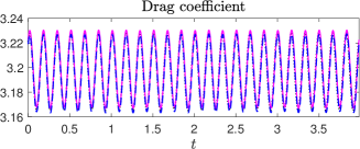
Refer to caption    Refer to caption

Figure 5: Drag (left) and lift (right) coefficients for the reference solution (black, dotted line), the FOM (magenta, continuous line), and the POD-ROM approximation with snapshots 𝒖hjsuperscriptsubscript𝒖𝑗\boldsymbol{u}_{h}^{j} as data set and L2superscript𝐿2L^{2} inner product (blue, discontinuous line).

At first sight, the agreement is excellent. Fig. 6 compares the first and twelfth periods. There is a phase difference between the black dotted line and the other two lines, since, as commented above, the “exact” solution computed on the refined grid has a slightly different period than that computed on the main grid. We notice however, that the difference between the other two lines is hardly altered from the first period to the last one.
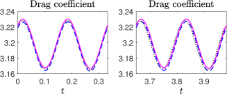
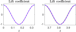
Refer to caption    Refer to caption

Figure 6: Drag (left) and lift (right) coefficients for the reference solution (black, dotted line), the FOM (magenta, continuous line), and the POD-ROM approximation with snapshots 𝒖hjsuperscriptsubscript𝒖𝑗\boldsymbol{u}_{h}^{j} as data set and L2superscript𝐿2L^{2} inner product (blue, discontinuous line).

In addition, the results for the lift coefficient corresponding to the FOM and the POD-ROM approximation are on top of each other (in fact the maximum relative error of this coefficient with respect to that of the FOM in the 12 periods is below 1.7×1041.7superscript1041.7\times 10^{-4}). Some differences can be seen in the drag coefficient. However, the maximum relative error with respect the coefficient computed with the FOM is below 0.0011.

The summary of the results is that there are no significant differences in the POD-ROM approximation, i.e., they are quite independent of the data set used. Only some minor differences, namely that the projection errors depend on the data set when the H01superscriptsubscript𝐻01H_{0}^{1} inner product is used, could be observed in the computation of the POD basis.

6 Conclusions

We analyzed reduced order models for the incompressible Navier–Stokes equations based on proper orthogonal decomposition methods. The influence of including approximations to the time derivative in the set of snapshots was studied. Our set of snapshots is constituted by the approximation to the velocity at the initial time together with approximations to the time derivative at different times. The approximation to the velocity at the initial time can be replaced by the mean value and then only approximations to the time derivatives are required for applying the POD method to the fluctuations. The Galerkin time derivative can be replaced by any other approximation as the standard difference quotient.

We studied the differences between projecting onto L2superscript𝐿2L^{2} and H01superscriptsubscript𝐻01{H_{0}^{1}}. We proved that including the Galerkin time derivatives (or the difference quotients) leads to pointwise estimates for both projections. In the L2superscript𝐿2L^{2} case, error bounds can be proved in the no-time-derivatives case (with only snapshots for the velocity) as shown in the literature, e.g., see [26]. However, the time derivatives approach is useful also in this case to get pointwise estimates. In the numerical analysis, we utilized the projection of the continuous-in-time Galerkin approximation since this allows to use in practice any time integrator for computing the snapshots. It is easy to include the corresponding error in time in the bounds of the present paper. Also, different times can be considered to compute the set of snapshots and the fully discrete POD approximations. Finally, as in one of the methods in [26], we added grad-div stabilization to the approximations computed with the FOM and POD methods to be able to prove error bounds in which the constants do not depend on inverse powers of the viscosity.

In the numerical studies, we compared three different sets of snapshots, for both inner products, where the elements in the data sets were 𝒚hj=𝒖hj𝒖¯hsuperscriptsubscript𝒚𝑗superscriptsubscript𝒖𝑗subscript¯𝒖\boldsymbol{y}_{h}^{j}=\boldsymbol{u}_{h}^{j}-\overline{\boldsymbol{u}}_{h}, 𝒚hj=T𝒖u,tjsuperscriptsubscript𝒚𝑗𝑇superscriptsubscript𝒖𝑢𝑡𝑗\boldsymbol{y}_{h}^{j}=T\boldsymbol{u}_{u,t}^{j}, and 𝒚hj=Tδt𝒖hj=T(𝒖hj𝒖hj1)/Δtsuperscriptsubscript𝒚𝑗𝑇subscript𝛿𝑡superscriptsubscript𝒖𝑗𝑇superscriptsubscript𝒖𝑗superscriptsubscript𝒖𝑗1Δ𝑡\boldsymbol{y}_{h}^{j}=T\delta_{t}\boldsymbol{u}_{h}^{j}=T(\boldsymbol{u}_{h}^{j}-\boldsymbol{u}_{h}^{j-1})/\Delta t. While the snapshots were computed using only one period, we showed that very good approximations are obtained to the lift and drag coefficients in a time interval of 12 periods. In our numerical studies there were no significant differences between the different procedures. More comprehensive studies have to further investigate this topic.

Altogether, we think that the rigorous numerical analysis presented in this paper shows interesting properties and sharp bounds for the different methods. It also supports the idea of the recent paper [25] which shows that in the case of the heat equation there is no need to include in the set of snapshots other than one approximation to the solution at a fixed time. We prove that for the approximation to the incompressible Navier–Stokes equations the same situation holds. Moreover, in case of applying the POD method to fluctuations, as it is standard, only snapshots of the time derivative are needed.

Appendix A Robust bounds for the terms with the second temporal derivative

In this section we derive bounds for the terms (72) and (68). As a consequence, the terms on the right-hand sides of (4.1) and (71) that contain (68) and (72), respectively, are bounded.

The constants in the bounds below do not blow up as ν0𝜈0\nu\to 0. It will be assumed that all functions are sufficiently smooth such that the performed operations are well defined.

Lemma A.1.

Let 𝐮hsubscript𝐮\boldsymbol{u}_{h} be the Galerkin approximation defined in (14) and let 𝐬hmsuperscriptsubscript𝐬𝑚\boldsymbol{s}_{h}^{m} be the modified Stokes projection defined in (7). Let us denote by 𝐞h=𝐮h𝐬hmsubscript𝐞subscript𝐮superscriptsubscript𝐬𝑚\boldsymbol{e}_{h}=\boldsymbol{u}_{h}-\boldsymbol{s}_{h}^{m}. Assume for simplicity 𝐮h(0)=𝐬hm(0)subscript𝐮0superscriptsubscript𝐬𝑚0\boldsymbol{u}_{h}(0)=\boldsymbol{s}_{h}^{m}(0). Then, the following bounds hold

(76) 0t𝒆h,t(s)02𝑑ssuperscriptsubscript0𝑡superscriptsubscriptnormsubscript𝒆𝑡𝑠02differential-d𝑠\displaystyle\int_{0}^{t}\|\boldsymbol{e}_{h,t}(s)\|_{0}^{2}\ ds \displaystyle\leq Ch2(l1),𝐶superscript2𝑙1\displaystyle Ch^{2(l-1)},
(77) 0t𝒆h,tt(s)02𝑑ssuperscriptsubscript0𝑡superscriptsubscriptnormsubscript𝒆𝑡𝑡𝑠02differential-d𝑠\displaystyle\int_{0}^{t}\|\boldsymbol{e}_{h,tt}(s)\|_{0}^{2}\ ds \displaystyle\leq Ch2(l2),𝐶superscript2𝑙2\displaystyle Ch^{2(l-2)},
(78) 0t(𝒆h,tt)(s)02𝑑ssuperscriptsubscript0𝑡superscriptsubscriptnormsubscript𝒆𝑡𝑡𝑠02differential-d𝑠\displaystyle\int_{0}^{t}\|\nabla(\boldsymbol{e}_{h,tt})(s)\|_{0}^{2}\ ds \displaystyle\leq Ch2(l3),𝐶superscript2𝑙3\displaystyle Ch^{2(l-3)},

where the constant C𝐶C is independent of inverse powers of ν𝜈\nu.

Proof A.2.

We bound

(79) 𝒖h,tt0𝒖h,tt𝒔h,ttm0+𝒖tt0+𝒔h,ttm𝒖tt0,subscriptnormsubscript𝒖𝑡𝑡0subscriptnormsubscript𝒖𝑡𝑡subscriptsuperscript𝒔𝑚𝑡𝑡0subscriptnormsubscript𝒖𝑡𝑡0subscriptnormsubscriptsuperscript𝒔𝑚𝑡𝑡subscript𝒖𝑡𝑡0\|\boldsymbol{u}_{h,tt}\|_{0}\leq\|\boldsymbol{u}_{h,tt}-\boldsymbol{s}^{m}_{h,tt}\|_{0}+\|\boldsymbol{u}_{tt}\|_{0}+\|\boldsymbol{s}^{m}_{h,tt}-\boldsymbol{u}_{tt}\|_{0},

and likewise for the norm of the gradient. Below, the first term on the right-hand side will be shown to be bounded. The second term is bounded because the solution is sufficiently smooth, and then the last term can be bounded with (8), where the notation 𝐬h,ttmsubscriptsuperscript𝐬𝑚𝑡𝑡\boldsymbol{s}^{m}_{h,tt} has to be understood that the modified Stokes projection is applied to 𝐮ttsubscript𝐮𝑡𝑡\boldsymbol{u}_{tt}.

The error equation for (14) is given by

(80) (𝒆h,t,𝝋h)+ν(𝒆h,𝝋h)+bh(𝒖h,𝒖h,𝝋h)bh(𝒖,𝒖,𝝋h)+μ(𝒆h,𝝋h)subscript𝒆𝑡subscript𝝋𝜈subscript𝒆subscript𝝋subscript𝑏subscript𝒖subscript𝒖subscript𝝋subscript𝑏𝒖𝒖subscript𝝋𝜇subscript𝒆subscript𝝋\displaystyle\left(\boldsymbol{e}_{h,t},\boldsymbol{\varphi}_{h}\right)+\nu(\nabla\boldsymbol{e}_{h},\nabla\boldsymbol{\varphi}_{h})+b_{h}(\boldsymbol{u}_{h},\boldsymbol{u}_{h},\boldsymbol{\varphi}_{h})-b_{h}(\boldsymbol{u},\boldsymbol{u},\boldsymbol{\varphi}_{h})+\mu(\nabla\cdot\boldsymbol{e}_{h},\nabla\cdot\boldsymbol{\varphi}_{h})
=\displaystyle= (σ1,𝝋h)+(σ2,𝝋h)𝝋h𝑽hl,subscript𝜎1subscript𝝋subscript𝜎2subscript𝝋for-allsubscript𝝋superscriptsubscript𝑽𝑙\displaystyle(\sigma_{1},\boldsymbol{\varphi}_{h})+(\sigma_{2},\nabla\cdot\boldsymbol{\varphi}_{h})\quad\forall\ \boldsymbol{\varphi}_{h}\in{\boldsymbol{V}}_{h}^{l},

with σ1=𝐮t𝐬h,tmsubscript𝜎1subscript𝐮𝑡subscriptsuperscript𝐬𝑚𝑡\sigma_{1}=\boldsymbol{u}_{t}-\boldsymbol{s}^{m}_{h,t}, σ2=(pPQhp)+μ((𝐮𝐬hm)\sigma_{2}=(p-P_{Q_{h}}p)+\mu(\nabla\cdot(\boldsymbol{u}-\boldsymbol{s}_{h}^{m}), and PQhpsubscript𝑃subscript𝑄𝑝P_{Q_{h}}p is the best approximation of p𝑝p in Qhlsuperscriptsubscript𝑄𝑙Q_{h}^{l}. Note that if a (discrete) velocity function is in 𝐕𝐕\boldsymbol{V} (or 𝐕hlsuperscriptsubscript𝐕𝑙{\boldsymbol{V}}_{h}^{l}), then also the temporal derivatives of this function are in the same space. Hence, taking 𝛗h=𝐞h,t𝐕hlsubscript𝛗subscript𝐞𝑡superscriptsubscript𝐕𝑙\boldsymbol{\varphi}_{h}=\boldsymbol{e}_{h,t}\in{\boldsymbol{V}}_{h}^{l} in (80) and using the inverse inequality (6) yields

(81) 𝒆h,t02+ddt12ν𝒆h02+ddt12μ𝒆h02|bh(𝒖h𝒖,𝒖,𝒆h,t)|superscriptsubscriptnormsubscript𝒆𝑡02𝑑𝑑𝑡12𝜈superscriptsubscriptnormsubscript𝒆02𝑑𝑑𝑡12𝜇superscriptsubscriptnormsubscript𝒆02subscript𝑏subscript𝒖𝒖𝒖subscript𝒆𝑡\displaystyle\|\boldsymbol{e}_{h,t}\|_{0}^{2}+\frac{d}{dt}\frac{1}{2}\nu\|\nabla\boldsymbol{e}_{h}\|_{0}^{2}+\frac{d}{dt}\frac{1}{2}\mu\|\nabla\cdot\boldsymbol{e}_{h}\|_{0}^{2}\leq|b_{h}(\boldsymbol{u}_{h}-\boldsymbol{u},\boldsymbol{u},\boldsymbol{e}_{h,t})|
+|bh(𝒖h,𝒖h𝒖,𝒆h,t)|+σ10𝒆h,t0+cinvσ20h1𝒆h,t0.subscript𝑏subscript𝒖subscript𝒖𝒖subscript𝒆𝑡subscriptnormsubscript𝜎10subscriptnormsubscript𝒆𝑡0subscript𝑐invsubscriptnormsubscript𝜎20superscript1subscriptnormsubscript𝒆𝑡0\displaystyle+|b_{h}(\boldsymbol{u}_{h},\boldsymbol{u}_{h}-\boldsymbol{u},\boldsymbol{e}_{h,t})|+\|\sigma_{1}\|_{0}\|\boldsymbol{e}_{h,t}\|_{0}+c_{\rm inv}\|\sigma_{2}\|_{0}h^{-1}\|\boldsymbol{e}_{h,t}\|_{0}.

The first term on the right-hand side is estimated with Hölder’s inequality, (15), and Young’s inequality

|bh(𝒖h𝒖,𝒖,𝒆h,t)|subscript𝑏subscript𝒖𝒖𝒖subscript𝒆𝑡\displaystyle|b_{h}(\boldsymbol{u}_{h}-\boldsymbol{u},\boldsymbol{u},\boldsymbol{e}_{h,t})| \displaystyle\leq 𝒖h𝒖0𝒖𝒆h,t0+12(𝒖h𝒖)0𝒖𝒆h,t0subscriptnormsubscript𝒖𝒖0subscriptnorm𝒖subscriptnormsubscript𝒆𝑡012subscriptnormsubscript𝒖𝒖0subscriptnorm𝒖subscriptnormsubscript𝒆𝑡0\displaystyle\|\boldsymbol{u}_{h}-\boldsymbol{u}\|_{0}\|\nabla\boldsymbol{u}\|_{\infty}\|\boldsymbol{e}_{h,t}\|_{0}+\frac{1}{2}\|\nabla\cdot(\boldsymbol{u}_{h}-\boldsymbol{u})\|_{0}\|\boldsymbol{u}\|_{\infty}\|\boldsymbol{e}_{h,t}\|_{0}
\displaystyle\leq Ch2(l1)+18𝒆h,t02.𝐶superscript2𝑙118superscriptsubscriptnormsubscript𝒆𝑡02\displaystyle Ch^{2(l-1)}+\frac{1}{8}\|\boldsymbol{e}_{h,t}\|_{0}^{2}.

For the second term, in addition the following estimate from [18, Lemma 6.11]

((𝒖)𝒗,𝒘)C𝒖1𝒗0𝒘1,𝒖,𝒗,𝒘H1(Ω)d,formulae-sequence𝒖𝒗𝒘𝐶subscriptnorm𝒖1subscriptnorm𝒗0subscriptnorm𝒘1𝒖𝒗𝒘superscript𝐻1superscriptΩ𝑑((\boldsymbol{u}\cdot\nabla)\boldsymbol{v},\boldsymbol{w})\leq C\|\boldsymbol{u}\|_{1}\|\nabla\boldsymbol{v}\|_{0}\|\boldsymbol{w}\|_{1},\quad\boldsymbol{u},\boldsymbol{v},\boldsymbol{w}\in H^{1}(\Omega)^{d},

the inverse inequality (6), and the condition l2𝑙2l\geq 2 are utilized

|bh(𝒖h,𝒖h𝒖,𝒆h,t)|subscript𝑏subscript𝒖subscript𝒖𝒖subscript𝒆𝑡\displaystyle|b_{h}(\boldsymbol{u}_{h},\boldsymbol{u}_{h}-\boldsymbol{u},\boldsymbol{e}_{h,t})| \displaystyle\leq |bh(𝒖h𝒖,𝒖h𝒖,𝒆h,t)|+|bh(𝒖,𝒖h𝒖,𝒆h,t)|subscript𝑏subscript𝒖𝒖subscript𝒖𝒖subscript𝒆𝑡subscript𝑏𝒖subscript𝒖𝒖subscript𝒆𝑡\displaystyle|b_{h}(\boldsymbol{u}_{h}-\boldsymbol{u},\boldsymbol{u}_{h}-\boldsymbol{u},\boldsymbol{e}_{h,t})|+|b_{h}(\boldsymbol{u},\boldsymbol{u}_{h}-\boldsymbol{u},\boldsymbol{e}_{h,t})|
\displaystyle\leq C𝒖h𝒖12𝒆h,t1+𝒖(𝒖h𝒖)0𝒆h,t0𝐶superscriptsubscriptnormsubscript𝒖𝒖12subscriptnormsubscript𝒆𝑡1subscriptnorm𝒖subscriptnormsubscript𝒖𝒖0subscriptnormsubscript𝒆𝑡0\displaystyle C\|\boldsymbol{u}_{h}-\boldsymbol{u}\|_{1}^{2}\|\boldsymbol{e}_{h,t}\|_{1}+\|\boldsymbol{u}\|_{\infty}\|\nabla(\boldsymbol{u}_{h}-\boldsymbol{u})\|_{0}\|\boldsymbol{e}_{h,t}\|_{0}
\displaystyle\leq C𝒖h𝒖12cinvh1𝒆h,t0+C𝒖h𝒖1𝒆h,t0𝐶superscriptsubscriptnormsubscript𝒖𝒖12subscript𝑐invsuperscript1subscriptnormsubscript𝒆𝑡0𝐶subscriptnormsubscript𝒖𝒖1subscriptnormsubscript𝒆𝑡0\displaystyle C\|\boldsymbol{u}_{h}-\boldsymbol{u}\|_{1}^{2}c_{\rm inv}h^{-1}\|\boldsymbol{e}_{h,t}\|_{0}+C\|\boldsymbol{u}_{h}-\boldsymbol{u}\|_{1}\|\boldsymbol{e}_{h,t}\|_{0}
\displaystyle\leq C(h4l6+h2l2)+18𝒆h,t02Ch2(l1)+18𝒆h,t02.𝐶superscript4𝑙6superscript2𝑙218superscriptsubscriptnormsubscript𝒆𝑡02𝐶superscript2𝑙118superscriptsubscriptnormsubscript𝒆𝑡02\displaystyle C\left(h^{4l-6}+h^{2l-2}\right)+\frac{1}{8}\|\boldsymbol{e}_{h,t}\|_{0}^{2}\leq Ch^{2(l-1)}+\frac{1}{8}\|\boldsymbol{e}_{h,t}\|_{0}^{2}.

For the last two terms, we obtain, with (8), the L2(Ω)superscript𝐿2ΩL^{2}(\Omega) best approximation error for the pressure, and Young’s inequality, the following bound

σ10𝒆h,t0+cinvσ20h1𝒆h,t0subscriptnormsubscript𝜎10subscriptnormsubscript𝒆𝑡0subscript𝑐invsubscriptnormsubscript𝜎20superscript1subscriptnormsubscript𝒆𝑡0\displaystyle\|\sigma_{1}\|_{0}\|\boldsymbol{e}_{h,t}\|_{0}+c_{\rm inv}\|\sigma_{2}\|_{0}h^{-1}\|\boldsymbol{e}_{h,t}\|_{0} \displaystyle\leq 2σ102+cinv2σ202h2+14𝒆h,t022superscriptsubscriptnormsubscript𝜎102superscriptsubscript𝑐inv2superscriptsubscriptnormsubscript𝜎202superscript214superscriptsubscriptnormsubscript𝒆𝑡02\displaystyle 2\|\sigma_{1}\|_{0}^{2}+c_{\rm inv}^{2}\|\sigma_{2}\|_{0}^{2}h^{-2}+\frac{1}{4}\|\boldsymbol{e}_{h,t}\|_{0}^{2}
\displaystyle\leq Ch2(l1)+14𝒆h,t02.𝐶superscript2𝑙114superscriptsubscriptnormsubscript𝒆𝑡02\displaystyle Ch^{2(l-1)}+\frac{1}{4}\|\boldsymbol{e}_{h,t}\|_{0}^{2}.

Absorbing terms in the left-hand side of (81) and collecting the other terms on the right-hand side leads to

(82) 12(𝒆h,t02+ddtν𝒆h02+ddtμ𝒆h02)Ch2(l1),12superscriptsubscriptnormsubscript𝒆𝑡02𝑑𝑑𝑡𝜈superscriptsubscriptnormsubscript𝒆02𝑑𝑑𝑡𝜇superscriptsubscriptnormsubscript𝒆02𝐶superscript2𝑙1\frac{1}{2}\left(\|\boldsymbol{e}_{h,t}\|_{0}^{2}+\frac{d}{dt}\nu\|\nabla\boldsymbol{e}_{h}\|_{0}^{2}+\frac{d}{dt}\mu\|\nabla\cdot\boldsymbol{e}_{h}\|_{0}^{2}\right)\leq Ch^{2(l-1)},

from which, taking into account 𝐞h(0)=0subscript𝐞00\boldsymbol{e}_{h}(0)=0, we derive the estimate

0t𝒆h,t(s)02𝑑s+ν𝒆h(t)02+μ𝒆h(t)02Ch2(l1).superscriptsubscript0𝑡superscriptsubscriptnormsubscript𝒆𝑡𝑠02differential-d𝑠𝜈superscriptsubscriptnormsubscript𝒆𝑡02𝜇superscriptsubscriptnormsubscript𝒆𝑡02𝐶superscript2𝑙1\int_{0}^{t}\|\boldsymbol{e}_{h,t}(s)\|_{0}^{2}\ ds+\nu\|\nabla\boldsymbol{e}_{h}(t)\|_{0}^{2}+\mu\|\nabla\cdot\boldsymbol{e}_{h}(t)\|_{0}^{2}\leq Ch^{2(l-1)}.

so that (76) holds.

Considering t0𝑡0t\to 0 in (80), the viscous term and the grad-div stabilization term vanish, since 𝐞h(0)=𝟎subscript𝐞00\boldsymbol{e}_{h}(0)=\boldsymbol{0}. Following [15] the initial pressure p(0)𝑝0p(0) is the solution of the problem

Δp(0)Δ𝑝0\displaystyle\Delta p(0) =\displaystyle= 𝒇(0)((𝒖0)𝒖0)in Ω,𝒇0superscript𝒖0superscript𝒖0in Ω\displaystyle\nabla\cdot\boldsymbol{f}(0)-\nabla\cdot((\boldsymbol{u}^{0}\cdot\nabla)\boldsymbol{u}^{0})\quad\mbox{in }\Omega,
p(0)𝒏𝑝0𝒏\displaystyle\frac{\partial p(0)}{\partial\boldsymbol{n}} =\displaystyle= (νΔ𝒖0+𝒇(0)(𝒖0)𝒖0)𝒏on Ω,𝜈Δsuperscript𝒖0𝒇0superscript𝒖0superscript𝒖0𝒏on Ω\displaystyle(\nu\Delta\boldsymbol{u}^{0}+\boldsymbol{f}(0)-(\boldsymbol{u}^{0}\cdot\nabla)\boldsymbol{u}^{0})\cdot\boldsymbol{n}\quad\mbox{on }\partial\Omega,

where 𝐧𝐧\boldsymbol{n} is the outward pointing unit normal vector The above problem defines a unique pressure up to a constant. Then, one can repeat the same analysis as above at time t=0𝑡0t=0 starting from (81) (with only the term 𝐞h,t(0)02superscriptsubscriptnormsubscript𝐞𝑡002\|\boldsymbol{e}_{h,t}(0)\|_{0}^{2} on the left-hand side) and obtains, instead of (82),

12𝒆h,t(0)02Ch2(l1).12superscriptsubscriptnormsubscript𝒆𝑡002𝐶superscript2𝑙1\frac{1}{2}\|\boldsymbol{e}_{h,t}(0)\|_{0}^{2}\leq Ch^{2(l-1)}.

Applying the inverse inequality yields

(83) (𝒆h,t)(0)02Ch2(l2),(𝒆h,t)(0)02Ch2(l2),formulae-sequencesuperscriptsubscriptnormsubscript𝒆𝑡002𝐶superscript2𝑙2superscriptsubscriptnormsubscript𝒆𝑡002𝐶superscript2𝑙2\|(\nabla\boldsymbol{e}_{h,t})(0)\|_{0}^{2}\leq Ch^{2(l-2)},\quad\|(\nabla\cdot\boldsymbol{e}_{h,t})(0)\|_{0}^{2}\leq Ch^{2(l-2)},

such that the norms on the left-hand sides are bounded for l2𝑙2l\geq 2.

Taking the time derivative of (80) gives

(𝒆h,tt,𝝋h)+ν(𝒆h,t,𝝋h)+bh(𝒖h,t,𝒖h,𝝋h)bh(𝒖t,𝒖,𝝋h)subscript𝒆𝑡𝑡subscript𝝋𝜈subscript𝒆𝑡subscript𝝋subscript𝑏subscript𝒖𝑡subscript𝒖subscript𝝋subscript𝑏subscript𝒖𝑡𝒖subscript𝝋\displaystyle\left(\boldsymbol{e}_{h,tt},\boldsymbol{\varphi}_{h}\right)+\nu(\nabla\boldsymbol{e}_{h,t},\nabla\boldsymbol{\varphi}_{h})+b_{h}(\boldsymbol{u}_{h,t},\boldsymbol{u}_{h},\boldsymbol{\varphi}_{h})-b_{h}(\boldsymbol{u}_{t},\boldsymbol{u},\boldsymbol{\varphi}_{h})
+bh(𝒖h,𝒖h,t,𝝋h)bh(𝒖,𝒖t,𝝋h)+μ(𝒆h,t,𝝋h)subscript𝑏subscript𝒖subscript𝒖𝑡subscript𝝋subscript𝑏𝒖subscript𝒖𝑡subscript𝝋𝜇subscript𝒆𝑡subscript𝝋\displaystyle+b_{h}(\boldsymbol{u}_{h},\boldsymbol{u}_{h,t},\boldsymbol{\varphi}_{h})-b_{h}(\boldsymbol{u},\boldsymbol{u}_{t},\boldsymbol{\varphi}_{h})+\mu(\nabla\cdot\boldsymbol{e}_{h,t},\nabla\cdot\boldsymbol{\varphi}_{h})
=\displaystyle= (σ1,t,𝝋h)+(σ2,t,𝝋h)𝝋h𝑽hl,subscript𝜎1𝑡subscript𝝋subscript𝜎2𝑡subscript𝝋for-allsubscript𝝋superscriptsubscript𝑽𝑙\displaystyle(\sigma_{1,t},\boldsymbol{\varphi}_{h})+(\sigma_{2,t},\nabla\cdot\boldsymbol{\varphi}_{h})\quad\forall\ \boldsymbol{\varphi}_{h}\in{\boldsymbol{V}}_{h}^{l},

Choosing 𝛗h=𝐞h,ttsubscript𝛗subscript𝐞𝑡𝑡\boldsymbol{\varphi}_{h}=\boldsymbol{e}_{h,tt} and arguing as before leads to

(85) 𝒆h,tt02+ddt12ν𝒆h,t02+ddt12μ𝒆h,t02superscriptsubscriptnormsubscript𝒆𝑡𝑡02𝑑𝑑𝑡12𝜈superscriptsubscriptnormsubscript𝒆𝑡02𝑑𝑑𝑡12𝜇superscriptsubscriptnormsubscript𝒆𝑡02\displaystyle\|\boldsymbol{e}_{h,tt}\|_{0}^{2}+\frac{d}{dt}\frac{1}{2}\nu\|\nabla\boldsymbol{e}_{h,t}\|_{0}^{2}+\frac{d}{dt}\frac{1}{2}\mu\|\nabla\cdot\boldsymbol{e}_{h,t}\|_{0}^{2}
\displaystyle\leq σ1,t02+cinv2h2σ2,t02+14𝒆h,tt02+|bh(𝒖h,t𝒖t,𝒖,𝒆h,tt)|superscriptsubscriptnormsubscript𝜎1𝑡02superscriptsubscript𝑐inv2superscript2superscriptsubscriptnormsubscript𝜎2𝑡0214superscriptsubscriptnormsubscript𝒆𝑡𝑡02subscript𝑏subscript𝒖𝑡subscript𝒖𝑡𝒖subscript𝒆𝑡𝑡\displaystyle\|\sigma_{1,t}\|_{0}^{2}+c_{\rm inv}^{2}h^{-2}\|\sigma_{2,t}\|_{0}^{2}+\frac{1}{4}\|\boldsymbol{e}_{h,tt}\|_{0}^{2}+|b_{h}(\boldsymbol{u}_{h,t}-\boldsymbol{u}_{t},\boldsymbol{u},\boldsymbol{e}_{h,tt})|
+|bh(𝒖h,t,𝒖𝒖h,𝒆h,tt)|+|bh(𝒖h𝒖,𝒖t,𝒆h,tt)|+|bh(𝒖h,𝒖t𝒖h,t,𝒆h,tt)|.subscript𝑏subscript𝒖𝑡𝒖subscript𝒖subscript𝒆𝑡𝑡subscript𝑏subscript𝒖𝒖subscript𝒖𝑡subscript𝒆𝑡𝑡subscript𝑏subscript𝒖subscript𝒖𝑡subscript𝒖𝑡subscript𝒆𝑡𝑡\displaystyle+|b_{h}(\boldsymbol{u}_{h,t},\boldsymbol{u}-\boldsymbol{u}_{h},\boldsymbol{e}_{h,tt})|+|b_{h}(\boldsymbol{u}_{h}-\boldsymbol{u},\boldsymbol{u}_{t},\boldsymbol{e}_{h,tt})|+|b_{h}(\boldsymbol{u}_{h},\boldsymbol{u}_{t}-\boldsymbol{u}_{h,t},\boldsymbol{e}_{h,tt})|.

Let us observe that the bounds for σ1,t0subscriptnormsubscript𝜎1𝑡0\|\sigma_{1,t}\|_{0} and σ2,t0subscriptnormsubscript𝜎2𝑡0\|\sigma_{2,t}\|_{0} depend on the regularity of 𝐮tsubscript𝐮𝑡\boldsymbol{u}_{t}, 𝐮ttsubscript𝐮𝑡𝑡\boldsymbol{u}_{tt}, and ptsubscript𝑝𝑡p_{t}, but all are bounded if the solution is sufficiently regular. For the nonlinear terms, the same arguments as above are used. For the first term, we obtain

(86) |bh(𝒖h,t𝒖t,𝒖,𝒆h,tt)|subscript𝑏subscript𝒖𝑡subscript𝒖𝑡𝒖subscript𝒆𝑡𝑡\displaystyle|b_{h}(\boldsymbol{u}_{h,t}-\boldsymbol{u}_{t},\boldsymbol{u},\boldsymbol{e}_{h,tt})|
\displaystyle\leq 𝒖h,t𝒖t0𝒖𝒆h,tt0+12(𝒖h,t𝒖t)0𝒖𝒆h,tt0subscriptnormsubscript𝒖𝑡subscript𝒖𝑡0subscriptnorm𝒖subscriptnormsubscript𝒆𝑡𝑡012subscriptnormsubscript𝒖𝑡subscript𝒖𝑡0subscriptnorm𝒖subscriptnormsubscript𝒆𝑡𝑡0\displaystyle\|\boldsymbol{u}_{h,t}-\boldsymbol{u}_{t}\|_{0}\|\nabla\boldsymbol{u}\|_{\infty}\|\boldsymbol{e}_{h,tt}\|_{0}+\frac{1}{2}\|\nabla\cdot(\boldsymbol{u}_{h,t}-\boldsymbol{u}_{t})\|_{0}\|\boldsymbol{u}\|_{\infty}\|\boldsymbol{e}_{h,tt}\|_{0}
\displaystyle\leq C𝒖t𝒖h,t12+116𝒆h,tt02.𝐶superscriptsubscriptnormsubscript𝒖𝑡subscript𝒖𝑡12116superscriptsubscriptnormsubscript𝒆𝑡𝑡02\displaystyle C\|\boldsymbol{u}_{t}-\boldsymbol{u}_{h,t}\|_{1}^{2}+\frac{1}{16}\|\boldsymbol{e}_{h,tt}\|_{0}^{2}.

It follows from (8), (76), and the inverse inequality (6) that

0t𝒖t𝒖h,t12Ch2(l2),superscriptsubscript0𝑡superscriptsubscriptnormsubscript𝒖𝑡subscript𝒖𝑡12𝐶superscript2𝑙2\int_{0}^{t}\|\boldsymbol{u}_{t}-\boldsymbol{u}_{h,t}\|_{1}^{2}\leq Ch^{2(l-2)},

so that absorbing the second term on the right-hand side of (86) in the left-hand side of (85) and integrating in time, the corresponding first term on the right-hand side of (86) is bounded. For the second nonlinear term on the right-hand side of (85), we obtain

|bh(𝒖h,t,𝒖𝒖h,𝒆h,tt)|subscript𝑏subscript𝒖𝑡𝒖subscript𝒖subscript𝒆𝑡𝑡\displaystyle|b_{h}(\boldsymbol{u}_{h,t},\boldsymbol{u}-\boldsymbol{u}_{h},\boldsymbol{e}_{h,tt})| \displaystyle\leq C𝒖h,t1𝒖𝒖h1cinvh1𝒆h,tt0𝐶subscriptnormsubscript𝒖𝑡1subscriptnorm𝒖subscript𝒖1subscript𝑐invsuperscript1subscriptnormsubscript𝒆𝑡𝑡0\displaystyle C\|\boldsymbol{u}_{h,t}\|_{1}\|\boldsymbol{u}-\boldsymbol{u}_{h}\|_{1}c_{\rm inv}h^{-1}\|\boldsymbol{e}_{h,tt}\|_{0}
\displaystyle\leq Ch2(l2)𝒖h,t12+116𝒆h,tt02.𝐶superscript2𝑙2superscriptsubscriptnormsubscript𝒖𝑡12116superscriptsubscriptnormsubscript𝒆𝑡𝑡02\displaystyle Ch^{2(l-2)}\|\boldsymbol{u}_{h,t}\|_{1}^{2}+\frac{1}{16}\|\boldsymbol{e}_{h,tt}\|_{0}^{2}.

Again, the last term on the right-hand side can be absorbed in the left-hand side of (85) and the integral with respect to time of the first term is bounded. For the third nonlinear term we argue as for the second one to get

|bh(𝒖h𝒖,𝒖t,𝒆h,tt)|𝒖h𝒖1𝒖t1𝒆h,tt1Ch2(l2)𝒖t12+116𝒆h,tt02.subscript𝑏subscript𝒖𝒖subscript𝒖𝑡subscript𝒆𝑡𝑡subscriptnormsubscript𝒖𝒖1subscriptnormsubscript𝒖𝑡1subscriptnormsubscript𝒆𝑡𝑡1𝐶superscript2𝑙2superscriptsubscriptnormsubscript𝒖𝑡12116superscriptsubscriptnormsubscript𝒆𝑡𝑡02|b_{h}(\boldsymbol{u}_{h}-\boldsymbol{u},\boldsymbol{u}_{t},\boldsymbol{e}_{h,tt})|\leq\|\boldsymbol{u}_{h}-\boldsymbol{u}\|_{1}\|\boldsymbol{u}_{t}\|_{1}\|\boldsymbol{e}_{h,tt}\|_{1}\leq Ch^{2(l-2)}\|\boldsymbol{u}_{t}\|_{1}^{2}+\frac{1}{16}\|\boldsymbol{e}_{h,tt}\|_{0}^{2}.

Using for the fourth nonlinear term the inverse inequality (6) and (8) gives

|bh(𝒖h,𝒖t𝒖h,t,𝒆h,tt)|𝒖h𝒖t𝒖h,t1𝒆h,tt0subscript𝑏subscript𝒖subscript𝒖𝑡subscript𝒖𝑡subscript𝒆𝑡𝑡subscriptnormsubscript𝒖subscriptnormsubscript𝒖𝑡subscript𝒖𝑡1subscriptnormsubscript𝒆𝑡𝑡0\displaystyle|b_{h}(\boldsymbol{u}_{h},\boldsymbol{u}_{t}-\boldsymbol{u}_{h,t},\boldsymbol{e}_{h,tt})|\leq\|\boldsymbol{u}_{h}\|_{\infty}\|\boldsymbol{u}_{t}-\boldsymbol{u}_{h,t}\|_{1}\|\boldsymbol{e}_{h,tt}\|_{0}
+12(𝒖h𝒔h)𝒖t𝒖h,t0𝒆h,tt0+12𝒔h𝒖t𝒖h,t0𝒆h,tt012subscriptnormsubscript𝒖subscript𝒔subscriptnormsubscript𝒖𝑡subscript𝒖𝑡0subscriptnormsubscript𝒆𝑡𝑡012subscriptnormsubscript𝒔subscriptnormsubscript𝒖𝑡subscript𝒖𝑡0subscriptnormsubscript𝒆𝑡𝑡0\displaystyle+\frac{1}{2}\|\nabla\cdot(\boldsymbol{u}_{h}-\boldsymbol{s}_{h})\|_{\infty}\|\boldsymbol{u}_{t}-\boldsymbol{u}_{h,t}\|_{0}\|\boldsymbol{e}_{h,tt}\|_{0}+\frac{1}{2}\|\nabla\cdot\boldsymbol{s}_{h}\|_{\infty}\|\boldsymbol{u}_{t}-\boldsymbol{u}_{h,t}\|_{0}\|\boldsymbol{e}_{h,tt}\|_{0}
\displaystyle\leq C(𝒖t𝒖h,t12+cinv2hdh2(l1)𝒖t𝒖h,t02)+116𝒆h,tt02.𝐶superscriptsubscriptnormsubscript𝒖𝑡subscript𝒖𝑡12superscriptsubscript𝑐inv2superscript𝑑superscript2𝑙1superscriptsubscriptnormsubscript𝒖𝑡subscript𝒖𝑡02116superscriptsubscriptnormsubscript𝒆𝑡𝑡02\displaystyle C\left(\|\boldsymbol{u}_{t}-\boldsymbol{u}_{h,t}\|_{1}^{2}+c_{\rm inv}^{2}h^{-d}h^{2(l-1)}\|\boldsymbol{u}_{t}-\boldsymbol{u}_{h,t}\|_{0}^{2}\right)+\frac{1}{16}\|\boldsymbol{e}_{h,tt}\|_{0}^{2}.

Again, the last term on the right-hand side above is absorbed into the left-hand side of (85), the integral of the first term is bounded, and the integral for the second is

cinv2hdh2(l1)0t𝒖t𝒖h,t(s)02𝑑sCh4l4d,superscriptsubscript𝑐inv2superscript𝑑superscript2𝑙1superscriptsubscript0𝑡superscriptsubscriptnormsubscript𝒖𝑡subscript𝒖𝑡𝑠02differential-d𝑠𝐶superscript4𝑙4𝑑c_{\rm inv}^{2}h^{-d}h^{2(l-1)}\int_{0}^{t}\|\boldsymbol{u}_{t}-\boldsymbol{u}_{h,t}(s)\|_{0}^{2}\ ds\leq Ch^{4l-4-d},

which is bounded since l2𝑙2l\geq 2. Collecting all error bounds and taking (83) into account, we conclude (77) where the constant does not depend explicitly on inverse powers of ν𝜈\nu. The inverse inequality gives (78).

Estimate (77) can be applied, in combination with (79), in (71). To bound (68), which is the term appearing in (4.1), we apply (78) such that a robust estimate is proved only for pairs of finite element spaces with l3𝑙3l\geq 3.

References

  • [1] R. A. Adams, Sobolev spaces, Academic Press [A subsidiary of Harcourt Brace Jovanovich, Publishers], New York-London, 1975. Pure and Applied Mathematics, Vol. 65.
  • [2] F. Brezzi and R. S. Falk, Stability of higher-order Hood-Taylor methods, SIAM J. Numer. Anal., 28 (1991), pp. 581–590, https://doi.org/10.1137/0728032.
  • [3] A. Caiazzo, T. Iliescu, V. John, and S. Schyschlowa, A numerical investigation of velocity-pressure reduced order models for incompressible flows, J. Comput. Phys., 259 (2014), pp. 598–616, https://doi.org/10.1016/j.jcp.2013.12.004.
  • [4] D. Chapelle, A. Gariah, and J. Sainte-Marie, Galerkin approximation with proper orthogonal decomposition: new error estimates and illustrative examples, ESAIM Math. Model. Numer. Anal., 46 (2012), pp. 731–757, https://doi.org/10.1051/m2an/2011053.
  • [5] H. Chen, Pointwise error estimates for finite element solutions of the Stokes problem, SIAM J. Numer. Anal., 44 (2006), pp. 1–28, https://doi.org/10.1137/S0036142903438100.
  • [6] J.-H. Chen, W. G. Pritchard, and S. J. Tavener, Bifurcation for flow past a cylinder between parallel planes, J. Fluid Mech., 284 (1995), pp. 23–41, https://doi.org/10.1017/S0022112095000255, https://doi.org/10.1017/S0022112095000255.
  • [7] P. G. Ciarlet, The finite element method for elliptic problems, vol. 40 of Classics in Applied Mathematics, Society for Industrial and Applied Mathematics (SIAM), Philadelphia, PA, 2002, https://doi.org/10.1137/1.9780898719208. Reprint of the 1978 original [North-Holland, Amsterdam].
  • [8] J. de Frutos, B. García-Archilla, V. John, and J. Novo, Grad-div stabilization for the evolutionary Oseen problem with inf-sup stable finite elements, J. Sci. Comput., 66 (2016), pp. 991–1024, https://doi.org/10.1007/s10915-015-0052-1.
  • [9] J. de Frutos, B. García-Archilla, V. John, and J. Novo, Analysis of the grad-div stabilization for the time-dependent Navier-Stokes equations with inf-sup stable finite elements, Adv. Comput. Math., 44 (2018), pp. 195–225, https://doi.org/10.1007/s10444-017-9540-1.
  • [10] L. C. Evans, Partial differential equations, vol. 19 of Graduate Studies in Mathematics, American Mathematical Society, Providence, RI, second ed., 2010, https://doi.org/10.1090/gsm/019, https://doi.org/10.1090/gsm/019.
  • [11] B. García-Archilla, V. John, and J. Novo, On the convergence order of the finite element error in the kinetic energy for high Reynolds number incompressible flows, Comput. Methods Appl. Mech. Engrg., 385 (2021), pp. Paper No. 114032, 54, https://doi.org/10.1016/j.cma.2021.114032.
  • [12] B. García-Archilla, J. Novo, and S. Rubino, Error analysis of proper orthogonal decomposition data assimilation schemes with grad-div stabilization for the Navier-Stokes equations, J. Comput. Appl. Math., 411 (2022), pp. Paper No. 114246, 30, https://doi.org/10.1016/j.cam.2022.114246.
  • [13] B. García-Archilla, J. Novo, and E. S. Titi, Uniform in time error estimates for a finite element method applied to a downscaling data assimilation algorithm for the Navier-Stokes equations, SIAM J. Numer. Anal., 58 (2020), pp. 410–429, https://doi.org/10.1137/19M1246845.
  • [14] B. García-Archilla and J. Novo, Robust error bounds for the Navier–Stokes equations using implicit-explicit second-order BDF method with variable steps, IMA Journal of Numerical Analysis, (2022), https://doi.org/10.1093/imanum/drac058.
  • [15] J. G. Heywood and R. Rannacher, Finite element approximation of the nonstationary Navier-Stokes problem. I. Regularity of solutions and second-order error estimates for spatial discretization, SIAM J. Numer. Anal., 19 (1982), pp. 275–311, http://dx.doi.org/10.1137/0719018.
  • [16] J. G. Heywood and R. Rannacher, Finite-element approximation of the nonstationary Navier-Stokes problem. IV. Error analysis for second-order time discretization, SIAM J. Numer. Anal., 27 (1990), pp. 353–384, https://doi.org/10.1137/0727022.
  • [17] T. Iliescu and Z. Wang, Are the snapshot difference quotients needed in the proper orthogonal decomposition?, SIAM J. Sci. Comput., 36 (2014), pp. A1221–A1250, https://doi.org/10.1137/130925141.
  • [18] V. John, Finite element methods for incompressible flow problems, vol. 51 of Springer Series in Computational Mathematics, Springer, Cham, 2016, https://doi.org/10.1007/978-3-319-45750-5.
  • [19] V. John, B. Moreau, and J. Novo, Error analysis of a SUPG-stabilized POD-ROM method for convection-diffusion-reaction equations, Comput. Math. Appl., 122 (2022), pp. 48–60, https://doi.org/10.1016/j.camwa.2022.07.017, https://doi.org/10.1016/j.camwa.2022.07.017.
  • [20] K. Kean and M. Schneier, Error analysis of supremizer pressure recovery for POD based reduced-order models of the time-dependent Navier-Stokes equations, SIAM J. Numer. Anal., 58 (2020), pp. 2235–2264, https://doi.org/10.1137/19M128702X.
  • [21] B. Koc, S. Rubino, M. Schneier, J. Singler, and T. Iliescu, On optimal pointwise in time error bounds and difference quotients for the proper orthogonal decomposition, SIAM J. Numer. Anal., 59 (2021), pp. 2163–2196, https://doi.org/10.1137/20M1371798.
  • [22] T. Kostova-Vassilevska and G. M. Oxberry, Model reduction of dynamical systems by proper orthogonal decomposition: error bounds and comparison of methods using snapshots from the solution and the time derivatives, J. Comput. Appl. Math., 330 (2018), pp. 553–573, https://doi.org/10.1016/j.cam.2017.09.001.
  • [23] K. Kunisch and S. Volkwein, Galerkin proper orthogonal decomposition methods for parabolic problems, Numer. Math., 90 (2001), pp. 117–148, https://doi.org/10.1007/s002110100282.
  • [24] K. Kunisch and S. Volkwein, Galerkin proper orthogonal decomposition methods for a general equation in fluid dynamics, SIAM J. Numer. Anal., 40 (2002), pp. 492–515, https://doi.org/10.1137/S0036142900382612, https://doi.org/10.1137/S0036142900382612.
  • [25] S. K. Locke and J. R. Singler, A new approach to proper orthogonal decomposition with difference quotiens, arXiv:2106.10224v1 [math.NA] 18 Jun 2021.
  • [26] J. Novo and S. Rubino, Error analysis of proper orthogonal decomposition stabilized methods for incompressible flows, SIAM J. Numer. Anal., 59 (2021), pp. 334–369, https://doi.org/10.1137/20M1341866.
  • [27] J. Sánchez, M. Net, B. García-Archilla, and C. Simó, Newton-Krylov continuation of periodic orbits for Navier-Stokes flows, J. Comput. Phys., 201 (2004), pp. 13–33, https://doi.org/10.1016/j.jcp.2004.04.018.
  • [28] M. Schäfer, S. Turek, F. Durst, E. Krause, and R. Rannacher, Benchmark Computations of Laminar Flow Around a Cylinder, Vieweg+Teubner Verlag, Wiesbaden, 1996, pp. 547–566, https://doi.org/10.1007/978-3-322-89849-4_39.
  • [29] P. W. Schroeder and G. Lube, Pressure-robust analysis of divergence-free and conforming FEM for evolutionary incompressible Navier-Stokes flows, J. Numer. Math., 25 (2017), pp. 249–276, https://doi.org/10.1515/jnma-2016-1101.
  • [30] J. R. Singler, New POD error expressions, error bounds, and asymptotic results for reduced order models of parabolic PDEs, SIAM J. Numer. Anal., 52 (2014), pp. 852–876, https://doi.org/10.1137/120886947.
  • [31] C. Taylor and P. Hood, A numerical solution of the Navier-Stokes equations using the finite element technique, Internat. J. Comput. & Fluids, 1 (1973), pp. 73–100, https://doi.org/10.1016/0045-7930(73)90027-3.
  • [32] S. Zhang, A new family of stable mixed finite elements for the 3D Stokes equations, Math. Comp., 74 (2005), pp. 543–554, http://dx.doi.org/10.1090/S0025-5718-04-01711-9.