Measuring Lower Bounds of Local Differential Privacy via Adversary Instantiations in Federated Learning

Abstract

Local differential privacy (LDP) gives a strong privacy guarantee to be used in a distributed setting like federated learning (FL). LDP mechanisms in FL protect a client’s gradient by randomizing it on the client; however, how can we interpret the privacy level given by the randomization? Moreover, what types of attacks can we mitigate in practice? To answer these questions, we introduce an empirical privacy test by measuring the lower bounds of LDP. The privacy test estimates how an adversary predicts if a reported randomized gradient was crafted from a raw gradient $g_{1}$ or $g_{2}$. We then instantiate six adversaries in FL under LDP to measure empirical LDP at various attack surfaces, including a worst-case attack that reaches the theoretical upper bound of LDP. The empirical privacy test with the adversary instantiations enables us to interpret LDP more intuitively and discuss relaxation of the privacy parameter until a particular instantiated attack surfaces. We also demonstrate numerical observations of the measured privacy in these adversarial settings, and the worst-case attack is not realistic in FL. In the end, we also discuss the possible relaxation of privacy levels in FL under LDP.

1 Introduction

Federated learning (FL) is a machine learning technique in which clients never share the raw data but the gradient with the server. Exposing only the gradient would seem to protect the client’s privacy; however, several studies[14, 43] have shown that the gradient can recover the original image. One way of privacy protection is applying local differential privacy (LDP) [11, 23]. LDP has been a widely accepted privacy standard that makes it hard to distinguish randomized responses crafted from any inputs to the extent that the privacy parameter $\varepsilon$ quantifies it. Recent studies have been seeking a practical LDP mechanisms in FL [3, 30, 15].

To seek practice of LDP in FL, we need to understand the criteria for setting the privacy parameter $\varepsilon$. We have a study about statistical interpretation [18, 27], but the interpretations are still complicated and not enough for practitioners yet. To give more intuitive interpretations that enable us to assess guaranteed privacy, we have the following two issues; 1) how can we interpret the privacy level given by LDP mechanisms? 2) what types of attacks can we mitigate in practice? To answer these questions, we first introduce a privacy measurement test based on statistical discrimination between randomized responses under various adversaries. Based on the privacy measurement test, we tackle instantiations of adversaries in FL using locally differentially private stochastic gradient descent (LDP-SGD) [8, 10]. As for the adversary instantiations, we consider various capabilities for crafting raw gradients (i.e., what types of information the adversary is allowed to access).

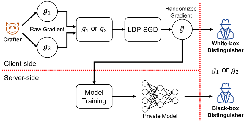
Figure 1(a) shows our empirical privacy measurement that is inspired by the hypothesis tests for measuring the lower bound of central DP (CDP) [36, 19]. The privacy test estimates how an adversary predicts if a reported randomized gradient was crafted from a raw gradient $g_{1}$ or $g_{2}$. To realize such distinguishing game, we introduce crafter and distinguisher. Crafter (maliciously) generates $g_{1}$ and $g_{2}$, then submits a randomized gradient of either one. Distinguisher attempts to discriminate the source of the randomized gradient. The empirical LDP is estimated over sufficient number of games.

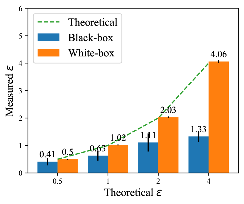
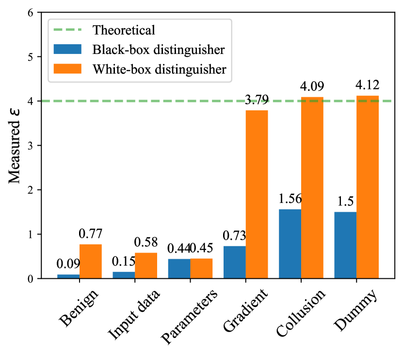
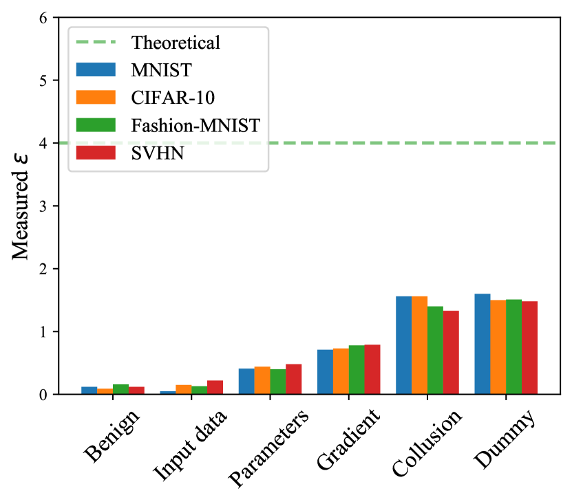
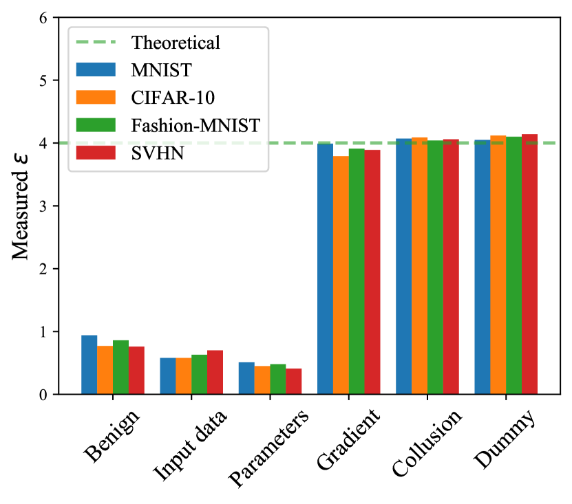
As for the adversary instantiations, the main challenge is to actualize robust adversary attacks against the noise to achieve $\varepsilon$-LDP since the LDP mechanisms tend to inject exetemely larger noise than those of CDP. In addition, we also need to consider collusions between the server and the client. This paper tackles these challenges to realize the way to measure the lower bounds of LDP in FL, and demonstrates the measured $\varepsilon$ ranging from the benign to the worst-case in Figure 1(b).

As a result of our solutions, this paper shows the following four facts: (a) adversaries who directly manipulate raw gradients (i.e., white-box distinguisher) can reach the theoretical upper bounds given by the privacy parameter $\varepsilon$, (b) even in white-box scenarios, the crafters with accessing only the input data and parameters but not the raw gradient have limited capability, (c) the distinguishers with referring only to the updated model but not any randomized gradient (i.e., black-box distinguisher) have limited capability, (d) collusion with the server, like malicious pre-training, increases the adversary’s capability. See the details in section 4.

Contributions. We here summarize our contributions as following three claims:

1. We establish the empirical privacy measurement test of LDP in distributed learning environments.

2. We introduce six types of adversary instantiations that helps practitioners interpret the privacy parameter $\varepsilon$. We also seek the worst-case attack in FL using LDP-SGD.

3. We demonstrate the empirical privacy levels (i.e., lower bounds of LDP) at various attack surfaces defined by the instantiated adversaries.

This study enables us to discuss appropriate privacy levels and their relaxations between the (unrealistic) worst-case scenario and the other weak adversaries. At the end, we also discuss the feasibility of the relaxation with introducing a trusted entity like secure aggregator.

(a) Our privacy measuring test in federated learning.

(b) Measured privacy.

Figure 1: Our (a) privacy test demonstrates (b) empirical LDP against six instantiated adversaries. The test consists of crafter, which generates (malicious) inputs, and distinguisher, which infers the input. The measured privacy is close to the theoretical bound given by $\varepsilon$ when the adversary directly manipulates raw gradients (i.e., white-box distinguisher), resulting in far from the bound otherwise.

Related work. [29, 20, 19, 36] instantiated adversaries in machine learning under CDP. Liu et al.[29] proposed an interpretation of the CDP by means of a hypothesis test. An adversary predicts whether the input data is $D$ or $D^{\prime}$ from the output. They quantified the success of the hypothesis test using precision-recall-relation. Jagielski et al. [19] were the first to attempt an empirical privacy measure using a hypothesis test. They analyzed the privacy level of training models privacy-protected with DP-SGD [1, 2, 40] against membership inference [42] and two poisoning attacks [17, 19]. Nasr et al. [36] showed that theoretical and empirical $\varepsilon$ are tight when a contaminated database is used for training in DP-SGD. As mentioned above, we follow the abstract framework proposed in [36] but address further challenging issues to realize how to measure the lower bounds of LDP in FL. ML Privacy Meter [34] verifies whether a mechanism guarantees privacy, while our study shows how a mechanism that already guarantees $\varepsilon$-LDP can withstand attacks.

2 Preliminaries

This section introduces essential knowledge for understanding our proposal. We first describe local differential privacy. Then, we introduce LDP-SGD, a local privacy mechanism in distributed learning.

2.1 Local Differential Privacy

Definition 1 ($\varepsilon$-Local Differential Privacy).

A randomized algorithm $\mathcal{M}$ satisfies $\varepsilon$-local differential privacy, if and only if for any pair of inputs $x,x^{\prime}\in D$ and for any possible output $S\in Range(\mathcal{M})$:

$$\text{Pr}[\mathcal{M}(x)\in S]\leq e^{\varepsilon}\cdot\text{Pr}[\mathcal{M}(x^{\prime})\in S].$$ (1)

Intuitively, we only obtain the indistinguishable information from $\mathcal{M}$ even when the inputs differ.

Algorithm 1 LDP-SGD; client-side $\mathcal{A}_{\text{client}}$ [10]

0:  Local privacy parameter: $\varepsilon$, current model: $\theta_{t}\in\mathbb{R}^{d}$, $\ell_{2}$-clipping norm: $L$

1:  Compute clipped gradient $x\leftarrow\nabla\ell(\theta_{t};d)\cdot\min\left\{1,\dfrac{L}{||\nabla\ell(\theta_{t};d)||_{2}}\right\}$

2:  $z\leftarrow\begin{cases}L\cdot\frac{x}{||x||_{2}}&\textrm{w.p. }\frac{1}{2}+\frac{||x||_{2}}{2L}\\ -L\cdot\frac{x}{||x||_{2}}&\textrm{otherwise.}\end{cases}$

3:  Sample $v\sim_{u}S^{d}$, the unit sphere in $d$ dims $\hat{z}\leftarrow\begin{cases}\text{sgn}(\langle z,v\rangle)\cdot v&\textrm{w.p. }\frac{e^{\varepsilon}}{1+e^{\varepsilon}}\\ -\text{sgn}(\langle z,v\rangle)\cdot v&\textrm{otherwise.}\end{cases}$

4:  return  $\hat{z}$

Algorithm 2 LDP-SGD; server-side $\mathcal{A}_{\text{server}}$ [10]

0:  Local privacy budget: $\varepsilon$, number of epochs: $T$, parameter set: $C$

1:  $\theta_{0}\leftarrow\{0\}^{d}$

2:  for $t\in[T]$ do

3:     Send $\theta_{t}$ to all clients

4:     $g_{t}\leftarrow\frac{L\sqrt{\pi}}{2}\cdot\frac{\Gamma(\frac{d-1}{2}+1)}{\Gamma(\frac{d}{2}+1)}\cdot\frac{e^{\varepsilon}+1}{e^{\varepsilon}-1}\left(\frac{1}{n}{\sum_{i\in[n]}\hat{z}_{i}}\right)$

5:     Update: ${\theta_{t+1}\leftarrow\prod_{C}(\theta_{t}-\eta_{t}\cdot g_{t})}$,where $\prod_{C}(\cdot)$ is the $\ell_{2}$-projection onto set $C$, and $\eta_{t}=\frac{||C||_{2}\sqrt{n}}{L\sqrt{d}}\cdot\frac{e^{\varepsilon}-1}{e^{\varepsilon}+1}$

6:  end for

7:  return  $\theta_{priv}\leftarrow\theta_{T}$

2.2 Federated Learning using LDP-SGD

Federated learning (FL) [32, 22] is a decentralized machine learning technique. The major difference between traditional machine learning and FL is that client does not share her data with servers or other clients. However, in FL, it is pointed out that the images used in training the model can be restored from their gradients released by clients [14, 43]. One way to prevent the restoration is to randomize gradients for satisfying LDP.

As shown in Figure. 1(a), FL assumed in this paper consists of an untrusted model trainer (server) and clients that own sensitive data. First, the client creates the gradient with the parameters distributed by the model trainer. The client then randomizes the gradient under LDP and sends it to the model trainer. The model trainer updates the parameters with the gradient collected from the client. We randomize the gradient using LDP-SGD (locally differentially private stochastic gradient descent) [8, 10] as described in Algorithm 1 and 2. The client side algorithm (Algorithm 1) performs two gradient randomizations at line 2 and 3. We refer to the line 2 as gradient norm projection and the line 3 as random gradient sampling. We instantiate the adversary based on the following two facts:

• Gradient norm projection (line 2): the smaller the norm of the gradient before randomization, the more likely the sign of the gradient is reversed.

• Random gradient sampling (line 3): the gradient close to the gradient before randomization is likely to be generated when the privacy parameter $\varepsilon$ is set large.

3 Measuring Lower Bounds of LDP

This section describes how to measure the empirical privacy level of FL under LDP.

3.1 Lower Bounding $\varepsilon$ of LDP as Hypothsis Testing

Given a output $y$ of a randomized mechanism $\mathcal{M}$, consider the following hypothesis testing experiment. We choose a null hypothesis as input $x$ and alternative hypothesis as $x^{\prime}$:

$H_{0}$: $y$ came from a input $x$

$H_{1}$: $y$ came from a input $x^{\prime}$

For a choice of a rejection region $S$, the false positive rate(FP), when the null hypothesis is true but rejected, is defined as Pr[$\mathcal{M}(x)\in S$]. The false negative rate(FN), when the null hypothesis is false but retained, is defined as Pr[$\mathcal{M}(x^{\prime})\in\bar{S}$] where $\bar{S}$ is the complement of $S$. Mechanism $\mathcal{M}$ satisfying $\varepsilon$-LDP is equivalent to satisfying the following conditions[21].

Theorem 1 (Empirical $\varepsilon$-Local Differential Privacy).

For any $\varepsilon\in\mathbb{R}^{+}$, a randomized mechanism $\mathcal{M}$ is $\varepsilon$-differentially private if and only if the following conditions are satisfied for all pairs of input values $x$ and $x^{\prime}$, and all rejection region $S\subseteq Range(\mathcal{M})$:

$$\begin{split}\text{Pr}[\mathcal{M}(x)\in S]+e^{\varepsilon}\cdot\text{Pr}[\mathcal{M}(x^{\prime})\in\bar{S}]&\geq 1,and\\ e^{\varepsilon}\cdot\text{Pr}[\mathcal{M}(x)\in S]+\text{Pr}[\mathcal{M}(x^{\prime})\in\bar{S}]&\geq 1.\end{split}$$ (2)

Therefore, we can determine the empirical $\varepsilon$-local differential privacy as

$$\varepsilon_{\text{empirical}}=\max\left({\log\dfrac{1-\text{FP}}{\text{FN}},\log\dfrac{1-{\text{FN}}}{\text{FP}}}\right)$$ (3)

For example, in 100 trials, suppose the false-positive rate, when the actual input was $x$ but the distinguisher guesses $x^{\prime}$, was 0.1, and the false-negative rate, when the actual input was $x^{\prime}$ but the distinguisher guesses $x$, was 0.2. Substitute in FP and FN in Equation 3 to obtain $\varepsilon_{\text{empirical}}\fallingdotseq 2.0$.

3.2 Instantiating the LDP Adversary in FL

To perform the privacy test based on the above hypothesis testing, we define the following entities:

• Crafter produces two gradients, $g_{1}$ and $g_{2}$, with the global model $\theta_{t}$, corresponding to a malicious client in FL. This entity honestly randomizes one of gradients by Algorithm 1 and makes it $\tilde{g}$. $\tilde{g}$ is sent to the model trainer and distinguisher.

• Model trainer uses the $\tilde{g}$ received from the crafter to update the global model $\theta_{t}$ to $\theta_{t+1}$ by Algorithm 2. This entity corresponds to a untrusted server in FL.

• Distinguisher predicts whether the randomized gradient was $g_{1}$ or $g_{2}$. This entity has the data $x_{1}$, $x_{2}$ that the crafter used to generate the gradient.

We divide the distinguisher into two classes, black-box distinguisher and white-box distinguisher. For each distinguisher, we propose two different privacy measurement tests, namely, black-box LDP test (Algorithm 3) and white-box LDP test (Algorithm 4).

Algorithm 3 Black-box LDP Test in FL

0:  Privacy parameter: $\varepsilon$, $\#$trials: $K$

1:  for $k\in[K]$ do

2:     Model trainer sends $\theta_{t}$ to crafter.

3:     Crafter

4:        $\{g_{1},g_{2}\}\leftarrow\text{Craft}(x_{1},x_{2},\theta_{t})$

5:        Randomly choose $g$ from $\{g_{1},g_{2}\}$.

6:        $\tilde{g}\leftarrow\mathcal{A}_{\text{client}}(g)$.

7:        Submit $\tilde{g}$ to model trainer.

8:        Share $x_{1}$, $x_{2}$, $\theta_{t}$ w/ distinguisher

9:     Model Trainer

10:        $\theta_{t+1}\leftarrow\mathcal{A}_{\text{server}}(\theta_{t})$

11:        Submit $\theta_{t+1}$ to distinguisher

12:     Distinguisher

13:        $\text{guess}\leftarrow\mathcal{D}_{\text{black}}(\theta_{t+1},\theta_{t},x_{1},x_{2})$

14:  end for

15:  Compute $\varepsilon_{\text{empirical}}$ as (3)

Algorithm 4 White-box LDP Test in FL

0:  Privacy parameter: $\varepsilon$, $\#$trials: $K$

1:  for $k\in[K]$ do

2:     Model trainer sends $\theta_{t}$ to crafter.

3:     Crafter

4:        $\{g_{1},g_{2}\}\leftarrow\text{Craft}(x_{1},x_{2},\theta_{t})$

5:        Randomly choose $g$ from $\{g_{1},g_{2}\}$

6:        $\tilde{g}\leftarrow\mathcal{A}_{\text{client}}(g)$.

7:        Submit $\tilde{g}$ to distinguisher.

8:        Share $g_{1}$, $g_{2}$ w/ distinguisher.

9:     Distinguisher

10:        $\text{guess}\leftarrow\mathcal{D}_{\text{white}}(\tilde{g},g_{1},g_{2})$

11:  end for

12:  Compute $\varepsilon_{\text{empirical}}$ as (3)

3.3 Dinstinguisher Algorithms

Black-box Distinguisher.

Let black-box distinguisher $\mathcal{D}_{\text{black}}$ be the distinguisher that cannot access the randomized gradient, but can access the global parameters $\theta_{t+1}$ updated with using it. That is, the black-box disntinguisher only observes the updates after each step of federated learning, but not see any details of inner process of the federated learning. For simplicity’s sake, we only consider the global model is updated using a single randomized gradient. The black-box distinguisher predicts the randomized gradient by computing the loss of $x_{1}$ (and $x_{2}$), then compare the differences before and after the model update. By default, the distinguisher $\mathcal{D}_{\text{black}}$ employs the following inference against two choices:

$$guess=\begin{cases}{g_{1}}&f(x_{1};\theta_{t+1})\leq f(x_{1};\theta_{t})\\ {g_{2}}&otherwise\end{cases}.$$ (4)

This is based on that $g_{2}$ aims to degrade the model. However, the inference does not work well for all crafters. In section 3.4, we mention about the replacement for the inequality.

White-box Distinguisher.

White-box distinguisher $\mathcal{D}_{\text{white}}$ directly accesses a single randomized gradient $\tilde{g}$. In addition, the white-box distinguisher can generate two raw gradients $g_{1}$ and $g_{2}$ as well as the client, then computes the similarity between $\tilde{g}$ and the raw gradients to estimate the origin of the $\tilde{g}$. Here, we employ the cosine similarity between $\tilde{g}$ and $\{g_{1},g_{2}\}$. The discrimination by the white-box distinguisher is defined as follows:

$$guess=\begin{cases}{g_{1}}&cos(\tilde{g},g_{1})\geq cos(\tilde{g},g_{2})\\ {g_{2}}&otherwise\end{cases}.$$ (5)

3.4 Crafter Algorithms

We propose several types of adversaries depending on the access level. We introduce six types of crafter algorithms Craft($\cdot$) in Algorithm 3 and 4. One crafter algorithm assumes collusion with the model trainer. The adversary setting proposed in this paper is summarized in Table 1.

Table 1: Adversary settings. The lower the row, the stronger (i.e. more unrealistic) the adversary.

Adversary	Malicious Access		Distinguisher
	Crafter	Model trainer	Black-box	White-box
Benign	Benign.	Benign.	Eq. (6)	Eq. (5)
Input perturbation	Images.	Benign.	Eq. (4)	Eq. (5)
Parameter retrogression	Parameters.	Benign.	Eq. (4)	Eq. (5)
Gradient flip	Gradients.	Benign.	Eq. (4)	Eq. (5)
Collusion	Gradients	Parameters.	Eq. (4)	Eq. (5)
Dummy gradient	Gradients.	Benign.	Eq. (7)	Eq. (5)

Benign setting. As the most realistic setting, suppose all entities are benign. In the benign setting, the crafter uses the global model $\theta_{t}$ distributed by the model trainer to generate gradients $g_{1}$ and $g_{2}$ from the images $x_{1}$ and $x_{2}$. Thus, the two gradients are also crafted without malicious behaviors as:

$$g_{1}=\nabla f(x_{1},\theta_{t}); g_{2}=\nabla f(x_{2},\theta_{t})$$

In this scenario, the black-box distinguisher considers the reported randomized gradient as $g_{1}$ if

$$\delta(x_{1})\geq\delta(x_{2})\ \text{where}\ \delta(x)=|f(x;\theta_{t+1})-f(x;\theta_{t})|.$$ (6)

otherwise $g_{2}$.

Input perturbation. This scenario assumes that the crafter produces malicious input data via perturbations. The crafter adds perturbation to the data $x_{1}$ to make it easier to distinguish the gradient. Although many studies have proposed perturbation algorithms [38, 33, 39, 6, 13], we adopted the FGSM (Fast Gradient Sign Method) [16], a well-known method for adversarial perturbations. For an input image, FGSM uses the gradients of the loss with respect to the input image to create a new image that maximizes the loss. Let $x_{2}$ be an adversary pertubed image crafted as $x_{2}=x_{1}+\alpha\ \text{sgn}(\nabla_{x_{1}}f(x_{1};\theta_{t}))$ .

Parameter retrogression. Let us assume that the crafter has maliciously manipulated the parameters [35]. Generating a gradient from manipulated parameters results in a significant difference in norm compared to generating it from benign parameters. This setup suggests the ease of distinguishing between two gradients with very different norms. Let $\theta_{t}^{\prime}$ be the parameter updated in the direction of increasing $x_{1}$ loss as $\theta_{t}^{\prime}=\theta_{t}+\alpha\ \nabla f(x_{1};\theta_{t})$. Generate gradients $g_{1}$ from the benign parameter $\theta_{t}$ and $g_{2}$ from the retrograded parameter $\theta_{t}^{\prime}$.

$$g_{1}=\nabla f(x_{1},\theta_{t}); g_{2}=\nabla f(x_{1},\theta_{t}^{\prime})$$

Gradient flip. In this setting, the crafter processes the raw gradient. The simplest method of processing a gradient to increase its discriminability is to flip the gradient sign [35]. As described in Section 2.2, in the random gradient sampling of LDP-SGD, when $\varepsilon$ is set large, the sign of the gradient is unlikely to change, so we argue that such processing is effective. The crafter uses the global model $\theta_{t}$ distributed by the model trainer to generate gradients $g_{1}$ from the image $x_{1}$. Let $g_{2}$ be a gradient with the sign of $g_{1}$ flipped.

$$g_{1}=\nabla f(x_{1},\theta_{t}); g_{2}=-g_{1}$$

Collusion. We here consider distributing a malicious model from the server to the clients. As explained in Section 2.2, in the gradient norm projection of LDP-SGD, the smaller the norm of the raw gradient, the easier it is for the sign to be flipped. Taking advantage of this property, we consider a setting where the crafter and the model trainer collude to make generating a gradient with a small norm challenging. With this setting, the model trainer intentionally creates a global model with a massive loss and distributes it to the crafter. The crafter flips a gradient in the same way as the gradient flipping. Thus the gradient $g_{2}$ is generated as $g_{2}=-g_{1}$. As a realization of this adversary, we introduce the following procedure. First the model trainer generates a malicious global model $\tilde{\theta}_{t}$ from only images with the same label and distribute it to the crafter. Second, the crafter utilizes the malicious model $\tilde{\theta}_{t}$ to generate gradients $g_{1}$ from the image $x_{1}$. The label of $x_{1}$ is different from the label of the images used to generate the malicious model.

$$g_{1}=\nabla f(x_{1},\tilde{\theta}_{t}); \textrm{where }\tilde{\theta}_{t}\textrm{ is a malicious model.}$$

As well as the gradient flip, the adversary craft $g_{2}$ by flipping $g_{1}$.

Dummy gradient. Here, we consider that the crafter produces a dummy gradient. LDP-SGD includes the gradient norm projection, which causes errors due to randomly flipping gradients. The intuition here is to craft a dummy gradient that never cause such errors. The simplest way to do this is to generate a gradient with a large norm, regardless of the image or model the crafter has. To craft the dummy gradient, we simply fill a constant $\lambda$ into all the elements of the gradient as:

$$g_{1}=(\lambda,\lambda,\dots,\lambda);$$

The norm of $g_{1}$ must be greater than or equal to the clipping threshold $L$ to avoid the gradient norm projection. Therefore, let $\lambda$ be $L/\sqrt{d}$ and $d$ be the dimension of the gradient. For another choice of the gradient, we also employ the gradient flipping to maximize the difference against the dummy gradient. Thus the gradient $g_{2}$ is generated as $g_{2}=-g_{1}$ as well. In this scenario, the black-box distinguisher considers the reported randomized gradient as $g_{1}$ if

$$\sum_{i\in[d]}\text{sgn}(\theta^{i}_{t+1}-\theta^{i}_{t})\geq 0,$$ (7)

otherwise $g_{2}$. This is due to that the crafter produces the dummy gradient $g_{1}$ by filling the positive constant. The combination of crafting the dummy gradient and flipping it is a worst-case attack for the LDP adversary. We give a proof below.

3.5 Analysis of the Worst-case Attack

In the above adversary instatiations with the crafter and the distinguisher, we can find a worst-case attack in FL using LDP-SGD. About the worst-case, we meet the following proposition.

Proposition 1.

The white-box distinguisher with the crafter producing a raw gradient whose $\ell_{2}$-norm is larger than or equal to $L$ is a worst-case attack reaching the theoretical upper bound given by $\varepsilon$.

Proof.

Recall that in LDP-SGD, the direction is reversed depending on the gradient norm and $\varepsilon$. First, since the sign is easily flipped when the norm of the gradient is small in the gradient norm projection, the norm of the gradient must be greater than or equal to $L$. Hereafter, we assume that $g$ is a gradient with norm $L$. Let $g_{\text{flip}}$ be the flipped gradient of $g$, $\tilde{g}$ and $\tilde{g}_{\text{flip}}$ be the outputs of the random gradient sampling, respectively. With probability of $\frac{e^{\varepsilon}}{1+e^{\varepsilon}}$, the following equation holds on line 3.

$$g\cdot\tilde{g}\geq 0 \quad g_{\text{flip}}\cdot\tilde{g}_{\text{flip}}\geq 0$$

Let $\tilde{g}_{\text{target}}$ be the gradient randomized of either $g$ or $g_{\text{flip}}$ with probability of $50\%$. Let us predict what $g_{\text{target}}$ be. The case can be divided by the cosine similarity between $\tilde{g}_{\text{target}}$ and $g$ as follows:

$$cos(\tilde{g}_{\text{target}},g)\geq 0 \Rightarrow \begin{cases}g_{\text{target}}\textrm{ was }g\textrm{ and }g\textrm{ rotation was within 90 degrees.}&\textrm{ w.p. }\frac{1}{2}\cdot\frac{e^{\varepsilon}}{1+e^{\varepsilon}}\\ g_{\text{target}}\textrm{ was }g_{\text{flip}}\textrm{ and }g_{\text{flip}}\textrm{ rotation was over 90 degrees.\;\;}&\textrm{ w.p. }\frac{1}{2}\cdot\frac{1}{1+e^{\varepsilon}}\end{cases}$$

$$cos(\tilde{g}_{\text{target}},g)\leq 0 \Rightarrow \begin{cases}g_{\text{target}}\textrm{ was }g\textrm{ and }g\textrm{ rotation was over 90 degrees.}&\textrm{w.p. }\frac{1}{2}\cdot\frac{1}{1+e^{\varepsilon}}\\ g_{\text{target}}\textrm{ was }g_{\text{flip}}\textrm{ and }g_{\text{flip}}\textrm{ rotation was within 90 degrees.}&\textrm{w.p. }\frac{1}{2}\cdot\frac{e^{\varepsilon}}{1+e^{\varepsilon}}\end{cases}$$

White-box distinguisher predicts $g$ for the original data of $\tilde{g}_{\text{target}}$ when the cosine similarity between $g$ and $\tilde{g}_{\text{target}}$ is positive, then the prediction is correct with probability $\frac{1}{2}\cdot\frac{e^{\varepsilon}}{1+e^{\varepsilon}}$. Likewise, white-box distinguisher predicts $g_{\text{flip}}$ for the original data of $\tilde{g}_{\text{target}}$ when the cosine similarity between $g$ and $\tilde{g}_{\text{target}}$ is negative, then the prediction is correct with probability $\frac{1}{2}\cdot\frac{e^{\varepsilon}}{1+e^{\varepsilon}}$. Therefore, white-box distinguisher can distinguish $g$ and $g_{\text{flip}}$ with probability $\frac{e^{\varepsilon}}{1+e^{\varepsilon}}$. ∎

4 Numerical Observations

Here, we address an experimental study to observe numerical results of our LDP tests in FL.

4.1 Experimental Setup

For each adversary instantiations listed in Table 1, we run ten measurements and average over these measurement results. Each measurement consists of $K$=10,000 trials by each distinguisher.

Hyper-parameters. We have implemented our algorithms in Pytorch. For each dataset, we used cross-entropy as loss function. We used three layers convolutional neural network for all datasets. To train the models, we use LDP-SGD [10] with clipping norm size $L$=1. Guaranteed privacy level $\varepsilon$ is set to 0.5, 1.0, 2.0 and 4.0.

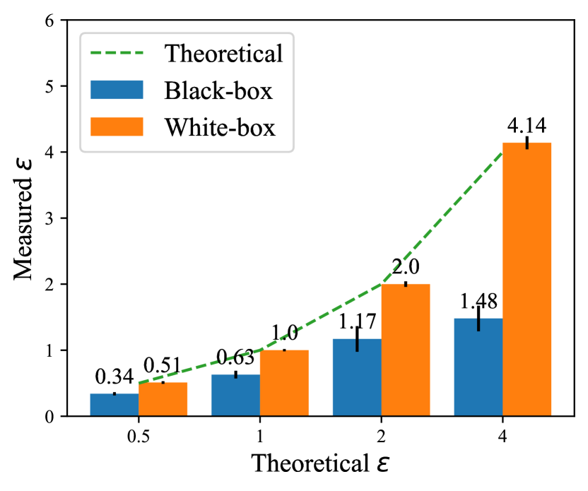
Datasets. We perform experimental evaluations on four datasets, namely MNIST [26], CIFAR-10 [25], Fashion-MNIST [41] and SVHN [37]. Detail results of CIFAR-10, Fashion-MNIST and SVHN are in Appendix.

(a) Benign setting

(b) Image perturbation

(c) Parameter retrogression

(d) Gradient flip

(e) Collusion

(f) Dummy gradient

Figure 2: The empirical privacy in federated learning. (MNIST)

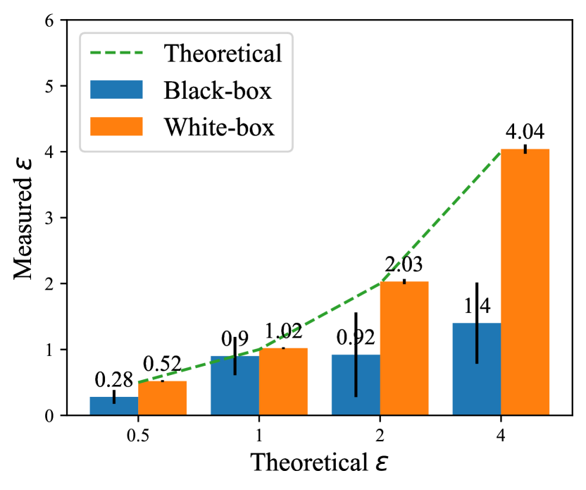
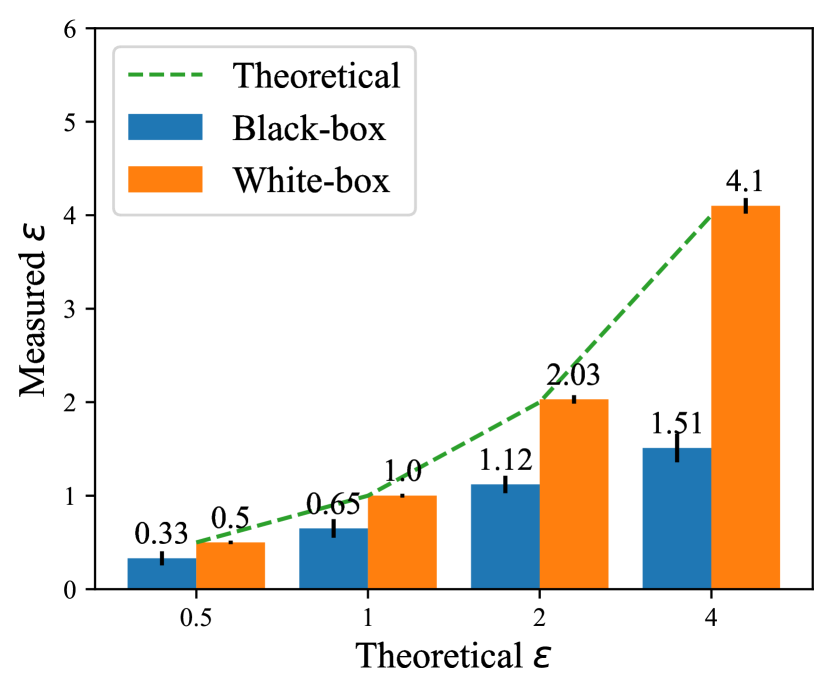
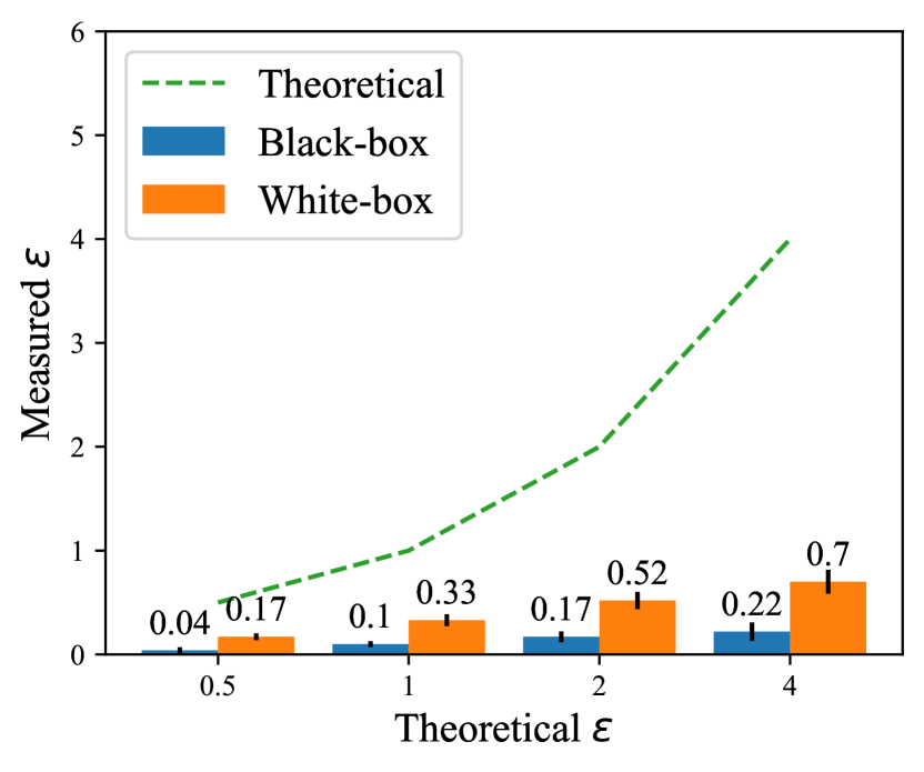
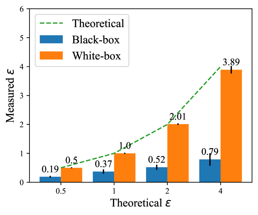
4.2 Observations of Empirical LDP

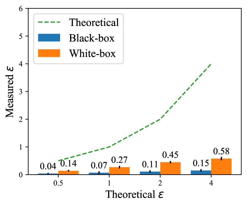
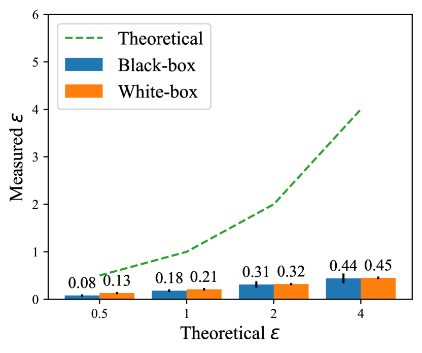
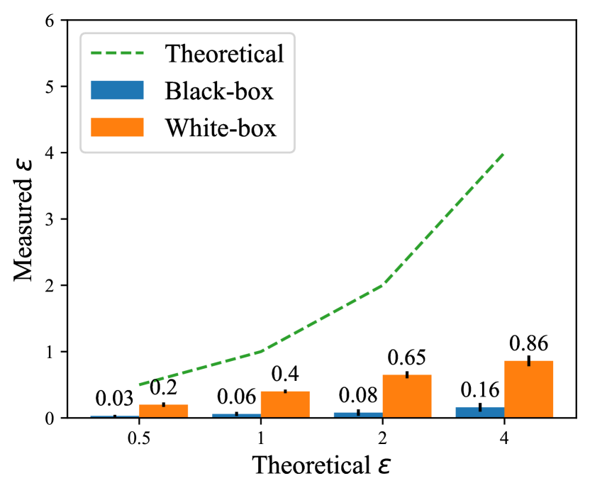
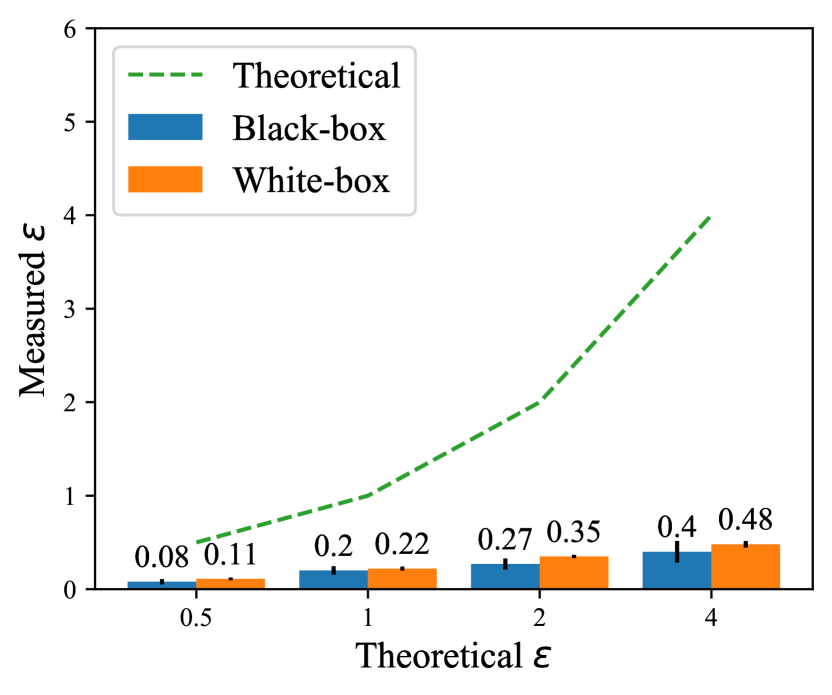
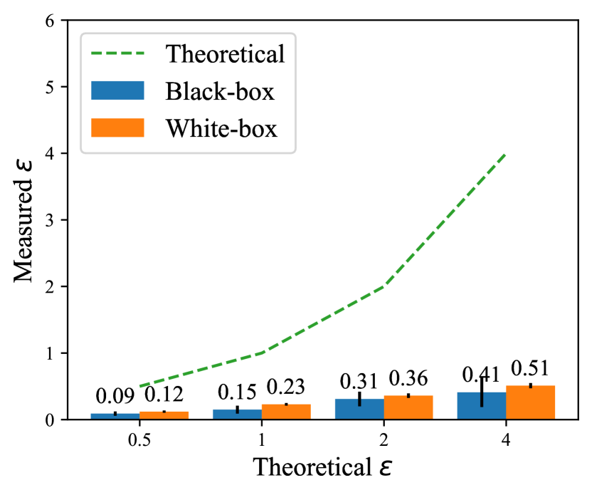
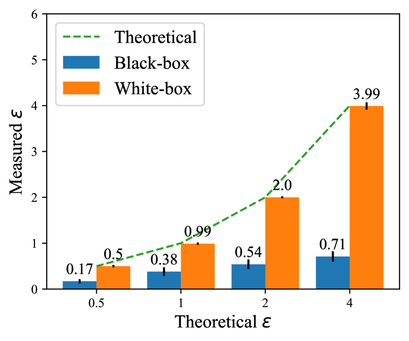
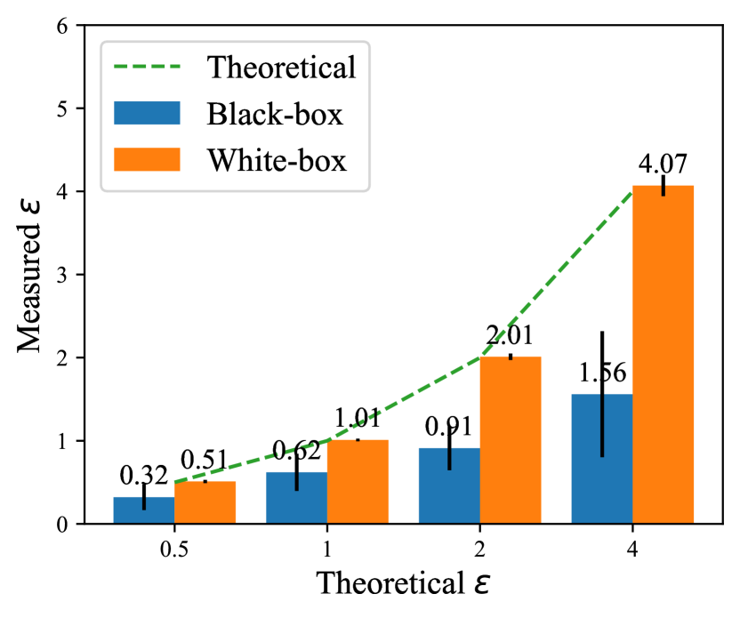
Figure 2 shows the measured $\varepsilon$ ($\varepsilon_{\text{empirical}}$) by our LDP test varying the privacy parameter $\varepsilon$.

Benign. In this most realistic setting, even if we set $\varepsilon=4$, the empirical privacy strength is $0.94$, and the gap between the theoretical and the empirical is large. (Figure 2(a)) $\varepsilon_{\text{empirical}}=0.94$ is equivalent to about $68.1\%$ in terms of the identifiable probability. White-box distinguisher has a higher $\varepsilon_{\text{empirical}}$ than black-box distinguisher. Therefore it is easier to determine the randomized gradient $\tilde{g}$ itself than the parameter $\theta_{t+1}$ updated with the randomized gradient $\tilde{g}$.

Input perturbation. From Figure 2(b), the probability of discrimination does not increase even if the gradient of the perturbed image is randomized. The gap between empirical and theoretical privacy strength in this setting is more expansive than in the benign setting. Therefore, even if the image changes slightly due to perturbation, the gradient will not be easy to distinguish.

Parameter retrogression. In this setup, we use a nonmalicious gradient $g_{1}$ and a $g_{2}$ generated from parameters that have been processed to increase loss. Since the norm of $g_{2}$ is larger than the norm of $g_{1}$, we assume that discrimination would be easier if it were not randomized. However, Figure 2(c) shows that the gradient norm has a negligible effect on the discrimination probability. This result is that in LDP-SGD, gradient clipping keeps large normed gradients below a threshold.

Gradient flip. The measured $\varepsilon$ is shown in Figure 2(d). Discriminability was improved compared to the benign setting when the crafter flipped the gradient sign. In particular, when $\varepsilon=4$, $\varepsilon_{\text{empirical}}$ shows 3.99, almost a theoretical value in white-box distinguisher. As shown in the worst-case proof, LDP-SGD keeps the direction roughly proportional to the guaranteed $\varepsilon$, so $g_{1}$ and $g_{2}$, which reverses the sign of $g_{1}$, are easy to distinguish.

Collusion. The experimental results in Figure 2(e) show that the collusion between the crafter and the model trainer narrows the gap between theoretical privacy and empirical privacy compared to the gradient flipping. In white-box distinguisher of this setting, the empirical $\varepsilon$ reached the theoretical value at all the setting values $\varepsilon=0.5,1,2,4$. $\varepsilon_{\text{empirical}}=4.07$ has the same meaning as successful discrimination with a probability of about $98.2\%$. In the black-box setting, this collusion increased the empirical LDP against the weaker settings described in the above paragraphs.

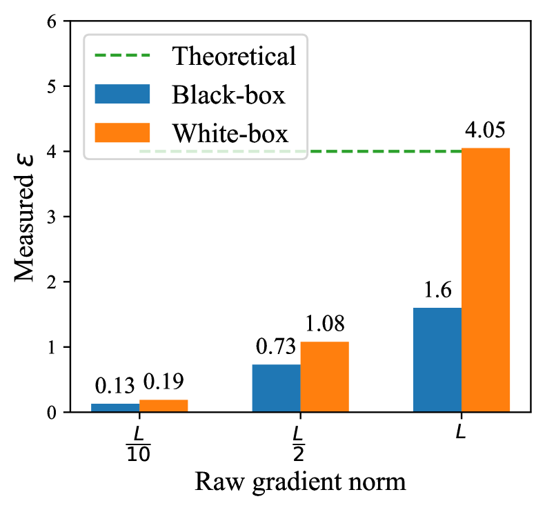
Dummy gradient. From Figure 2(f), as with the collusion, this setting increases the probability of gradient discrimination. Figure 4 shows the effect of the norm on the discrimination probability: even with a dummy gradient, if the norm is smaller than the clipping size $L$, the gap between the theoretical and measured $\varepsilon$ becomes larger. Daring to generate the dummy gradients with large norm is not common in FL. However, it is clear that maximizing the norm of the gradient and sign flipping is the strongest attack.

Summary of Results. Figure 1(b), 4(a), and 4(b) summarizes the results for each dataset. Over the four datasets, adversaries who directly manipulate raw gradients can reach the theoretical upper bounds given by the privacy parameter $\varepsilon$. Even in white-box scenarios, adversaries who only access the input data and parameters but not the raw gradient have limited capability. Moreover, adversaries who only refer to the updated model but not any randomized gradient (i.e., black-box scenarios) have the limited capability, collusion with the server employing the malicious model, increases the adversary’s capability in the black-box setting.

Figure 3: Effect of gradient norm.

(a) Black-box

(b) White-box

Figure 4: Summary of results in four datasets.

4.3 Discussion towards Relaxations of Privacy Parameters

The white-box test resulted in tightly close to the theoretical bound defined by the privacy parameters $\varepsilon$. While the black-box test demonstrated stronger privacy levels that were far from the bound. To prevent the white-box attacks, we can install a secure aggregator based on such as multi-party computations and trusted execution environments (TEEs) [31, 7]. Using such secure aggregators for updating the global model, the process from reporting gradients to updating the global model is fully encrypted. The experimental results above do not allow any relaxation only with local randomizers, but with shuffler [4, 9, 12, 28] or aggregator implemented by such secure computations [5, 24], relaxation of $\varepsilon$ can be reasonable in the view of empirical privacy risks. Even when the shuffler is untrusted and the gradient is randomized with a relaxed privacy parameter (like $\varepsilon=8$), the empirical privacy risk against the shuffler might not be significant (like $\varepsilon_{\text{empirical}}=1$). Another possible way is to prohibit gradient poisoning. As shown in the experiments, without directly manipulating gradients, the empirical privacy is significantly far from the given privacy bound. If the range of possible input training data is limited, we can introduce out-of-distribution detectors before randomizing raw gradients. In other words, by adding some restrictions to the crafter, the model trainer, and the distinguisher, it may also be possible to relax $\varepsilon$.

5 Conclusion

We introduced the empirical privacy test by measuring the lower bounds of LDP. We then instantiated six adversaries in FL under LDP to measure empirical LDP at various attack surfaces, including the worst-case attack that reached the theoretical upper bound of LDP. We also demonstrated numerical observations of the measured privacy in these adversarial settings. In the end, we discussed the possible relaxation of privacy parameter $\varepsilon$ with using a trusted entity.

Appendix A Experimental Details

This appendix provides details of the setup and additional experimental results.

A.1 Experimental Setup

Datasets. We run experiments on four datasets:

• MNIST: We use the MNIST image dataset, which consists of 28$\times$28 handwritten grayscale digit images, and the task is to recognize the 10 class digits.

• CIFAR-10: We use CIFAR10, a standard benchmark dataset consisting of 32$\times$32 RGB images. The learning task is to classify the images into ten classes of different objects.

• Fashion-MNIST: Each example of Fashion-MNIST is a 28$\times$28 grayscale image associated with a label from 10 classes.

• SVHN: This dataset is obtained from house numbers in Google Street View images. SVHN consists of 32$\times$32 RGB images, and the task is to recognize the 10 class digits.

Neural Network Architecture. The neural network we use in the experiments is as in Table 3.

Table 2: Neural network architecture in measurements.

Layer	Parameters
Convolution	16 filters of 8$\times$8, strides 2
Max-Pooling	2$\times$2 window, strides 2
Convolution	32 filters of 4$\times$4, strides 2
Max-Pooling	2$\times$2 window, strides 2
Linear	32 units
Softmax	10 units

Table 3: The black-box test for multiple clients in the benign crafter. (MNIST)

Number of clients	Measured $\varepsilon$
1	0.12
2	0.07
4	0.06
10	0.06

A.2 Additional Observations

Dataset Perspectives. Figure 5, 6 and 7 show that the empirical privacy in federated learning in CIFAR-10, Fashion-MNIST, and SVHN datasets. The observation of $\varepsilon_{\text{empirical}}$ using four datasets shows that $\varepsilon_{\text{empirical}}$ is data-independent and has a similar trend. As in Section 4.2, the white-box LDP test is more potent than the black-box LDP test. Furthermore, the craft of dummy gradients is closest to the theoretical $\varepsilon$.

White-box test showed higher $\varepsilon_{\text{empirical}}$ than black-box test. This is a natural result in black-box scenarios since the model trainer aggregate gradients such as averaging, learning rate multiplication, and $\ell_{2}$-projection. The more clients used to update parameters in FL, the more pronounced this trend becomes. Table 3 shows that the black-box test for multiple clients becomes more difficult as the number of clients increases.

Input perturbation and parameter retrogression were not successful. As mentioned in Section 2.2, LDP-SGD includes the clipping gradient and the random gradient sampling. The clipping gradient ignores large differences between the norms of $g_{1}$ and $g_{2}$. Furthermore, the random gradient sampling rotates the gradient by at most 90 degrees, so any slight difference in the direction of $g_{1}$ and $g_{2}$ is ignored.

(a) Benign setting

(b) Image perturbation

(c) Parameter retrogression

(d) Gradient flip

(e) Collusion

(f) Dummy gradient

Figure 5: The empirical privacy in federated learning. (CIFAR-10)

(a) Benign setting

(b) Image perturbation

(c) Parameter retrogression

(d) Gradient flip

(e) Collusion

(f) Dummy gradient

Figure 6: The empirical privacy in federated learning. (Fashion-MNIST)

(a) Benign setting

(b) Image perturbation

(c) Parameter retrogression

(d) Gradient flip

(e) Collusion

(f) Dummy gradient

Figure 7: The empirical privacy in federated learning. (SVHN)

References

- Abadi et al. [2016] Martin Abadi, Andy Chu, Ian Goodfellow, H Brendan McMahan, Ilya Mironov, Kunal Talwar, and Li Zhang. Deep learning with differential privacy. In Proceedings of the 2016 ACM SIGSAC conference on computer and communications security, pages 308–318, 2016.
- Bassily et al. [2014] Raef Bassily, Adam Smith, and Abhradeep Thakurta. Private empirical risk minimization: Efficient algorithms and tight error bounds. In 2014 IEEE 55th Annual Symposium on Foundations of Computer Science, pages 464–473. IEEE, 2014.
- Bhowmick et al. [2018] Abhishek Bhowmick, John Duchi, Julien Freudiger, Gaurav Kapoor, and Ryan Rogers. Protection against reconstruction and its applications in private federated learning. arXiv preprint arXiv:1812.00984, 2018.
- Bittau et al. [2017] Andrea Bittau, Úlfar Erlingsson, Petros Maniatis, Ilya Mironov, Ananth Raghunathan, David Lie, Mitch Rudominer, Ushasree Kode, Julien Tinnes, and Bernhard Seefeld. Prochlo: Strong privacy for analytics in the crowd. In Proceedings of the 26th Symposium on Operating Systems Principles, pages 441–459, 2017.
- Bonawitz et al. [2017] Keith Bonawitz, Vladimir Ivanov, Ben Kreuter, Antonio Marcedone, H Brendan McMahan, Sarvar Patel, Daniel Ramage, Aaron Segal, and Karn Seth. Practical secure aggregation for privacy-preserving machine learning. In proceedings of the 2017 ACM SIGSAC Conference on Computer and Communications Security, pages 1175–1191, 2017.
- Carlini and Wagner [2017] Nicholas Carlini and David Wagner. Adversarial examples are not easily detected: Bypassing ten detection methods. In Proceedings of the 10th ACM workshop on artificial intelligence and security, pages 3–14, 2017.
- Costan and Devadas [2016] Victor Costan and Srinivas Devadas. Intel sgx explained. Cryptology ePrint Archive, 2016.
- Duchi et al. [2018] John C Duchi, Michael I Jordan, and Martin J Wainwright. Minimax optimal procedures for locally private estimation. Journal of the American Statistical Association, 113(521):182–201, 2018.
- Erlingsson et al. [2019] Úlfar Erlingsson, Vitaly Feldman, Ilya Mironov, Ananth Raghunathan, Kunal Talwar, and Abhradeep Thakurta. Amplification by shuffling: From local to central differential privacy via anonymity. In Proceedings of the Thirtieth Annual ACM-SIAM Symposium on Discrete Algorithms, pages 2468–2479. SIAM, 2019.
- Erlingsson et al. [2020] Úlfar Erlingsson, Vitaly Feldman, Ilya Mironov, Ananth Raghunathan, Shuang Song, Kunal Talwar, and Abhradeep Thakurta. Encode, shuffle, analyze privacy revisited: Formalizations and empirical evaluation. arXiv preprint arXiv:2001.03618, 2020.
- Evfimievski et al. [2003] Alexandre Evfimievski, Johannes Gehrke, and Ramakrishnan Srikant. Limiting privacy breaches in privacy preserving data mining. In Proceedings of the twenty-second ACM SIGMOD-SIGACT-SIGART symposium on Principles of database systems, pages 211–222, 2003.
- Feldman et al. [2022] Vitaly Feldman, Audra McMillan, and Kunal Talwar. Hiding among the clones: A simple and nearly optimal analysis of privacy amplification by shuffling. In 2021 IEEE 62nd Annual Symposium on Foundations of Computer Science (FOCS), pages 954–964. IEEE, 2022.
- Ford et al. [2019] Nic Ford, Justin Gilmer, Nicolas Carlini, and Dogus Cubuk. Adversarial examples are a natural consequence of test error in noise. arXiv preprint arXiv:1901.10513, 2019.
- Geiping et al. [2020] Jonas Geiping, Hartmut Bauermeister, Hannah Dröge, and Michael Moeller. Inverting gradients-how easy is it to break privacy in federated learning? Advances in Neural Information Processing Systems, 33:16937–16947, 2020.
- Girgis et al. [2021] Antonious Girgis, Deepesh Data, Suhas Diggavi, Peter Kairouz, and Ananda Theertha Suresh. Shuffled model of differential privacy in federated learning. In International Conference on Artificial Intelligence and Statistics, pages 2521–2529. PMLR, 2021.
- Goodfellow et al. [2014] Ian J Goodfellow, Jonathon Shlens, and Christian Szegedy. Explaining and harnessing adversarial examples. arXiv preprint arXiv:1412.6572, 2014.
- Gu et al. [2017] Tianyu Gu, Brendan Dolan-Gavitt, and Siddharth Garg. Badnets: Identifying vulnerabilities in the machine learning model supply chain. arXiv preprint arXiv:1708.06733, 2017.
- Hoshino [2020] Nobuaki Hoshino. A firm foundation for statistical disclosure control. Japanese Journal of Statistics and Data Science, 3, 08 2020. doi: 10.1007/s42081-020-00086-9.
- Jagielski et al. [2020] Matthew Jagielski, Jonathan Ullman, and Alina Oprea. Auditing differentially private machine learning: How private is private sgd? Advances in Neural Information Processing Systems, 33:22205–22216, 2020.
- Jayaraman and Evans [2019] Bargav Jayaraman and David Evans. Evaluating differentially private machine learning in practice. In 28th USENIX Security Symposium (USENIX Security 19), pages 1895–1912. USENIX Association, 2019.
- Kairouz et al. [2015] Peter Kairouz, Sewoong Oh, and Pramod Viswanath. The composition theorem for differential privacy. In International conference on machine learning, pages 1376–1385. PMLR, 2015.
- Kairouz et al. [2021] Peter Kairouz, H Brendan McMahan, Brendan Avent, Aurélien Bellet, Mehdi Bennis, Arjun Nitin Bhagoji, Kallista Bonawitz, Zachary Charles, Graham Cormode, Rachel Cummings, et al. Advances and open problems in federated learning. Foundations and Trends® in Machine Learning, 14(1–2):1–210, 2021.
- Kasiviswanathan et al. [2011] Shiva Prasad Kasiviswanathan, Homin K Lee, Kobbi Nissim, Sofya Raskhodnikova, and Adam Smith. What can we learn privately? SIAM Journal on Computing, 40(3):793–826, 2011.
- Kato et al. [2022] Fumiyuki Kato, Yang Cao, and Masatoshi Yoshikawa. Olive: Oblivious and differentially private federated learning on trusted execution environment. arXiv preprint arXiv:2202.07165, 2022.
- [25] Alex Krizhevsky, Vinod Nair, and Geoffrey Hinton. Cifar-10 (canadian institute for advanced research). URL http://www.cs.toronto.edu/~kriz/cifar.html.
- LeCun and Cortes [2010] Yann LeCun and Corinna Cortes. MNIST handwritten digit database. 2010. URL http://yann.lecun.com/exdb/mnist/.
- Lee and Clifton [2011] Jaewoo Lee and Chris Clifton. How much is enough? choosing for differential privacy. In International Conference on Information Security, pages 325–340. Springer, 2011.
- Liew et al. [2022] Seng Pei Liew, Tsubasa Takahashi, Shun Takagi, Fumiyuki Kato, Yang Cao, and Masatoshi Yoshikawa. Network shuffling: Privacy amplification via random walks. arXiv preprint arXiv:2204.03919, 2022.
- Liu et al. [2019] Changchang Liu, Xi He, Thee Chanyaswad, Shiqiang Wang, and Prateek Mittal. Investigating statistical privacy frameworks from the perspective of hypothesis testing. Proceedings on Privacy Enhancing Technologies, 2019:233–254, 07 2019. doi: 10.2478/popets-2019-0045.
- Liu et al. [2020] Ruixuan Liu, Yang Cao, Masatoshi Yoshikawa, and Hong Chen. Fedsel: Federated sgd under local differential privacy with top-k dimension selection. In International Conference on Database Systems for Advanced Applications, pages 485–501. Springer, 2020.
- McKeen et al. [2013] Frank McKeen, Ilya Alexandrovich, Alex Berenzon, Carlos V Rozas, Hisham Shafi, Vedvyas Shanbhogue, and Uday R Savagaonkar. Innovative instructions and software model for isolated execution. Hasp@ isca, 10(1), 2013.
- McMahan et al. [2017] Brendan McMahan, Eider Moore, Daniel Ramage, Seth Hampson, and Blaise Aguera y Arcas. Communication-efficient learning of deep networks from decentralized data. In Artificial intelligence and statistics, pages 1273–1282. PMLR, 2017.
- Moosavi-Dezfooli et al. [2016] Seyed-Mohsen Moosavi-Dezfooli, Alhussein Fawzi, and Pascal Frossard. Deepfool: a simple and accurate method to fool deep neural networks. In Proceedings of the IEEE conference on computer vision and pattern recognition, pages 2574–2582, 2016.
- Murakonda and Shokri [2020] Sasi Kumar Murakonda and Reza Shokri. Ml privacy meter: Aiding regulatory compliance by quantifying the privacy risks of machine learning. arXiv preprint arXiv:2007.09339, 2020.
- Nasr et al. [2019] Milad Nasr, Reza Shokri, and Amir Houmansadr. Comprehensive privacy analysis of deep learning: Passive and active white-box inference attacks against centralized and federated learning. In 2019 IEEE symposium on security and privacy (SP), pages 739–753. IEEE, 2019.
- Nasr et al. [2021] Milad Nasr, Shuang Songi, Abhradeep Thakurta, Nicolas Papemoti, and Nicholas Carlin. Adversary instantiation: Lower bounds for differentially private machine learning. In 2021 IEEE Symposium on Security and Privacy (SP), pages 866–882. IEEE, 2021.
- Netzer et al. [2011] Yuval Netzer, Tao Wang, Adam Coates, Alessandro Bissacco, Bo Wu, and Andrew Y Ng. Reading digits in natural images with unsupervised feature learning. 2011. URL http://ufldl.stanford.edu/housenumbers.
- Papernot et al. [2016] Nicolas Papernot, Patrick McDaniel, Somesh Jha, Matt Fredrikson, Z Berkay Celik, and Ananthram Swami. The limitations of deep learning in adversarial settings. In 2016 IEEE European symposium on security and privacy (EuroS&P), pages 372–387. IEEE, 2016.
- Papernot et al. [2017] Nicolas Papernot, Patrick McDaniel, Ian Goodfellow, Somesh Jha, Z Berkay Celik, and Ananthram Swami. Practical black-box attacks against machine learning. In Proceedings of the 2017 ACM on Asia conference on computer and communications security, pages 506–519, 2017.
- Song et al. [2013] Shuang Song, Kamalika Chaudhuri, and Anand D Sarwate. Stochastic gradient descent with differentially private updates. In 2013 IEEE Global Conference on Signal and Information Processing, pages 245–248. IEEE, 2013.
- Xiao et al. [2017] Han Xiao, Kashif Rasul, and Roland Vollgraf. Fashion-mnist: a novel image dataset for benchmarking machine learning algorithms. arXiv preprint arXiv:1708.07747, 2017. URL https://github.com/zalandoresearch/fashion-mnist.
- Yeom et al. [2018] Samuel Yeom, Irene Giacomelli, Matt Fredrikson, and Somesh Jha. Privacy risk in machine learning: Analyzing the connection to overfitting. In 2018 IEEE 31st computer security foundations symposium (CSF), pages 268–282. IEEE, 2018.
- Yin et al. [2021] Hongxu Yin, Arun Mallya, Arash Vahdat, Jose M Alvarez, Jan Kautz, and Pavlo Molchanov. See through gradients: Image batch recovery via gradinversion. In Proceedings of the IEEE/CVF Conference on Computer Vision and Pattern Recognition, pages 16337–16346, 2021.