Gauge invariance of the local phase in the Aharonov-Bohm interference: quantum electrodynamic approach

Abstract

In the Aharonov-Bohm (AB) effect, interference fringes are observed for a charged particle in the absence of the local overlap with the external electromagnetic field. This notion of the apparent “nonlocality” of the interaction or the significant role of the potential has recently been challenged and are under debate. The quantum electrodynamic approach provides a microscopic picture of the characteristics of the interaction between a charge and an external field. We explicitly show the gauge invariance of the local phase shift in the magnetic AB effect, which is in contrast to the results obtained using the usual semiclassical vector potential. Our study can resolve the issue of the locality in the magnetic AB effect. However, the problem is not solved in the same way in the electric counterpart wherein virtual scalar photons play an essential role.

Introduction-. A charged particle moving under the influence of an external electromagnetic field exhibits a topological quantum interference, known as the Aharonov-Bohm (AB) effect Ehrenberg and Siday (1949); Aharonov and Bohm (1959). An intriguing aspect of the AB effect is that interference occurs even when the particle does not locally overlap the field. Thus, the AB interference is widely regarded as a pure topological effect which cannot be represented by the local action of gauge-invariant quantities (i.e., electromagnetic field). In our previous studies, we demonstrated that the notion of “nonlocality” contradicts the prediction of local phase measurement in certain experimental arrangements Kang (2017); Kim and Kang (2018). The discrepancy could be resolved using a semiclassical approach based on the local field interaction Kang (2013, 2015), in which the external electromagnetic field locally interacts with the field produced by a charged particle.

In recent years, it has been proposed that the local phase in the AB effect can be described by the quantum electrodynamic (QED) approach Marletto and Vedral (2020); Saldanha (2021). In the QED picture, the interaction between a charge and magnetic flux is mediated by the exchange of virtual photons, represented by the gauge field $A^{\mu}$. It has been claimed that the gauge-invariant local phase is derived from this approach. Although the QED picture of the interaction between the two objects should ultimately be right, the gauge invariance of the local phase remains unclear. This is because the local phase has been derived by adopting specific choices of gauge in $A^{\mu}$ (e.g., Coulomb Marletto and Vedral (2020) and Lorenz Saldanha (2021) gauges, respectively). The general gauge invariance should be proved to address this issue.

In this Letter, we demonstrate the gauge invariance of the local phase in the magnetic AB effect using the quantum electrodynamic approach. Moreover, the result is equivalent to that obtained using the semiclassical local field interaction approach Kang (2017). The QED approach yields an unambiguous prediction of the local phase measurement in a certain type of superconducting Andreev interferometer. Our result is remarkable in that the semiclassical vector potential does not produce a well-defined gauge-invariant local phase.

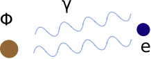
Figure 1: Charge ($e$) and fluxon ($\Phi$) in the vacuum. The mutual interaction between the two objects is mediated by the vacuum radiation field (represented by $\gamma$).

Quantum electrodynamic Hamiltonian of a charge and a fluxon-. The system considered comprises a charge $e$ and a ”fluxon” $\Phi$ in two spatial dimension (Fig. 1). This simplified configuration is sufficient to derive the essential physics of the AB effect. The interaction between the two entities is indirect, i.e., it is mediated by virtual photons (gauge field). The Hamiltonian of the system can be written as

$$H=\frac{1}{2m}(\mathbf{p}-\frac{e}{c}\mathbf{A})^{2}+\frac{\mathbf{P}^{2}}{2M}-\frac{\Phi}{4\pi}\hat{z}\cdot\mathbf{B}+\sum_{\mathbf{k},\lambda}\hbar\omega a_{\mathbf{k}\lambda}^{\dagger}a_{\mathbf{k}\lambda}\,,$$ (1)

where the motion of the particles is confined in the $x$-$y$ plane. The charge ($e$) with mass $m$ located at $\mathbf{x}_{a}$ interacts with the quantized radiation through the vector potential $\mathbf{A}$. In contrast, the fluxon ($\Phi$) with mass $M$ at $\mathbf{x}_{b}$ interacts with the magnetic field $\mathbf{B}$ of the radiation. The operator $a_{\mathbf{k}\lambda}^{\dagger}$ ($a_{\mathbf{k}\lambda}$) represents the creation (annihilation) of a photon with wave number $\mathbf{k}$ and polarization $\lambda$. Among the four possible modes of the polarization, only the two transverse modes are real excitation of radiation (last term of Eq. (1)).

The Hamiltonian can be rewritten as

$$H=H_{0}+V_{a}+V_{b},$$ (2a)

where

$$H_{0}=\frac{\mathbf{p}^{2}}{2m}+\frac{\mathbf{P}^{2}}{2M}+\sum_{\mathbf{k},\lambda}\hbar\omega a_{\mathbf{k}\lambda}^{\dagger}a_{\mathbf{k}\lambda}$$ (2b)

is the noninteracting part, and

$$V_{a}=-\frac{e}{mc}\mathbf{A}\cdot\mathbf{p}$$ (2c)

and

$$V_{b}=-\frac{\Phi}{4\pi}\hat{z}\cdot\mathbf{B}$$ (2d)

represent the charge–vacuum and fluxon–vacuum interactions, respectively. In the charge-potential interaction ($V_{a}$), we have omitted the term $(i\hbar/2mc)\nabla\cdot\mathbf{A}+(e^{2}/2mc^{2})\mathbf{A}^{2}$ which is independent of the charge variable and thus irrelevant to the present study.

We can observe the asymmetry between $V_{a}$ and $V_{b}$ in the role of the gauge field $\mathbf{A}$. The charge interacts with the radiation $\mathbf{A}$, which has some freedom of gauge selection. However, the interaction of the fluxon with the radiation is described by the gauge-independent $\mathbf{B}$. The gauge independence of $V_{b}$ can be confirmed by considering the fluxon as a current loop (with current $I$) interacting with $\mathbf{A}$ as

$$V_{b}=-\frac{I}{c}\oint\mathbf{A}\cdot d\mathbf{l}\,,$$ (3)

where the integration is made along the loop. Applying the Stokes’ theorem, we recover Eq.(2d), which is independent of gauge choice in $\mathbf{A}$.

The vector potential $\mathbf{A}$ corresponds to the spatial part of the four-potential $A^{\mu}$. The case of arbitrary gauge will be treated later. First, we begin with the Coulomb gauge ($\nabla\cdot\mathbf{A}=0$), where the two transverse modes (represented by $\lambda$) of $A^{\mu}$ are present:

$$\mathbf{A}(\mathbf{x},t)=\sum_{\mathbf{k},\lambda}\alpha_{\mathbf{k}}\left[u_{\mathbf{k}}(\mathbf{x})a_{\mathbf{k}\lambda}e^{-i\omega t}+u_{\mathbf{k}}^{*}(\mathbf{x})a_{\mathbf{k}\lambda}^{\dagger}e^{i\omega t}\right]\hat{e}_{\lambda}\,,$$ (4)

expanded by the plane wave modes $u_{\mathbf{k}}(\mathbf{x})=e^{i\mathbf{k}\cdot\mathbf{x}}/\sqrt{V}$ with normalization coefficient $\alpha_{\mathbf{k}}=\sqrt{2\pi\hbar c^{2}/\omega}$ and the corresponding angular velocity $\omega=ck$. The polarization $\hat{e}_{\lambda}$ is limited to the transverse modes by the constraint $\mathbf{k}\cdot\hat{e}_{\lambda}=0$ in the Coulomb gauge. The magnetic field of the radiation, given by $\mathbf{B}=\nabla\times\mathbf{A}$, is gauge-independent.

$$\mathbf{B}(\mathbf{x},t)=i\sum_{\mathbf{k},\lambda}k\alpha_{\mathbf{k}}\left[u_{\mathbf{k}}(\mathbf{x})a_{\mathbf{k}\lambda}e^{-i\omega t}-u_{\mathbf{k}}^{*}(\mathbf{x})a_{\mathbf{k}\lambda}^{\dagger}e^{i\omega t}\right]\hat{n}_{\lambda}\,,$$ (5)

where $\hat{n}_{\lambda}=\hat{\mathbf{k}}\times\hat{e}_{\lambda}$.

Canonical transformation and effective interaction-.
We adopt the canonical transformation technique to derive the charge–fluxon interaction mediated by the exchange of virtual photons. The Hamiltonian in (2) is transformed to $\tilde{H}=e^{-S}He^{S}$, where the first-order interaction part is eliminated by an appropriate choice of $S$. We obtain

$$\tilde{H} = H_{0}+H_{2}\,,$$ (6a)

$$H_{2} = \sum_{\gamma}|0\rangle\frac{\langle 0|V_{a}+V_{b}|\gamma\rangle\langle\gamma|V_{a}+V_{b}|0\rangle}{-\hbar\omega}\langle 0|\,,$$ (6b)

where $$|0\rangle |\gamma\rangle=a_{\mathbf{k}\lambda}^{\dagger}|0\rangle \langle 0|V_{a}|\gamma\rangle\langle\gamma|V_{a}|0\rangle \langle 0|V_{b}|\gamma\rangle\langle\gamma|V_{b}|0\rangle$$ denotes the radiation vacuum and . The self-interaction terms containing or are irrelevant and thus discarded. The second-order interaction between the two particles is given by

$$\tilde{H}_{2}=\sum_{\gamma}|0\rangle\frac{\langle 0|V_{a}|\gamma\rangle\langle\gamma|V_{b}|0\rangle+\mathrm{h.c.}}{-\hbar\omega}\langle 0|\,.$$ (6c)

The evaluation of the matrix elements in Eq. (6c) yields

$$\langle 0|V_{a}|\gamma\rangle = -\frac{e}{mc}\alpha_{\mathbf{k}}u_{\mathbf{k}}(\mathbf{x}_{a})(\hat{e}_{\lambda}\cdot\mathbf{p})e^{-i\omega t}\,,$$ (7a)

$$\langle\gamma|V_{b}|0\rangle = i\frac{\Phi}{4\pi}k\alpha_{\mathbf{k}}u_{\mathbf{k}}^{*}(\mathbf{x}_{b})(\hat{z}\cdot\hat{n}_{\lambda})e^{i\omega t}\,,$$ (7b)

and we obtain

$$\tilde{H}_{2}=\frac{ie\Phi}{2mc}F(\mathbf{x}_{a}-\mathbf{x}_{b})+\mathrm{h.c.}\,,$$ (8a)

where $$F$$ is a function of the relative position of the two objects given by

$$F(\mathbf{x})=\frac{1}{4\pi^{2}}\int d^{2}\mathbf{k}\frac{1}{k}e^{i\mathbf{k}\cdot\mathbf{x}}\sum_{\lambda}(\hat{e}_{\lambda}\cdot\mathbf{p})(\hat{z}\cdot\hat{n}_{\lambda})\,.$$ (8b)

Applying the condition $\hat{e}_{\lambda}\cdot\mathbf{k}=0$ in the Coulomb gauge, we find

$$(\hat{e}_{\lambda}\cdot\mathbf{p})(\hat{z}\cdot\hat{n}_{\lambda})=\hat{\phi}\cdot\mathbf{p}\,,$$

where $\hat{\phi}$ is the angular unit vector in the space of $\mathbf{k}$. Finally we can derive $\tilde{H}_{2}$ as

$$\tilde{H}_{2}=-\frac{e}{mc}\mathbf{p}\cdot\mathbf{a}\,,$$ (9a)

where the “effective vector potential” $$\mathbf{a}$$ is given by

$$\mathbf{a}(\mathbf{x})=\frac{\Phi}{2\pi|\mathbf{x}|}\hat{\theta}$$ (9b)

($\hat{\theta}$ denotes the azimuthal unit vector of $\mathbf{x}\equiv\mathbf{x}_{a}-\mathbf{x}_{b}$). This yields the expression of the effective Hamiltonian of Eq. (6)

$$\tilde{H}=\frac{1}{2m}\left(\mathbf{p}-\frac{e}{c}\mathbf{a}\right)^{2}\,,$$ (10)

where terms independent of the interaction between the the charge and the fluxon are omitted.

The expression of the “effective vector potential” in Eq. (9b) was previously obtained by adopting the QED approach Santos and Gonzalo (1999); Lee and Choi (2004), and it has recently been addressed in the context of the locality of the interaction Marletto and Vedral (2020); Saldanha (2021). Marletto and Vedral Marletto and Vedral (2020) and Saldanha Saldanha (2021) claimed that they had shown the locality of the interaction with particular selection of gauges (Coulomb and the Lorenz gauges, respectively). However, this claim is incomplete without an explicit derivation of the gauge invariance. This is clear if we compare it to the semiclassical approach where the vector potential $\mathbf{A}_{\Phi}$ produced by a magnetic flux possesses some degree of choosing the gauge with the constraint $\oint\mathbf{A}_{\Phi}\cdot d\mathbf{x}=\Phi$. The gauge invariance of $\mathbf{a}$ leads to a notable consequence in real experiments. Without the gauge invariant $\mathbf{a}$ we cannot predict the value of the local phase shift in a certain experimental arrangement Kang (2017), namely, the AB effect without an AB loop.

Gauge invariance of the interaction Hamiltonian and the local phase measurement-. Consider a gauge transformation of the four-potential $A^{\mu}\rightarrow A^{\prime\mu}=A^{\mu}+\partial^{\mu}\Lambda$ with an arbitrary single-valued scalar function $\Lambda=\Lambda(\mathbf{x},t)$. The vector potential $\mathbf{A}$ in Eq. (4) is then transformed to

$$\mathbf{A}^{\prime}=\mathbf{A}+\nabla\Lambda\,,$$ (11a)

where $$\Lambda$$ can be expanded as

$$\Lambda(\mathbf{x},t)=\sum_{\mathbf{k},\lambda}\left[\gamma_{\mathbf{k}}u_{\mathbf{k}}(\mathbf{x})a_{\mathbf{k}\lambda}e^{-i\omega t}+\gamma_{\mathbf{k}}^{*}u_{\mathbf{k}}^{*}(\mathbf{x})a_{\mathbf{k}\lambda}^{\dagger}e^{i\omega t}\right]\,,$$ (11b)

with an arbitrary $\mathbf{k}$-dependent coefficient $\gamma_{\mathbf{k}}$.

The additional contribution to $\tilde{H}_{2}$ of Eq. (6c) may be produced by $\partial^{\mu}\Lambda$ in the gauge transform. First, scalar potential $A^{0}$ is nonzero unlike in the Coulomb gauge. However, it does not couple to the motion of charge $\mathbf{p}$ and is irrelevant to the interaction between $q$ and $\Phi$. Second, the spatial part $\nabla\Lambda$ generates an additional term in $\tilde{H}_{2}$, given by

$$\delta\tilde{H}_{2}=\sum_{\gamma}|0\rangle\frac{\langle 0|\delta V_{a}|\gamma\rangle\langle\gamma|V_{b}|0\rangle+\mathrm{h.c.}}{E_{0}-E_{\gamma}}\langle 0|\,,$$ (12a)

where

$$\delta V_{a}=-\frac{e}{mc}\nabla\Lambda\cdot\mathbf{p}\,.$$ (12b)

$$\nabla\Lambda \mathbf{k}$$ consists of the longitudinal modes (parallel to ), and we obtain

$$\langle 0|\delta V_{a}|\gamma\rangle=-\frac{ie}{mc}k\gamma_{\mathbf{k}}u_{\mathbf{k}}(\mathbf{x}_{a})(\hat{\mathbf{k}}\cdot\mathbf{p})e^{-i\omega t}.$$ (12c)

However, this term does not couple to $\langle\gamma|V_{b}|0\rangle$, because the latter contains only transverse components (see Eq. (7b)). Therefore we conclude that $\delta\tilde{H}_{2}=0$. The second order interaction $\tilde{H}_{2}$ is gauge invariant.

This result of deriving gauge invariance in $\tilde{H}_{2}$ is remarkable. First, the gauge-invariant effective vector potential ($\mathbf{a}$ in Eq. (9b)) is in sharp contrast with the semiclassical counterpart. In the semiclassical approach, a charged particle under an external magnetic field is described by the Hamiltonian

$$H=\frac{1}{2m}\left(\mathbf{p}-\frac{e}{c}\mathbf{A}_{\Phi}\right)^{2}\,,$$ (13)

where the vector potential $\mathbf{A}_{\Phi}$, generated by $\Phi$, can be transformed to another function $\mathbf{A}_{\Phi}\rightarrow\mathbf{A}_{\Phi}+\nabla\chi(\mathbf{x})$. The constraint in $\mathbf{A}_{\Phi}$ is not local: $\oint\mathbf{A}_{\Phi}\cdot d\mathbf{r}=\Phi$.

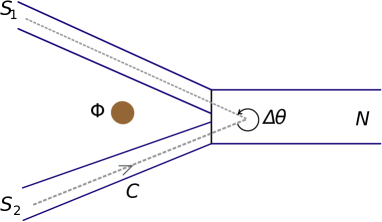
Figure 2: Schematic setup of the Andreev interferometer comprising two superconducting electrodes ($S_{1}$ and $S_{2}$) in contact with a normal metal ($N$).

Second, the gauge-invariant $\tilde{H}$ provides the unambiguous prediction of the local phase that can be measured in a certain type of experimental arrangement Kang (2017). The Hamiltonian (13) with semiclassical $\mathbf{A}_{\Phi}$ fails to make this prediction. Here, we briefly review the essential feature of the local phase measurement experiment (For the details, see Ref. Kang, 2017). Its schematic setup consists of two independent superconducting leads ($S_{1}$ and $S_{2}$), which are tunnel-coupled to a common normal electrode ($N$) (Fig. 2). The two superconducting electrodes are biased with identical voltages below the superconducting gap. The electrical current flows to the normal metallic output via Andreev reflection (AR) Andreev (1964), in which a Cooper pair is converted to two normal electrons in $N$. Interference is caused by the indistinguishability of the two different AR processes ($S_{1}$ to $N$ or $S_{2}$ to $N$), and the phase shift produced by the external flux is

$$\phi_{\mathrm{loc}}=\frac{e^{*}}{\hbar c}\int_{C}\mathbf{a}\cdot d\mathbf{x}=\frac{e^{*}\Phi}{2\pi\hbar c}\Delta\theta\,,$$ (14)

where the integration is considered along path $C$, as shown in Fig. 2. The effective charge $e^{*}=2e$ corresponds to the charge of a Cooper pair, and $\Delta\theta$ is the angle formed in the geometry of the system. The superconducting state is associated with gauge symmetry breaking, and the Cooper pairs satisfy the bosonic statistics. Therefore, the charge conservation and the Fermionic superselection rule do not prevent the interference in this setup (contrary to the argument in Ref. Marletto and Vedral, 2020).

Third, this value of the local phase (Eq. (14)) is equivalent to the result predicted by the semiclassical local field interaction (LFI) approach Kang (2017). As mentioned above, this cannot be achieved based on the semiclassical vector potential (Eq. (13)). With $\mathbf{A}_{\Phi}$, the local phase is given by $\phi_{\mathrm{loc}}=(e^{*}/\hbar c)\int_{C}\mathbf{A}_{\Phi}\cdot d\mathbf{x}$, and it is not invariant under the gauge transformation $\mathbf{A}_{\Phi}\rightarrow\mathbf{A}_{\Phi}+\nabla\chi$. This implies that the potential-based semiclassical approach fails to predict the value of $\phi_{\mathrm{loc}}$.

We need to address about how the ambiguity of the charge-flux interaction could be eliminated in the QED approach (represented by the effective vector potential $\mathbf{a}$ in Eq. (9b)). The key point is that the semiclassical Hamiltonian of Eq. (13) does not include the information regarding the local configuration of the system. Owing to the freedom of selecting a gauge in $\mathbf{A}_{\Phi}$, the same configuration of the flux can be described by a different function for $\mathbf{A}_{\Phi}$; furthermore, different locations of the flux may be expressed by the same $\mathbf{A}_{\Phi}$. In contrast, transformation of the gauge field (Eq. (11)) in the QED approach does not change the interaction Hamiltonian (Eq. (9a)). Its difference from the semiclassical vector potential is twofold. First, the local configuration of the charge and flux is well specified in the QED approach. Second, $\nabla\Lambda$ in the transformation of $\mathbf{A}$ (Eq. (11)) contains only the longitudinal modes in the gauge field. The longitudinal modes do not contribute to the interaction because the magnetic flux is coupled to the transverse modes.

It was recently proposed that the local phase $\phi_{\mathrm{loc}}$ can be predicted in the QED approach based on the particular choices of gauge Marletto and Vedral (2020); Saldanha (2021). As described above, this claim should be supported by an explicit demonstration of the gauge invariance of $\mathbf{a}$. This is evident if we compare it to the semiclassical vector potential $\mathbf{A}_{\Phi}$ in Eq. (13), where such a gauge invariance is not satisfied. We have explicitly shown the gauge invariance of the effective vector potential and confirmed that the QED approach eliminates the ambiguity in the interaction strength of the charge and flux.

Scalar photons and the scalar Aharonov–Bohm effect-. The gauge invariance of the effective vector potential $\mathbf{a}$ raises a question whether this invariance is universal for any type of the electromagnetic interaction mediated by virtual photons. In the following, we show that this is not the case if the scalar photons come into play. Consider a stationary charge ($e$) under external charge distribution ($\rho$) in the ideal force-free condition, as shown in Fig. 3. This condition can be achieved in real experiments Aharonov and Bohm (1959); Kim and Kang (2018), though it has never been realized. The generation of external potential with a vanishing electric field requires an appropriate distribution of charge density $\rho(\mathbf{x}^{\prime})$. In practice, this condition is achieved in the Faraday cage. The interaction between $e$ and $\rho$ is mediated by virtual photons, and the system is described by the Hamiltonian

$$H=H_{0}+eV(\mathbf{x},t)+\int\rho(\mathbf{x}^{\prime})V(\mathbf{x}^{\prime},t)\,,$$ (15a)

where $$H_{0} e \rho V A_{\mu}$$ represents the noninteracting part of , , and the electromagnetic vacuum, respectively. The charges interact with the scalar potential (time component of ) of the radiation

$$V(\mathbf{x},t)=A_{0}(\mathbf{x},t)=\sum_{\mathbf{k}}\alpha_{\mathbf{k}}\left[u_{\mathbf{k}}(\mathbf{x})a_{\mathbf{k}0}e^{-i\omega t}+u_{\mathbf{k}}^{*}(\mathbf{x})a_{\mathbf{k}0}^{\dagger}e^{i\omega t}\right]\,,$$ (15b)

where $a_{\mathbf{k}0}$ ($a_{\mathbf{k}0}^{\dagger}$) annihilates (creates) a photon in the scalar mode. Adopting the same canonical transformation technique used above (in obtaining Eq. (6)), we can derive the Coulomb interaction mediated by the virtual scalar photons (see e.g., Ref. Zee, 2010), as

$$\tilde{H}=H_{0}+e\int\frac{\rho(\mathbf{x}^{\prime})}{|\mathbf{x}-\mathbf{x}^{\prime}|}d^{3}\mathbf{x}^{\prime}\,.$$ (16)

This expression of the Coulomb interaction is derived from the exchange of virtual photons in the scalar mode. It is obtained by imposing the Lorenz gauge condition $\partial_{\mu}A^{\mu}=0$ and is not fully gauge-invariant. For instance, if we choose the Coulomb gauge, the scalar and longitudinal modes are absent. In this case, $V=0$ in Eq. (15b) and the Coulomb interaction of Eq. (16) cannot be derived.

This implies that the question regarding the reality of $A^{\mu}$ is more subtle in the quantum electrodynamics involving scalar modes. In any case, there are two notable points: The scalar photons (i) can never be observed but (ii) are indispensable as the mediator of the Coulomb interaction between two separate charges.

Conclusion-. In the quantum electrodynamic approach to the AB effect, the interaction between a charge and a magnetic flux is mediated by the exchange of virtual photons. We have shown the gauge invariance of the charge-flux interaction, which leads to an unambiguous prediction of the local phase shift. We have shown that the problem is more subtle in the electric AB effect. In contrast to the case of the magnetic AB, the scalar component of the gauge field plays an essential role and cannot be gauged away in the electric AB effect. This may indicate a significant role of the gauge field beyond mathematical construction.

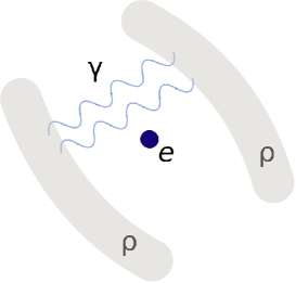
Figure 3: A charge ($e$) and the external charge distribution (represented by the charge density $\rho$). The scalar component of gauge field mediates the Coulomb interaction between $e$ and $\rho$.

References

- Ehrenberg and Siday (1949) W. Ehrenberg and R. Siday, Proceedings of the Physical Society. Section B 62, 8 (1949).
- Aharonov and Bohm (1959) Y. Aharonov and D. Bohm, Phys. Rev. 115, 485 (1959).
- Kang (2017) K. Kang, J. Kor. Phys. Soc. 71, 565 (2017).
- Kim and Kang (2018) Y.-W. Kim and K. Kang, New J. Phys. 20, 103046 (2018).
- Kang (2013) K. Kang, arXiv:1308.2093 (2013).
- Kang (2015) K. Kang, Phys. Rev. A 91, 052116 (2015).
- Marletto and Vedral (2020) C. Marletto and V. Vedral, Phys. Rev. Lett. 125, 040401 (2020).
- Saldanha (2021) P. L. Saldanha, Foundations of Physics 51, 1 (2021).
- Santos and Gonzalo (1999) E. Santos and I. Gonzalo, Europhysics Letters 45, 418 (1999).
- Lee and Choi (2004) M. Lee and M. Y. Choi, Journal of Physics A: Mathematical and General 37, 973 (2004); M. Y. Choi and M. Lee, Current Applied Physics 4, 267 (2004).
- Andreev (1964) A. Andreev, Sov. Phys. JETP 19, 1228 (1964).
- Zee (2010) A. Zee, Quantum field theory in a nutshell (Princeton university press, 2010).