Polarization and variability of compact sources measured in Planck time-ordered data

This paper introduces a new Planck Catalog of Polarized and Variable Compact Sources (PCCS-PV) comprising 153 sources, the majority of which are extragalactic. The data include both the total flux density and linear polarization measured by Planck  with frequency coverage from 30 to 353 GHz, and temporal spacing ranging from days to years. We classify most sources as beamed, extragalactic radio sources; the catalog also includes several radio galaxies, Seyfert galaxies, and Galactic and Magellanic Cloud sources, including H ii regions and planetary nebulae. An advanced extraction method applied directly to the multifrequency Planck time-ordered data, rather than the mission sky maps, was developed to allow an assessment of the variability of polarized sources. Our analysis of the time-ordered data from the Planck mission, tod2flux, allowed us to catalog the time-varying emission and polarization properties for these sources at the full range of polarized frequencies employed by Planck, 30 to 353 GHz. PCCS-PV provides the time- and frequency-dependent, polarized flux densities for all 153 sources. To illustrate some potential applications of the PCCS-PV, we conducted preliminary comparisons of our measurements of selected sources with published data from other astronomical instruments. In summary, we find general agreement between the Planck and the Institut de Radioastronomie Millimétrique (IRAM) polarization measurements as well as with the Metsähovi 37 GHz values at closely similar epochs. These combined measurements also show the value of PCCS-PV results and the PCCS2 catalog for filling in missing spectral (or temporal) coverage and helping to define the spectral energy distributions of extragalactic sources. In turn, these results provide useful clues as to the physical properties of the sources.

1 Introduction

There are many categories of prominent radio, millimeter-wave, and submillimeter sources, including Galactic sources such as H ii regions and supernovae remnants, and extragalactic systems such as quasars and dusty star-forming galaxies. The brightest of these sources at high frequencies, however, are typically either Galactic or active galactic nuclei (AGN). Both classes are considered here, though the bulk of our objects are extragalactic. AGN are the most powerful long-lasting sources in the Universe. Unlike much shorter timescale events such as black hole mergers or gamma-ray bursts, the active phase lasts long enough so that its properties and evolution can be studied in detail. Radio and submillimeter observations are central to understanding these systems. The radio emission of AGN is almost certainly related to a black hole at the center of the active galaxy and to the jets it engenders. These massive black holes in turn appear to be intimately related to the evolution of their host galaxies (Magorrian et al., 1998). AGN feedback in the form of radiation, winds, and relativistic jets is now invoked to explain the galaxy luminosity function and the $M$–$\sigma$ relation (e.g., Croton et al., 2006; Fabian, 2012; King & Pounds, 2015). The total power in the jets is a critical parameter in estimating the magnitude of this feedback. The physics required to estimate the jet power, however, is poorly understood. Important clues are provided by studies of both polarization and variability of emission from the jets. Such observations can illuminate the launching and initial propagation of relativistic jets, as well as the presence of jet “sheaths” and surrounding winds that could contribute to feedback (Blandford et al., 2019). The optical depth of the material surrounding the central black hole increases with wavelength, however. Hence millimeter and submillimeter observations are particularly useful: they allow us to study the properties of both the black hole and its surrounding accretion disk, as has been done for a few bright, relatively nearby, radio galaxies such as M87 (3C 274) (Junor et al., 1999; Hada et al., 2011) and 3C 84 (NGC 1275) (Giovannini et al., 2018). In these objects, as well as more distant radio galaxies and blazars, the millimeter–submillimeter continuum spectrum, time variability, and linear polarization probe the acceleration and collimation zone of the jet.

The observed properties of AGN strongly depend on the orientation between the line of sight and the axis of the jets.  Emission from the jet itself is dominant when the line of sight and jet axis align closely. This class of AGN, the blazars, includes BL Lac objects and flat-spectrum radio quasars (FSRQs). Doppler boosting causes the emission of the aligned jet to be strong and the counter-jet to be weak.  A substantial fraction of the AGN detected by Planck and other cosmic microwave background (CMB) experiments are blazars (Planck Collaboration XIII, 2011). That is not surprising, given the high apparent luminosity of blazars and their continuum spectra, which peak at millimeter to submillimeter wavelengths. The close alignment of jet and line of sight also allows for variability introduced by small changes in the angle between the line of sight and the jet (Begelman et al., 1984; Chen et al., 2013).

To maximize the science that can be extracted from radio and submillimeter observations of AGN, we ideally need high angular resolution, wide frequency coverage (extending to the submillimeter range) and repeated observations over time-scales of days to years including both total power and polarization measurements. Ground based interferometers, including the Atacama Large Millimeter Array (ALMA), meet the first of these needs. We show here that data derived as a byproduct of CMB experiments, properly analysed, can meet the last two. The sensitivity of current CMB experiments, including the Planck mission, is adequate to detect thousands of the brightest AGN. Most current CMB experiments now employ polarization-sensitive detectors and combine observations at several frequencies. Planck, for instance made polarized observations of the entire sky at seven frequencies from 30 to 353 GHz, some of them inaccessible from the ground. Finally, CMB searches generally cover large areas of the sky (the entire sky, in the case of Planck) repeatedly, providing observations of sources with cadences ranging from minutes to years.

To date, however, the potential contributions of CMB experiments and data sets have not been fully realized because the repeated observations of a given sky region are merely added together to produce static sky maps (Partridge et al., 2017). Combining repeated observations such as this makes perfect sense for the CMB and for Galactic foregrounds, both of which are static, but all information in the time domain is lost. We remedy that situation here by working with the time-ordered data (ToD) available from the multiyear Planck mission. The methods we employ can easily be extended to data coming from other CMB surveys. Here we provide a catalog of extragalactic sources measured in both total power and polarization by Planck, with frequency coverage from 30 to 353 GHz, and time-scales ranging from days to years.

We discuss the Planck mission, source selection, calibration and related topics in Sect. 2. In Sect. 3, we describe our technical approach to extracting flux density and polarization measurements from the Planck ToD, source by source and epoch by epoch. Sect. 4 describes the catalog we construct of these observations. Sect. 5 then treats the results and some consequences for models of AGN. We conclude in Sect. 6.

2 Planck data

All the data employed here were taken from archived time-ordered data (ToD) from the Planck mission as found in the Planck Legacy Archive. We first describe aspects of the mission relevant to our study, then describe how we selected bright sources. While most bright sources are AGN, we include some Galactic and thermal sources in our study. Galactic sources, such as the planetary nebula NGC 6572, are not expected to vary on short time scales, and hence provide a useful test of our pipeline.

2.1 The Planck mission

Planck was a European Space Agency (ESA) mission designed to map fluctuations in the CMB to the limit set by unavoidable cosmic variance down to angular scales of 5’ or so (Planck Collaboration I, 2020). Two instruments shared a common focal plane: the low-frequency instrument (LFI), with HEMT radiometers operating at 30, 44 and 70 GHz, and the high-frequency instrument employing lower-noise bolometric detectors in six frequency bands from 100 to 857 GHz. The fractional bandwidth at each frequency ranged from 20% to 30%. Polarization was measured at all but the two highest-frequency bands (545 and 857 GHz). Table 1 lists some of the relevant properties of the Planck mission. While mapping the CMB, Planck detected thousands of compact sources, both Galactic and extragalactic. Planck thus provides a valuable archive of observations of these sources, which we explore in this paper. These sources are cataloged, frequency by frequency, in several Planck catalogs; we employ only the latest, PCCS2 (Planck Collaboration XXVI, 2016). Approximate completeness limits in this catalog are provided in Table 1. These limits give a rough indication of the sensitivity of Planck to compact (unresolved) sources in each frequency band. A multifrequency catalog of Planck nonthermal sources is provided in Planck Collaboration Int. LIV (2018).

The scan strategy employed by Planck ensured that the full sky was covered twice in one year (Planck Collaboration I, 2014). Typically, a given source was observed at a given Planck frequency for a few days to one week in each six month survey (sources near the ecliptic poles, where Planck scans overlapped, were viewed much more frequently). HFI completed approximately five full sky surveys from 2009 August to 2012 January before its coolant ran out. LFI completed a fraction more than eight six-month surveys stretching from 2009 August to 2013 October. Thus we have five independent samples of flux densities at nine frequencies for each source, and an additional three or four measurements at 30, 44 and 70 GHz. The flux densities recorded in PCCS2 are averages over the entire mission, however, and thus smooth out any variability. In this paper, we work with the independent samples by analysing the time-ordered data (ToD).

Planck calibration at the frequencies employed here is determined from the satellite’s annual motion around the solar system barycenter (Planck Collaboration II 2020 for LFI; Planck Collaboration III 2020 for HFI). The calibration is thus absolute and precise to subpercent accuracy. This method of calibration has two consequences. First, the annual motion of the satellite produces a dipole signal in the CMB, much larger in angular scale than the beam width. In contrast the compact sources we investigate are almost never resolved, even at Planck’s highest frequency. Accurate calculations of flux density therefore require exact knowledge of the beam solid angle. The beam solid angles are known at each Planck band to percent-level accuracy (Planck Collaboration I, 2020). Second, the substantial bandwidth of the Planck detectors means that they respond differently to sources with spectra that differ from the blackbody spectrum of the CMB. Thus, for precision work, each measured flux density needs a small, spectrum-dependent, “color correction.” We return to this issue in Sect. 4 below.

Table 1: Relevant properties of the Planck instruments.

Band frequency	Center frequency	FWHM	Polarized?	90% completeness
(GHz)	(GHz)	(arcmin)		(mJy)
30   $\ldots$ $\ldots$ $\ldots$	028.3	32.29	yes	430
44   $\ldots$ $\ldots$ $\ldots$	044.0	27.94	yes	700
70   $\ldots$ $\ldots$ $\ldots$	070.2	13.08	yes	500
100   $\ldots$ $\ldots$ $\ldots$	100.3	09.66	yes	270
143   $\ldots$ $\ldots$ $\ldots$	141.6	07.22	yes	180
217   $\ldots$ $\ldots$ $\ldots$	219.6	04.90	yes	150
353   $\ldots$ $\ldots$ $\ldots$	359.0	04.92	yes	300
545   $\ldots$ $\ldots$ $\ldots$	555.4	04.67	no	550
857   $\ldots$ $\ldots$ $\ldots$	850.0	04.22	no	790

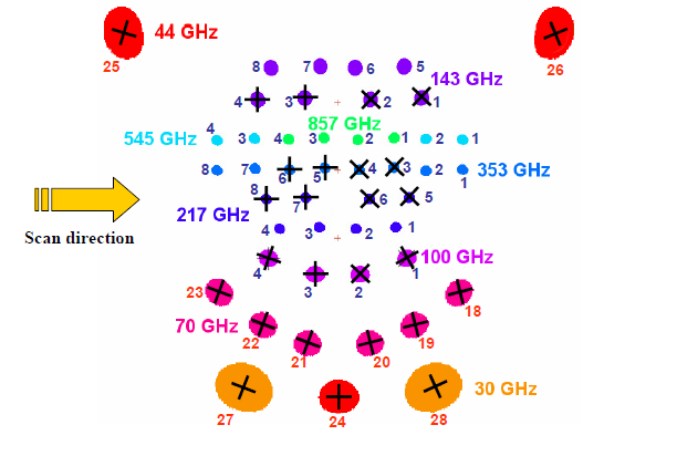
Figure 1: Footprint of the Planck focal plane as seen by an observer at infinity. The size of each colored spot is a rough indication of the relative resolution. The small crosses indicate polarization sensitivity.

2.2 Source selection

Given Planck’s relatively low sensitivity to compact sources and the low polarization fraction expected (a few percent; see, e.g., Datta et al. 2019), we elected to work only with the brightest sources in the Planck  PCCS2 catalog (Planck Collaboration XXVI, 2016). Specifically, we selected all PCCS2 sources with 100 GHz flux density greater than 1 Jy (roughly 15–20 times the $1\sigma$ uncertainty). Recall that the cataloged Planck flux densities are averages over the entire duration of the mission. Since most of these bright sources are variable, some may have fallen below the 1 Jy threshold for part of that period. The PCCS2 catalog yielded 148 sources above the 1 Jy threshold at 100 GHz; 111 were at Galactic latitude $>20^{\circ}$ and therefore likely to be extragalactic. This list included many well-known AGN such as 3C 454.3 and BL Lac. To this initial list, we added five sources well-studied in other high-frequency monitoring programs. In the end, we examined 153 sources, both Galactic and extragalactic. The majority were extragalactic, and most of these were blazars. The full list of sources with classification is shown in Table LABEL:tab:targets. Positions of all of the sources are indicated in Fig. 2.

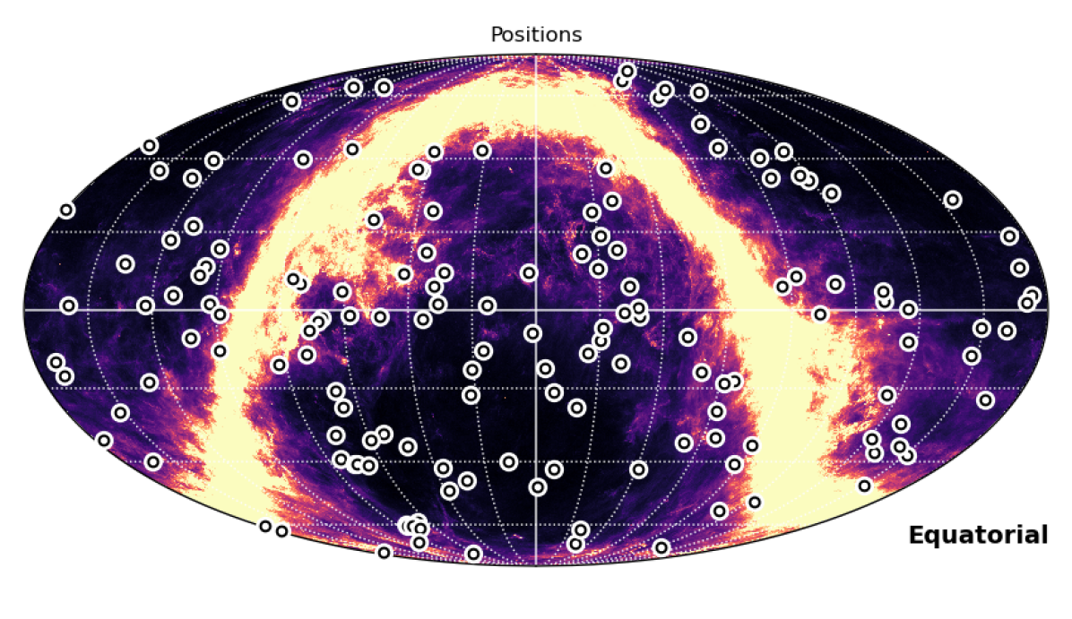
Figure 2: Positions of all 153 sources plotted over the Planck 857 GHz intensity map.

2.3 NPIPE processing

The Planck NPIPE data release (also known as PR4) differs from earlier data releases in several critical ways (Planck Collaboration Int. LVII, 2020). It is the first data release based on a single, stand-alone pipeline that processes both raw LFI and HFI data into calibrated, bandpass-corrected, noise-subtracted frequency maps. The release comprises frequency maps, Monte Carlo simulations, and calibrated timelines which we used as inputs to our processing. The timelines are accompanied by an updated instrument model that includes notable corrections to HFI polarization angles and efficiencies.

The NPIPE release is the first to include detector data acquired during so-called repointing maneuvers. Including these 4-minute periods between stable science scans not only increases integration time by about 9% but also improves sky sampling by adding detector samples between the regular scanning paths, which are separated by two arcminutes. NPIPE suppresses degree-scale noise in the maps by modeling the $1/f$ noise fluctuations in the data with $167\thinspace$ms noise offsets. In contrast, earlier LFI data were fitted with one-second offsets and earlier HFI data with full pointing period ($45$-minute) offsets.

We list here other systematic effects and artifacts corrected in NPIPE processing:

• electrical interference from housekeeping electronics (for LFI) and the 4-kelvin cooler (for HFI);

• jumps in signal offset;

• cosmic ray glitches (HFI);

• bolometric nonlinearity (HFI);

• thermal common modes (HFI);

• ADC nonlinearity (HFI);

• gain fluctuations;

• bandpass mismatch from both continuum emission and CO lines;

• bolometric transfer function and transfer function residuals (HFI);

• far-sidelobe pickup.

In addition, NPIPE removes time-dependent signals from the orbital dipole and Zodiacal light that would otherwise compromise mapmaking.

3 Technical approach

As noted above, Planck sees most compact sources on the sky only once during each six-month sky survey. We call the roughly week-long period during which the Planck detectors collect time samples in the vicinity of a source an observation. During each observation, the orientation of the detectors with respect to the source remains fixed. Consequently, individual detectors cannot resolve the polarized flux density from the intensity in a single observation. To overcome this restriction, different detectors in a given Planck band are given different polarization angles (see Fig. 1).

3.1 Individual detectors

To solve for the polarized flux density, we first measured the polarization-modulated flux density seen by each of the Planck detectors. The data model can be cast in the typical linear regression form:

$$\@vec{d}=F\@vec{a}+\@vec{n},$$ (1)

where

• $\@vec{d}$ is the vector of detector samples that fall within some fitting radius from the source coordinates;

• $F$ contains the time-domain templates representing the source and the background. The primary template in $F$ is the detector point spread function (PSF). This is the beam pattern produced when a detector with finite resolution scans a point source.

• $\@vec{a}$ contains the template amplitudes;

• $\@vec{n}$ is the detector noise.

The maximum likelihood solution for the template amplitudes, $\@vec{a}$, is:

$$\@vec{a}=\left(F^{\mathrm{T}}N^{-1}F\right)^{-1}F^{\mathrm{T}}N^{-1}\@vec{d},$$ (2)

where $N$ is the noise covariance matrix $N=\langle\@vec{n}\@vec{n}^{\mathrm{T}}\rangle$. The Planck PR4 timelines used as inputs are calibrated and destriped, making a diagonal noise matrix, $N=\sigma^{2}\mathbf{1}$, an excellent approximation. Furthermore, the detector samples in $\@vec{d}$ are separated in time by 60 s, the time it takes for Planck to spin around, effectively breaking sample-sample noise correlations.

The PSF must be rotated into the appropriate orientation and centered at the cataloged source position. The fitted amplitude of the PSF template is readily translated into a flux density across the detector pass band. Since the detector data are calibrated in thermodynamic units, the fitted amplitudes must be translated into flux density using the unit conversion factors derived from ground-measured band-passes. The full unit conversion is

$$f=T_{\mathrm{max}}\thinspace\Omega_{\mathrm{det}}\thinspace u_{\mathrm{det}},$$ (3)

where $T_{\mathrm{max}}$ is the peak temperature read off the PSF fit, $\Omega_{\mathrm{det}}$ is the solid angle of the PSF and $u_{\mathrm{det}}$ is the unit conversion factor from kelvin to MJy/sr, derived by convolving the detector bandpass with a standard source spectrum (slope $\alpha=-1$).

Additional columns in $F$ model the background [foreground] emission. There is always a constant offset template, but we also considered higher-order templates such as slopes. Keeping the fitting radius close to the beamwidth limits the number of modes needed to fully model the background [foreground].

Small offset between the catalog source position and apparent source location can be modeled by adding spatial derivatives of the PSF in $F$. Such offsets naturally rise if the source position was originally fitted over a pixelized sky map. There can also be small pointing errors in the Planck data themselves. Finally, the center of the PSF template is slightly arbitrary and can be defined as either the peak or the center of weight. For vast majority of our targets, including position corrections in the fit increases uncertainty without a significant improvement in the quality of the fit. The few cases where the improvement is statistically significant (source is very bright), the change in measured flux density is less than a percent. Therefore the reported flux densities are based on fits directly at the catalog positions.

3.2 Polarized flux density

For a given observation, each detector produces one data point: the polarization-modulated flux density:

$$f_{d}=I+\eta_{d}\left[Q\cos(2(\psi+\psi_{d}))+U\sin(2(\psi+\psi_{d}))\right],$$ (4)

where

• $f_{d}$ is the polarization-modulated flux density measured with detector $d$;

• $I$, $Q$ and $U$ are the Stokes parameters of the source flux density (CMB detectors are not typically sensitive to $V$, the circular polarization component);

• $\eta$ is the detector polarization efficiency – an ideal polarization-sensitive detector would have $\eta=1$;

• $\psi$ represents the angle between the source coordinate system and the focal-plane coordinate system;

• $\psi_{d}$ is the polarization sensitive direction of the detector in the focal-plane coordinates.

A vector of detector fluxes, $\@vec{f}$, can be modeled as

$$\@vec{f}=P\@vec{m}+\@vec{n},$$ (5)

where each row of the pointing matrix, $P$, comprises the pointing weights, $[1,\eta\cos(2(\psi+\psi_{d})),\eta\sin(2(\psi+\psi_{d}))]$, for one detector, and the “map” vector contains the three Stokes parameters: $m=[I,Q,U]^{\mathrm{T}}$. The noise vector, $n$, contains the measurement uncertainty for each detector. Analogous to Eq. (2), the maximum likelihood solution reads:

$$\@vec{m}=\left(P^{\mathrm{T}}N^{-1}P\right)^{-1}P^{\mathrm{T}}N^{-1}\@vec{f}.$$ (6)

The theory of linear regression also provides the covariances:

$$N_{m}=\langle\Delta\@vec{m}\Delta\@vec{m}^{\mathrm{T}}\rangle=\left(P^{\mathrm{T}}N^{-1}P\right)^{-1}=\begin{bmatrix}\sigma_{I}^{2}&\sigma_{IQ}&\sigma_{IU}\\ &\sigma_{Q}^{2}&\sigma_{QU}\\ &&\sigma_{U}^{2}\end{bmatrix},$$ (7)

where we have omitted the redundant elements in the symmetric covariance matrix.

In order to derive the polarization fraction and polarization angle, we defined two estimators:

$$\hat{p}=\frac{\sqrt{Q^{2}+U^{2}}}{I}\quad\mathrm{and}\quad\hat{\psi}=\frac{1}{2}\arctan{\frac{U}{Q}}.$$ (8)

While these estimators are textbook definitions of the polarization parameters, they are biased by uncertainties in $I$, $Q$, and $U$. Finding unbiased or minimally biased estimators for these parameters turns out to be complicated and depends on the signal-to-noise ratio (S/N) of the $I,Q,U$ estimates. For the modest S/N in our case, we have adopted the asymptotic estimator from Montier et al. (2015):

$$\hat{p}_{\mathrm{AS}}=\cases{\sqrt{\hfil}}{\hat{p}^{2}-b^{2}}&\mathrm{if}\thinspace\thinspace\hat{p}>b,\\ 0\mathrm{otherwise}{},$$ (9)

where

$$b^{2} = \frac{\widetilde{\sigma}_{U}^{2}\cos^{2}\left(2\psi_{0}-\theta\right)+\widetilde{\sigma}_{Q}^{2}\sin^{2}\left(2\psi_{0}-\theta\right)}{I_{0}^{2}}$$ (10)

$$\theta = \frac{1}{2}\arctan\left(\frac{2\rho\sigma_{Q}\sigma_{U}}{\sigma_{Q}^{2}-\sigma_{U}^{2}}\right)$$ (11)

$$\widetilde{\sigma}_{Q}^{2} = \sigma_{Q}^{2}\cos^{2}\theta+\sigma_{U}^{2}\sin^{2}\theta+\rho\sigma_{Q}\sigma_{U}\sin 2\theta$$ (12)

$$\widetilde{\sigma}_{U}^{2} = \sigma_{Q}^{2}\sin^{2}\theta+\sigma_{U}^{2}\cos^{2}\theta-\rho\sigma_{Q}\sigma_{U}\sin 2\theta$$ (13)

$$\rho = \frac{\sigma_{QU}}{\sigma_{Q}\sigma_{U}}.$$ (14)

The estimator from Eq. (8) is typically substituted in place of the true polarization angle, $\psi_{0}$.

Confidence regions for the polarization parameters are determined using a Monte Carlo method: we sampled 100,000 triplets of true $(I_{0},p_{0},\psi_{0})$ and recorded the likelihood of the measured $(I,p,\psi)$. From those likelihoods, we inferred the 68% and 95% confidence regions for the true polarization parameters. The Bayesian likelihood, $\mathcal{L}(I,p,\psi|I_{0},p_{0},\psi_{0})$, is defined in Montier et al. (2015), Eqs. (3) and (23). Examples of the sampled likelihood, projected to the $p$-axis are shown in Fig. 3.

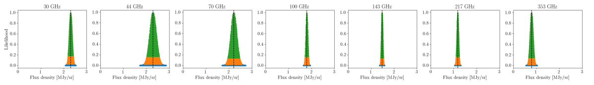
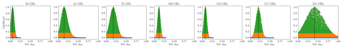
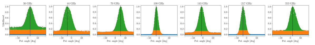
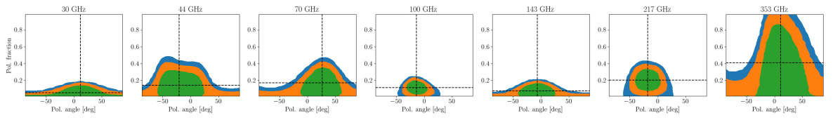
Figure 3: 100,000 sampled values of the likelihood function, projected to the intensity axis (top row), polarization fraction axis (2nd row) or polarization angle axis (3rd row). The source, PCCS2 143 G052.40$-$36.49 also known as 4C $-$02.81, was chosen because it has both positive detections of and upper limits on polarization fraction. The likelihood threshold that includes 68 % of the total likelihood is indicated in green and 95 % in orange. Samples with likelihood lower than 95 % of the distribution are in blue. When the green part of the polarization fraction distribution excludes zero, we report a 68 % confidence interval. When zero is included, we report a 95 % upper limit. The bottom row presents the maximum of the likelihood function in the polarization fraction-polarization angle plane. The dashed lines indicate the maximum likelihood values. The likelihoods are based on the first survey shown in Fig. 4.

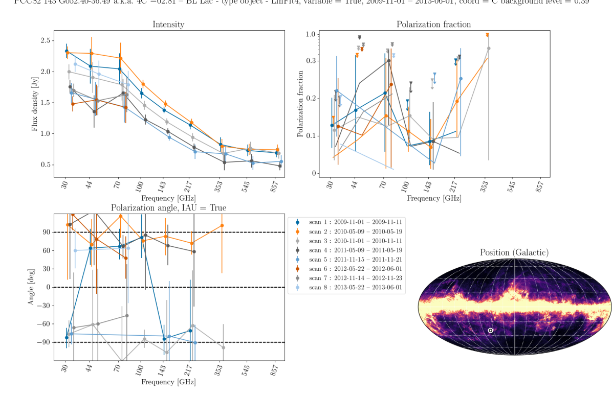
Figure 4: Example of a full diagnostic plot showing intensity, polarization fraction, polarization angle, and position for PCCS2 143 G052.40-36.49. The polarization fraction axis is nonlinear between $0.3$ and $1.0$ to accommodate all values. The lines and points of different colours mark different observing epochs, separated by 6 months. The Galactic-coordinate map (HEALPix formatted, Górski et al. 2005) in the lower right panel shows the position of the source on top of the Planck 857 GHz intensity map. Plots and maps similar to this are provided for each source and each number of jointly fit frequencies.

3.3 Multifrequency fits

In addition to tabulating flux densities at each Planck frequency, we provide multifrequency fits in order to improve the S/N of the measured polarized flux densities. A fit such as this necessarily requires some accommodation of the source spectral energy distribution (SED). We extended the signal model in Eq. (4) to:

$$f_{d}=\left(\frac{\nu_{d}}{\nu_{0}}\right)^{\alpha}\Big{\{}I+\eta_{d}\left[Q\cos(2(\psi+\psi_{d}))+U\sin(2(\psi+\psi_{d}))\right]\Big{\}},$$ (15)

where $\alpha$ is the spectral index of the source, $\nu_{d}$ is the central frequency of detector $d$, and $\nu_{0}$ is the noise-weighted central frequency of all detectors that are being combined. This model implies strong constraints on the fit:

• the SED is approximated as a power-law across the fitted frequencies;

• the spectral indices of intensity and polarized emission are the same;

• the polarization fraction and angle do not depend on the frequency.

These approximations obviously break down as increasingly wider frequency ranges are considered. Hence we provide multi-frequency fits only up to three adjacent frequency bands. Within these bands, and to the extent the approximations are valid, the additional constraints greatly improve the S/N of our fits.

3.4 Software

Our flux-fitting software is implemented in Python-3 and released as open source software. The package includes Planck-specific specializations but they are modularized and the software can be adapted for other experimental data sets that can be sampled into the small data set format used as inputs to the calculation.

4 The catalog

Our catalog of time- and frequency-dependent, polarized, flux densities is spread over multiple comma-separated value (CSV) files. Each file features a single source and the entries correspond to a fixed number (ranging from 1 to 3) of frequency bands averaged together. The filenames are of the form results_<PCCSNAME>_nfreq=<NFREQ>.csv, where <PCCSNAME> is the name of the source in the 143 GHz Planck PCCS2 catalog and <NFREQ> is the number of frequency bands averaged for each entry (1, 2, or 3). The fields of the files are

1. band(s) – nominal Planck bands comprising the entry.

2. freq [GHz] – noise-weighted average of the nominal frequencies.

3. start – approximate UT calendar date of the start of the observations used in deriving the entry.

4. stop – approximate UT calendar date of the end of the observations.

5. I flux [mJy] – intensity flux density at the effective central frequency, not color-corrected to match freq [GHz].

6. I error [mJy] – 1-$\sigma$ uncertainty of the I flux [mJy]

7. Q flux [mJy] – linear $Q$-polarization flux density in IAU convention and Equatorial (J2000) coordinates.

8. Q error [mJy] – 1-$\sigma$ uncertainty of Q flux [mJy].

9. U flux [mJy] – linear $U$-polarization flux density in IAU convention and Equatorial (J2000) coordinates.

10. U error [mJy] – 1-$\sigma$ uncertainty of U flux [mJy].

11. Pol.Frac – debiased polarization fraction in the range [$0\ldots 1$].

12. PF low lim – Bayesian 16% quantile lower limit of Pol.Frac or zero.

13. PF high lim – If PF low lim is nonzero the Bayesian 16% quantile upper limit of Pol.Frac. Otherwise the 95% upper limit.

14. Pol.Ang [deg] – Polarization angle in IAU convention and Equatorial (J2000) coordinates.

15. PA low lim – Bayesian 16% quantile lower limit of Pol.Ang [deg].

16. PA high lim – Bayesian 16% quantile upper limit of Pol.Ang [deg].

An excerpt of one catalog file is shown in Appendix A. The CSV file is accompanied by two diagnostic plots that visualize its contents:

• flux_fit_<PCCSNAME>_nfreq=<NFREQ>.png

• results_<PCCSNAME>_nfreq=<NFREQ>.replot.png

The first of these shows the fit data as a function of frequency (e.g., Fig. 4) and the second as a function of time (e.g., Fig. 5).

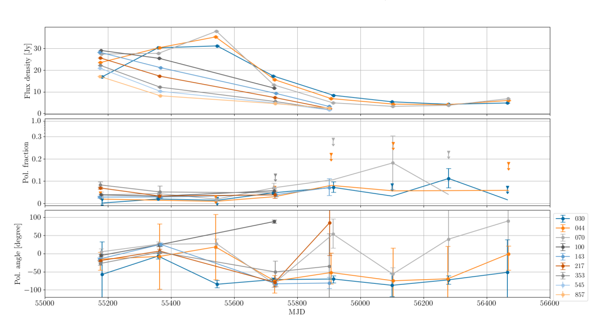
Figure 5: Time-series plot of our flux density fits to 3C 454.3 observations. The HFI data for the third pass are missing due to quality flagging.

For convenience, we also provide a single catalog file, combined.csv, that combines entries from all individual results_*csv files so that it includes data for all 153 sources. This file has three additional columns appended to the beginning of each row:

• target – Name of the target in the Planck 143GHz PCCS2 catalog;

• RA – Right ascension in degrees (J2000);

• Dec – Declination in degrees (J2000).

The flux densities in our catalog are not color-corrected. That is, we made no effort to translate the measured flux density to the nominal observing frequency. The reason is that the spectral indices of the sources can vary as a function of time and across the Planck pass-band, and the small corrections (of order a few percent) depend on a source’s spectral index. Instead, we present in Table 2 the effective central frequencies of the Planck bands for a number of spectral slopes. The formulas for evaluating the central frequency are laid out in Planck Collaboration IX (2014).

Our catalog, PCCS-PV, will be available at the ESA Planck Legacy Archive. and at the NASA/IPAC Infrared Science Archive.

Table 2: Effective central frequency in GHz as a function of the nominal frequency and spectral index across the pass-band.

Nominal frequency		Spectral index $\alpha$
(GHz)		$-2$	$-1$	$0$	$1$	$2$	$3$	$4$
30	$\ldots$ $\ldots$ $\ldots$	28.10	28.28	28.46	28.64	28.83	29.03	29.22
44	$\ldots$ $\ldots$ $\ldots$	43.79	43.94	44.09	44.25	44.40	44.55	44.69
70	$\ldots$ $\ldots$ $\ldots$	69.43	69.90	70.36	70.80	71.24	71.66	72.07
100	$\ldots$ $\ldots$ $\ldots$	99.36	100.28	101.23	102.22	103.28	104.46	105.95
143	$\ldots$ $\ldots$ $\ldots$	139.82	141.17	142.57	144.04	145.59	147.28	149.18
143	P   $\ldots$ $\ldots$ $\ldots$	139.29	140.63	142.04	143.52	145.10	146.83	148.77
217	$\ldots$ $\ldots$ $\ldots$	218.08	220.03	222.02	224.05	226.14	228.30	230.60
217	P   $\ldots$ $\ldots$ $\ldots$	217.18	219.18	221.23	223.32	225.47	227.69	230.04
353	$\ldots$ $\ldots$ $\ldots$	355.38	358.07	360.82	363.62	366.47	369.40	372.44
353	P   $\ldots$ $\ldots$ $\ldots$	354.57	357.22	359.93	362.70	365.53	368.45	371.50
545	$\ldots$ $\ldots$ $\ldots$	547.42	552.80	558.00	563.01	567.84	572.45	576.83
857	$\ldots$ $\ldots$ $\ldots$	845.64	853.99	862.02	869.76	877.23	884.40	891.26

5 Results and discussion

5.1 Polarized signal-to-noise ratio

The targets in our catalog vary in intensity, polarization fraction and spectral properties. We explore the polarized S/N of our catalog in Fig. 6. The Figure shows the scatter in polarized S/N as a function of the intensity flux density and identifies a threshold beyond which half of the observations reach S/N of one. The threshold varies considerably across the Planck frequencies and obviously depends on the spectral and polarization properties of our catalog.

Our most sensitive, single frequency measurements of polarized flux density come from the 143 GHz band where the S/N is higher than unity in a majority of observations when the source is brighter than 1.86 Jy. Fitting for the source spectral index and combining frequencies gives us a combined threshold better than 1.5 Jy in all frequency combinations involving 143 GHz. Combining the Planck LFI frequencies (30–70 GHz) has a combined threshold of 2.20 Jy.

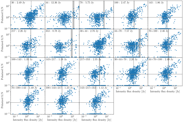
Figure 6: Polarized S/N: for each polarization-sensitive observation in our catalog, we plot the de-biased polarized flux density S/N against the intensity flux density. Observing bands are indicated in the labels. For cases where de-biasing renders a S/N less than 0.1, we plot a data point at 0.1. The vertical grey bands indicate the lowest and narrowest flux density bin that has a median S/N of 1.0 and at least 20 entries. The center of the bin is spelled out in the label.

5.2 Characterization

We made use of both spectral information and classifications from the literature, mainly NED (Helou et al., 1995) and SIMBAD (Wenger et al., 2000), to divide our sample of 153 sources into several categories. The majority are extragalactic, but nine (6%) are Galactic sources such as H ii regions or planetary nebulae, and five more are H ii regions located in the Magellanic Clouds. Many of the extragalactic objects are well-studied radio sources such as 3C 84 or M87. We characterize the 139 extragalactic sources as $\sim$25% BL Lac objects, $\sim$60% quasars and $\sim$10% Seyfert-1 galaxies. Some sources exhibit both synchrotron emission with a falling spectrum and dust emission at the highest Planck frequencies (see Fig. 8 for an example).

The few Galactic (and LMC) sources are not beamed and have large physical dimensions, so they are unlikely to be variable on time scales of a few years or less. They therefore offer an opportunity to check the fidelity of our pipeline. Fig. 7 provides an example. PCCS2 143 G000.35$-$19.48 is a Galactic dark cloud, and, as expected, shows no statistically significant variation with epoch at any Planck frequency except for some scatter at 44 GHz, which has the highest noise among the Planck bands. In addition, as shown in Fig. 1, the three 44 GHz beams lie at the periphery of the Planck field of view, and two of the beams have much higher ellipticity than the other one. Consequently, the measured flux density at that frequency depends on how the source crosses the focal plane, and hence may show some instrument-related variation.

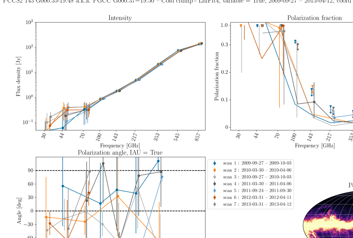
Figure 7: SED of a Galactic source, PCCS2 143 G000.35$-$19.48 at RA = $287.56^{\circ}$ and dec = $-37.15^{\circ}$. The lines and points of different colors mark different observing epochs, separated by 6 months. It is important to note the larger scatter of the noisier LFI measurements at 30, 44, and 70 GHz. With the possible exception of 44 GHz, there is no evidence for variability, as expected for a large source of this type.

Some extragalactic sources also demonstrate no significant variation during the Planck mission. We show two examples in Fig. 8. G021.20+19.62 (3C 353) is an radio galaxy with a spectral upturn at 545 GHz showing no variation in flux density at any frequency. The polarization percentage, while small, also does not appear to vary.

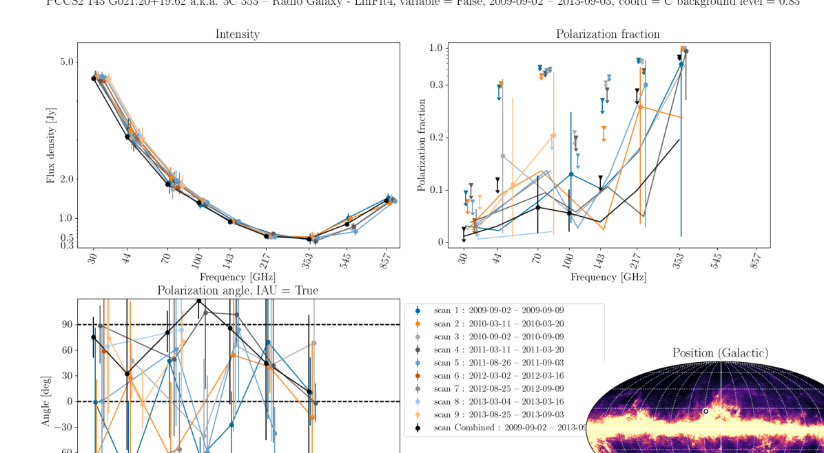
Figure 8: Same as in Fig. 7, but the lines and points of different colors mark different observing epochs, separated by 6 months. For the polarization fraction (right column) we plot the maximum likelihood value as a solid line and indicate a 68% confidence region or 95% upper limit with error bars. Top: An AGN (3C 353) displaying no significant changes in SED, and small, but apparently constant polarization. Bottom: A BL Lac object, PKS 1514$-$24, showing only mild variability, and no significant change in polarization.

Of more interest are those sources that clearly do vary during the Planck mission. The blazar PCCS2 143 G086.11$-$38.19 (3C 454.3), for instance, is a well-known and well-studied variable source that is known to have flared during the Planck mission (Planck Collaboration XIV, 2011). We discuss 3C 454.3 in some detail below (see Fig. 5).

In Fig. 9, we show the SED of another strongly variable source, G304.15$-$72.18 at RA = $12.32^{\circ}$, dec = $-44.95^{\circ}$. There is clear evidence of spectral change with epoch. Strong variability is also evident in the following sources, among others: G106.95$-$50.62 (a Seyfert-1 galaxy), G315.80$-$36.52 (a QSO), and G352.45$-$08.41 (a blazar).

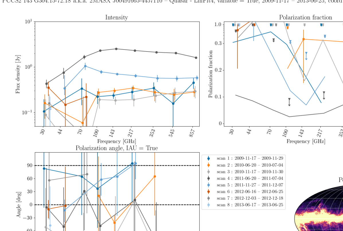
Figure 9: Strongly variable source, PCCS2 143 G304.15$-$72.18. It is apparent that the spectral shape, as well as luminosity, changes with epoch.

5.3 Concurrent observations with other instruments

In order to check our measurements and to illustrate possible uses of the data presented here, we compare the Planck polarization data of selected objects with published data from other astronomical instruments. Fig. 10 presents the Planck data of the BL Lac object OJ 287 alongside the 37 GHz light curve from the Metsähovi Radio Observatory (as summarized in Planck Collaboration Int. XLV 2016), linear polarization at 86 and 230 GHz measured with the 30-meter antenna of the Institut de Radioastronomie Millimétrique (IRAM, Agudo et al., 2018), and Very Long Baseline Array (VLBA) images that include linear polarization (Jorstad et al., 2017). Fig. 11 provides a similar plot for the quasar 3C 454.3. For comparison, we present in Figures 12 and 13 VLBA images at 43 GHz of OJ 287 and 3C 454.3 obtained within one month of an epoch for which we have Planck polarization measurements. The images are from the VLBA–BU Blazar Monitoring Program. We find that the flux densities at 30 and 44 GHz agree with the Metsähovi 37 GHz values at nearby epochs. In addition, there is general correspondence between the Planck and IRAM polarization. These similarities serve to validate our measurements.

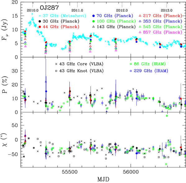
Figure 10: Flux density and polarization versus time of the BL Lac object OJ 287. Frequencies and sources of the data are indicated in the figure. The figure does not plot the following upper limits: 44 GHz: MJD 55301–55309 ($\leq 34\%$), 55497–55505 ($\leq 30\%$), 55666–55674 ($\leq 24\%$), 56038–56050 ($\leq 27\%$), 56236–56247 ($\leq 42\%$); 70 GHz: MJD 56238–56241 ($\leq 31\%$), 56410–56413 ($\leq 31.2\%$); 353 GHz: MJD 55304–55305 ($\leq 77\%$), 55500–55501 ($\leq 52\%$), 55669–55670 ($\leq 37\%$). No polarization was detected at 545 or 857 GHz, since the HFI detectors are unpolarized at those frequencies.

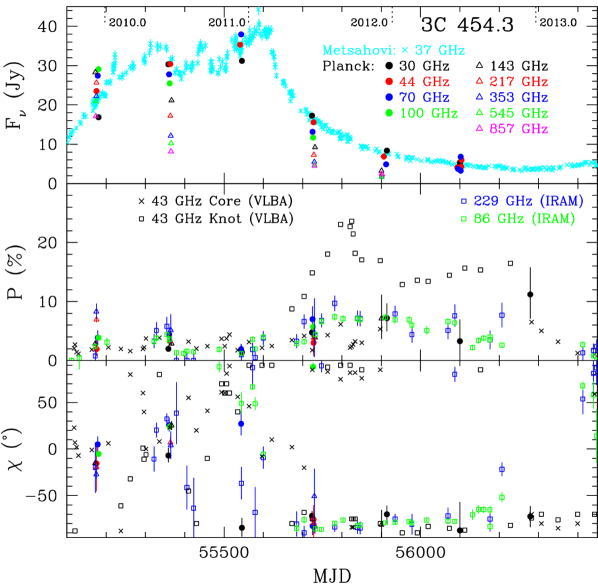
Figure 11: Flux density and polarization versus time of the quasar 3C 454.3. Frequencies and sources of the data are indicated in the figure. The figure does not plot the following upper limits: 30 GHz: MJD 55179–55182 ($\leq 2.4\%$), 56464–56465 ($\leq 11\%$); 44 GHz: MJD 55357–55369 ($\leq 3.6\%$), 55535–55546 ($\leq 4.6\%$), 55899–55914 ($\leq 36\%$), 56089–56097 ($\leq 42\%$), 56277–56285 ($\leq 41\%$), 56464–56472 ($\leq 29\%$); 70 GHz: MJD 55912–55913 ($\leq 47\%$), 56101–56103 ($\leq 64\%$), 56277–56279 ($\leq 36\%$), 56465–56467 ($\leq 18\%$); 217 GHz: MJD 55902–55902 ($\leq 27\%$); 353 GHz: MJD 55901–55901 ($\leq 100\%$). No polarization was detected at 545 and 857 GHz.

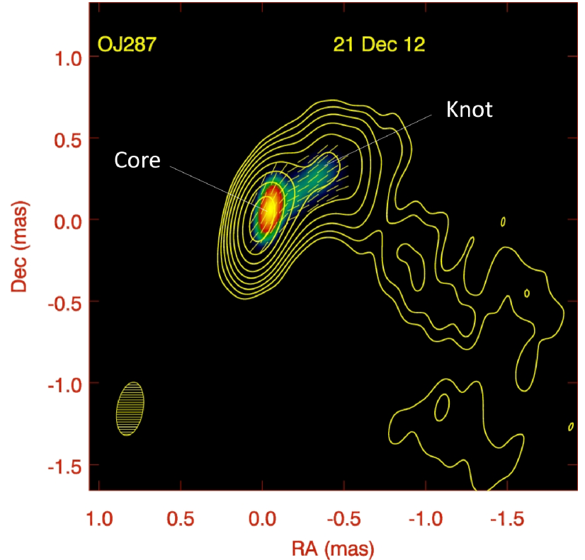
Figure 12: VLBA image of OJ 287 at 43 GHz at epoch 2012 December 21 (MJD 56282). The contours represent total intensity, starting at 0.25% of the maximum of 0.79 Jy/beam and increasing by factors of 2. The color scale represents linearly polarized intensity, with maximum value (yellow) of 0.032 Jy/beam. The yellow line segments indicate the EVPA. The restoring beam FWHM, representing the angular resolution, is displayed in the lower left corner.

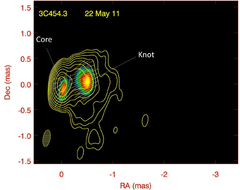
Figure 13: VLBA image of 3C 454.3 at 43 GHz at epoch 2011 May 22 (MJD 55704). The contours represent total intensity, starting at 0.25% of the maximum of 6.00 Jy/beam and increasing by factors of 2. The color scale represents linearly polarized intensity, with maximum value (yellow) of 0.27 Jy/beam. The yellow line segments indicate the EVPA. The restoring beam FWHM, representing the angular resolution, is displayed in the lower left corner.

Figure 14: Frequency dependence of the flux density, degree of linear polarization, and EVPA of 3C 454.3 in 2009 December. For frequencies $\leq 353$ GHz, the data are from this work. The high-frequency point is at optical R band from Jorstad et al. (2013).

Figure 10 demonstrates that the Planck polarization of OJ 287 is similar to that of the core seen in Fig. 13. We note that the optical electric-vector position angle (EVPA) of the knot deviates at some epochs from the source-integrated polarization at 30–353 GHz. Sasada et al. (2018) have shown that the optical polarization is related to that of either the core or the knot, depending on the epoch. Our data are consistent with this conclusion.

Figure 14 presents the frequency dependence of the flux density, degree of polarization, and EVPA of 3C 454.3 during the first Planck survey in late 2009. At that epoch, an extremely high-amplitude two-year outburst was in its early, rising stage. The core completely dominated the polarization in a VLBA image obtained 17 days earlier (from the VLBA-BU-BLAZAR website). Figure 14 reveals that the degree of polarization was higher by a factor of $\sim 2$ from 44–100 GHz below the spectral turnover than at 217–353 GHz above the turnover. There is a frequency gradient in EVPA from $\sim 5^{\circ}$ to $\sim-30^{\circ}$ from 70 to 353 GHz. At the same epoch, the optical R-band EVPA was $-37^{\circ}\pm 2.1^{\circ}$, having shifted from $+25^{\circ}$ nine days earlier (Jorstad et al., 2013). The degree of polarization at R band was $15.4\pm 1.8\%$. This frequency dependence strongly implies that the outburst involved a component that dominated the emission from $\sim 200$ GHz to optical frequencies. We are therefore able to conclude that the optical flare occurred within the same region as the $\sim 200$ GHz flare, which is distinct from the regions (probably farther downstream in the jet) that dominate the emission at lower frequencies.

5.4 Planck’s contribution to the overall spectral energy distribution

In Figures 15 and 16 we present the Planck data from PCCS2 (Planck Collaboration XXVI, 2016). For the remaining three sources, Centaurus A, 3C 84, and Pictor A, the Planck data help to fill in some missing spectral coverage. In particular, in Centaurus A, the Planck data help to define the rise into the spectral region dominated by the infrared dust component.

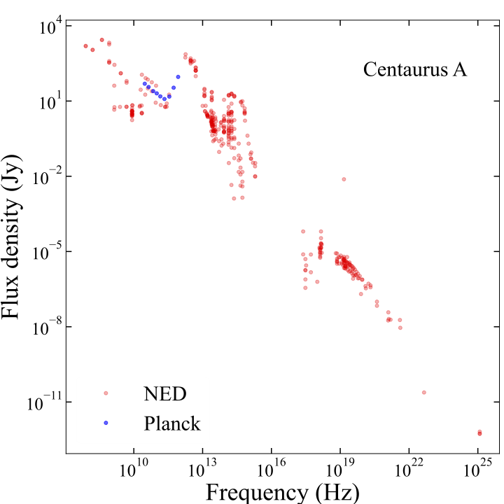
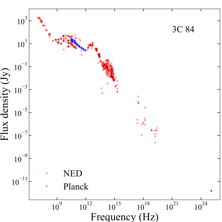
Figure 15: Spectral energy distribution (SED) for a few sources: red points are photometry from NED and the blue points are our Planck observations. The Planck data for Cen A add some new spectral coverage and help to define the rise of the dust component.

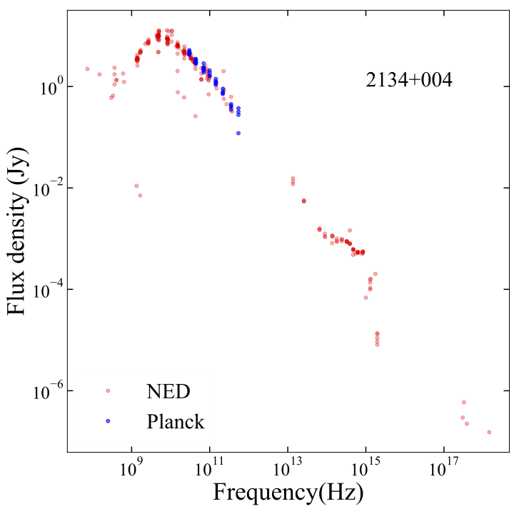
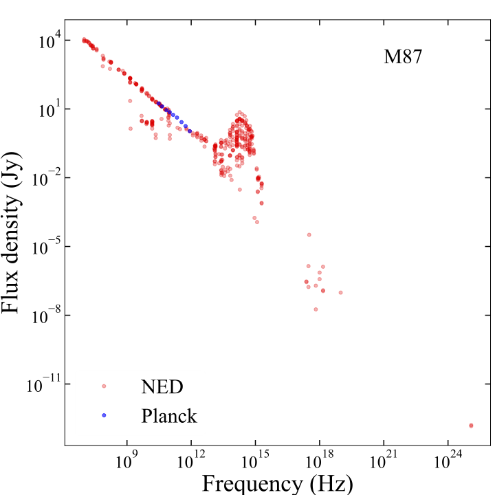
Figure 16: Spectral energy distribution (SED) for a few sources: red points are photometry from NED and the blue points are our Planck observations. The Planck observations of 2134+004 and M87 show good agreement with previous measurements.

6 Summary

In this paper we have introduced the new Planck Catalog of Polarized and Variable Compact Sources, PCCS-PV, comprising 153 sources, the majority of which are extragalactic, measured in both total power and polarization by Planck, with frequency coverage from 30 to 353 GHz, and time-scales ranging from days to years. We classify 135 of the 153 sources as beamed, extragalactic radio sources (blazars), four as well-studied radio galaxies such as 3C 84 and M87, and 14 as Galactic or Magellanic Cloud sources, including H ii regions, planetary nebulae, etc. To allow an assessment of variability of polarized sources, the catalog was generated using an advanced extraction method, tod2flux, applied directly to the multifrequency Planck time-ordered data, rather than the mission sky maps. We used the calibrated timelines from the Planck NPIPE data release, PR4, as input to our processing.

To check our measurements and to illustrate possible uses of our catalog, we have compared the Planck polarization data of selected objects with published data from other astronomical instruments. Our preliminary findings show that for the selected sources OJ 287 and 3C 454.3, the flux densities at 30 and 44 GHz agree with the Metsähovi 37 GHz values at nearby epochs, while there is general correspondence between the Planck and IRAM polarization. This general agreement confirms our measurements. Furthermore we have found that the Planck polarization of OJ 287 is similar to that of the core, supporting the conclusion of Sasada et al. (2018) that the optical polarization is related to that of the core at some epochs and the knot at others. From joint analysis of our data and optical R-band data, we have shown a strong frequency dependency of the degree of polarization and EVPA of 3C 454.3, with the EVPA at the highest Planck frequencies becoming similar to the optical EVPA during the early stages of a major outburst. This has led us to conclude that the optical flare during the first Planck survey in late 2009 occurred within the same region as the 200 GHz flare, which is distinct from the regions that dominate the emission at lower frequencies.

We have also presented Planck data along with observations compiled in NED for five non-blazar extragalactic sources to demonstrate Planck’s contribution to the overall SED of the sources. Planck observations of M87 and the quasar 2134+004 are in good agreement with the observations in NED, confirming the flux density calibration of the Planck data. For the remaining three sources, Centaurus A, 3C 84, and Pictor A, the Planck data help to fill in missing spectral coverage. In particular, in Centaurus A, the Planck data help to define the rise as the infrared dust component starts to dominate the spectrum.

These preliminary results illustrate the usefulness of our Planck catalog, PCCS-PV, for application with follow-up studies. Furthermore, our versatile ToD-based flux-fitting software, tod2flux, is applicable to other experimental data sets.

PCCS-PV will be available at the ESA Planck Legacy Archive. and at the NASA/IPAC Infrared Science Archive., while the flux-fitting algorithm, tod2flux, is released as open source software.

Software used in this work

Astropy (Astropy Collaboration et al., 2013, 2018), HEALPix (Górski et al., 2005), Matplotlib (Hunter, 2007; Caswell et al., 2021), Numpy (Harris et al., 2020), TOAST, and Scipy (Virtanen et al., 2020).

Appendix A Sample catalog file

We show an example of a catalog file in Table 3. This one is for PCCS2 143 G009.33$-$19.61, better known as QSO B1921$-$293. These results combine two adjacent frequency bands to boost the signal-to-noise ratio of each entry.

Table 3: Sample catalog file extract.

# Target = PCCS2 143 G009.33-19.61 a.k.a. QSO B1921-293 -- BL Lac - type object
# band(s)     , freq [GHz],      start,       stop, I flux [mJy], I error [mJy], Q flux [mJy], Q error [mJy], U flux [mJy], U error [mJy],    Pol.Frac,    PF low lim,  PF high lim, Pol.Ang [deg],   PA low lim,   PA high lim
       30+44,       32.182, 2009-09-29, 2009-10-06,      16000.0,          69.8,        -33.5,          94.8,       -136.1,          99.6,       0.0066,       0.0000,       0.0197,       -51.907,   -146.663,     42.720
       44+70,       58.818, 2009-10-04, 2009-10-05,      13443.3,         110.7,         51.9,         142.7,       -332.0,         175.5,       0.0225,       0.0009,       0.0485,       -40.555,    -70.395,     -0.150
      70+100,       96.610, 2009-10-03, 2009-10-04,      11271.7,          49.7,       -229.0,          74.7,         69.0,          73.1,       0.0202,       0.0086,       0.0339,        81.613,     63.813,     99.570
     100+143,      131.311, 2009-09-30, 2009-10-01,       9582.8,          27.0,       -117.7,          52.0,         83.7,          49.3,       0.0141,       0.0048,       0.0253,        72.301,     50.353,     92.881
     143+217,      167.344, 2009-10-02, 2009-10-03,       8157.3,          25.4,         55.0,          54.6,         60.4,          55.0,       0.0074,       0.0000,       0.0220,        23.858,    -84.555,    132.337
     217+353,      246.339, 2009-10-02, 2009-10-02,       6152.8,          39.5,         75.5,          69.5,       -102.6,          85.6,       0.0165,       0.0000,       0.0443,       -26.813,   -122.771,     69.173
     353+545,      430.560, 2009-10-01, 2009-10-02,       4169.6,          66.2,        315.2,         196.0,       -278.2,         182.7,       0.0907,       0.0102,       0.1924,       -20.717,    -53.489,      8.537
     545+857,      700.023, 2009-10-02, 2009-10-02,       2887.4,          70.8,          0.0,           0.0,          0.0,           0.0,       0.0000,       0.0000,       0.0000,         0.000,      0.000,      0.000
       30+44,       32.196, 2010-04-03, 2010-04-10,      15476.6,          68.4,       -539.3,          97.6,       -695.0,          95.4,       0.0565,       0.0448,       0.0686,       -63.906,    -69.335,    -58.331
       44+70,       57.373, 2010-04-04, 2010-04-05,      13108.5,         116.8,       -522.7,         153.6,       -745.5,         187.5,       0.0685,       0.0423,       0.0965,       -62.518,    -72.334,    -53.659
      70+100,       97.784, 2010-04-05, 2010-04-06,      10769.2,          46.0,       -488.5,          66.3,       -645.7,          71.4,       0.0749,       0.0634,       0.0872,       -63.553,    -68.112,    -59.239
     100+143,      129.550, 2010-04-08, 2010-04-09,       9214.9,          26.0,       -398.7,          45.5,       -507.1,          46.6,       0.0698,       0.0613,       0.0791,       -64.088,    -67.866,    -60.300
     143+217,      170.622, 2010-04-06, 2010-04-07,       7651.2,          24.1,       -301.8,          50.8,       -421.1,          49.5,       0.0674,       0.0560,       0.0794,       -62.816,    -68.104,    -57.499
     217+353,      244.762, 2010-04-07, 2010-04-07,       5886.6,          35.4,       -255.1,          76.6,       -396.1,          79.8,       0.0789,       0.0554,       0.1047,       -61.390,    -70.330,    -52.671
     353+545,      424.983, 2010-04-08, 2010-04-08,       4079.1,          63.5,        -94.1,         190.9,       -592.2,         197.1,       0.1393,       0.0560,       0.2371,       -49.517,    -68.426,    -31.301
     545+857,      719.622, 2010-04-08, 2010-04-08,       2799.4,          65.7,          0.0,           0.0,          0.0,           0.0,       0.0000,       0.0000,       0.0000,         0.000,      0.000,      0.000
       30+44,       32.800, 2010-09-29, 2010-10-06,      13487.8,          74.0,       -808.2,         100.7,       -908.7,         107.2,       0.0898,       0.0758,       0.1045,       -65.825,    -70.246,    -61.398
       44+70,       56.334, 2010-10-04, 2010-10-05,      10946.6,         117.3,       -550.9,         147.2,       -754.9,         192.6,       0.0839,       0.0569,       0.1142,       -63.060,    -73.898,    -54.073
      70+100,       97.415, 2010-10-03, 2010-10-04,       8374.8,          50.4,       -403.7,          76.9,       -470.8,          76.1,       0.0734,       0.0584,       0.0898,       -65.307,    -72.235,    -58.341
     100+143,      131.224, 2010-09-30, 2010-10-01,       6723.2,          27.1,       -375.2,          48.9,       -375.2,          47.2,       0.0786,       0.0663,       0.0917,       -67.499,    -72.366,    -62.452
     143+217,      171.378, 2010-10-02, 2010-10-03,       5538.4,          24.7,       -285.7,          50.1,       -328.1,          49.9,       0.0780,       0.0620,       0.0951,       -65.524,    -71.573,    -59.446
     217+353,      247.381, 2010-10-02, 2010-10-02,       4225.1,          35.2,       -145.5,          70.3,       -266.3,          79.1,       0.0697,       0.0381,       0.1058,       -59.323,    -73.573,    -46.672
     353+545,      434.882, 2010-10-01, 2010-10-02,       2879.9,          58.0,       -216.3,         209.6,         -7.7,         186.9,       0.0376,       0.0000,       0.1939,       -88.981,   -191.752,     13.857
     545+857,      676.404, 2010-10-01, 2010-10-02,       2002.6,          62.2,          0.0,           0.0,          0.0,           0.0,       0.0000,       0.0000,       0.0000,         0.000,      0.000,      0.000
       30+44,       32.419, 2011-04-03, 2011-04-10,      14244.5,          69.4,        326.6,          97.0,       -838.6,          97.8,       0.0628,       0.0510,       0.0755,       -34.361,    -40.128,    -28.505
       44+70,       58.093, 2011-04-04, 2011-04-05,      11569.0,         111.9,        200.3,         148.0,       -538.9,         170.4,       0.0478,       0.0235,       0.0766,       -34.807,    -48.958,    -17.658
      70+100,       97.611, 2011-04-05, 2011-04-06,       9406.2,          42.7,         66.5,          60.5,       -343.7,          69.8,       0.0367,       0.0231,       0.0512,       -39.524,    -49.208,    -30.093
     100+143,      128.005, 2011-04-08, 2011-04-09,       7908.3,          25.8,        106.8,          41.4,       -314.2,          46.4,       0.0416,       0.0310,       0.0530,       -35.615,    -42.292,    -28.686
     143+217,      174.305, 2011-04-06, 2011-04-07,       6387.1,          24.0,         67.5,          45.6,       -311.5,          48.3,       0.0494,       0.0362,       0.0638,       -38.890,    -46.535,    -30.882
     217+353,      242.701, 2011-04-07, 2011-04-07,       5053.1,          33.7,          8.8,          70.0,       -235.7,          71.2,       0.0446,       0.0199,       0.0732,       -43.936,    -61.493,    -27.401
     353+545,      425.582, 2011-04-08, 2011-04-08,       3366.3,          60.2,        170.5,         192.9,         60.8,         166.7,       0.0000,       0.0000,       0.1976,         9.819,   -130.564,    150.214
     545+857,      731.062, 2011-04-08, 2011-04-08,       2210.1,          60.8,          0.0,           0.0,          0.0,           0.0,       0.0000,       0.0000,       0.0000,         0.000,      0.000,      0.000
       30+44,       32.976, 2011-09-26, 2011-10-05,      14861.0,          61.4,        221.1,          77.2,      -1337.1,         101.0,       0.0911,       0.0786,       0.1037,       -40.305,    -43.258,    -37.292
       44+70,       55.448, 2011-10-02, 2011-10-04,      12614.1,          98.2,         -3.7,         128.8,       -966.9,         170.6,       0.0760,       0.0516,       0.1024,       -45.108,    -51.725,    -36.989
      70+100,       98.052, 2011-10-01, 2011-10-02,      10435.2,          39.5,       -165.8,          56.8,       -690.4,          61.8,       0.0678,       0.0572,       0.0790,       -51.753,    -55.985,    -47.497
     100+143,      131.682, 2011-09-27, 2011-09-28,       8835.1,          20.1,       -105.1,          36.7,       -588.2,          39.6,       0.0675,       0.0594,       0.0759,       -50.066,    -53.355,    -46.822
     143+217,      167.716, 2011-09-30, 2011-10-01,       7504.9,          18.6,        -88.0,          40.5,       -457.2,          43.0,       0.0618,       0.0515,       0.0728,       -50.446,    -54.913,    -45.827
     217+353,      240.365, 2011-09-29, 2011-09-30,       5802.6,          29.6,       -121.8,          61.4,       -253.7,          68.7,       0.0474,       0.0258,       0.0714,       -57.825,    -70.148,    -45.794
     353+545,      424.828, 2011-09-29, 2011-09-29,       4059.3,          57.1,       -166.5,         160.6,        -46.2,         174.9,       0.0027,       0.0000,       0.1124,       -82.245,   -222.468,     57.955
     545+857,      726.542, 2011-09-29, 2011-09-29,       2705.3,          57.7,          0.0,           0.0,          0.0,           0.0,       0.0000,       0.0000,       0.0000,         0.000,      0.000,      0.000
       30+44,       31.721, 2012-04-05, 2012-04-15,      12390.7,          51.6,        394.2,          71.0,      -1167.3,          73.3,       0.0993,       0.0888,       0.1100,       -35.671,    -38.737,    -32.585
       44+70,       58.491, 2012-04-06, 2012-04-08,       9759.9,          96.0,         31.9,         120.7,       -726.8,         155.4,       0.0735,       0.0452,       0.1037,       -43.743,    -53.242,    -34.629
       30+44,       30.997, 2012-10-03, 2012-10-05,      12778.7,          66.2,        909.7,          84.5,       -899.2,         104.7,       0.0998,       0.0861,       0.1143,       -22.335,    -26.058,    -18.493
       44+70,       63.664, 2012-10-01, 2012-10-03,       9027.2,         119.1,        732.3,         162.2,       -319.6,         195.3,       0.0855,       0.0587,       0.1182,       -11.788,    -25.542,      1.262
       30+44,       33.001, 2013-04-05, 2013-04-16,       7308.8,          57.0,          0.3,          78.1,       -305.9,          83.8,       0.0405,       0.0204,       0.0633,       -44.971,    -60.112,    -31.039
       44+70,       56.412, 2013-04-07, 2013-04-09,       5726.6,          88.7,       -104.8,         112.4,        152.7,         142.4,       0.0241,       0.0000,       0.0741,        62.229,    -44.755,    168.972

References

- Agudo et al. (2018) Agudo, I., Thum, C., Ramakrishnan, V., et al. 2018, MNRAS, 473, 1850
- Astropy Collaboration et al. (2018) Astropy Collaboration, Price-Whelan, A. M., Sipőcz, B. M., et al. 2018, AJ, 156, 123
- Astropy Collaboration et al. (2013) Astropy Collaboration, Robitaille, T. P., Tollerud, E. J., et al. 2013, A&A, 558, A33
- Begelman et al. (1984) Begelman, M. C., Blandford, R. D., & Rees, M. J. 1984, Reviews of Modern Physics, 56, 255
- Blandford et al. (2019) Blandford, R., Meier, D., & Readhead, A. 2019, ARA&A, 57, 467
- Caswell et al. (2021) Caswell, T. A., Droettboom, M., Lee, A., et al. 2021, matplotlib/matplotlib: REL: v3.4.2
- Chen et al. (2013) Chen, X., Rachen, J. P., López-Caniego, M., et al. 2013, A&A, 553, A107
- Croton et al. (2006) Croton, D. J., Springel, V., White, S. D. M., et al. 2006, MNRAS, 365, 11
- Datta et al. (2019) Datta, R., Aiola, S., Choi, S. K., et al. 2019, MNRAS, 486, 5239
- Fabian (2012) Fabian, A. C. 2012, ARA&A, 50, 455
- Giovannini et al. (2018) Giovannini, G., Savolainen, T., Orienti, M., et al. 2018, Nature Astronomy, 2, 472
- Górski et al. (2005) Górski, K. M., Hivon, E., Banday, A. J., et al. 2005, ApJ, 622, 759
- Hada et al. (2011) Hada, K., Doi, A., Kino, M., et al. 2011, Nature, 477, 185
- Harris et al. (2020) Harris, C. R., Millman, K. J., van der Walt, S. J., et al. 2020, Nature, 585, 357
- Helou et al. (1995) Helou, G., Madore, B. F., Schmitz, M., et al. 1995, The NASA/IPAC Extragalactic Database, ed. D. Egret & M. A. Albrecht, Vol. 203, 95
- Hunter (2007) Hunter, J. D. 2007, Computing in Science & Engineering, 9, 90
- Jorstad et al. (2017) Jorstad, S. G., Marscher, A. P., Morozova, D. A., et al. 2017, ApJ, 846, 98
- Jorstad et al. (2013) Jorstad, S. G., Marscher, A. P., Smith, P. S., et al. 2013, ApJ, 773, 147
- Junor et al. (1999) Junor, W., Biretta, J. A., & Livio, M. 1999, Nature, 401, 891
- King & Pounds (2015) King, A. & Pounds, K. 2015, ARA&A, 53, 115
- Magorrian et al. (1998) Magorrian, J., Tremaine, S., Richstone, D., et al. 1998, AJ, 115, 2285
- Montier et al. (2015) Montier, L., Plaszczynski, S., Levrier, F., et al. 2015, A&A, 574, A136
- Partridge et al. (2017) Partridge, B., Bonavera, L., López-Caniego, M., et al. 2017, Galaxies, 5, 47
- Planck Collaboration XIII (2011) Planck Collaboration XIII. 2011, A&A, 536, A13
- Planck Collaboration XIV (2011) Planck Collaboration XIV. 2011, A&A, 536, A14
- Planck Collaboration I (2014) Planck Collaboration I. 2014, A&A, 571, A1
- Planck Collaboration IX (2014) Planck Collaboration IX. 2014, A&A, 571, A9
- Planck Collaboration XXVI (2016) Planck Collaboration XXVI. 2016, A&A, 594, A26
- Planck Collaboration I (2020) Planck Collaboration I. 2020, A&A, 641, A1
- Planck Collaboration II (2020) Planck Collaboration II. 2020, A&A, 641, A2
- Planck Collaboration III (2020) Planck Collaboration III. 2020, A&A, 641, A3
- Planck Collaboration Int. XLV (2016) Planck Collaboration Int. XLV. 2016, A&A, 596, A106
- Planck Collaboration Int. LIV (2018) Planck Collaboration Int. LIV. 2018, A&A, 619, A94
- Planck Collaboration Int. LVII (2020) Planck Collaboration Int. LVII. 2020, A&A, 643, 42
- Sasada et al. (2018) Sasada, M., Jorstad, S., Marscher, A. P., et al. 2018, ApJ, 864, 67
- Virtanen et al. (2020) Virtanen, P., Gommers, R., Oliphant, T. E., et al. 2020, Nature Methods, 17, 261
- Wenger et al. (2000) Wenger, M., Ochsenbein, F., Egret, D., et al. 2000, A&AS, 143, 9