Modifying the Asynchronous Jacobi Method for Data Corruption Resilience.

Abstract

Moving scientific computation from high-performance computing (HPC) and cloud computing (CC) environments to devices on the edge, where data can be collected by streamlined computing devices that are physically located near instruments of interest, has received tremendous interest in recent years. Such edge computing environments can operate on data in-situ instead of requiring the collection of data in HPC and/or CC facilities, offering enticing benefits that include avoiding costs of transmission over potentially unreliable or slow networks, increased data privacy, and real-time data analysis. Before such benefits can be realized at scale, new fault tolerant approaches must be developed to address the inherent unreliability of edge computing environments, because the traditional resilience approaches used by HPC and CC are not generally applicable to edge computing. Those traditional approaches commonly utilize checkpoint-and-restart and/or redundant-computation strategies that are not feasible for edge computing environments where data storage is limited and synchronization is expensive. Motivated by prior algorithm-based fault tolerance approaches, a variant of the asynchronous Jacobi (ASJ) method is developed herein with resilience to data corruption achieved by leveraging existing convergence theory. The proposed ASJ variant rejects solution approximations from neighbor devices if the distance between two successive approximations violates an analytic bound. Numerical results show the ASJ variant restores convergence in the presence of certain types of natural and malicious data corruption.

1 Introduction

Recent years have seen a proliferation of edge devices, i.e., streamlined computing devices that provide an entry point to the individual instruments in their vicinity. Modern infrastructure includes a wide range of such devices, from smart residential thermostats to industrial smart grid meters. These devices, along with wearable healthcare devices and content delivery systems, are motivating a push of computation beyond the walls of high-performance (HPC) and cloud computing (CC) facilities onto the edge devices themselves. Consider, as an example, the benefits of enabling smart power grid devices to operate autonomously when the central operator is disabled due to a natural disaster or cyber-physical attack. The capability provided by edge computing environments to operate without a single point of failure or on data in-situ is appealing to real-time system operators. Unfortunately, the benefits of edge computing cannot be realized before the inherent unreliability of edge devices is addressed. Modern scientific computing algorithms typically assume that data will not be corrupted as the algorithm is executed. HPC and CC platforms provide such data integrity by utilizing fault management techniques. Checkpointing and redundant computation are cornerstones of fault management techniques in HPC and CC, and are an integral part of n-modular redundancy [5], n-version programming [12], majority voting [5], and redundant cloud servers [12] techniques. The frequency of checkpointing is typically chosen to avoid restarting from a checkpoint created long before the fault occurs while keeping the cost of synchronization and storage reasonable. Similarly, the amount of redundancy is typically chosen to avoid having all redundant entities experience a fault at the same time while keeping the cost of storage and flops reasonable. Thus, flop and storage limitations, along with heterogeneity of devices, can make checkpointing and redundancy too expensive for practical use in edge computing environments.

One promising alternative fault management strategy is the class of algorithm based fault tolerant (ABFT) methods. The general idea is to leverage the structure or expected behavior of the algorithm to detect, mitigate, and/or recover from faults such as data corruption. Examples of ABFT schemes include methods for the fast Fourier transform [11], matrix multiplication [16], Krylov-based iterative methods [7], and the synchronous Jacobi method [2]. Focusing on the iterative methods, the work presented in [7] uses the orthogonality of projections onto Krylov spaces for detection of faults, while [2] utilizes the contraction mapping property of stationary iterative methods. Unfortunately, those ABFT approaches are for iterative methods that require frequent synchronizations, making them impractical for edge computing environments due to network latency, heterogeneous nodes, and nonpersistent nodes/links. Alternatively, ABFT approaches for asynchronous methods, such as linear systems solvers and optimization algorithms, remove the need for global synchronization after each iteration. The authors are aware of only two existing asynchronous methods with ABFT strategies: the robust alternating direction method of multipliers (ADMM) [10] and the robust push-sum algorithm [13].

To address the need for ABFT iterative methods for solving linear systems, we modify the asynchronous Jacobi iteration [8, 9, 15, 2, 6] with a resilience modification technique that has been employed in [10], where ADMM convergence theory is used to reject corrupted data from neighboring nodes. Here, the theoretical analysis for the asynchronous Jacobi method in [9] is used to establish a rejection criterion based on the difference between successive data obtained from neighboring nodes. Although the Jacobi method is known to scale poorly to large and ill-conditioned systems, which are limitations inherited by the asynchronous Jacobi method, the method is often a core building block underlying more scalable solvers and is, in fact, often sufficient for many small problems that appear in edge environments. For these reasons, it is a logical first step in developing asynchronous ABFT methods for solving linear systems.

This paper is organized as follows. Section 2 formulates the problem, introduces the notation and important definitions, and discusses the nature of data corruption to be investigated. Section 3 proposes our resilience enabling technique. Section 4 presents numerical results verifying the implementation of the method and demonstrating the effectiveness of the proposed rejection technique in the presence of various forms of data corruption. Section 5 summarizes the outcomes of the paper and discusses ongoing work.

2 Problem Statement

Solutions of linear systems are ubiquitous in modern scientific computing algorithms, defining search directions in both iterative and nonlinear solvers. Thus, consider solving the linear system

(1) $$A\mathbf{x}=\mathbf{b},$$

for $\mathbf{x}\in\mathbb{R}^{m}$, where $A\in\mathbb{R}^{m\times m}$ and $\mathbf{b}\in\mathbb{R}^{m}$. The asynchronous Jacobi method is an iterative solver for (1) in that successive approximations to the solution $\mathbf{x}$ are formed across $N$ computational nodes. Denote by $\mathbf{x}_{i}\in\mathbb{R}^{m_{i}}$, $m_{i}\leq m$, the partition of $\mathbf{x}$ that node $i$ is approximating. Let $I\in\mathbb{R}^{m\times m}$ and $D\in\mathbb{R}^{m\times m}$ be the identity matrix and the diagonal matrix containing the diagonal elements of $A$, respectively. The update equation that defines the successive approximations computed by node $i$, denoted $\mathbf{x}_{i}^{0}$, $\mathbf{x}_{i}^{1}$, etc., can now be expressed as

(2) $$\mathbf{x}_{i}^{\kappa}=\sum_{j=1}^{N}M_{ij}\mathbf{x}_{j}^{\psi(i,j,\kappa)}+\mathbf{c}_{i},\quad\kappa=1,2,\ldots$$

where $M_{ij}\in\mathbb{R}^{m_{i}\times m_{j}}$ is the $(i,j)$-th block of the Jacobi iteration matrix $M:=I-D^{-1}A$, $\mathbf{c}_{i}\in\mathbb{R}^{m_{i}}$ is the $i$-th block of $\mathbf{c}:=D^{-1}\mathbf{b}$, and $\psi(i,j,\kappa)=\lambda$ if node $i$ uses node $j$’s $\lambda$-th approximation in the computation of its $\kappa$-th approximation. The general form of (2) defines a class of chaotic or asynchronous iterative methods, first introduced by Chazan and Miranker [6], that generalize classic relaxation methods to allow each compute node to perform a new iteration immediately after the previous iteration has completed. Chazan and Miranker provide the sufficient condition to guarantee convergence of any relaxation scheme of the form (2): that the spectral radius of the absolute value of the global iteration matrix, $M$, is bounded below one, i.e., $\rho(|M|)<1$, where $|M|$ is defined by taking the absolute value of each element in the matrix. However, the authors in [6] assume that the values of $\mathbf{x}_{j}^{\psi(i,j,\kappa)}$ sent by node $j$ are the same as those received by node $i$. Such assumption can become invalid in emerging computing environments that do not provide the guarantees of current high performance computing systems. Thus, the goal of this work is to modify (2) to ensure, or at least encourage, convergence even if data corruption results in either (i) the values of $\mathbf{x}_{j}^{\psi(i,j,\kappa)}$ received by node $i$ being different than those sent by node $j$ or (ii) the values of $\mathbf{x}_{j}^{\kappa}$ stored on node $j$ being altered. As a convenience to the reader, Table 1 summarizes the notation used herein, as well as the location where the notation is first mentioned.

Table 1: Notation Table

Symbol Description Location $N$ number of computational nodes Section 2 $A$ square system matrix with real components, $\mathbb{R}^{m\times m}$ Section 2 $D$ diagonal matrix whose elements are the diagonal entries of $A$, $\mathbb{R}^{m\times m}$ Section 2 $M$ Jacobi iteration matrix $D^{-1}A$, $\mathbb{R}^{m\times m}$ Section 2 $M_{i,j}$ $(i,j)$-th block of $M$, $\mathbb{R}^{m_{i}\times m_{j}}$ Section 2 i,j,k blocks/elements Section 2 $\lambda,\kappa$ iteration number Section 2 $\mathbf{x}$ , $\mathbf{b}$ vectors of real components $\mathbb{R}^{m}$ Section 2 $\mathbf{x}_{i}$ vector containing the $i$-th block of elements of vector $\mathbf{x}$ (assume that the $i$-th node is in charge of the $i$-th block of $\mathbf{x}$) Section 2 $\mathbf{x}_{i,k}$ the $k$-th element of the vector $\mathbf{x}_{i}$ containing the $i$-th block of elements of vector $\mathbf{x}$ Section 2 $\mathbf{x}_{i}^{\kappa}$ the $\kappa$-th iteration of the $i$-th block of elements of vector $\mathbf{x}$ Section 2 $p$ the probability of a bit flip in a communicated element Section 2.1 $\omega_{f}$, $\omega_{r}$ the time to failure and recovery time Section 2.2 $\delta$ an offset that is sampled from a Gaussian distribution with a positive mean Section 2.2 $\nu_{i}(t)$ the iteration index on node $i$ such that $\mathbf{x}_{i}^{\nu_{i}(t)}$ is the most recent approximation of $\mathbf{x}_{i}$ at time $t$ Section 3 $\widetilde{\mathbf{x}}(t)$ global approximate solution at time $t$ such that $\mathbf{\widetilde{x}}_{i}(t)=\mathbf{x}_{i}^{\nu_{i}(t)}$, $i=1,\ldots,N$ Section 3 $\mathbf{x}^{*}$ global exact solution to $A\mathbf{x}=\mathbf{b}$ Section 3 $\mathbf{e}(t)$ global error at time $t$ such that $\mathbf{e}_{i}(t)=\widetilde{\mathbf{x}}_{i}(t)-\mathbf{x}_{i}^{*}$ Section 3 $\Omega(t):=\Omega(\psi,M,t)$ error operator st $\mathbf{e}(t)=\Omega(t)\mathbf{e}(0)$ Section 3 $\mathcal{G}(\mathcal{V},\mathcal{E})$ directed acyclic graph with nodes $\mathcal{V}$ and edges $\mathcal{E}$ Section 3 $s(t)$, $l(t)$ shortest and longest paths in $\mathcal{G}$, respectively Section 3 $\psi_{ij}(\kappa):=\psi(i,j,\kappa)$ index of the update from node $j$ which node $i$ uses to compute its $\kappa$-th update Section 3 $\zeta_{ij}(t)$ $\arg\max_{\kappa}{\psi_{ij}(\kappa)<\psi_{ij}(\nu_{i}(t))}$ Section 3 $\tau_{ij}[\kappa]$ time at which the solution approximation existed on node $j$ that will later be used to form $\mathbf{x}_{i}^{\kappa}$ Section 3 $\sigma_{min}(A),\sigma_{max}(A)$ smallest and largest singular value of $A$ Section 3 $\tilde{s}_{i}(t)$ approximate shortest path Section 3 $d\mathbf{x}_{i}^{\nu_{i}(t)}:=\mathbf{x}_{i}^{\nu_{i}(t)}-\mathbf{x}_{i}^{\nu_{i}(t)-1}$ difference between two successive updates from the $i$-th block of elements Section 3 $\epsilon$ a user defined tolerance for the stopping criteria Section 3 $\kappa(A)$ condition number of matrix $A$ Section 3

2.1 Natural Data Corruption

The first data corruption model is motivated by bit flips occurring in network hardware memory that alter data as it is in transit. This natural data corruption is modeled as a random process where each component of transmitted data is affected by a bit flip with a fixed probability $p\in(0,1)$. The bit flips themselves are performed either on ieee 754 double precision (64 bit) floating point [1] or on 32 bit signed integer numbers. The affected bit index is sampled from various uniform integer distributions, then the bit flip is performed directly. In extremely rare cases, this method of performing bit flips on double precision numbers can result in the special floating point values NaN or inf. It is worth noting that this data corruption approach mirrors the model of Anzt et al. [2]. Anzt et al. introduce a fixed number of bit flips per iteration to the entries of the iteration matrix $M$ during the matrix-vector product in each iteration, which may corrupt up to $1\%$ of updates to the elements of the solution vector. Instead, we choose to corrupt the elements of the transmitted solution vector directly at a fixed probability $p\in(0,1)$, i.e., corruption is applied with probability $p$ to each transmitted data element.

2.2 Malevolent Data Corruption

The second data corruption model is motivated by intentional corruption caused by a malicious actor who has gained intermittent access to a device to manipulate the result of a calculation. This malevolent data corruption is modeled as a periodic process where each agent is considered to be in either a “normal” or a “degraded” state. When in a “normal” state, the new approximate solution is unaltered. After $\omega_{f}$ seconds have passed, the agent is compromised and enters a “degraded” state. While in the “degraded” state, the impacted data on an agent is corrupted by adding an offset to all solution elements. Note that such non-transient corruption, i.e., overwriting of the local solution data, presents a more challenging recovery scenario than transient corruption. This offset is sampled from a Gaussian distribution with a positive mean $\delta$ and a standard deviation of $0.5\delta$. The repeated application of these offsets will gradually increase the magnitude of the corrupted elements of the solution vector, absent any mitigation strategy. We choose the standard deviation $0.5\delta$ to ensure that $95\%$ of the sampled offsets will be greater than zero regardless of the choice of $\delta$. After $\omega_{r}$ seconds have passed, the agent is secured and returns to a “normal” state.

3 Modification Formulation

To improve data corruption resilience in the asynchronous Jacobi method (2), we take the approach of inspecting incoming data before it is used to form the next approximation $\mathbf{x}_{i}^{\kappa}$ in (2). If the data is identified as corrupted, it is rejected by being excluded from contributing to the next solution approximation. We will use the convergence theory established by Hook and Dingle [9] to derive our rejection criterion. The authors in [9] derive an error bound using metrics of the evolution of the solution approximations computed by each node and the communication pattern between nodes. They accomplish this task by casting the algorithm evolution as a directed acyclic graph, whose vertices are the solution approximations computed by each node and edges indicate when a solution approximation is used to compute a latter solution approximation. Using a similar notation, we will summarize the components used to form the rejection criterion below.

Define $\nu_{i}(t)$ so that $\mathbf{x}_{i}^{\nu_{i}(t)}$ is the solution approximation on node $i$ at time $t$. A global solution approximation at time $t$, denoted by $\mathbf{\widetilde{x}}(t)$, is defined block-wise as $\mathbf{\widetilde{x}}_{i}(t)=\mathbf{x}_{i}^{\nu_{i}(t)}$, $i=1,\ldots,N$. With $\mathbf{x}^{*}$ being the exact solution of (1), the global error at time $t$ is defined as $\mathbf{e}(t)=\mathbf{\widetilde{x}}(t)-\mathbf{x}^{*}$. Denote the error operator $\Omega(\psi,M,t)$ such that $\mathbf{e}(t)=\Omega(\psi,M,t)\mathbf{e}(0)$. The properties of $\Omega(\psi,M,t)$, denoted herein as $\Omega(t)$, are presented in [9] using a directed acyclic graph $\mathcal{G}(\mathcal{V},\mathcal{E})$ with graph nodes $\mathcal{V}$ and edges $\mathcal{E}$. This is not the graph of computational node-to-node connections but is instead a directed acyclic graph representation of the evolution of the collective computation: each solution approximation at each computational node (i.e., each $\mathbf{x}_{j}^{\kappa}$) is an element of $\mathcal{V}$, and there is an edge in $\mathcal{E}$ from $\mathbf{x}_{j}^{\lambda}$ to $\mathbf{x}_{i}^{\kappa}$ iff $\psi(i,j,\kappa)=\lambda$. Figure 1 represents a simple example of a potential directed acyclic graph for the algorithm evolution between two nodes. The initial states of processors are denoted by $\mathbf{x}_{1}^{0}$ and $\mathbf{x}_{2}^{0}$, respectively. The initial solution approximation for node 2, $\mathbf{x}_{2}^{0}$, is received by node 1 and used to compute the next solution approximation for node 1, $\mathbf{x}_{1}^{1}$:

$$\mathbf{x}_{1}^{1}=M_{11}\mathbf{x}_{1}^{0}+M_{12}\mathbf{x}_{2}^{0}.$$

Node 2, on the other hand, uses $\mathbf{x}_{1}^{1}$ instead of $\mathbf{x}_{1}^{0}$ to compute the next approximation

$${\bm{x}}_{2}^{1}=M_{22}{\bm{x}}_{2}^{0}+M_{12}{\bm{x}}_{1}^{1},$$

as depicted in Figure 1. Hook and Dingle [9, Theorem 1] prove that the error operator $\Omega(\psi,M,t)$ is a sum over all the paths within $\mathcal{G}(\mathcal{V},\mathcal{E})$ of the corresponding iteration matrix blocks. For example, the error operator at time $t_{1}$ in Figure 1 is

$$\Omega(\psi,M,t_{1})=\begin{bmatrix}M_{11}M_{11}M_{11}+M_{12}M_{21}M_{11}&M_{12}M_{22}+M_{11}M_{12}\\ M_{22}M_{21}M_{11}+M_{21}M_{11}&M_{22}M_{22}+M_{21}M_{12}+M_{22}M_{21}M_{12}\end{bmatrix}.$$

The authors further show that the convergence rate is bounded by the slowest propagation of information, defined as the shortest path in $\mathcal{G}(\mathcal{V},\mathcal{E})$ from an initial solution approximation to a current approximation, leading to the error bound that forms the basis of our rejection criteria.

Figure 1: Directed acyclic graph $\mathcal{G}(\mathcal{V},\mathcal{E})$ illustrating an example two-node evolution of the solution approximations $\mathbf{x}_{1}^{\nu_{1}(t)}$ and $\mathbf{x}_{2}^{\nu_{2}(t)}$.

Given a non-negative iteration matrix $M$, i.e., all elements of $M$ are non-negative, Hook and Dingle [9, Theorem 3] show that $\Omega(t)$ is bounded as follows

(3) $$\|\Omega(t)\|_{2}\leq\left\|\sum_{k=s(t)}^{l(t)}M^{k}\right\|_{2},$$

where $s(t)$ and $l(t)$ are the lengths of the shortest and longest paths in $\mathcal{G}(\mathcal{V},\mathcal{E})$ at time $t$, respectively. The goal now is to use (3) to develop a criterion for whether computational node $i$ should accept or reject a new solution approximation $\mathbf{x}_{j}^{\psi(i,j,\nu_{i}(t))}$ obtained from node $j$. For notational brevity, we introduce $\psi_{ij}(\kappa):=\psi(i,j,\kappa)$.

To compare the new solution approximation $\mathbf{x}_{j}^{\psi_{ij}(\nu_{i}(t))}$ to the previous solution approximation received by computational node $i$ from computational node $j$, we define $\zeta_{ij}(t)$ to be the index of the solution approximation on node $i$ that was last directly influenced by a solution approximation from node $j$. In other words, we seek to denote the two most recent solution approximations received by node $i$ from node $j$ at time $t$ as $\mathbf{x}_{j}^{\psi_{ij}(\nu_{i}(t))}$ and $\mathbf{x}_{j}^{\psi_{ij}(\zeta_{ij}(t))}$, respectively. Formally, $\zeta_{ij}(t)=\arg\max_{\kappa}\{\psi_{ij}(\kappa)<\psi_{ij}(\nu_{i}(t))\}$. Now, a bound on $\|\mathbf{x}_{j}^{\psi_{ij}(\nu_{i}(t))}-\mathbf{x}_{j}^{\psi_{ij}(\zeta_{ij}(t))}\|_{2}$ can be derived using (3). Let $\tau_{ij}[\kappa]$ be the time at which the solution approximation existed on computational node $j$ that would later be used to form $\mathbf{x}_{i}^{\kappa}$, so that $\nu_{j}\big{(}\tau_{ij}[\zeta_{ij}(t)]\big{)}=\psi_{ij}(\zeta_{ij}(t))$ and $\nu_{j}\big{(}\tau_{ij}[\nu_{i}(t)]\big{)}=\psi_{ij}(\nu_{i}(t))$. Note that $\mathbf{x}_{j}^{\psi_{ij}(\nu_{i}(t))}$ can now be expressed as $\mathbf{x}_{j}^{\nu_{j}(\tau_{ij}[\nu_{i}(t)])}=\mathbf{\widetilde{x}}_{j}\big{(}\tau_{ij}[\nu_{i}(t)]\big{)}$ and $\mathbf{x}_{j}^{\psi_{ij}(\zeta_{ij}(t))}$ as $\mathbf{x}_{j}^{\nu_{j}(\tau_{ij}[\zeta_{ij}(t)])}=\mathbf{\widetilde{x}}_{j}\big{(}\tau_{ij}[\zeta_{ij}(t)]\big{)}$. Thus, the following bound holds

$$\mathbf{x}_{j}^{\psi_{ij}(\nu_{i}(t))}-\mathbf{x}_{j}^{\psi_{ij}(\zeta_{ij}(t))}=\underbrace{\mathbf{\widetilde{x}}_{j}\big{(}\tau_{ij}[\nu_{i}(t)]\big{)}-\mathbf{x}^{*}_{j}}_{\left[\Omega\big{(}\tau_{ij}[\nu_{i}(t)]\big{)}\mathbf{e}(0)\right]_{j}}+\underbrace{\mathbf{x}^{*}_{j}-\mathbf{\widetilde{x}}_{j}\big{(}\tau_{ij}[\zeta_{ij}(t)]\big{)}}_{\left[-\Omega\big{(}\tau_{ij}[\zeta_{ij}(t)]\big{)}\mathbf{e}(0)\right]_{j}}$$

$$\Rightarrow\|\mathbf{x}_{j}^{\psi_{ij}(\nu_{i}(t))}-\mathbf{x}_{j}^{\psi_{ij}(\zeta_{ij}(t))}\|_{2}\leq\bigg{[}\big{\|}\Omega\big{(}\tau_{ij}[\zeta_{ij}(t)]\big{)}\big{\|}_{2}+\big{\|}\Omega\big{(}\tau_{ij}[\nu_{i}(t)]\big{)}\big{\|}_{2}\bigg{]}\|\mathbf{e}(0)\|_{2}$$

Assuming the initial solution approximation is the zero vector, one has $\|\mathbf{e}(0)\|_{2}\leq\|A^{-1}\|_{2}\|\mathbf{b}\|_{2}$. Assuming also that the iteration matrix $M$ is non-negative, the Hook and Dingle bound (3) is now applied to obtain

(4) $$\|\mathbf{x}_{j}^{\psi_{ij}(\nu_{i}(t))}-\mathbf{x}_{j}^{\psi_{ij}(\zeta_{ij}(t))}\|_{2}\leq\bigg{[}\left\|\sum_{k=s(\tau_{ij}[\zeta_{ij}(t)])}^{l(\tau_{ij}[\zeta_{ij}(t)])}M^{k}\right\|_{2}+\left\|\sum_{k=s(\tau_{ij}[\nu_{i}(t)])}^{l(\tau_{ij}[\nu_{i}(t)])}M^{k}\right\|_{2}\bigg{]}\|A^{-1}\|_{2}\|\mathbf{b}\|_{2}.$$

Evaluating the bound (4) directly is very difficult in practice, primarily because none of $A^{-1}$, the $\tau_{ij}$ map, nor the $s(t)$ and $l(t)$ functions are known a priori. Thus, to obtain a practical version of (4), the two individual finite series are bounded by a single infinite series

$$\|\mathbf{x}_{j}^{\psi_{ij}(\nu_{i}(t))}-\mathbf{x}_{j}^{\psi_{ij}(\zeta_{ij}(t))}\|_{2}\leq 2\|A^{-1}\|_{2}\|\mathbf{b}\|_{2}\sum_{k=s(\tau_{ij}[\zeta_{ij}(t)])}^{\infty}\|M\|_{2}^{k}.$$

Recall that $\|M\|_{2}$ is equal to the largest singular value of $M$, denoted as $\sigma_{\max}(M)$, and that $\|A^{-1}\|_{2}$ is equal to the reciprocal of the smallest singular value of $A$, denoted as $1/\sigma_{\min}(A)$. Finally, introduce $\tilde{s}_{i}(t)$ as a lower bound on $\min_{r\neq i}s\big{(}\tau_{ir}[\zeta_{ir}(t)]\big{)}$, so that if the geometric series above converges (i.e., if $\|M\|_{2}<1$), then

(5) $$\|\mathbf{x}_{j}^{\psi_{ij}(\nu_{i}(t))}-\mathbf{x}_{j}^{\psi_{ij}(\zeta_{ij}(t))}\|_{2}\leq 2\,\frac{\|\mathbf{b}\|_{2}}{\sigma_{\min}(A)}\,\frac{\sigma_{\max}(M)^{\tilde{s}_{i}(t)}}{1-\sigma_{\max}(M)}.$$

The lower bound $\tilde{s}_{i}(t)$ is obtained in the following manner: each computational node $r$ sends its current value of $\tilde{s}_{r}(t)$ along with the current solution approximation to its neighbors. When computational node $i$ receives a value of $\tilde{s}_{r}(t)$ from node $r$, that value is stored by node $i$ as $\tilde{s}_{r}$. Additionally, every time node $i$ computes a new solution approximation, a separate counter $\tilde{s}_{i}^{0}$ is incremented. Once computational node $i$ has received a value from each neighbor $r$ with $M_{ir}\neq 0$, the values for both $\tilde{s}_{i}(t)$ and $\tilde{s}_{i}^{0}$ are set to $\min\left(\tilde{s}_{i}^{0},\;1+\min_{r:M_{ir}\neq 0}\tilde{s}_{r}\right)$. Then the process repeats, with computational node $i$ again collecting updated values for all relevant $\tilde{s}_{r}(t)$ before updating $\tilde{s}_{i}(t)$. Note that since the value received from computational node $j$ for $\tilde{s}_{j}(t)+1$ should never be less than $\tilde{s}_{i}(t)$, the solution approximation $\mathbf{x}_{j}^{\psi_{ij}(\nu_{i}(t))}$ will only be accepted by computational node $i$ if (5) is satisfied and the new value of $\tilde{s}_{j}(t)$ is such that $\tilde{s}_{j}(t)+1\geq\tilde{s}_{i}(t)$. This additional constraint provides some resilience for when the value of $\tilde{s}_{j}(t)$ is itself corrupted. These two constraints form the rejection criterion for the rejection variant of the asynchronous Jacobi method presented in Algorithm 1.

1 foreach node i=1,2,…,N do

2       Initialize the algorithm with $\mathbf{x}_{i}^{0}=\mathbf{0}$, $\tilde{s}_{i}=0$, and $\tilde{s}_{i}^{0}=0$. Set $\kappa=0$ and $\mathcal{S}=\{\}$.

3       foreach $\mathbf{x}_{j}$ and $\tilde{s}_{j}$ received from node $j$ do

4             if $\|\mathbf{x}_{j}-\mathbf{x}_{j}^{\kappa}\|_{2}\leq 2\frac{\|b\|_{2}}{\sigma_{\min}(A)}\frac{\sigma_{\max}(M)^{\tilde{s}_{i}}}{1-\sigma_{\max}(M)}$ and $\tilde{s}_{j}+1\geq\tilde{s}_{i}$ then

5                   set $\mathbf{x}_{j}^{\kappa}=\mathbf{x}_{j}$

6                   store $\tilde{s}_{j}$ in $\mathcal{S}$

7                   if $\mathcal{S}$ contains $\tilde{s}_{r}$ for all $r$ such that $M_{ir}\neq 0$ then

8                         set $\tilde{s}_{i}=\min\{\tilde{s}_{i}^{0},1+\min\mathcal{S}\}$

9                         set $\tilde{s}_{i}^{0}=\tilde{s}_{i}$

10                         set $\mathcal{S}=\{\}$

11                  set $\mathbf{x}_{i}^{\kappa+1}=\sum_{r=1}^{N}M_{ir}\mathbf{x}_{r}^{\kappa}+\mathbf{c}_{i}$

12                   set $\tilde{s}_{i}^{0}=\tilde{s}_{i}^{0}+1$

13                   communicate $\mathbf{x}_{i}^{\kappa+1}$ and $\tilde{s}_{i}$

14                   set $\kappa=\kappa+1$

15            

16      

Algorithm 1 Asynchronous Jacobi Rejection Variant (ASJ-R)

It is worth noting that developing appropriate stopping criteria for asynchronous methods remains an active area of research. Hook and Dingle [9] have each node report to a root node when a local stopping criterion is met. Each node will then continue iterating until hearing from the root node that all nodes have reported that the local criterion has been met. Our approach uses a similar local stopping criterion as Hook and Dingle but replaces the root node approach with a decentralized “convergence duration.” The iteration loop on a given node is executed until either a given maximum number of iterations is reached or at least $1$ second has passed since all other $N-1$ nodes have reported that they have met the local stopping criterion

(6) $$\|D_{ii}d\mathbf{x}_{i}^{\nu_{i}(t)}\|_{\infty}<\epsilon\frac{\|b\|_{2}}{\sqrt{m}},$$

where $d\mathbf{x}_{i}^{\nu_{i}(t)}=\mathbf{x}_{i}^{\nu_{i}(t)}-\mathbf{x}_{i}^{\nu_{i}(t)-1}$ and $\epsilon$ is a prescribed tolerance. Note that when used for parallel synchronous Jacobi, the local stopping criterion (6) does indeed imply that $\|\mathbf{e}(t)\|_{2}\leq\epsilon\kappa(A)\|\mathbf{b}\|_{2}$, where $\kappa(A)$ is the condition number of matrix $A$ (see [9]); however, this is not guaranteed for its asynchronous counterpart. Despite the lack of explicit guarantee, we do empirically find for the problems herein that (i) (6) does result in relative global errors of order $\epsilon\kappa(A)$ and (ii) the $1$ second “convergence duration” is long enough for all the nodes to “agree” on global convergence, i.e., all nodes have decided to stop at a time $t$ where (6) is satisfied for all $i$’s. It should be noted that the “convergence duration” is likely dependent on the computational hardware and linear system size $m$, e.g., slower hardware and larger system sizes that result in longer intervals between solution approximations might require a longer “convergence duration.”

4 Numerical Results

Having derived the modified asynchronous Jacobi in Section 3, shown in Algorithm 1, we now numerically evaluate and validate the proposed method. We choose the benchmark problem to have an analytic solution so we can verify the implementation of Algorithm 1. We then compare the method convergence against that of the traditional asynchronous Jacobi method when the natural and malevolent data corruption described in Sections 2.1 and 2.2, respectively, are present. Each run is to a convergence tolerance of $\epsilon=10^{-5}$ and performed on a single 36-core node of the Quartz supercomputer at the Livermore Computing Complex. To account for the stochastic nature of both asynchronous algorithms and the corruption model, ensembles of $30$ runs are performed for each study. Quantities such as the ensemble wall-clock time and relative solution error are reported as a geometric mean defined as

$$\bar{a}=\exp\left(\frac{1}{s}\sum_{k=1}^{s}\log\big{(}a_{k}\big{)}\right),$$

where $a$ is the quantity of interest and $s=30$ to correspond to the ensemble of $30$ runs. When $a$ is time-dependent, such as when $a$ represents the relative solution error $\|\mathbf{e}(t)\|_{2}/\|\mathbf{x}^{*}\|_{2}$, the values of $\bar{a}(t)$ are obtained using linear interpolants of $a_{k}(t)$. If $a_{k}(t)$ contains an ieee 754 NaN or $\pm\infty$ value, as can happen in the relative solution error with data corruption, the corresponding value of $\bar{a}(t)$ is omitted from the figures in the remainder of this work.

The linear system (1) solved throughout this section is obtained from a finite difference discretization of the following Poisson problem on the unit square

(9) $$\begin{gathered}-\left(\frac{\partial^{2}u}{\partial x^{2}}+\frac{\partial^{2}u}{\partial y^{2}}\right)=f,\quad x\in(0,1),y\in(0,1),\\ \quad u(0,y)=u(1,y)=u(x,0)=u(x,1)=0,\end{gathered}$$

where the choice of $f(x,y)=2\pi^{2}\sin(\pi x)\sin(\pi y)$ results in an analytic solution $u(x,y)=\sin(\pi x)\sin(\pi y)$. The unit square is uniformly discretized into $\ell+1\times\ell+1$ squares of length $h=1/(\ell+1)$. Such a discretization along with the Dirichlet boundary condition in (9) leaves the values of $u(x_{i},y_{j})$ to be determined at the square centers, where $x_{i}=(i+1)h$ and $y_{j}=(j+1)h$ for $i=0,\ldots,\ell-1$ and $j=0,\ldots,\ell-1$. Let the $k$-th element of $\mathbf{x}\in\mathbb{R}^{\ell^{2}}$ and $\mathbf{b}\in\mathbb{R}^{\ell^{2}}$ in (1) be $u(x_{i},y_{j})$ and $f(x_{i},y_{j})$, respectively, with $i=(k\mod\ell)$ and $j=k\ell$. With the Laplace operator discretized across the points $(x_{i},y_{j})$ using centered finite difference, the matrix $A$ in (1) is defined as the following $\ell^{2}\times\ell^{2}$ block tridiagonal matrix

$$A=\begin{bmatrix}L&-I&&&\\ -I&L&-I&&\\ &\ddots&\ddots&\ddots&\\ &&-I&L&-I\\ &&&-I&L\end{bmatrix}\text{, where }L=\begin{bmatrix}4&-1&&&\\ -1&4&-1&&\\ &\ddots&\ddots&\ddots&\\ &&-1&4&-1\\ &&&-1&4\end{bmatrix},$$

and $I\in\mathbb{R}^{\ell\times\ell}$ is the identity matrix.

4.1 Implementation: Collaborative Autonomy and Skywing

The work presented in this paper is part of an emerging class of methods known as collaborative autonomy, which enables decentralized, unstructured groups of devices to collectively solve computational problems in a manner that can adapt around unreliability in the computing environment. While there is existing software that accomplishes some of the tasks that are required of collaborative autonomy, none accomplishes all of them. Perhaps the closest software is the class of open-source, distributed cluster-computing frameworks that include Apache Hadoop [3] and Apache Spark [4]. These frameworks are designed for large-scale, “big data” computation, implement leader-follower patterns, perform computing in batches, and while they have some fault tolerance, they are not inherently resilient to common faults in edge computing applications, such as hardware faults and cyber intrusions. Another related class is HPC-focused platforms such as OpenMP and MPI that are commonly used to enable parallel computing; however, these frameworks also lack tolerance for common unreliability in edge computing environments. To support the needs of collaborative autonomy and resilient edge computing, Lawrence Livermore National Laboratory has developed the Skywing software platform [14]. Instead of point-to-point messaging, Skywing communicates via a “publisher-agnostic” publication and subscription model over TCP/IP, provides various of unstructured, asynchronous collective iterative methods, and supports the implementation of additional collective methods. The algorithms in this paper are implemented in Skywing, which is open source and available on GitHub at https://github.com/LLNL/Skywing.

4.2 Empirical Verification

The implementation of both the traditional asynchronous Jacobi (ASJ) and ASJ-R algorithms are first verified on the benchmark problem (9) by ensuring the numerical solutions match the analytic solution to within tolerance for various discretizations of the unit square domain into $\ell+1$ squares in each direction. Specifically, the values chosen for $\ell$ are 4, 8, 12, 20, 24, and 28, which result in linear systems with $A\in\mathbb{R}^{m\times m}$ and $m=\ell^{2}$. Each system is tested with its rows evenly distributed among 4, 8, and 16 agents. Figure 2 shows the dependence of the wall-clock time for convergence on the system sizes.

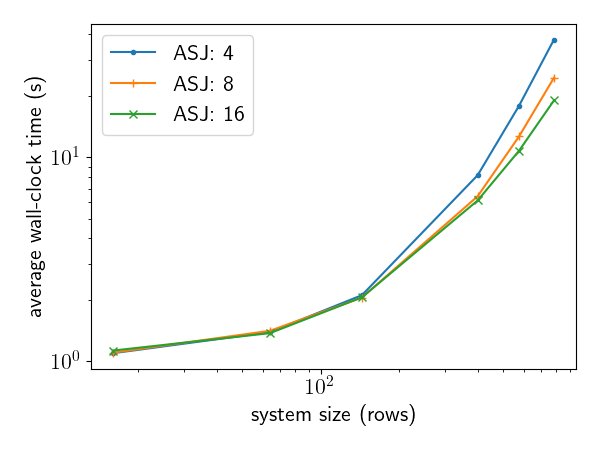
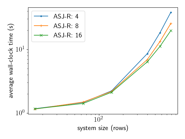
Figure 2: Scaling of ensemble average wall-clock time with respect to condition number for various Poisson matrices, ranging in row counts from 16 to 784, and various numbers of Skywing agents. The scaling for both ASJ (left) and ASJ-R (right) exhibit the expected reduction in wall-clock time with more agents once the system size is sufficiently large.

We see that once system size is sufficiently large, around more than $200$ rows, the computational cost of computing the iterates becomes greater than the cost of communicating the iterates between agents so that the target numerical solution is attained is less time with more agents. We also verify that the ASJ-R timing results are nearly identical to ASJ, which is expected in the absence of any data corruption. Note that the wall-clock time results do include the $1$ second “convergence duration” described at the end of Section 3.

4.3 Path Length Rejection Variant with Data Corruption

We evaluate the resilience of the ASJ rejection variant (ASJ-R) to both natural and malevolent corruption, as defined in Section 2.1 and Section 2.2, respectively. All numerical studies consider the Poisson problem (9) on a mesh with $20\times 20$ interior points ($\ell=20$) distributed evenly over $16$ Skywing agents. We note that our focus is on the convergence of ASJ and ASJ-R in the presence of failures and not necessarily on the scalability of the algorithms. There are indeed more scalable, powerful linear solvers than Jacobi: our work is meant as the initial step towards corruption detection methods that enable those linear solvers to circumvent unreliability in emerging computing environments.

Natural Data Corruption

Our first investigation introduces bit flips to communicated data, similar to the studies performed by Anzt et al. in [2]. We aim to assess the impact of the probability $p$ of a bit flip on the convergence of both ASJ and ASJ-R. As discussed in Section 2.1, corruption is applied at each iteration and on every agent with probability $p$ to all communicated data. The elements of $\mathbf{x}_{i}^{\kappa}$ in both ASJ and ASJ-R are stored as ieee 754 double floating point numbers, whereas the values of the approximate shortest path length $\tilde{s}_{i}(t)$ in ASJ-R are stored as signed integers. If a given double floating point value is chosen to be corrupted, a bit index out of a given subset of its $64$ bit representation is randomly chosen to be flipped. If a given signed integer value is chosen to be corrupted, a bit index out of any of its $32$ bit representation is randomly chosen to be flipped.

For our first study, we fix the probability of a bit flip in a given communicated value to be $p=0.01$. Following Anzt et al. [2], we investigate the following double floating point subsets: the lower mantissa $\textsc{ie}^{3}({[0{-}25]})$, the upper mantissa $\textsc{ie}^{3}({[26{-}51]})$, the exponent $\textsc{ie}^{3}({[52{-}62]})$, and the sign bit $\textsc{ie}^{3}({63})$. We start with the lower mantissa subset $\textsc{ie}^{3}({[0{-}25]})$, which leads to floating point value corruption ranging from $1/2^{52}\approx 10^{-16}$ to $1/2^{27}\approx 10^{-8}$ relative to the original values. Figure 3 shows the convergence behavior for ASJ and ASJ-R.

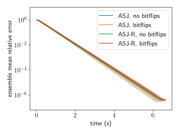
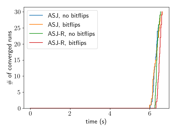
Figure 3: Ensemble convergence of ASJ and ASJ-R with bit flip probability $p=0.01$, with double floating point flips limited to the lower mantissa $\textsc{ie}^{3}({[0{-}25]})$. Convergence is achieved in all ASJ and ASJ-R runs, with times to solution comparable to the respective baseline (no bit flip) values.

For both ASJ and ASJ-R, all runs in the respective bit flip ensemble converge with times to solution that are approximately the same as those of the respective baseline (no bit flip) ensembles. The indifference of the ASJ convergence behavior to lower-mantissa flips is consistent with Anzt et al. [2], where it was found that ASJ convergence behavior is not affected by such bit flips until the relative residual norm is reduced to a very small value. The indifference is due to the corruption caused by lower-mantissa flips being too small to significantly affect the iteration evolution to the tolerance $\epsilon=10^{-5}$, as relaxation methods are inherently robust to small amounts of corruption.

To introduce larger corruption, we now investigate the sign bit $\textsc{ie}^{3}({63})$ subset, which leads to floating point value corruption of $2$ relative to the original values. Figure 4 shows the convergence behavior for ASJ and ASJ-R.

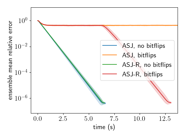
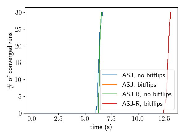
Figure 4: Ensemble convergence of ASJ and ASJ-R with bit flip probability $p=0.01$, with double floating point flips limited to the sign bit $\textsc{ie}^{3}({63})$. Convergence is lost for all of the ASJ runs and achieved for all ASJ-R runs, albeit with longer times to solution.

For ASJ, the effect of the more significant corruption from sign bit flips is evident as the solution error of all ASJ runs decreases at first but then stagnates at a level well above the convergence tolerance, consistent with the findings of [2]. The introduction of the rejection criterion in ASJ-R, based on (5), restores convergence in all of the runs, albeit with a longer time to solution. Whereas the convergence of the baseline ASJ-R ensemble is obtained for all runs around $6.5$s, the time to convergence increases to around $12.5$s for ASJ-R runs with bit flips. This increased time to solution is explained by the presence of a stagnation period from around $t=0.5$s until around $t=7$s for all ASJ-R runs with bit flips. Given that the ASJ-R error during this stagnation period coincides with the stagnated ASJ error, it can be inferred that the value of the approximate shortest path length $\tilde{s}_{i}(t)$ in (5) during the stagnation period is not yet large enough for ASJ-R to reject the corruption. Figure 5 shows the value of the approximate shortest path length for the two agents receiving updates from the corrupted agent.

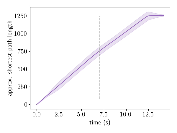
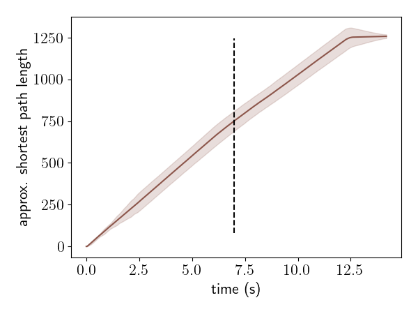
Figure 5: Approximate shortest path length $\tilde{s}_{i}(t)$ used by ASJ-R algorithm with bit flip probability $p=0.01$, with double floating point flips limited to the sign bit $\textsc{ie}^{3}({63})$ (left: $i=7$, right: $i=9$). The approximate shortest path length reaches $750$ at around the time the stagnation period ends in Figure 4 (denoted by dashed black line).

The values of $\tilde{s}_{7}(t)$ and $\tilde{s}_{9}(t)$ grow roughly linearly with time until around the end of the stagnation period $t=7$s. Around $t=7$s, the value of $\tilde{s}_{i}(t)$ is large enough ($\approx 750$) to start rejecting data containing bit flips so that all $30$ runs can resume converging. The values of $\tilde{s}_{7}(t)$ and $\tilde{s}_{9}(t)$ continue to grow linearly after $t=7s$, albeit at a slightly slower rate overall than $t<7$s due to the rejections.

To introduce corruption with a relative magnitude between the sign bit and lower mantissa subsets, we now investigate the upper mantissa $\textsc{ie}^{3}({[26{-}51]})$ subset, which leads to floating point value corruption ranging from $1/2^{26}\approx 10^{-7}$ to $1/2$ relative to the original values. Figure 6 shows convergence behavior for ASJ and ASJ-R.

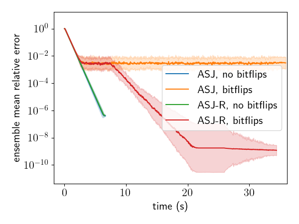
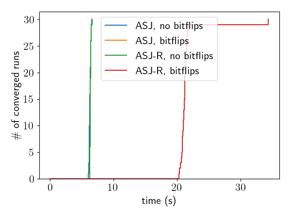
Figure 6: Ensemble convergence of ASJ and ASJ-R with bit flip probability $p=0.01$, with double floating point flips limited to the upper mantissa $\textsc{ie}^{3}({[26{-}51]})$. Convergence is lost for all of the ASJ runs and achieved for all ASJ-R runs, with the times to solution of the convergent runs being longer, and more variable than that of sign bit flips (Figure 4).

For ASJ, the corruption from upper-mantissa flips is still large enough to prevent convergence in all runs, with the solution error stagnating at a level above tolerance but lower than with sign bit flips, consistent with the smaller magnitude value changes and with the findings of [2]. For ASJ-R, convergence is achieved in all runs with a time to solution around $20$s or $21$s for most runs, with one run taking around $33$s or $34$s. Note the presence of a stagnation period followed by a return to convergence behavior seen with sign bit flips, although the stagnation period now lasts until around $t=7.5$s and the time to solution is longer and more variable than the sign bit results. Figure 7 shows the value of the $\tilde{s}_{i}(t)$ for the two agents receiving updates from the corrupted agent.

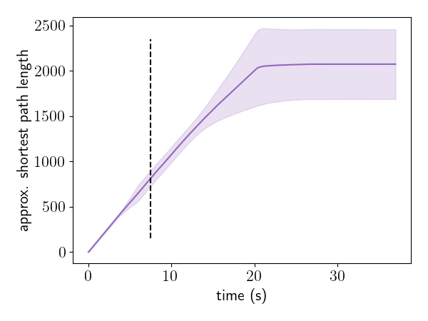
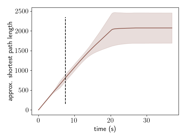
Figure 7: Approximate shortest path length $\tilde{s}_{i}(t)$ used by ASJ-R algorithm with bit flip probability $p=1\%$, with double float point flips limited to the sign bit $\textsc{ie}^{3}({[26{-}51]})$ (left: $i=7$, right: $i=9$). The approximate shortest path length reaches $750$ at around the time the stagnation period ends in Figure 6 (denoted by dashed black line).

The values of $\tilde{s}_{7}(t)$ and $\tilde{s}_{9}(t)$ again grow roughly linearly with time until reaching a value of around $750$ at $t=7.5$s. To understand why corruption of smaller relative magnitude both requires larger $\tilde{s}_{i}(t)$ values to end stagnation and causes slower convergence, it is important to note that as $\tilde{s}_{i}(t)$ grows, there is always corruption of a certain magnitude that will not be rejected. Whether or not that magnitude at time $t$ happens to be significant, with respect to continuing to reduce the error at time $t$, likely introduces the variability seen for $t>7.5$s in both the convergence rate and growth of $\tilde{s}_{i}(t)$. It is worth noting that Anzt et al. [2] also see a slower rate of convergence for synchronous Jacobi with bit flips for likely the same reason: there is always corruption of a certain magnitude that will not be rejected by the contraction mapping rejection criterion used in their work, albeit the static threshold in their criterion avoids the stagnation period.

The last subset to investigate is the exponent subset $\textsc{ie}^{3}({[52{-}62]})$, which leads to floating point value changes ranging from $1$ to $2^{1023}-1\approx 10^{308}$ relative to the original values. Figure 8 shows the convergence behavior for ASJ and ASJ-R.

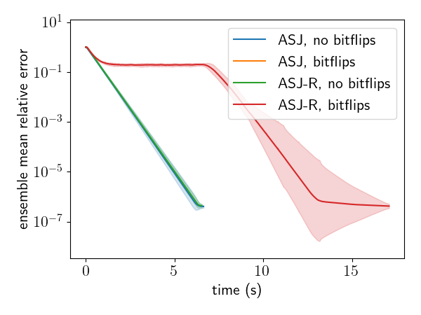
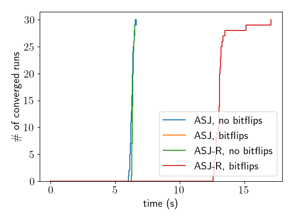
Figure 8: Ensemble convergence of ASJ and ASJ-R with bit flip probability $p=0.01$, with double floating point flips limited to the exponent $\textsc{ie}^{3}({[52{-}62]})$. Convergence is lost for all of the ASJ runs and achieved for all ASJ-R runs, with the times to solution being mostly comparable to that of sign bit flips (Figure 4)

For ASJ, the corruption from exponent flips is large enough that all runs result in solution iterates containing non-finite (i.e., ieee 754 NaN) values after just a few iterations, which is consistent with the findings of [2]. For ASJ-R, convergence is achieved in all runs with a time to solution similar to that of the sign bit flips: around $12.5$s for most runs, with a few runs taking up to $17$s to converge. The behavior is consistent with the interpretation of the convergent sign bit or upper mantissa flip results: after a stagnation period, the bit flip corruptions large enough to prevent convergence are rejected as $\tilde{s}_{i}(t)$ increases. It is interesting to note that the error level of the stagnation period is smaller with exponent flips than with sign bit flips, despite the ability of exponent flips to result in much larger changes relative to the original values (e.g., $10^{308}$ vs $2$). This effect is explained by how even $\tilde{s}_{i}(t)=0$ in (5) will reject exponent flips that result in value changes much larger than those that of sign bit flips.

With an understanding of how ASJ and ASJ-R perform on bit flips with probability $p=0.01$ in subsets of the floating point double, we now investigate flipping any of $64$ bits with probability $p$ values of $0.0025$, $0.005$, $0.01$, $0.015$, $0.02$, and $0.04$. For ASJ, all of the runs in any ensemble corresponding to $p>0$ quickly saw NaN values in the solution iterates. Noting similar divergence to NaN values in Figure 8, one can infer that, even with bit flip probability as low as $p=0.0025$, the ASJ runs quickly experience the occurrence of one or more exponent bit flips. For ASJ-R, the convergence behavior is shown in Figure 9.

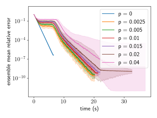
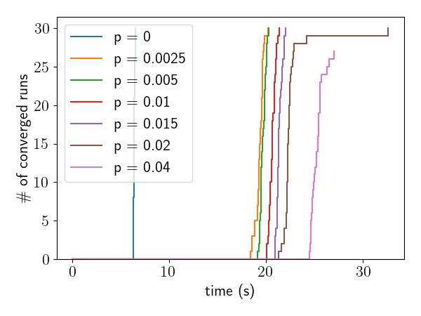
Figure 9: Ensemble convergence of ASJ-R with bit flip corruption probabilities ranging from $p=0$ to $p=0.04$, with double floating point flips in any of the $64$ bits. Convergence is lost for all of the ASJ runs and achieved for all but $3$ ASJ-R runs, with the stagnation period duration, the stagnation period error value, the time to solution, and the time to solution variability all increasing with increasing $p$.

Almost all ensembles resulted in all runs converging, with the exception of $p=0.04$ where $27$ of $30$ runs converged. For each value of $p>0$, the convergent runs experience a stagnation period followed by convergence with a variable time to solution that is longer than with $p=0$. It is worth noting that the error value and duration of the stagnation period, the time to solution, and the variability of the time to solution all increase with increasing $p$. Recall that the subset studies attributed the existence of the stagnation period to large corruption that avoided rejection until $\tilde{s}_{i}(t)$ increased to a certain value. The studies also showed that very large corruption is likely always rejected, i.e., even at $\tilde{s}_{i}(t)=0$, resulting in the largest stagnation period error value being produced by corruption around that of the sign bit flip. Thus, a longer stagnation period at a larger error value for larger $p$ is explained by the increased probability of bit flips that cause corruption around that of the sign bit before $\tilde{s}_{i}(t)$ reaches the value necessary to resume convergence. That increasing $p$ leads to longer and more variable time to solution is explained by the increased probability of bit flips that cause corruption that is large enough to delay convergence but small enough to avoid rejection by the increasing $\tilde{s}_{i}(t)$. All in all, the ASJ-R algorithm has a very high probability of converging even when a large number of bit flips occur, e.g., $p=0.04$ of communicated data are corrupted at each iteration.

Malevolent Data Corruption

Our second investigation introduces malevolent manipulation of stored data, as defined in Section 2.2. We aim to assess the impact of the recovery time $\omega_{r}$ and mean manipulation offset $\delta$ on the convergence of both ASJ and ASJ-R. As described in Section 2.2, while agent $i$ is in a degraded state, every element of $\mathbf{x}_{i}^{\kappa}$ is manipulated by an additive offset sampled from a normal distribution with mean $\delta$ and standard deviation $\tfrac{1}{2}\delta$. The time-to-failure $\omega_{f}$ for all comprised agents is chosen by considering both the convergence duration in the stopping criterion (6), which is $1$s and the typical time the ASJ method takes to converge in the absence of data corruption, which is approximately $6$s or $7$s. Note that a time-to-failure less than the convergence duration ($\omega_{f}<1$s) will effectively guarantee a loss of convergence, while a time-to-failure greater than the time it takes to converge in the absence of data corruption ($\omega_{f}>7$s) will effectively guarantee convergence. Considering these limits, we choose to compromise agent $8$ and investigate two time-to-failure values: $\omega_{f}=5$s and $\omega_{f}=2.5$s. Given those time-to-failure values, we chose to study recovery times $\omega_{r}$ selected from $0.2$s, $0.4$s, and $0.6$s, and offset magnitudes $\delta$ selected from $0.1$, $0.2$, $0.3$, $0.4$, and $0.5$.

We first study corruption with time-to-failure $\omega_{f}=5$s. Figure 10 shows the convergence behavior of ASJ both for various $\omega_{r}$ with fixed $\delta=0.2$ and for fixed $\omega_{r}=0.2$s with various $\delta$.

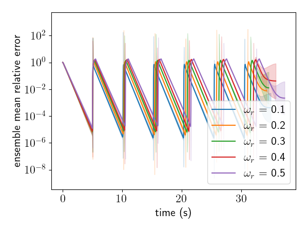
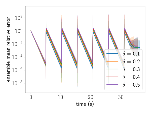
Figure 10: Ensemble convergence of ASJ with malevolent corruption with time-to-failure $\omega_{f}=5$s, various recovery times $\omega_{r}$, and various offset magnitudes $\delta$ (left: various $\omega_{r}$ values and $\delta=0.2$, right: $\omega_{r}=0.2$s and various $\delta$ values). Convergence is not obtained for any of the runs.

All of the ASJ runs fail to converge for the recovery times and offset magnitudes explored. The effect of the corruption is seen around $5$s as the solution error becomes small enough to begin the convergence duration (see end of Section 3) but then rapidly increases due to the corruption on agent $8$ that quickly propagates to other agents. The error increases to a peak that coincides with agent $8$ returning to a normal state, after which the error does decrease until the next rapid increase when agent $8$ is again degraded. As one might expect, increasing either the recovery time $\omega_{r}$ or the offset magnitude $\delta$ increases the amount the error jumps when agent $8$ is compromised. Note that Figure 10 does include a period of increasing ensemble variability for large $t$: this merely represents the variability in when the $16$ agents each determine that the maximum number of iterations has been reached. Excluding that period, one sees the expected overall increasing error trend expected from unmitigated periodic corruption.

Figure 11 shows the convergence behavior of ASJ-R for recovery time $\omega_{r}=0.2$s and various offset magnitudes $\delta$.

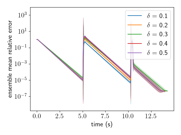
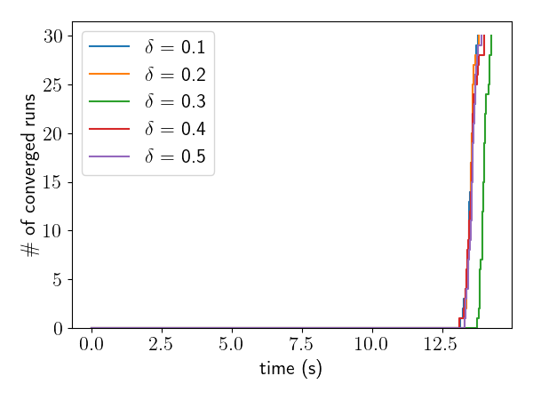
Figure 11: Ensemble convergence of ASJ-R with malevolent corruption with time-to-failure $\omega_{f}=5$s, recovery time $\omega_{r}=0.2$s, and various offset magnitudes $\delta$. Convergence is achieved for all runs, with the time to solution being comparable to that of bit flip (Figure 4) and exponent flip (Figure 8) corruption.

All of the ASJ-R runs converge with a time to solution around $13$s. Note the two periods of degraded state in agent $8$, which total $0.4$s with $\omega_{r}=0.2$s, do not account for the entire increase in time to solution (recall ASJ-R only required $6$s or $7$s without corruption). The remainder of the increase in time to solution is explained by the same mechanism that causes the stagnation period with bit flip corruption: the value of $\tilde{s}_{i}(t)$ in (5) is not large enough at $t=5$s to prevent the malevolent corruption on the degraded agent $8$ from spreading to other agents. Note that the increase in error around $t=5$s appears very similar to the corresponding ASJ results at $t=5$s in Figure 12. By the time agent $8$ becomes degraded the second time, i.e., $t=10s$, the value of $\tilde{s}_{i}(t)$ is large enough to prevent the corruption from spreading. To see this, note the error around $t=10$s jumps to a certain level, due to the corruption of values in $\mathbf{x}_{8}^{\kappa}$, but then remains constant for the duration of the degraded state instead of growing, implying the values of $\mathbf{x}_{i}^{\kappa}$ for $i\neq 8$ are not affected. Once agent $8$ returns to a normal state the second time, the corrupted values on agent $8$ are iteratively corrected by updates from the unaffected agents, and the solution iterates converge before agent $8$ enters a third degraded state. Figure 12 shows the convergence behavior of ASJ-R for various recovery times $\omega_{r}$ with offset magnitude $\delta=0.2$.

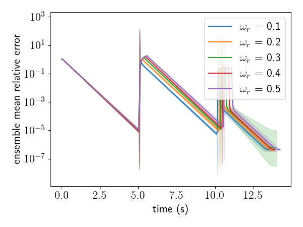
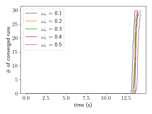
Figure 12: Ensemble convergence of ASJ-R with malevolent corruption with time-to-failure $\omega_{f}=5$s, various recovery times $\omega_{r}$, and offset magnitude $\delta=0.2$. Convergence is achieved for all runs, with the time to solution increasing proportional to the increases in $\omega_{r}$.

All ASJ-R runs are similarly able to converge by preventing the spread of the corruption on agent $8$ once $\tilde{s}_{i}(t)$ is large enough (i.e., after the first degraded state), with the time to solution growing proportional to the increases in $\omega_{r}$.

Given that ASJ-R was able to restore convergence in all runs with time-to-failure $\omega_{f}=5$s, we now study the more difficult case of $\omega_{f}=2.5$s. The shorter time-to-failure is more difficult because the $\omega_{f}=5$s results indicate that $\tilde{s}_{i}(t)$ is not large enough to reject malevolent corruption until at least $t=5.5s$, i.e., that agent $8$ will go through two unmitigated degraded states. Figure 13 shows the convergence behavior of ASJ-R for recovery time $\omega_{r}=0.2$s with various offset magnitudes $\delta$.

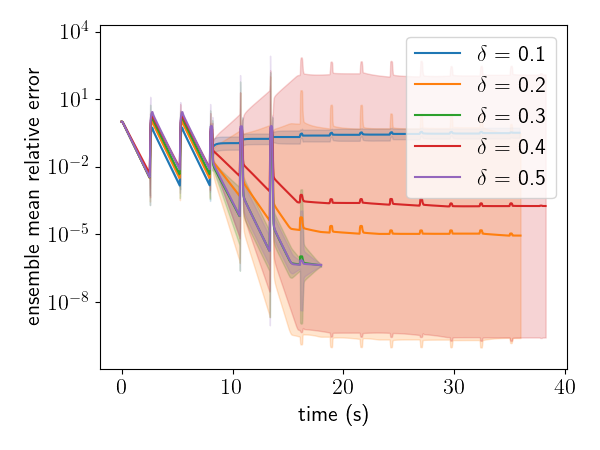
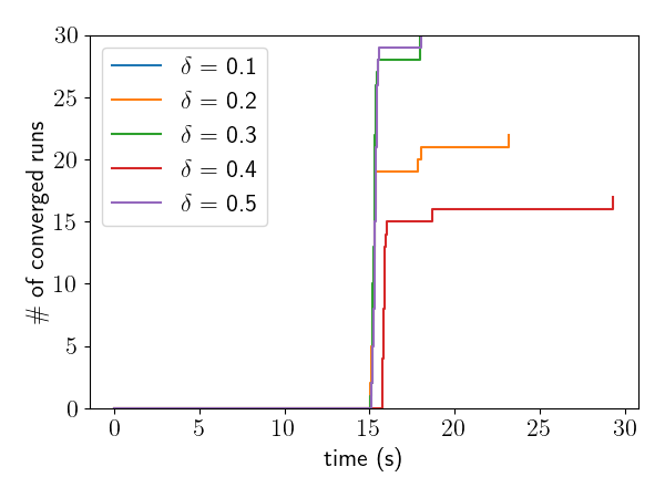
Figure 13: Ensemble convergence of ASJ-R with malevolent data corruption with time-to-failure $\omega_{f}=2.5$s, recovery time $\omega_{r}=0.2$s, and various offset magnitudes. The likelihood of convergence is highly variable and seemingly dependent on whether or not the corruption from the third degraded state is mitigated.

The shorter time-to-failure $\omega_{f}=2.5$ leads to highly variable results, with the number of ASJ-R runs that converge ranging from $0$ for $\delta=0.1$ to all $30$ for $\delta=0.5$. Note that for all runs, the shorter time-to-failure does indeed result in two rounds of unmitigated corruption as $\tilde{s}_{i}(t)$ is not yet large enough for (5) to reject the corrupted updates. Whether or not $\tilde{s}_{i}(t)$ is large enough around $t=7.9$s to reject the corruption from the third time agent $8$ enters a degraded state appears to determine whether the ASJ-R will eventually converge or not. The failure of convergence for those runs that do not mitigate the third degraded state in agent $8$ results from that all agents eventually begin rejecting all updates from agent $8$, including valid updates that now include large changes required to advance the corrupted $\mathbf{x}_{8}^{\kappa}$ back towards the solution, leading to a persistent stagnation in the error. Figure 14 shows the convergence behavior of ASJ-R for various recovery times $\omega_{r}$ with offset magnitude $\delta=0.2$.

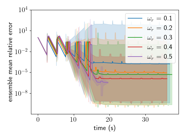
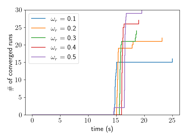
Figure 14: Ensemble convergence of ASJ-R with malevolent data corruption with time-to-failure $\omega_{f}=2.5$s, various recovery times $\omega_{r}$, and offset magnitude $\delta=0.2$. The likelihood of convergence is proportional to the recovery time, i.e., the longer the recovery time, the more likely ASJ-R will converge.

One might predict that shorter recovery times, which mean less time that agent $8$ is corrupted per degraded state, would result in more convergent runs. The ASJ-R runs instead exhibit the opposite behavior: the shorter the recovery time, the fewer runs converge. This is understood by noting that shorter recovery times mean less time for $\tilde{s}_{i}(t)$ to grow before agent $8$ enters another degraded state. Thus, while the longer recovery times mean more corrupted iterations per degraded state, they also allow for $\tilde{s}_{i}(t)$ to grow enough to mitigate those corrupted iterations by the third degraded state and achieve convergence.

4.4 Path-Length Rejection Considerations

Recall that the ASJ-R rejection criterion (5) is developed on theory that uses the exact shortest path length $s_{i}(t)$, which is typically not available to the agents and therefore replaced by an approximation $\tilde{s}_{i}(t)$. We saw in Section 4.3 that whether $\tilde{s}_{i}(t)$ in (5) is sufficiently large to reject significant corruption at a given time $t$ has a profound impact on the convergence of ASJ-R, ranging from a temporary stagnation period that results in a longer time-to-solution to persistent stagnation that prevents convergence all together. While a more rigorous study is warranted for future work, the values of $\tilde{s}_{i}(t)$ as defined in Algorithm 1 are found to consistently underestimate the values of $s_{i}(t)$ for runs that were anecdotally selected. As such, one might both significantly reduce the ASJ-R time-to-solution and increase the likelihood of convergence in the presence of corruption with a more accurate approximate shortest path length $\tilde{s}_{i}(t)$ that reduces or eliminates the stagnation issues in Section 4.3.

Another consideration for the practical use of ASJ-R is the dependence of the rejection criterion (5) on singular values. For the system sizes considered in Section 4.3, the values of $\sigma_{\text{min}}(A)\approx 0.0447$ and $\sigma_{\text{max}}(M)\approx 0.989$ are relative cheap to compute locally on each agent; however, one might want to apply ASJ-R to large systems or to systems where agents do not have access to all rows of $A$. As such, the malevolent corruption study with time-to-failure $\omega_{f}=5$s, recovery time $\omega_{r}=0.2$s, and offset magnitude $\delta=0.2$ is repeated for ASJ-R but with either $\sigma_{\text{min}}(A)$ or $\sigma_{\text{max}}(M)$ replaced in (5) by approximate values. Figure 15 shows the convergence behavior of ASJ-R with $\sigma_{\text{min}}(A)$ replaced by the numerically computed value scaled by one of $10^{-4}$, $10^{-2}$, $1$, $10^{2}$, or $10^{4}$.

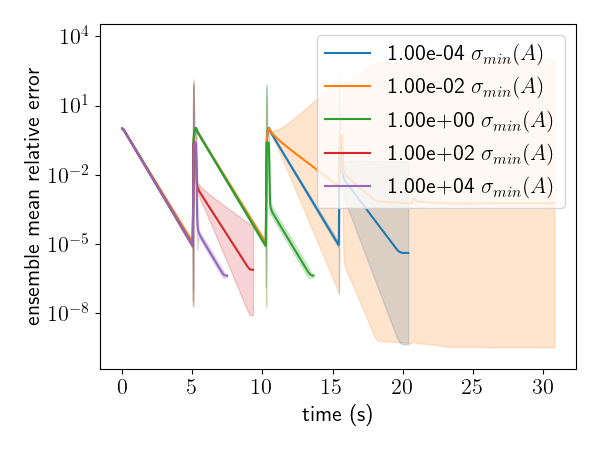
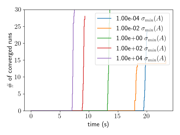
Figure 15: Ensemble convergence for ASJ-R with malevolent data corruption using various scaled values of $\sigma_{\text{min}}(A)$ in the rejection criterion (5). Convergence in attained in almost all runs for all scaling factors except $10^{-4}$ scaling, with time-to-solution values improving for larger scaling factors.

The convergence behavior suggests that ASJ-R is robust to the use of approximated values for $\sigma_{\text{min}}(A)$ in (5), with the larger scaled values resulting in more reliable convergence, i.e., $28$ and $30$ of $30$ runs converging for scaling values of $10^{2}$ and $10^{4}$, respectively, and $24$ and $15$ runs converging for scaling values of $10^{-2}$ and $10^{-4}$, respectively. A second important result is that the time-to-solution values for the convergent runs decrease as the scaling factor increases. These two results are explained by how a larger value to replace $\sigma_{\text{min}}(A)$ leads to a tighter bound in (5) that likely offsets some of the effect of the underestimated shortest path length and, therefore, results in less corrupted values avoiding rejection. Figure 16 shows the convergence behavior of ASJ-R with $\sigma_{\text{max}}(M)$ replaced by the numerically computed value scaled by one of $0.98$, $0.99$, $0$, $1.01$, or $1.02$.

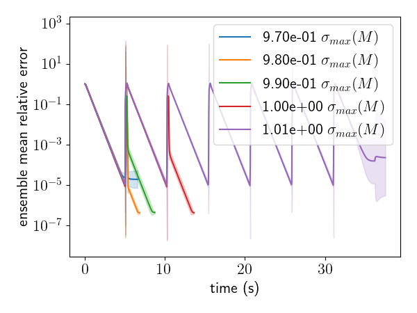
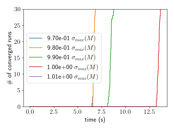
Figure 16: Ensemble convergence for ASJ-R with malevolent data corruption using various perturbed values of $\sigma_{\text{max}}(M)$ in the rejection criterion (5). Convergence is not attained for any ensemble runs with scaling factors $1\pm 0.2$ and is attained for all ensemble runs with scaling factors $1\pm 0.1$, with optimal time-to-solution for $0.98$ scaling factor.

The convergence behavior suggests that ASJ-R is much less robust to the use of approximated values for $\sigma_{\text{min}}(M)$ as the ensembles quickly go from all the runs converging with scaling factor $1\pm 0.01$ to all runs failing to converge with scaling factor $1\pm 0.02$. That the time-to-solution for a perturbation of $0.99$ is shorter than when the true value of $\sigma_{\text{max}}(M)$ is used, is likely due to the former leading to a tighter bound in (5) that offsets the underestimated shortest path length and, again, results in less corrupted values avoiding rejection. It is worth noting that the results from Figure 15 and Figure 16 both support the hypothesis that a better shortest path length approximation $\tilde{s}_{i}(t)$ will significantly improve ASJ-R convergence.

5 Conclusions

In this paper, we have introduced a fault-tolerant Asynchronous Jacobi (ASJ) variant that leverages ASJ convergence theory by Hook and Dingle [9] to provide resilience to data corruption. The resulting ASJ Rejection Variant (ASJ-R) strategy rejects solution approximations from neighbor nodes if the distance between two successive approximations violates an analytic bound. Following the work of Anzt et al. [2], we studied the resilience of ASJ and ASJ-R to corruption in communicated data due to bit flips in various parts of the ieee 754 floating point representation. We first confirmed both ASJ and ASJ-R reliably converge when the corruption is very small relative to the convergence tolerance. For larger corruption, we found that ASJ-R can reliably converge in various scenarios where ASJ failed to converge at all. We attribute the convergence of ASJ-R to the rejection criterion reliably rejecting corruption once the associated approximation to the shortest path length increases to a particular value, which depends on the corruption size. While the corruption that is not rejected until the shortest path length is sufficiently large does cause the error to temporarily stagnate, once the approximation is large enough to reject corruption, the remaining iterations that do not involve corruption then drive the error down to the specified tolerance. It is worth noting that a longer time to solution is observed when corruption is present due to the combination of stagnation period followed by properly rejected iterations that do not contribute to decreasing the error, with the longest time to solution occurring when the corruption is large enough to affect the convergence yet small enough to require a larger shortest path length approximation for rejection.

We also studied the resilience of ASJ and ASJ-R to the corruption of stored data, where the values are perturbed by a given amount for periodic windows of time. Whereas ASJ failed to converge in all the scenarios tested, ASJ-R reliably converged so long as there was sufficient time between the corruption windows to allow the shortest path length approximation to become sufficiently large. We also studied the convergence of ASJ-R on stored data corruption when approximate values are used for the two singular values in the rejection criterion. We found the results to be more sensitive to the maximum singular value of the iteration matrix and less sensitive to the minimum singular value of the linear system matrix, which is promising as the latter is typically more difficult to obtain. Skewing of either singular values in the direction that tightened the rejection criterion bound were found to more likely maintain, or even improve, convergence behavior than skewing that loosened the bound. Overall, the ASJ-R strategy restored convergence lost by ASJ in the presence of corruption in a variety of scenarios, with the convergence of ASJ-R likely improved by future work developing a better approximation to the shortest path length or dynamic adjustments to the rejection criterion bound.

References

- [1] IEEE standard for floating-point arithmetic, IEEE Std 754-2019 (Revision of IEEE 754-2008), (2019), pp. 1–84, https://doi.org/10.1109/IEEESTD.2019.8766229.
- [2] H. Anzt, J. Dongarra, and E. S. Quintana-Ortí, Tuning stationary iterative solvers for fault resilience, in Proceedings of the 6th Workshop on Latest Advances in Scalable Algorithms for Large-Scale Systems, ScalA ’15, New York, NY, USA, 2015, Association for Computing Machinery, https://doi.org/10.1145/2832080.2832081.
- [3] Apache Software Foundation, Hadoop, 2021, https://hadoop.apache.org.
- [4] Apache Software Foundation, Spark, 2021, https://spark.apache.org.
- [5] R. Canal, C. Hernandez, R. Tornero, A. Cilardo, G. Massari, F. Reghenzani, W. Fornaciari, M. Zapater, D. Atienza, A. Oleksiak, W. Piątek, and J. Abella, Predictive reliability and fault management in exascale systems: State of the art and perspectives, ACM Comput. Surv., 53 (2020), https://doi.org/10.1145/3403956.
- [6] D. Chazan and W. Miranker, Chaotic relaxation, Linear Algebra and its Applications, 2 (1969), pp. 199–222, https://doi.org/https://doi.org/10.1016/0024-3795(69)90028-7.
- [7] Z. Chen, Online-ABFT: An online algorithm based fault tolerance scheme for soft error detection in iterative methods, in Proceedings of the 18th ACM SIGPLAN Symposium on Principles and Practice of Parallel Programming, PPoPP ’13, New York, NY, USA, 2013, Association for Computing Machinery, p. 167–176, https://doi.org/10.1145/2442516.2442533.
- [8] A. Frommer and D. B. Szyld, On asynchronous iterations, Journal of Computational and Applied Mathematics, 123 (2000), pp. 201–216, https://doi.org/10.1016/S0377-0427(00)00409-X. Numerical Analysis 2000. Vol. III: Linear Algebra.
- [9] J. Hook and N. Dingle, Performance analysis of asynchronous parallel Jacobi, Numerical Algorithms, 77 (2018), pp. 831–866, https://doi.org/10.1007/s11075-017-0342-9.
- [10] Q. Li, B. Kailkhura, R. Goldhahn, P. Ray, and P. K. Varshney, Robust decentralized learning using admm with unreliable agents, 2018, https://arxiv.org/abs/1710.05241.
- [11] X. Liang, J. Chen, D. Tao, S. Li, P. Wu, H. Li, K. Ouyang, Y. Liu, F. Song, and Z. Chen, Correcting soft errors online in fast Fourier transform, in Proceedings of the International Conference for High Performance Computing, Networking, Storage and Analysis, SC ’17, New York, NY, USA, 2017, Association for Computing Machinery, https://doi.org/10.1145/3126908.3126915.
- [12] M. A. Mukwevho and T. Celik, Toward a smart cloud: A review of fault-tolerance methods in cloud systems, IEEE Transactions on Services Computing, 14 (2021), pp. 589–605, https://doi.org/10.1109/TSC.2018.2816644.
- [13] A. Olshevsky, I. C. Paschalidis, and A. Spiridonoff, Fully asynchronous push-sum with growing intercommunication intervals, in 2018 Annual American Control Conference (ACC), June 2018, pp. 591–596, https://doi.org/10.23919/ACC.2018.8431414. ISSN: 2378-5861.
- [14] C. Ponce, K. Harter, A. Fox, and C. Vogl, Skywing, 2022, https://doi.org/10.11578/dc.20221110.2.
- [15] J. Wolfson-Pou and E. Chow, Convergence models and surprising results for the asynchronous Jacobi method, 2018 IEEE International Parallel and Distributed Processing Symposium (IPDPS), (2018), pp. 940–949.
- [16] P. Wu, C. Ding, L. Chen, F. Gao, T. Davies, C. Karlsson, and Z. Chen, Fault tolerant matrix-matrix multiplication: Correcting soft errors on-line, in Proceedings of the Second Workshop on Scalable Algorithms for Large-Scale Systems, ScalA ’11, New York, NY, USA, 2011, Association for Computing Machinery, p. 25–28, https://doi.org/10.1145/2133173.2133185.