Evolution of black holes through a nonsingular cosmological bounce

Abstract

We study the classical dynamics of black holes during a nonsingular cosmological bounce. Taking a simple model of a nonsingular bouncing cosmology driven by the combination of a ghost and ordinary scalar field, we use nonlinear evolutions of the Einstein equations to follow rotating and non-rotating black holes of different sizes through the bounce. The violation of the null energy condition allows for a shrinking black hole event horizon and we find that for sufficiently large black holes (relative to the minimum Hubble radius) the black hole apparent horizon can disappear during the contraction phase. Despite this, we show that most of the local cosmological evolution remains largely unaffected by the presence of the black hole. We find that, independently of the black hole’s initial mass, the black hole’s event horizon persists throughout the bounce, and the late time dynamics consists of an expanding universe with a black hole of mass comparable to its initial value.

1 Introduction

A proposed alternative to cosmic inflation is the idea that the universe underwent a bounce: a transition from a stage of contraction to expansion [1, 2, 3, 4, 5]. In a singular bounce, the universe passes through a classical singularity where the cosmological scale factor becomes small, curvature invariants blow up, and quantum gravity effects presumably become highly relevant to determining the future dynamics of the universe [6, 7, 8, 9]. An alternative, which we focus on here, is a nonsingular bounce. For such cosmologies, so long as the spacetime curvature does not become Planckian, there is the possibility that quantum gravity effects could be subdominant to classical effects, in which case one may be able to describe the dynamics of the bounce using classical physics. Nonsingular bouncing cosmologies require violating the null convergence condition (NCC), which states that for all null vectors $k^{\mu}$, $R_{\mu\nu}k^{\mu}k^{\nu}\geq 0$ [10, 11, 4, 12, 5]. In Einstein gravity, the NCC is equivalent to the null energy condition which is satisfied by most standard classical field theories [12]. Nonsingular bouncing cosmologies hence require non-standard matter terms, or modifications to Einstein gravity, for example, Horndeski theories including ghost condensation [13, 14] or (cubic) Galileon/Horndeski models [15, 16, 17, 18, 19, 20]. While perturbative studies of these theories suggest they may be free of ghost or gradient instabilities [16, 19], less is known about which models will remain (strongly) hyperbolic through a bounce, when the solution is presumably not in the weakly coupled regime [21, 22, 23]

An important open question is what happens in bouncing cosmologies in the inhomogeneous and non-perturbative regime. While there are several analytical and numerical studies of the dynamics of bouncing cosmologies during their contraction phase [25, 26, 27, 28], there are relatively few studies of the dynamics of the bounce [29, 30, 31, 32, 19], and none that consider the dynamics of black holes beyond the restriction to spherical symmetry [33]. Previous studies of black hole–cosmological bounces have either constructed initial data for black hole bouncing solutions [34], worked in a perturbative limit [35, 36, 37, 38], or made use of analytic solutions (e.g. generalizations of the McVittie solutions [39, 40, 41]), that are limited by the fact that the metric evolution is prescribed ad-hoc, and from that the implied matter type and evolution is derived. The question of what happens to a black hole in a nonsingular cosmological bounce is particular salient for several reasons. On the one hand, the bounce necessarily requires a violation of the assumptions made in black hole singularity theorems and results on black hole horizons (namely the NCC) [42], so there is a question of whether the black hole will survive the bounce, or if the bounce mechanism will also reverse gravitational collapse, and if this will possibly lead to a naked singularity. On the other hand, one might also worry what the backreaction of the black hole’s gravity will be on the bounce in the neighbourhood of the black hole. An extreme scenario would be if the bounce failed to happen in the vicinity of the black hole, possibly leading to a patch of contraction that grows into the expanding spacetime, as happens, e.g., in scenarios where the Higgs boson is destabilized during inflation, and goes to its true vacuum at negative energy densities [43, 44].

Here, we address these questions by studying the nonlinear dynamics and evolution of black holes in a particular nonsingular bouncing cosmology (details of which are described below). Black holes can be expected to form during the contraction of matter and radiation dominated universes [45, 36, 46], and will generally be present from previous eras in cyclic cosmologies [47, 48]. However, it is common to invoke a smoothing phase during contraction (e.g. ekpyrosis [49, 47, 50]), and argue that Hubble patches containing a black hole will be rare. Regardless, we view our work as serving two main purposes: (1) to study the dynamics and robustness of a nonsingular bouncing model when a very large perturbation, namely a black hole, is introduced, and (2) to explore the dynamics of the black hole and cosmological horizons during the bounce.

To avoid the difficulties related to finding a motivated theory that can give rise to bouncing solutions while also having well-posed evolution equations in the inhomogeneous regime, and thus being suitable for describing black hole dynamics, we will work with a bouncing cosmology model that incorporates a minimally coupled scalar field with a ghost field (i.e. a field which contributes to a negative cosmological energy density), to drive the bounce. While ghost fields are known to give problematic quantum mechanical theories (for a discussion of this in the context of cosmology see [51, 52]; see also [53]), we take the point of view of [29, 30, 32] and treat the ghost field as an effective model for NCC violation. Quantum stability and unitarity is a distinct issue requiring a separate analysis (see, e.g., [54]). Unlike earlier work with this model, we do not restrict ourselves to cosmological spacetimes that have planar symmetry [32], or to small linear perturbations about a background bouncing spacetime [29, 30]. Instead, we consider contracting cosmological initial data that contains a black hole, and work in an axisymmetric spacetime. This allows us to examine the effect that a large inhomogeneity has on the dynamics of the spacetime near and during the bounce.

Following the growing number of studies making use of techniques from numerical relativity to study cosmological phenomena involving black hole dynamics [55, 56, 57, 44, 58, 59, 60, 61, 62], we use numerical solutions to follow the evolution of different size black holes, both non-spinning and spinning, through a bounce, considering those both bigger and smaller than the minimum Hubble radius. Our main results are that the black holes persist to the expanding phase, and that the nonsingular bouncing model under study is fairly robust under large perturbations, in the sense that the local spacetime expansion around the black hole successfully bounces for all of the cases we explored. For large enough black holes, we find the black hole apparent horizon collides with the cosmological horizon, and temporarily disappears during the contraction phase. Nevertheless, the black hole apparent horizon eventually reappears (with finite radius event horizon throughout) and this does not disrupt the bounce at late times.

In principle a nonsingular, classical bounce could occur at any characteristic length scale that is larger than the scale at which quantum gravity effects become important (presumably the Planck scale: $l_{P}\sim 10^{-33}$ cm in geometric units). Given this, the length scale of a classical nonsingular bounce can still be extremely small compared to the typical length scale of say, an astrophysical black hole (e.g. in [48] the bounce happens at a typical length scale of $\sim 10^{-25}\mathrm{cm}\sim 10^{8}l_{P}$). One may expect then that if any Hubble patch were to contain a black hole, that the black hole would be much larger than the minimum size of the Hubble patch. For example, even a black hole with a mass of $m_{BH}\sim 10^{15}$ g at the bounce would still have a size of $\sim 10^{20}l_{P}$; this is orders of magnitude larger than the example bounce scale mentioned above. For this reason, we will be more interested in considering black holes whose size is comparable or larger than the bounce scale (which we take to be $1/|H_{\rm min}|$, where $H_{\rm min}<0$ is the maximum contraction rate).

The remainder of this paper is as follows. We discuss the nonsingular bouncing model we use in section 2. Our numerical methods and diagnostics for evolving the nonsingular bounce are outlined in section 3. Our numerical results are described in section 4, and we conclude in section 5. In appendix  A, we discuss our numerical methodology in more detail, in appendix  B, we define various quasi-local notions of black hole and cosmological horizons, and in appendix  C, we provide an overview of the McVittie spacetime, an analytic solution to the Einstein equations of a black hole embedded in a cosmology, of which our numerical simulations can be seen as a generalization.

1.1 Conventions and notation

We work in four spacetime dimensions, with metric signature $(-+++)$; we use lower-case Greek letters ($\mu,\nu,...$) to denote spacetime indices and Latin letters ($i,j,k,...$, although $t$ is reserved for the time coordinate index) to denote spatial indices. The Riemann tensor is $R^{\alpha}{}_{\beta\gamma\delta}=\partial_{\gamma}\Gamma^{\alpha}_{\beta\delta}-\cdots$. We use units with $G=c=\hbar=1$.

2 Ghost field model

We consider a theory that has two scalar fields $\phi$ and $\chi$ coupled to gravity:

$$S=\int d^{4}x\sqrt{-g}\left(\frac{1}{16\pi}R-\nabla_{\alpha}\phi\nabla^{\alpha}\phi-2V\left(\phi\right)+\nabla_{\alpha}\chi\nabla^{\alpha}\chi\right).$$ (2.1)

This model has a canonically normalized scalar field $\phi$ with a potential $V(\phi)=V_{0}e^{-c\phi}$, and a massless ghost field $\chi$.

The covariant equations of motion for (2.1) are

$$\nabla^{\alpha}\nabla_{\alpha}\phi-\frac{dV}{d\phi}= 0,$$ (2.2a)

$$\nabla^{\alpha}\nabla_{\alpha}\chi= 0,$$ (2.2b)

$$\frac{1}{8\pi}\left(R_{\alpha\beta}-\frac{1}{2}g_{\alpha\beta}R\right)+2\nabla_{\alpha}\chi\nabla_{\beta}\chi-2\nabla_{\alpha}\phi\nabla_{\beta}\phi+$$

$$g_{\alpha\beta}\left(2V(\phi)+\nabla_{c}\phi\nabla^{c}\phi-\nabla_{c}\chi\nabla^{c}\chi\right)= 0.$$ (2.2c)

Nonlinear, inhomogeneous cosmological solutions to the model (2.1) were studied in [32]. There, the authors considered a toroidal universe with a planar perturbation in one of the spatial directions. In this work, we consider an asymptotically bouncing FLRW universe with an initial black hole; see section 3 and appendix A for more details on our numerical methodology.

Strictly speaking, the ghost field should be stabilized by some mechanism at the quantum level. We choose to ignore this and treat (2.1) as a purely classical theory. As the equations of motion (2.2) have a well-posed initial value problem, we expect the model should admit at least short-time classical solutions from generic initial data.

2.1 Homogeneous bouncing cosmology

Here we briefly review homogeneous, isotropic bouncing solutions for the system (2.2) (see also [32, 30]), and discuss the values used for our asymptotic initial data. We work with harmonic coordinates ($g^{\mu\nu}\Gamma^{\alpha}_{\mu\nu}=0$), so that the metric line element is

$$ds^{2}=-a(t)^{6}dt^{2}+a(t)^{2}\delta_{ij}dx^{i}dx^{j}.$$ (2.3)

The scalar field equations and Friedmann equations are then

$${\phi}^{\prime\prime}= -a^{6}V_{,\phi},$$ (2.4a)

$${\chi}^{\prime\prime}= 0,$$ (2.4b)

$$\mathcal{H}^{\prime}= 16\pi a^{6}V\left(\phi\right),$$ (2.4c)

$$\mathcal{H}^{2}= \frac{8\pi}{3}\left({\phi^{\prime}}^{2}-{\chi^{\prime}}^{2}+2a^{6}V\left(\phi\right)\right).$$ (2.4d)

where the ^′ is the derivative with respect to the harmonic time coordinate $t$ related to proper time by $d\tau\equiv a^{3}dt$, and $\mathcal{H}$ is the harmonic Hubble parameter

$$\mathcal{H}\equiv\frac{a^{\prime}}{a}\equiv a^{3}H,$$ (2.5)

where $H$ is the Hubble parameter defined with respect to the proper time $H\equiv(da/d\tau)/a$. We define effective energy densities $\rho$ and pressures $P$ for the two scalar fields:

$$\rho_{\phi}\equiv{\dot{\phi}}^{2}+2V,\qquad\rho_{\chi}\equiv-{\dot{\chi}}^{2},\qquad P_{\phi}\equiv{\dot{\phi}}^{2}-2V,\qquad P_{\chi}=-{\dot{\chi}}^{2},$$ (2.6)

where $\dot{f}\equiv df/d\tau$. The total effective equation of state is

$$w=\frac{P_{\phi}+P_{\chi}}{\rho_{\phi}+\rho_{\chi}}=-1+\frac{16\pi}{3H^{2}}\left({\dot{\phi}}^{2}-{\dot{\chi}}^{2}\right),$$ (2.7)

so $w<-1$ if $|\dot{\chi}|>|\dot{\phi}|$. A requirement for having a nonsingular bounce is that $w<-1$, which coincides with violation of the NCC. For example, if we consider the null vector $k^{\mu}\partial_{\mu}\equiv\left((1/a^{3})\partial_{t}+(1/a)\partial_{x}\right)/\sqrt{2}$, we then have

$$R_{\mu\nu}k^{\mu}k^{\nu}=-\dot{H}\;\;\;\left(=8\pi\left(\dot{\phi}^{2}-\dot{\chi}^{2}\right)\right).$$ (2.8)

When the NCC holds, we see that $\dot{H}<0$, so that we have cosmic deceleration during expansion ($H>0$), or cosmic acceleration during contraction ($H<0$). When the NCC is violated, $\dot{H}>0$, and cosmic contraction can be slowed down, and even reversed to make a bounce.

We also define effective equations of state for the fields $\phi$ and $\chi$:

$$w_{\phi} \equiv\frac{P_{\phi}}{\rho_{\phi}}=\frac{\dot{\phi}^{2}-2V}{\dot{\phi}^{2}+2V},$$ (2.9a)

$$w_{\chi} \equiv\frac{P_{\chi}}{\rho_{\chi}}=1.$$ (2.9b)

From the Friedmann equations (2.4), one can determine that the energy density of the field $f$ scales as $\rho_{f}\propto a^{-3(1+w_{f})}$.

2.2 Initial conditions

For our initial conditions, we first set the free initial data by superimposing the homogeneous initial conditions for the cosmological scalar fields and metric with the metric of a (rotating) black hole spacetime. We then solve the constraint equations for the full metric using a conformal thin sandwich solver [65] (see appendix A for more details).

For the cosmological free initial data, we consider an initially contracting FLRW universe dominated by the canonical scalar field $\phi$ (that is, with the initial condition $\rho_{\chi}\ll\rho_{\phi}$). In this limit, with the potential $V=V_{0}e^{-c\phi}$, $\phi$ can obey a scaling solution such that the effective equation of state is roughly constant and equal to $w_{\phi}=\frac{c^{2}}{3\sqrt{16\pi}}-1$ [30] (see more generally [66, 67, 68]). For $c>\sqrt{96\pi}$ and $V_{0}<0$, the scaling solution in a contracting universe is ekpyrotic: the contracting solution is a dynamical attractor, and density perturbations are smoothed out in each Hubble patch during contraction [25, 49, 50, 26, 27, 28]. In this limit $w_{\phi}\geq 1=w_{\chi}$, so if $\rho_{\phi}>\rho_{\chi}$ initially during contraction, it remains so for all remaining time (recall $\rho_{f}\propto a^{-3(1+w_{f})}$), and there cannot be a bounce. We instead consider the scenario where $c<\sqrt{96\pi}$ and $V_{0}>0$ so that $w_{\phi}<1=w_{\chi}$, which is required in order to obtain a nonsingular bounce with the massless ghost field we consider [30, 32]. As a result, the asymptotic, contracting, solution is not an attractor and the initial condition must be fine-tuned in order to keep $w_{\phi}$ constant during the contracting phase. We justify this by noting that our main goal is to just explore the bouncing phase, and not to give a completely realistic description of a bouncing cosmology.

Setting $c<\sqrt{96\pi}$ implies $w_{\chi}>w_{\phi}$, so the negative energy density of $\chi$—which we choose to be initially negligible—grows faster than the positive energy density of the canonical field during the contraction. Because of this, the total scalar field energy density $\rho_{\phi}+\rho_{\chi}$ eventually goes through zero, and the sign of $\dot{a}$ switches from being negative to being positive. At this point, the universe goes from contraction to expansion. From the Friedmann equations (2.4), we see that once expansion has begun, the ghost field energy quickly diminishes and becomes negligible again compared to the energy density of $\phi$ [30, 32, 69].

In (2.10), we present our choice of asymptotic FLRW initial data, which, as discussed above, is fine-tuned to allow for the asymptotic cosmological value of $w_{\phi}$ to remain roughly constant during contraction up until the bouncing phase. The initial values for $\phi$, $\phi^{\prime}$, $\chi$, $\chi^{\prime}$, $a$, and $a^{\prime}$ are:

$$\phi(0)\equiv\phi_{0}=0,\quad\dot{\phi}_{0}=-{a_{0}}^{3}\sqrt{\frac{32\pi c^{2}V_{0}}{96\pi-c^{2}}},$$ (2.10a)

$$\chi(0)\equiv\chi_{0}=0,\quad\dot{\chi}_{0}={a_{0}}^{3}\sqrt{\frac{12V_{0}}{(96\pi-c^{2})\eta_{0}}},$$ (2.10b)

$$a(0)\equiv a_{0}=1,\quad\dot{a}_{0}=-{a_{0}}^{4}\sqrt{\frac{2V_{0}(\eta_{0}-1)}{(96\pi-c^{2})\eta_{0}}}.$$ (2.10c)

Here $\eta_{0}\equiv\eta(0)$ is the initial value of the ratio between the energy densities of the two scalar fields

$$\eta\equiv\left|\frac{\rho_{\phi}}{\rho_{\chi}}\right|.$$ (2.11)

We compute $\rho_{\phi},\rho_{\chi}$ in the code using formulas (3.1) and (3.3).

In a similar fashion to [32], we choose $c=\sqrt{48\pi}$ so that $\phi$ initially behaves like matter with $w_{\phi}=0$. Such a matter-like contracting phase can generate scale invariant adiabatic perturbations that would seed structure formation in the early expansion phase.

3 Overview of numerical method and diagnostics

We evolve the system (2.2) nonlinearly using the harmonic formulation, and work with an axisymmetric spacetime. We spatially compactify our numerical domain, and evolve the boundary using the homogeneous FLRW equations of motion (2.4). See appendix A for a more thorough discussion on our numerical methods.

In order to characterize our results, we make use of several diagnostic quantities. We define the following stress-energy tensors

$${T_{\mu\nu}}^{(\phi)} =2\nabla_{\mu}\phi\nabla_{\nu}\phi-g_{\mu\nu}\left(\nabla^{\alpha}\phi\nabla_{\alpha}\phi+2V\right),$$ (3.1a)

$${T_{\mu\nu}}^{(\chi)} =-2\nabla_{\mu}\chi\nabla_{\nu}\chi+g_{\mu\nu}\nabla^{\alpha}\chi\nabla_{\alpha}\chi,$$ (3.1b)

so that the Einstein equations read

$$R_{\mu\nu}-\frac{1}{2}g_{\mu\nu}R=8\pi\left(T_{\mu\nu}^{(\phi)}+T_{\mu\nu}^{(\chi)}\right).$$ (3.2)

From ${T_{\mu\nu}}^{(\phi)}$ and ${T_{\mu\nu}}^{(\chi)}$ we define the corresponding energy densities

$$\rho=n^{\mu}n^{\nu}T_{\mu\nu}$$ (3.3)

where $n^{\mu}$ is the time-like unit normal vector to hypersurfaces of constant time. We additionally compute the local expansion rate

$$H_{K}\equiv-\frac{K}{3},$$ (3.4)

where $K$ is the trace of the extrinsic curvature on each constant $t$ time slice (as in, e.g., [57, 44]). We note that $H_{K}$ asymptotes to $H$ at the boundary of our domain

$$H=\lim_{r\to\infty}H_{K},$$ (3.5)

where $r$ is the proper circumferential radius (see equation (3.7)). We define an effective scale factor on each time slice

$$a_{\rm eff}(t,\vec{x})\equiv|\gamma_{3}|^{1/6}$$ (3.6)

where $\gamma_{3}$ is the determinant of the (three-dimensional) metric intrinsic to each constant time hypersurface. We are mainly interested in computing (3.3) to (3.6) on the black hole surface, and at different coordinate radii far away from the black hole. For non-rotating black holes, we track their values as a function of the distance from the center of the black hole. We compare the values to their homogeneous counterpart given by (2.6) and (2.4d). In axisymmetric spacetimes, the coordinate radius on the equator $r_{\rm co}$ is related to the proper circumferential radius $r$ through the relation

$$r\left(t,\theta=\frac{\pi}{2}\right)=\sqrt{\gamma_{zz}\left(t,\theta=\frac{\pi}{2}\right)}\ r_{\rm co}(t).$$ (3.7)

where $\gamma_{zz}$ is the value of the spatial metric along the symmetry axis. In spherical symmetry, Eq. (3.7) reduces to the areal radius. To characterize the boundaries of black holes in our dynamical setting, we will consider two surfaces: event horizons and apparent horizons. The black hole event horizon is the boundary behind which null rays no longer escape to the asymptotic region. We compute its approximate location by integrating null surfaces backwards in time [70, 71, 72] (we restrict this to spherically symmetric cases, where it is sufficient to consider spherical null surfaces). We define the apparent horizon of the black hole, on the other hand, on each time slice, as the outermost marginally outer trapped surface, i.e. the surface for which the outgoing null expansion $\theta_{(l)}$ vanishes and the inward null expansion $\theta_{(n)}$ is negative and such that $\theta_{(l)}>0$ immediately outside the black hole (and $\theta_{(l)}<0$ immediately inside) .

In analogy to black hole apparent horizons, we will also use marginally trapped surfaces to define the location of the cosmological apparent horizon. We will refer to this simply as the cosmological horizon, but we note that this is not to be confused with the event horizon or the particle horizon commonly used in cosmology. During the contracting phase, the cosmological horizon is defined as the surface for which the outgoing null expansion $\theta_{(l)}$ vanishes, and the inward null expansion $\theta_{(n)}$ is negative, but $\theta_{(l)}>0$ immediately inside the cosmological horizon. During the expanding phase, the cosmological horizon is defined as the surface for which the ingoing null expansion $\theta_{(n)}$ vanishes and the outward null expansion $\theta_{(l)}$ is positive and such that $\theta_{(n)}>0$ outside the cosmological horizon.

In a homogeneous spacetime, the cosmological apparent horizon is simply the sphere with coordinate radius equal to the comoving Hubble radius, $R_{H}=(aH)^{-1}$, yielding an area $A_{\rm C}=4\pi a^{2}{R_{H}}^{2}=4\pi H^{-2}$. For our black hole spacetimes, we will always take the cosmological horizon to be centered on the black hole. This is because we are interested in the dynamics in the vicinity of the black hole, and it is this surface that is the most relevant to understanding the behavior of the black hole horizon. See appendix A for more details on our numerical implementation and appendix B for more details on the various definitions of horizons we use.

From the area of the black hole apparent horizon $A_{B}$, we define an areal mass $M_{\rm A}\equiv\sqrt{A_{B}/(16\pi)}$. The spacetime we study here violates the NCC, and thus we expect to find instances where $M_{A}$ decreases. Similarly, the second law of black hole thermodynamics states that so long as the NCC is satisfied, the area of a black hole event horizon must increase into the future [73]. This can be extended to the cosmological setting assuming that the universe does not again collapse, and a notion of infinity can be defined [74]. However, here we are evolving a black hole in a spacetime that violates the NCC, and find that the event horizon does decrease in area.

The cosmological and black hole apparent horizons that we find on each time slice can also be thought of as foliations of three dimensional surfaces called holographic screens [75, 76, 77] or Marginally Trapped Tubes (MTTs) [78] in general, and dynamical horizons [79, 80, 81] if they obey certain extra conditions (we review the definitions of these concepts in appendix B). Though one can formulate area laws for these surfaces, in spherical symmetry they do not place any constraints on whether the area increases to the future. We keep track of the MTTs corresponding to the cosmological and black hole apparent horizons, and in particular, compute when they are spacelike or timelike in nature.

For the black holes, we compute the equatorial circumference of the horizons $c_{\rm eq}$, and define their corresponding equatorial radii $r_{\rm eq}=c_{\rm eq}/2\pi$, which in the case of spherical symmetry is also equal to the areal radius, $r_{A}=\sqrt{\frac{A_{B}}{4\pi}}$. When studying rotating black holes we can also associate an angular momentum to the apparent horizons

$$J_{\rm AH}\equiv\frac{1}{8\pi}\int{\hat{\phi}}_{i}K^{ij}dA_{j},$$ (3.8)

where ${\hat{\phi}}_{i}$ is the axisymmetric Killing vector, and, using the Christodoulou formula, we can define a mass

$$M_{\rm AH}\equiv\left({M_{A}}^{2}+\frac{J_{\rm AH}^{2}}{4{M_{A}}^{2}}\right)^{1/2}.$$ (3.9)

Since the scalar fields do not carry any angular momentum in axisymmetry, the total angular momentum of the black hole remains constant throughout the evolution of our spacetime. Thus, we will only be interested in the total mass and circumferential radius of the black hole.

4 Results

We begin by studying the evolution of non-spinning black holes in an asymptotically bouncing universe (section 4.1-4.3) using the method described in section 3. Though we do not explicitly enforce spherical symmetry, we find no evidence of any instabilities that break that symmetry if our initial data respects it. We consider non-spinning black holes in section 4.4.

We find that the qualitative behavior of our solutions can be divided into two regimes, which can be distinguished by the ratio of the areal radius of the initial black hole horizon, $r_{\rm{BH},0}$ and the minimum size of the Hubble radius of the background cosmology $R_{\rm{H},\rm{min}}\equiv\min_{t}\rvert 1/H\rvert=-1/H_{\rm min}$ (where $H_{\rm min}<0$ is the maximum contraction rate). When $R_{\rm{H},\rm{min}}/r_{\rm{BH},0}\gtrsim 3.5$, the black holes pass through the bounce freely. When $R_{\rm{H},\rm{min}}/r_{\rm{BH},0}<3.5$, we find that the locally defined cosmological and black hole apparent horizons merge, and cease to exist for a period of time during the contracting and bouncing phase. We note that the horizons merger at $R_{\rm{H},\rm{min}}/r_{\rm{BH},0}>1$, as the black hole grows in size during the contraction phase (see figures 3,6; we will discuss this more in the following subsections).

For every initial data setup we considered, we find that the black hole continues to exist after the bounce phase ends: the late-time evolution always consists of a black hole in an expanding universe with the ghost field energy density decreasing at a faster rate than the canonical scalar field energy. Moreover, we find that the late time black hole mass remains similar to the initial black hole mass, regardless of the ratio of the initial black hole radius and minimum Hubble patch radius. In the following sections, we quantify these observations and extrapolate our findings to the regime where the Hubble radius shrinks to a much smaller size compared to the radius of the black hole.

4.1 Small black hole regime

We first consider solutions where $R_{\rm{H},\rm{min}}/r_{\rm{BH},0}\gtrsim 3.5$ (see above for definitions). In figure 1, we show the Hubble parameter (left panel) computed from (3.4) and the ratio of scalar fields (right panel) computed from (2.11),(3.1) and (3.3) as a function of harmonic time for different coordinate radii. We also plot the value these quantities take at spatial infinity, where we assume homogeneous FLRW boundary conditions (see section 2.1). While the bounce seems to be pushed to slightly earlier harmonic times when the black hole is present, most of the local cosmological evolution remains unaffected by the presence of the black hole and follows the same qualitative evolution as the background cosmology (section 2.2). To determine how the cosmology is affected in a region close to the black hole, in figure 2 we plot the spatial dependence of $\eta$ and $H_{K}/|H_{\rm min}|$ as a function of distance again along the equator at different times. Although the local expansion rate and the ratio of the energy densities can differ from their background values by up to $15-60\%$ and $9-16\%$ respectively, beyond $r\sim 10-25r_{\rm{BH},0}$ both quantities quickly asymptote to their respective background values. Note that the coordinate radius differs from the proper radius by the local scale factor; see eq. (3.7). The effective scale factor computed from (3.6) at different coordinate radii is plotted in figure 12 (see appendix A). Again we find that far enough from the black hole, the value of scale factor remains largely unaffected by the presence of the black hole. We caution that these quantities will also be subject to gauge effects—in particular from our choice of the lapse function (see section A). As we describe below, towards the end of the simulations we find strong variation in the rate of which time advances at different spatial points.

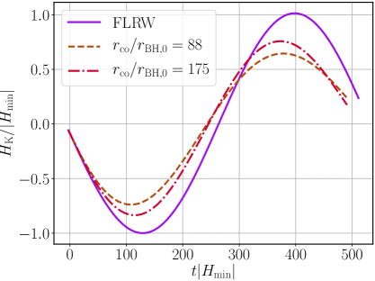
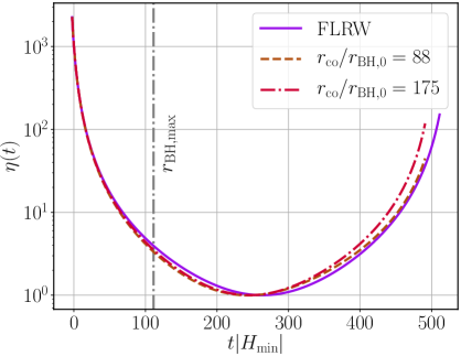
Figure 1: The expansion rate $H_{K}/|H_{\rm min}|$ computed from (3.4) (left) and the ratio of the matter to ghost field $\eta(t)$ given by (2.11) (right) for a black hole with initial mass such that the Hubble radius of the background cosmology $R_{\rm{H}}\equiv|H^{-1}|$ shrinks from an initial value of $R_{\rm{H},0}=75r_{\rm BH,0}$ to $4.34r_{\rm BH,0}$ (here $r_{\rm BH,0}$ is the initial black hole radius). The solid line shows the corresponding background solution, and the dashed and dash-dotted lines show the values at different coordinate radii. The vertical grey line is the time at which the black hole reaches its maximum areal radius as measured by the apparent horizon. Notice that the black hole reaches its maximum size slightly before the universe at large scales bounces, as the ghost field begins to dominate at an earlier time the closer one gets to the black hole horizon. The slight difference in the maximum absolute value of the FLRW value of $H_{\rm{K}}/|H_{\rm{min}}|$ at $t|H_{\rm{min}}|\sim 120,400$ is due to numerical error in our integration.

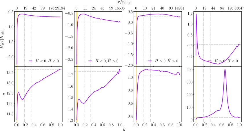
Figure 2: The expansion rate $H_{K}/|H_{\rm min}|$ (top) and the ratio of the energy densities of the matter to ghost field $\eta(t)$ given by (2.11) (bottom) for the black hole considered in figure 1 as a function of the compactified coordinate radius, $\hat{y}$ (see equation (A.1)), at different times during the evolution. Note that $\hat{y}$ lies along the “equator” of the black holes in our simulations. Also shown on the top axis is the proper radius of the spacetime computed from (3.7). The dashed horizontal grey lines indicate the corresponding background values at spatial infinity, the vertical dash-dotted lines correspond to the coordinate radii shown in figure 1, and the shaded region represents the black hole.

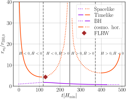
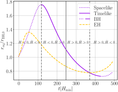
Figure 3: Left: The areal radii of the black hole (purple) and cosmological (orange) apparent horizons computed as described in section 3 for the black hole in figure 1. The line style reflects the signature of the marginally trapped tube or holographic screen (solid is timelike, dashed is spacelike). The diamond indicates the time and value to which the Hubble radius would shrink in the absence of a black hole. Right: The apparent horizon of the black hole (purple) and the corresponding event horizon (yellow dashed). The vertical solid line indicates the bounce, while the region between the dashed lines is the bouncing phase (where the NCC is violated).

We next present several results regarding the behavior of the area of the black hole, as measured by either the event or apparent horizon. Naively, one expects the accretion of the canonical/ghost field to result in an increase/decrease in mass of the black hole [82]. That being said, it is less clear how a black hole embedded in a cosmology driven by a canonical/ghost field may behave [83, 84].

Figure 3 depicts the evolution of the black hole’s areal radius. We find that during the contracting phase prior to the bouncing/NCC violation phase, the canonical scalar field energy density exceeds that of the ghost field; see figure 1 and the solid purple curve in figure 2. The black hole’s proper area increases during this time; (first region in figure 3 where $H<0,\dot{H}<0$). Once the bouncing phase starts ($t|H_{\rm min}|\sim 120$ in figure 1), the black hole starts to shrink as one may expect since the ghost field energy in this regime is comparable to the canonical scalar field energy density (second region where $H<0$ and $\dot{H}>0$ in figures 1 and 2). Near the end of the bouncing phase the universe is expanding (region where $H>0$ and $\dot{H}<0$), yet the black hole’s size is still shrinking in this region, as the ghost field energy density still dominates over the canonical scalar field energy density in the region near the black hole (in other words, $\eta<1$ in the region close to the black hole, see figure 2), although at an increasingly slower rate as the ghost field energy density quickly diminishes in time. After the end of the bouncing phase, the universe continues to expand, the ghost field decays to dynamically irrelevant values, and the black hole begins growing in size (fourth region where $H>0$ and $\dot{H}<0$ and the dotted purple curve).

The left panel of figure 3 also shows the areal radius of the cosmological horizon. We see that during the contracting phase, the cosmological horizon shrinks from $r_{\rm{C},0}=75r_{\rm{BH},0}$ to a minimum radius of $r_{\rm{C},\rm{min}}=4.34r_{\rm{BH},0}$ at $t\sim 50r_{\rm{BH},0}$. This is similar to the value the Hubble radius ($R_{\rm{H}}\equiv|1/H|$), would shrink to in the absence of a black hole. This value is indicated by the diamond in figure 3. From this we conclude that—at least in this regime—the presence of the black hole does not qualitatively change the dynamics of the spacetime. Past this point of closest encounter, the cosmological horizon tends to $r_{C}\to+\infty$ which defines the location of the bounce ($\lim_{H\to 0}1/H=\infty$). Once the universe switches from contraction to expansion, the cosmological horizon is defined as the location where the ingoing null expansion vanishes and outgoing null expansion is positive. After the bounce, the cosmological horizon at first shrinks to a minimum size before re-expanding to $+\infty$. We note that the areal radius of the cosmological horizon is no longer symmetric about the bounce once a black hole is present.

We also compute the signature of the MTTs associated with the horizons (see appendix B for definitions), which we plot in figure 3.

First we study the properties of the black hole MTT in more detail. Using the terminology of appendix B, the black hole is a future marginally trapped tube foliated by future marginally outer trapped surfaces (alternatively called a future holographic screen). The area law of dynamical horizons states that if the MTT is spacelike (i.e. if it is a dynamical horizon), then the area of the black hole should increase in the outward radial direction, while if the MTT is timelike (i.e. we have a timelike membrane with $\Theta_{(n)}<0$), then the area should increase into the past. Looking at figure 3 we find that (as expected) these laws are obeyed at all times, even during the bouncing phase.

We next look at the cosmological horizon. We consider the contracting and expanding phases separately. During the contracting phase, the cosmological horizon is a MTT foliated by future marginally inner trapped surfaces (alternatively, it is a future holographic screen). From the area law of future holographic screens [76, 77], we expect the cosmological horizon to obey the same area law as the black hole during the contracting phase. Our findings agree with this expectation: we find that the cosmological horizon is timelike when it decreases in time and spacelike when it increases in the outward direction. During the expanding phase, however, the cosmological horizon ceases to be a MTT. Instead, we find that it satisfies the definition of a past holographic screen (as the ingoing null expansion now vanishes). From [76, 77], we still expect its area to increase in the future on timelike portions and in the outward direction on spacelike portions. Again we find that this is satisfied at all times during the expanding phase.

We conclude by looking at the event horizon shown in the right panel of figure 3. Our main finding here is that the event horizon no longer lies outside the apparent horizon at all times. This is a result of the violation of the NCC [42]. Interestingly, this behavior begins not during the bouncing phase of cosmological evolution (between the two dashed grey lines) when the NCC is violated, but before the bouncing phase has begun. This is because the event horizon is not a quasi-local quantity, so it can “anticipate” the bouncing/NCC violation phase. In general, we find that the event horizon always increase until it crosses the apparent horizon of the black hole, after which it decreases. Once the bouncing phase ends, the event horizon crosses the apparent horizon again, after which it starts increasing and remains larger than it for all future times.

We were not able to evolve the spacetime to arbitrarily large proper times. We ascribe this to gauge artefacts which impede the stable numerical evolution of the solution. In particular, the lapse function appears to become distorted in the spacetime region between the black hole and the asymptotically homogeneous regime, which causes that interior region to advance in time much faster compared to elsewhere in the simulation. (This is evident in the rightmost panels of figures 1, 4, and 12.) That being said, based on the simulations we have run, we conjecture that the black hole asymptotes to close to its initial mass at $t\to\infty$ with no significant gain or loss of energy. That is, the end state is described by a black hole embedded in an expanding matter like FLRW universe with a negligible amount of ghost field and matter energy density. This is illustrated in figure 13 of appendix A where we consider a black hole with half the mass of the one depicted in figure 3, i.e. we consider a black hole such that the ratio of the minimum Hubble radius to the initial radius of the black hole is $R_{\rm{H},\rm{min}}/r_{\rm{BH},0}=8.69$. Figure 13 shows that, overall, the black hole’s size changes by a negligible amount. In this particular case, the final size of the apparent horizon of the black hole is $\sim 6\%$ larger that its initial value, the small difference being an artefact of the initial data. More importantly, figure 13 also shows that the event horizon asymptotes to the apparent horizon at late times.

4.2 Large black hole regime

We next consider solutions where $R_{\rm{H},\rm{min}}/r_{\rm{BH},0}<3.5$. The nonlinear evolution of one particular case is shown in figure 4. As is the case for the lower initial mass evolutions (figure 1), we see that the cosmological evolution remains unaffected far away from the black hole. The bounce is pushed to even earlier times, as one may expect since a large black hole could presumably accelerate the rate of cosmological contraction. Figure 5 shows that in the region near the black hole apparent horizon, the local expansion rate and the ratio of the energy densities now differ from their background value by up to $15$–$75\%$ and $13$–$60\%$. Beyond $r\sim 2$–$12r_{\rm{BH},0}$, both quantities asymptote to their respective background values.

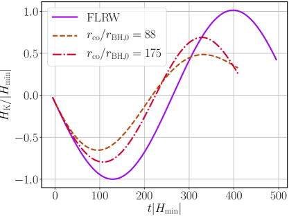
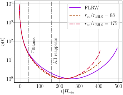
Figure 4: Same as figure 1, but for a black hole with initial mass such that the Hubble radius of the background cosmology $R_{\rm{H}}\equiv|H^{-1}|$ shrinks from an initial value of $R_{\rm{H},0}=75r_{\rm BH,0}$ to $2.17r_{\rm BH,0}$ (here $r_{\rm BH,0}$ is the initial black hole radius).

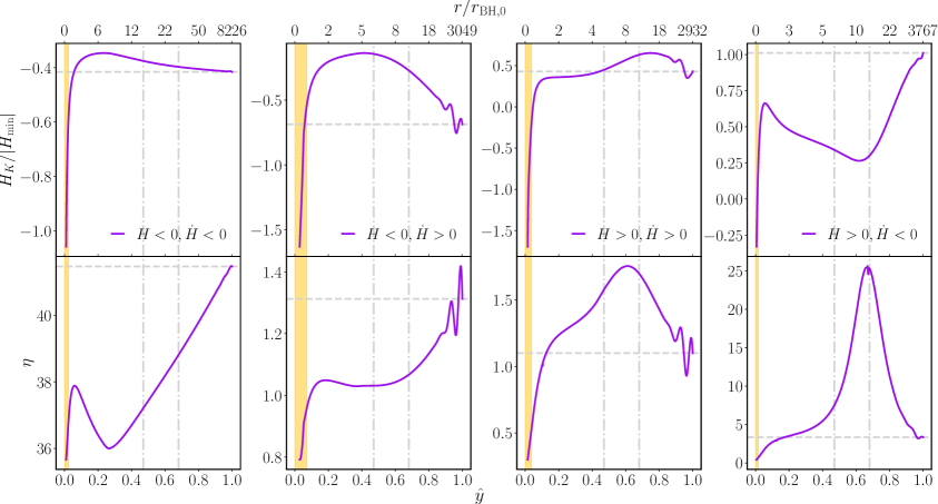
Figure 5: Same as figure 2, but for the case with $R_{\rm H,min}/r_{\rm BH,0}=2.17$ also shown in figure 4.

The behavior of the black hole and cosmological apparent horizons, which is shown in figure 6, is qualitatively different for the large black hole initial data as compared to the small black hole initial data ($R_{\rm{H},\rm{min}}/r_{\rm{BH},0}\gtrsim 3.5$). Similar to the cases studied in the section 4.1, the cosmological horizon shrinks at first. Unlike those earlier cases though, it eventually merges with the expanding black hole apparent horizon. Following the merger, the spacetime has no apparent horizons for some time until they re-emerge. After that, the cosmological and black hole apparent horizons follow a similar trajectory to the horizons studied in section 4.1 during the cosmological expansion phase.

The merging of black hole and cosmological apparent horizons has been observed in McVittie spacetimes [85, 86] (see also appendix C) and can be interpreted the following way. As the apparent horizon of the black hole grows and the cosmological horizon shrinks during the contraction of the universe, we reach a point in time at which the black hole horizon coincides with the cosmological horizon. At this point, one cannot distinguish between the black hole and the cosmological horizon (recall that during the contraction the outward null expansion is negative outside of the cosmological horizon). A finite time later, before the bounce, but after the background Hubble radius reaches its minimum size, the effective Hubble radius has increased to a sufficiently large value so that the black hole solution again fits within the cosmological horizon. At this point, the cosmological and black hole apparent horizons reappear. We note that the black hole event horizon persists throughout the evolution of the spacetime, so in this sense the black hole never disappears; see figure 6. We next investigate the physical properties of this process in more detail.

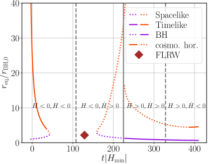
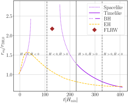
Figure 6: Same as figure 3 but for a black with initial mass such that the Hubble radius of the background cosmology $R_{\rm{H}}\equiv|H^{-1}|$ shrinks from an initial value of $R_{\rm{H},0}=75r_{\rm BH,0}$ to $2.17r_{\rm BH,0}$ (here $r_{\rm BH,0}$ is the initial black hole radius). Notice that the location where $H=0$ (that is, where the Hubble radius diverges) does not exactly coincide to where the cosmological horizon blows up, as the cosmological horizon is measured locally (in the interior of the computational domain), while $H=0$ is determined by the asymptotic cosmological evolution. For more discussion on how we define the cosmological horizon, see section 3

We first address the question of whether a naked singularity forms after the black hole and cosmological horizons collide [83, 86, 85]. The formation of a naked singularity would signal a breakdown of the theory—either through the formation of a blowup in curvature, or through necessitating new boundary conditions to be set at the singularity boundary [87]. Our simulations suggest no naked singularity is formed. More concretely, the outward null expansion during this period is negative everywhere, so the entire spacetime is essentially trapped, and no new boundary conditions need to be specified. In particular, we can continue to excise a central region corresponding to the inside of the black hole. Additionally, considering the event horizon shown in figure 6, we see that it remains finite at all times. Note that just like in the case studied earlier in section 4.1, the event horizon is smaller than the apparent horizon before, and during the bouncing phase, and turns around when it crosses the apparent horizon.

We next consider the behavior of the marginally (anti-)trapped tubes and their signature, shown in figure 6. Note that while the black hole MTT is spacelike and increasing in time before it merges with the cosmological horizon, when it reappears from the merger, its signature remains spacelike even though its area continues to decrease in time. Since the area of the black hole always increases in the outward radial direction, this implies that while the outward direction points into the future before the merger, it points into the past when it reappears. The black hole apparent horizon undergoes another signature change at the bounce (indicated by the grey vertical solid line) after which it behaves like the case studied above (i.e. the signature of the horizon becomes timelike, and decreases as we evolve forwards in time). Similarly, we find that the cosmological horizon follows the same trend as the case in section 4.1, except for a brief period of time just before it merges with the black hole apparent horizon: here the horizon signature becomes spacelike. We see that the cosmological horizon and black hole apparent horizons have the same signature when they annihilate and re-emerge.

A natural question to ask is whether the collision of the apparent horizons during the contraction phase is an artefact of the particular matter model we use, or is a more general consequence of a contracting universe. To explore this, we consider the same initial conditions as the ones used in figure 4, but now evolve only with the canonically normalized scalar field. The results of this are plotted in figure 7. We find that during contraction, the apparent horizons, with and without the presence of a ghost scalar field, behave in a similar fashion. In both cases, the black hole apparent horizon merges with the cosmological horizon at the same areal radius. This is in line with our earlier observation that the black hole horizon’s size exceeds the cosmological horizon before the bouncing phase starts, (i.e. before the ghost field has a significant impact on the evolution of the system). The black hole and cosmological apparent horizon merge earlier by around $t\sim 2|H_{\rm min}|$ in the case of contraction without the ghost scalar field. This is consistent with the notion that the accretion of the ghost field should slow down the rate at which the black hole can grow in size, which would delay the time of merger of the two horizon.

Finally, we note that the signature of the cosmological horizon becomes spacelike in this setup just before merging with the black hole horizon for both cases. During this phase of evolution, the cosmological horizon is a dynamical horizon whose area decreases with time.

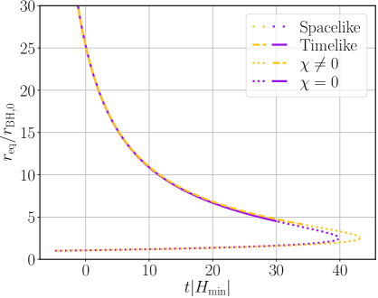
Figure 7: Cosmological and black hole apparent horizons from the contracting phase of the same case shown in figure 6 (labelled $\chi\neq 0$) compared to a similar case without a ghost field ($\chi=0$).

4.3 Dependence on black hole size

In this section, we explore in more detail how the properties of the spacetime during the bounce change as a function of $R_{\rm{H},\rm{min}}/r_{\rm{BH},0}$.

As described in section 4.1, for initial data where $R_{\rm{H},\rm{min}}\approx 4.34r_{\rm BH,0}$ the black hole apparent horizon persists through the whole bounce, and the spacetime evolution near the black hole qualitatively resembles the asymptotic cosmological evolution. As this behavior will hold to an even greater degree for smaller black holes (relative to $R_{\rm{H},\rm{min}}$), we are more interested in the opposite regime, considering larger black holes. As mentioned in section 1, for astrophysical black holes we expect $R_{\rm{H},\rm{min}}\ll r_{\rm BH}$. We find that, when $R_{\rm{H},\rm{min}}\lesssim 3.5r_{\rm BH,0}$, (see section 4.2), the black hole apparent horizon collides with the cosmological horizon while the universe is still contracting. In this section, we therefore explore how this behaviour changes as one increases the initial mass of the black hole. We note that for numerical reasons, we will restrict to evolutions where $R_{\rm{H},\rm{min}}>0.86r_{\rm BH,0}$. However, as we argue below, we already see some consistent trends as $r_{\rm BH}$ is varied within this regime.

In the left panel of figure 8, we plot the radius of the black hole apparent horizon normalized by its initial value as a function of time. For evolutions where the black hole and cosmological MTTs do not collide, we find that although the area of the apparent horizon always reaches it maximum and minimum values at around the same harmonic time ($t\sim 110R_{\rm H,min}$ for the maximum value, and $t\sim 440R_{\rm H,min}$ for the minimum value), the value the maximum and minimum take does change as a function of initial black hole area. Independently of the black hole’s initial size, the area of the apparent horizon is close to one around the bounce or in other words around the time where the total energy density of the background cosmology is zero. In the low mass regime, the variation in the black hole’s size increases with increasing initial black hole area.

However as the initial size of the black hole increases, the maximum change in the radius of the apparent horizon eventually peaks at a value of $r_{\rm AH,max}/r_{\rm AH,0}\sim 2.6$. In this case, the ratio of the minimum Hubble radius of background cosmology to initial radius of the black hole corresponds to the threshold beyond which the horizons merge. Beyond this peak, although the horizons merge at successively earlier times (and always before the bouncing phase starts), with increasing initial black hole radius, the relative increase in the radius of the apparent horizon when the horizons merge saturates at a value of $r_{\rm AH,max}/r_{\rm AH,0}\sim 2.5$. Within the range of masses we were able to evolve, the apparent horizons always reappear, from which we conjecture that the presence of black holes in bouncing cosmologies do not disrupt the bounce. We were not able to evolve the space time to arbitrarily later proper time but based on all the simulations we have run, we conjecture that the black hole asymptotes to close to its initial radius as $t\rightarrow\infty$ .

In the right panel of figure 8, we plot the radius of the black hole event horizon normalized by its initial value as a function of time. We do not compute the evolution of the event horizon past the bounce for black holes with initial black hole radius such that the minimum Hubble radius is smaller than $R_{\rm{H},\rm{min}}<2.90r_{\rm BH,0}$, as for those cases the event horizon cannot be located to the desired accuracy (see appendix A for more details on the computation of the event horizon). For the set of initial radii we do compute, we find that the area of the event horizon reaches a maximum at successively earlier times with increasing initial black hole radius, always before the bouncing phase starts and always when the event horizon crosses the apparent horizon of the black hole. Beyond this point, the event horizon decreases in size, until it crosses the apparent horizon again, after which it starts increasing. This minimum happens at successively earlier times with increasing initial black hole radius. While the maximum size of the event horizon throughout the evolution increases with increasing initial black hole radius, the minimum decreases.

We next argue that the behavior of the event horizon in the region leading up to the bounce (where $H<0$), can be at least qualitatively captured by studying null rays in the background FLRW spacetime. The reasoning is as follows: It is reasonable to assume that in the regime where $R_{\rm H}/r_{\rm BH,0}\gg 1$, the evolution of null rays near the black hole horizon will not be greatly influenced by the background cosmological evolution. Likewise, we assume that in the regime where the black hole is “large” ($R_{\rm H}/r_{\rm BH,0}\lesssim 1$), the trajectories of null rays exterior to the black hole are more influenced by the cosmological evolution, and in the background FLRW spacetime, during the contraction phase, outward radial null rays have decreasing proper radius when they are inside the Hubble radius. Following this line of thought, we integrate null rays backward in time in the background FLRW spacetime given by eq. 2.3, starting from the latest time for which $H<0$ and $R_{\rm H}=r_{\rm BH,0}$. Figure 9 shows the trajectories of a few such null rays for different ratios of $R_{\rm H,min}/r_{\rm BH,0}$. We find that the proper radius of the null rays increases (as we go backwards in time) until the ray crosses $R_{\rm H}$, after which it decreases. This is consistent with the behavior of the event horizon in the right panel of figure 8 and suggests that, at least for this part of the evolution, the size of the black hole is determined by the evolution of the background cosmology. This simple calculation also shows that as $R_{\rm H,min}/r_{\rm BH,0}$ decreases, the maximum radius of the null ray increases. This agrees with what we see in our full numerical simulations. Extrapolating this trend to arbitrarily small $R_{\rm H,min}/r_{\rm BH,0}$ suggests that for arbitrarily large black holes the peak of the event horizon will diverge. However, we are working with a cosmological solution that has undergone an infinite number of e-folds of contraction to the past (see section 2.2). If one were to consider a bouncing model that had only had a finite period of contraction (for example if we considered a cyclic cosmology [47]), then the maximum of the event horizon would always be finite.

Evolving forward in time, into the region where the universe is expanding ($H>0$), we find that the event horizon continues to decrease until it crosses the apparent horizon, at which point it begins to increase in size. However, this behavior can not be captured by integrating the null geodesics in the background spacetime, which suggests that the influence of the black hole on the geometry is more relevant when $H>0$, and for radii less than $r_{\rm BH,0}$. Due to numerical issues, we are unable to evolve far enough in time to determine if the minimum of the event horizon keeps decreasing and eventually reaches a point where the event horizon ceases to exist as $R_{\rm H,min}/r_{\rm BH,0}\rightarrow 0$.

Finally, we note that (as is shown in figure 13) one expects the apparent and event horizons to converge to the same value at late times, but for reasons mentioned earlier in this section, we are not able to evolve long enough in time to show this happens for initial data with $R_{\rm{H},\rm{min}}<4.34r_{\rm BH,0}$.

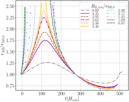
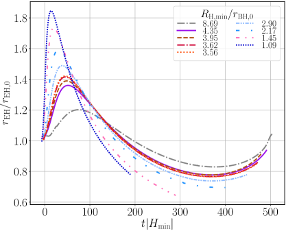
Figure 8: Radius of the apparent (left) and event (right) horizon of the black hole over time for different ratios of the minimum Hubble radius to initial black hole radius.

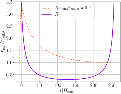
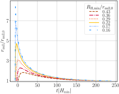
Figure 9: Proper radius of outward, radial null rays in the background FLRW spacetime (described in section 2.1). The left panel shows an example null ray that begins at a specified radius $r_{\rm null,0}$, increases until it crosses the Hubble radius (during contraction), and then decreases until it reaches the Hubble radius again at $r_{\rm null,0}$. The right panel shows the same thing for different ratios of the minimum Hubble radius to $r_{\rm null,0}$.

4.4 Spinning black holes

Up to this point, we have only considered non-spinning black holes (spherically symmetric spacetimes). However, our methods can be applied equally well to spinning black holes spacetimes. We have considered several such cases, finding the same qualitative behavior as for non-spinning black hole initial data. We illustrate this with a representative example case: initial data where the black hole is initially spinning with a dimensionless spin value of $a_{0}=0.5$. As we find little difference compared to the spacetimes with non-spinning black holes, here we only present the results for a black hole with $R_{\rm H,min}=2.17r_{\rm BH,0}$, and the same mass as in section 4.2. Figure 10 compares the circumferential radius of the black hole along the equator for the spinning and non-spinning cases. We find that the addition of spin causes the horizons to merge at a slightly later time as compared to a comparable non-spinning case. We do not plot the behavior of the asymptotic background cosmology as it is the same regardless of whether the black hole is spinning or not. As was mentioned in section  3, the angular momentum of the black hole is constant since the scalar field does not carry angular momentum.

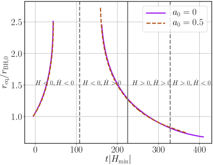
Figure 10: The circumferential radius of the black hole in figure 6 with zero spin ($a=0$) compared to dimensionless spin of $a=0.5$.

5 Discussion and conclusion

We have considered the first numerical evolution of black holes through a nonsingular bouncing cosmology. As in [30, 32], we worked with a model that has two scalar fields: a canonically normalized field with an exponential potential and a ghost field. We have additionally considered asymptotically cosmological initial data that is tuned to allow for a matter-like (effective equation of state $w=0$) contraction which is then followed by a bounce that ends with cosmological expansion. In [32], translational symmetries were assumed in two spatial directions, which precludes the formation of black holes. By contrast, in this work we considered axisymmetric spacetimes which allowed us to study the behavior of black holes through a bounce. While only a small fraction of Hubble patches are expected to have a black hole during the late stages of ekpyrotic contraction [4, 36, 46], our setup allows us to examine the robustness of the ghost-field bounce, which in turn serves as an effective classical model of NCC violation.

We found two qualitatively different kinds of spacetime evolution, which depended on the ratio of the minimum Hubble radius of the background cosmology to the initial radius of the black hole. For black holes with initial radius smaller than $\sim 3.5$ times the minimum size of the Hubble radius of the background cosmology, the black hole passes through the bounce freely and the background cosmology remains largely unaffected (see section (4.1)). Beyond this limit, we found that while regions far away from the black hole still bounce freely, regions close to the black hole evolve differently (see section (4.2)). In particular, we found that during the contracting phase, the cosmological horizon and the black hole apparent horizon merge and cease to exist for a brief period of time. Some finite time later, before the bounce but after the background Hubble radius reached its minimum size, the cosmological and black hole apparent horizons separate. Within the range of masses we considered, we found that the black hole size (as measured by its horizon radius), varies significantly during its evolution. However, regardless of the initial mass of the black hole, we found that the late time evolution consists of a black hole in an expanding universe with a mass similar to its initial value. Although we were not able to evolve spacetimes where the Hubble radius shrinks to a much smaller size compared to the radius of the black hole, we conjecture that the black hole always survives through the bounce. This means that black holes created (or already present) in the contraction phase [36, 46] can persist to have observational consequences in the post-bounce era.

We found instances where the event and apparent horizons decrease as a result of our spacetime violating the NCC. Independently of the NCC being violated, we found that in the regime where the black hole and cosmological apparent horizon collide, the latter becomes spacelike shortly before merging with the black hole. This is consistent with the observation that the signature of the marginally (anti-)trapped tubes changes such that any merging/reappearing pair of horizons always has the same signature.

Finally, we point out a few directions for future research. One would be to study the dynamics in a setup where the asymptotic cosmology is not prescribed. For example, this could be accomplished by considering a toroidal/periodic setup, and then considering a “lattice” of black holes [55, 34]. This setting would allow for the study of the impact of black holes, as well as other perturbations on the overall dynamics of the bounce. While small perturbations have not been found to appreciably change the dynamics of a nonlinear bounce when translational symmetries are assumed [32], it would be interesting to see if perturbations could be more disruptive in the presence of a black hole, and in a less-symmetric spacetime that does not preclude large-scale anisotropies.

Another direction would be to consider other models of cosmological bounces. While we believe that the main conclusions we find here do not depend strongly on the details of the bounce model, it would be interesting to determine what differences would result from potentially more realistic models of a bounce. As we mention in the Introduction, the cosmological bounce scale may be many orders of magnitude smaller than the initial size of a primordial black hole. Due to the numerical instabilities (as described in Sec. 4.2), we were unable to carry out evolutions in the regime $R_{\rm H,min}/R_{\rm BH,0}\ll 1$. It would be interesting to see if our results still hold in this limit.

Another interesting question is the degree to which a ghost field, which can reverse cosmic contraction, may similarly affect gravitational collapse and singularity formation in a black hole interior. NCC violating fields such as ghost fields have been used to construct singularity free black hole-like solutions, such as wormholes [88, 89, 90, 91], so it is not entirely implausible that there could be nontrivial dynamics near the center of a black hole that accretes a ghost field. In this study, we ignored the dynamics deep inside the black hole, excising that region from our domain. Exploring this would require coordinates better adapted to studying the interior of black hole spacetimes, such as null coordinates [92].

Appendix A Numerical methodology

We solve the equations of motion (2.2) using the generalized harmonic formulation as described in [93]. The numerical scheme we use follows that of [94], which we briefly summarize here. We discretize the partial differential equations in space, using standard fourth-order finite difference stencils, and in time, using fourth-order Runge-Kutta integration. We control high frequency numerical noise using Kreiss-Oliger dissipation [95]. We use constraint damping to control the constraint violating modes sourced by truncation error, with damping parameter values similar to those used in black hole evolutions using the generalized harmonic formulation [93]. We fix the gauge freedom by working in harmonic coordinates, $\Box x^{\alpha}=0$. During the expansion phase, we dynamically adjust the time step size in proportion to the decreasing global minimum of $1/\alpha$ where $\alpha$ is the lapse (this would be $\alpha=1/a^{3}$ in a homogeneous FLRW universe, see eq. (2.3)) in order to avoid violating the Courant-Friedrichs-Lewy condition [57, 96].

Following [97], we dynamically track the outer apparent horizon of the black hole, and excise an ellipsoid-shaped region interior the horizon. We typically set the ratio of the maximum ellipsoid axis to the maximum black hole radial value to be $0.6$.

We compute the event horizon by integrating null surfaces backwards in time [70, 71, 72] (we restrict this to spherically symmetric cases, where it is sufficient to consider spherical null surfaces). Since we are not able to evolve the spacetime to infinite proper time (at which point the event and apparent horizon would coincide), we cannot precisely determine the final position of the event horizon. Instead, we use the apparent horizon as the approximate location of the event horizon and choose a range of initial guesses around this value. For two surfaces initially separated by $2.5r_{\rm{BH},0}$, we find that their separation decreases to $0.1r_{\rm{BH},0}$ within $\sim 4\times 10^{-3}|H_{\rm min}|^{-1}$ when evolving the null surfaces backwards in time, after which we consider the location of the event horizon to be accurate to the desired accuracy. Note that the separation rapidly decreases when integrating backwards in time, a direct consequence of the divergence of the null geodesics going forward in time [71].

We additionally make the use of compactified coordinates so that physical boundary conditions can be placed at spatial infinity [97]:

$$x^{i}=\tan\left(\frac{\pi\hat{x}^{i}}{2}\right),$$ (A.1)

so that $\hat{x}^{i}=1$ corresponds to $x^{i}=\infty$. Unlike in [97] though, we work in an asymptotically FLRW spacetime instead of an asymptotically flat spacetime, similar to what is done in [44]. That is, at our spatial boundary we set

$$g_{tt}=-\alpha(t)^{2},\qquad g_{ti}=0,\qquad g_{ij}=a(t)^{2}\delta_{ij},$$ (A.2)

where the lapse $\alpha(t)=a(t)^{3}$; and the scale factor $a(t)$ satisfies the Friedmann equations, eq. (2.4).

We use Berger-Oliger [98] style adaptive mesh refinement (AMR) supported by the PAMR/AMRD library [99, 100]. Typically our simulations have 9–12 AMR levels (using a $2:1$ refinement ratio), with each nested box centered on the initial black hole and between 128 and 256 points across the x-direction on the coarsest AMR level. The interpolation in time for the AMR boundaries is only third-order accurate, which can reduce the overall convergence to this order in some instances. As we restrict to axisymmetric spacetimes, we use the modified Cartoon method to reduce our computational domain to a two-dimensional Cartesian half-plane [97].

We construct initial data describing a black hole of mass $M(t=0)=M_{0}$ in an initially contracting FLRW spacetime described in section 2.2. We solve the constraint equations using the conformal thin sandwich formalism, as described in [65]. More precisely, we choose the initial time slice to have constant extrinsic curvature $K=-3H_{0}$ where $H_{0}=\mathcal{H}_{0}{a_{0}}^{-3}$ is given by (2.4d), and the initial values for $\{\phi,\phi^{\prime},\chi,\chi^{\prime},a,a^{\prime}\}$ are fixed by (2.10) (a similar approach was employed in [57, 44]). Without loss of generality, we choose the initial value of the ratio between the energy density of the $\phi$ and $\chi$ fields and $V_{0}$ to be such that during the contraction phase, the Hubble radius of the background cosmology $R_{H}\equiv|H^{-1}|$ shrinks from an initial value of $R_{H}(t=0)=75r_{\rm BH,0}$ to $4.34r_{\rm BH,0}$ (here $r_{\rm BH,0}$ is the initial black hole radius). We considered a range of initial black hole masses, keeping the initial ratio of Hubble to black hole radius to be 75, but changing the minimum Hubble to initial black hole radius ratio from $4.34r_{\rm BH,0}$ all the way to $0.87r_{\rm BH,0}$. We also study some black holes with an initial dimensionless spin of $a_{0}=0.5$.

Finally, we present a convergence test of our code and setup. In figure 11, we present the time evolution of the apparent horizon of the black hole and the norm of the constraint violations $C^{\alpha}\equiv\Box x^{\alpha}$ integrated over the coordinate radius $r\leq 265M_{0}$, for a non-spinning black hole with initial mass such that $R_{\rm{H},\rm{min}}=1.45r_{\rm BH,0}$, for different numerical resolutions. For this case, the lowest resolution is 128 points across the x-direction on the coarsest AMR level with 10 levels of mesh refinement and a spatial resolution of $dx/M_{0}\approx 0.004$ on the finest level. The medium and high resolutions correspond, respectively, to an increased resolution of $3/2$ and $2\times$ that of the lowest resolution run. We find that the constraints converge to zero at roughly third order. This is because the convergence is dominated by the third order time interpolation on the AMR boundaries. The medium resolution in the convergence study is equivalent to the resolution we use for all the other cases studied here. We place the mesh refinement such that the radius of the black hole resides inside the finest AMR level initially. During the evolution, the mesh refinement is adjusted according to truncation error estimates to maintain roughly the same level of error.

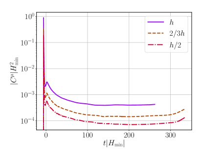
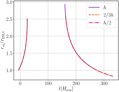
Figure 11: The integrated norm (left) of the constraint violations $C^{\alpha}\equiv\Box x^{\alpha}$ integrated over the coordinate radius $r\leq 265M_{0}$ and the apparent horizon (right), for a black hole with initial radius such that $R_{\rm{H},\rm{min}}=1.45r_{\rm BH,0}$, for different resolutions. The medium (high) resolution case has $1.5\times$ ($2\times$) the resolution of the low resolution, and the convergence is consistent with third order.

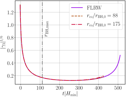
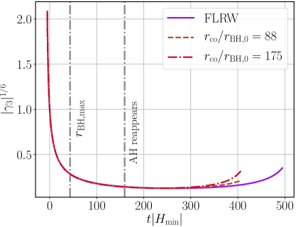
Figure 12: The effective scale factor $|\gamma_{3}|^{1/6}$ computed from (3.6) for a black hole with initial mass such that the Hubble radius of the background cosmology $R_{\rm{H}}\equiv|H^{-1}|$ shrinks from an initial value of $R_{\rm{H},0}=75r_{\rm BH,0}$ to $4.34r_{\rm BH,0}$ (left)/$2.17r_{\rm BH,0}$ (right). The solid line shows the corresponding background solution and the dashed and dash-dotted lines the values at different coordinate radii. The vertical grey line is the time at which the black hole reaches its maximum mass as observed by the apparent horizon.

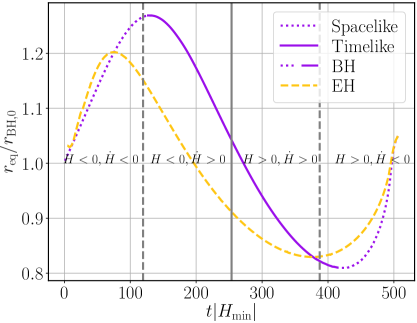
Figure 13: The apparent horizon of the black hole (purple) and the corresponding event horizon (yellow dashed) for a black hole with initial mass such that the Hubble radius of the background cosmology $R_{\rm{H}}\equiv|H^{-1}|$ shrinks from an initial value of $R_{\rm{H},0}=75r_{\rm BH,0}$ to $8.69r_{\rm BH,0}$. The vertical solid line indicates the bounce, while the region between the dashed lines is the bouncing phase (where the NCC is violated). The line style of the apparent horizon reflects the signature of the marginally trapped tube or holographic screen (solid is timelike, dashed is spacelike).

Appendix B Various notions of black hole and cosmological horizons

B.1 General definitions and properties

Nonsingular classically bouncing cosmologies require the violation of the NCC [10, 11, 30, 4, 5]. The NCC plays a fundamental fundamental role in the classical area law for black holes [42, 101]. Given this, we pay particular attention to the dynamics of the black hole horizon in our simulations. In addition to the event horizon (which can only be computed once the whole spacetime is known [72]), there are several other quasi-local definitions of black hole horizons which we measure: dynamical horizons [102, 81, 80], apparent horizons [102, 103, 79, 81, 80, 104, 33], and holographic screens [75, 76, 77] (also called marginally trapped tubes [78]).

For completeness, we collect the definitions and some of the basic properties of these horizons in this appendix. Wherever applicable, we also discuss how these definitions can be extended to define cosmological horizons. We refer the reader to [102, 103, 79, 81, 80, 104, 33, 75, 76, 77] for more thorough reviews on this subject.

• Trapped surfaces and apparent horizons
  Let $\mathcal{S}$ be a smooth, closed, orientable spacelike two-dimensional submanifold in a four-dimensional spacetime $(\mathcal{M},g_{ab})$. We then define two linearly independent, future-directed, null vectors normal to $\mathcal{S}$, normalized such that

  $$g_{\alpha\beta}l^{\alpha}n^{\beta}=-1$$ (B.1)

  where by convention $l^{\alpha}$ and $n^{\beta}$ are respectively the outgoing and ingoing null normals. The two-metric induced on $\mathcal{S}$ is

  $$\tilde{q}_{\alpha\beta}=g_{\alpha\beta}+l_{\alpha}n_{\beta}+n_{\alpha}l_{\beta},$$ (B.2)

  and the null expansions are defined as

  $$\Theta_{(l)}\equiv\tilde{q}^{\alpha\beta}\nabla_{\alpha}l_{\beta},\qquad\Theta_{(n)}\equiv\tilde{q}^{\alpha\beta}\nabla_{\alpha}n_{\beta}.$$ (B.3)

  The closed two-surface $\mathcal{S}$ is a trapped surface if the outgoing and ingoing expansions are strictly negative i.e. if $\{\Theta_{(l)}<0,\Theta_{(n)}<0\}$ and a marginal trapped surface if the outgoing null expansion vanishes i.e if $\{\Theta_{(l)}=0,\Theta_{(n)}<0\}$. Conversely, the closed two-surface $\mathcal{S}$ is am anti-trapped surface if the outgoing and ingoing expansions are strictly positive i.e. if $\{\Theta_{(l)}>0,\Theta_{(n)}>0\}$ and a marginal anti-trapped surface if the ingoing null expansion vanishes i.e if $\{\Theta_{(l)}>0,\Theta_{(n)}=0\}$.

  A marginal trapped surface ($\Theta_{(l)}=0$) is future if $\Theta_{(n)}<0$, past if $\Theta_{(n)}>0$, outer if $\mathcal{L}_{(n)}\Theta_{(l)}<0$ and inner if $\mathcal{L}_{(n)}\Theta_{(l)}>0$. Conversely, a marginal anti-trapped surface ($\Theta_{(n)}=0$) is future if $\Theta_{(l)}<0$, past if $\Theta_{(l)}>0$, outer if $\mathcal{L}_{(l)}\Theta_{(n)}<0$ and inner if $\mathcal{L}_{(l)}\Theta_{(n)}>0$.
  

  A black hole apparent horizon is a future marginally outer trapped surface. Within the context of cosmology, the cosmological apparent horizon of an expanding FLRW spacetime is a past marginally inner anti-trapped surface. For a contracting FLRW spacetime, the cosmological apparent horizon is a future marginally inner trapped surface.

• Dynamical horizons and holographic screens
  We now have all the ingredients to introduce the concept of a Marginally Trapped Tube (MTT): A MTT is a smooth, three-dimensional submanifold that is foliated by MTSs. If a MTT is everywhere spacelike, it is referred to as a dynamical horizon [80, 81]. If it is everywhere timelike, it is called a timelike membrane (TLM). Finally, if it is everywhere null then we have an isolated horizon.

  We next outline the various ingredients that go into the area law of dynamical horizons (the quasi-local horizon that appears the most frequently in our numerical solutions). It is straightforward to derive an area law for purely spacelike or purely timelike dynamical horizons. Consider first the spacelike case. Let $H$ be a dynamical horizon and $\mathcal{S}$ be a member of the foliation of future marginally trapped surfaces. Since $H$ is spacelike, we can define a future-directed unit timelike vector normal to $H$, $\hat{\tau}^{a}$ and a unit outward pointing spacelike vector tangent to $H$ and normal to the cross-sections of $H$, $\hat{r}^{\alpha}$. A suitable set of null normals is then

  $$l^{\alpha}=\frac{1}{\sqrt{2}}(\hat{\tau}^{\alpha}+\hat{r}^{\alpha}),\ \ \ n^{\alpha}=\frac{1}{\sqrt{2}}(\hat{\tau}^{\alpha}-\hat{r}^{\alpha}).$$ (B.4)

  Then since (by the definition of a dynamical horizon) $\Theta_{(l)}=0$ and $\Theta_{(n)}<0$, it follows that the extrinsic curvature scalar of $\mathcal{S}$ is

  $$\tilde{K}={\tilde{q}}^{\alpha\beta}D_{\alpha}\hat{r}_{\beta}=-\frac{\Theta_{(n)}}{\sqrt{2}}>0,$$ (B.5)

  where $D_{\alpha}$ is the covariant derivative operator on $H$. This shows that the area of the cross-sections of a spacelike dynamical horizon increases along $\hat{r}^{\alpha}$. We emphasize that this does not necessarily imply that the area increases in time. In spherical symmetry, we explicitly show below (section B.2) that the outward vector points in the future when the area increases in time and in the past when the area decreases in time. For a timelike dynamical horizon, the roles of $\hat{\tau}^{\alpha}$ and $\hat{r}^{\alpha}$ are interchanged. In this case, $\hat{r}^{\alpha}$ is no longer tangential to $H$, and is instead the unit spacelike vector normal to $H$. Additionally, $\hat{\tau}^{\alpha}$ is instead the unit timelike vector tangent to $H$ and orthogonal to the cross-sections of $H$. The area law then becomes

  $$\tilde{K}=\tilde{q}^{\alpha\beta}D_{\alpha}{\hat{\tau}}_{\beta}=+\frac{\Theta_{(n)}}{\sqrt{2}}<0,$$ (B.6)

  i.e. the area of a timelike dynamical horizons decreases along ${\hat{\tau}}^{\alpha}$. Note this law does not rely on any energy conditions, such as the NCC.

  Finally, we note that the area law defined in [80, 81] only applies to dynamical horizons and timelike membranes. The definition does not include marginally anti-trapped tubes, which are often present in cosmological settings, or marginally trapped tubes which may not have a definite signature at a given time. To remedy this, Bousso and Engelhardt [76, 77] formulated and proved a new area theorem applicable to an entire hypersurface $H$ of indefinite signature. The area theorem is based on a few technical assumptions but should be applicable to most hypersurfaces foliated by marginally trapped or anti-trapped surfaces $\mathcal{S}$, called leaves. In this context, marginally (anti-)trapped tubes are referred to as future (or past) holographic screens. More precisely, the Bousso-Engelhardt area theorem is: the area of the leaves of any future (past) holographic screen, $H$, increases monotonically along $H$. The direction of increase along a future (past) holographic screen is the past (future) on timelike portions of $H$ or exterior on spacelike portions of $H$. Thus $H$ only evolves into the past (future) and/or exterior of each leaf.

B.2 Dynamical horizons and timelike membranes in spherical symmetry

As most of our simulations are performed in an essentially spherically symmetric spacetime, here we consider the properties of dynamical horizons for these spacetimes in more detail. The main purpose of this section is to illustrate how the area law for dynamical horizons [80, 81] reduces to an essentially tautological statement about the dynamics of the horizon area.

We use $r$ to denote the areal radius, and we will work with a gauge such that $r$ is also a coordinate of the spacetime, that is we will consider a metric of the form

$$ds^{2}=\alpha_{ab}dx^{a}dx^{b}+r^{2}\left(d\vartheta^{2}+\sin^{2}\theta d\varphi^{2}\right),$$ (B.7)

where $\alpha_{ab}$ is a two-dimensional metric that is function of $(t,r)$ (here $t$ is the timelike coordinate). We recall that in spherical symmetry the expansion for a null vector $v^{\mu}$ is [105]

$$\Theta_{(v)}=\frac{1}{4\pi r^{2}}v^{\alpha}\partial_{\alpha}\left(4\pi r^{2}\right)=\frac{2}{r}v^{r}.$$ (B.8)

The last expression follows from our imposing a gauge such that the areal radius is also a coordinate of our spacetime.

We consider the level sets of a function

$$F(t,r)\equiv\mathfrak{r}(t)-r.$$ (B.9)

• Case 1: the level sets of $F$ are spacelike.

  We define a unit timelike vector orthogonal to the level set of $F$:

  $$\hat{\tau}_{\alpha}\equiv \frac{1}{\sqrt{-\nabla^{\beta}F\nabla_{\beta}F}}\nabla_{\alpha}F=\frac{1}{\mathcal{N}_{\hat{\tau}}}\left(\dot{\mathfrak{r}},-1,0,0\right),$$ (B.10)

  where we have defined $\mathcal{N}_{\hat{\tau}}\equiv\sqrt{-\nabla_{\alpha}F\nabla^{\alpha}F}$. We next find the unit spacelike vector orthogonal to $\hat{\tau}_{\alpha}$, $\hat{r}_{\alpha}\hat{r}^{\alpha}=1,\hat{r}_{\alpha}\hat{\tau}^{\alpha}=0.$ We write $\hat{r}^{\alpha}$ as

  $$\hat{r}^{\alpha}=\frac{1}{\mathcal{N}_{\hat{r}}}\left(\frac{1}{\dot{\mathfrak{r}}},1,0,0\right),$$ (B.11)

  where $\mathcal{N}_{\hat{r}}$ is the normalization. Defining the null vectors according to (B.4), a surface $\mathfrak{r}(t)$ is trapped if $\Theta_{(l)}=0,\Theta_{(n)}<0$, and it is anti-trapped if $\Theta_{(l)}>0,\Theta_{(n)}=0$. The area law for dynamical horizons states that the area of the dynamical horizon must increase in the direction of $\hat{r}^{\alpha}$ as we evolve along $\hat{r}^{\alpha}$ [80, 81]. From the form of $\hat{r}^{\alpha}$, we see that this reduces to: if $\dot{\mathfrak{r}}>0$, then the dynamical horizon area increases in the direction of increasing time, and if $\dot{\mathfrak{r}}<0$, then the dynamical horizon areas increases in the direction of decreasing time.

• Case 2: the level sets of $F$ are timelike.

  Analogous to the case when the level set is spacelike, we define a unit spacelike vector orthogonal to the level set of $F$:

  $$\hat{r}_{\alpha}\equiv \frac{1}{\sqrt{-\nabla^{\beta}F\nabla_{\beta}F}}\nabla_{\alpha}F=\frac{1}{\mathcal{N}_{\hat{r}}}\left(\dot{\mathfrak{r}},-1,0,0\right),$$ (B.12)

  and a unit timelike vector orthogonal to $\hat{r}_{\alpha}$,

  $$\hat{\tau}^{\alpha}=\frac{1}{\mathcal{N}_{\hat{\tau}}}\left(\frac{1}{\dot{\mathfrak{r}}},1,0,0\right),$$ (B.13)

  where $\mathcal{N}_{\hat{t}}$ is the normalization. Again, a surface $\mathfrak{r}(t)$ is trapped if $\Theta_{(l)}=0,\Theta_{(n)}<0$, and it anti-trapped if $\Theta_{(l)}>0,\Theta_{(n)}=0$. The area law for timelike membranes states that the area of the timelike membrane must decrease in the direction of $\hat{\tau}^{\alpha}$ as we evolve along $\hat{\tau}^{\alpha}$ [80, 81]. From the form of $\hat{\tau}^{\alpha}$, we see that this statement then reduces to: if $\dot{\mathfrak{r}}>0$, then the membrane area increases in the direction of increasing time, and if $\dot{\mathfrak{r}}<0$, then the membrane area increases in the direction of decreasing time.

Appendix C The McVittie spacetime

Here we briefly review the McVittie spacetime [106] (see also [107, 108, 109, 110, 111, 112, 85]), which is an analytic solution to the Einstein equations that describes a spherically symmetric black hole embedded in an asymptotically cosmological spacetime provided the cosmology asymptotes (in time: $t\to\infty$) to a de-Sitter cosmology–for more discussion on this point, see [112]. The two most salient properties of the McVittie spacetime are that the spacetime is spherically symmetric and satisfies the no-accretion condition, ${G^{r}}_{t}=0$, which in turn implies that the stress-energy component ${T^{r}}_{t}=0$. Thus, there is no radial flow of cosmic fluid in the McVittie solution (this assumption can be dropped for some generalizations of the McVittie spacetime [111]). We relax all of these assumptions in our numerical simulations, in addition to working in a set of coordinates that allows us to extend our spacetime past the black hole horizon, which to our knowledge has not yet been accomplished for the McVittie spacetime or its generalizations. While our numerical solutions differ in many of their properties from the McVittie spacetime, the McVittie spacetime serves as a useful analytic example to understand some of the properties of dynamical, apparent, and event horizons in spacetimes that have a black hole and an asymptotic cosmological expansion (see section B).

We consider only spatially flat McVittie solutions. The spacetime metric in isotropic coordinates is

$$g_{\alpha\beta}dx^{\alpha}dx^{\beta}= -\frac{\left(1-\frac{m(t)}{2\bar{r}}\right)^{2}}{\left(1+\frac{m(t)}{2\bar{r}}\right)^{2}}dt^{2}+a^{2}(t)\left(1+\frac{m(t)}{2\bar{r}}\right)^{4}\left(d\bar{r}^{2}+\bar{r}^{2}d\Omega^{2}\right).$$ (C.1)

where the McVittie no-accretion condition requires that the mass function $m(t)$ satisfies

$$\frac{\dot{m}}{m}=-\frac{\dot{a}}{a}$$ (C.2)

or

$$m(t)=\frac{m_{H}}{a(t)}$$ (C.3)

where $a(t)$ is the scale factor of the FLRW background, an overdot denotes differentiation with respect to comoving time, and $m_{H}\geq 0$ is an integration constant. The Misner-Sharp [116] (or Hawking-Hayward [117, 118]) quasi-local mass $M_{MS}$—which is a coordinate invariant notion of energy for spherically symmetric spacetimes—is defined to be

$$1-\frac{2M_{MS}}{r_{A}}\equiv\left(\nabla r_{A}\right)^{2},$$ (C.4)

where $r_{A}=a\left(1+m/2\bar{r}\right)^{2}\bar{r}$ is the areal radius. From (C.4), one can show that the Misner-Sharp mass for the McVittie spacetime is (see e.g. [33])

$$M_{MS}=m_{H}+\frac{1}{2}H^{2}r_{A}^{3}.$$ (C.5)

Here $H\equiv\frac{1}{a(t)}\frac{da(t)}{dt}$ is the asymptotic Hubble expansion. When $H$ is constant, this is the Schwarzschild-de Sitter metric in coordinates analogous to outgoing Eddington-Finkelstein coordinates. This metric is a solution to the Einstein equations provided $H$ satisfies the Friedmann equation

$$H(t)^{2}=\frac{8\pi}{3}\rho(t),$$ (C.6)

where $\rho(t)\equiv\hat{\tau}^{\alpha}\hat{\tau}^{\beta}T_{\alpha\beta}$ is the energy density of background fluid and $\hat{\tau}_{\alpha}$ the unit timelike normal to hypersurfaces of constant $t$. In principle, one may consider arbitrary FLRW backgrounds generated by cosmic fluids satisfying any equation of state. However, the McVittie spacetime only describes a black hole embedded in a cosmology if the spacetime asymptotes to a de Sitter background as $r\to\infty,t\to\infty$ [112]. With this caveat in mind, from eq. (C.5) we can think of $m_{H}$ as the mass of the black hole, and $\frac{1}{2}H^{2}r_{A}^{3}=(4\pi r_{A}^{3}/3)\rho$ as the mass of the cosmological fluid encapsulated within a sphere of radius $r_{A}$.

C.1 Apparent horizons and event horizons in the McVittie spacetime

Here we briefly review different notions of horizons in the McVittie spacetime [112, 85] for reference and comparison to our numerical study. To do so, we rewrite the McVittie line element (C.1) in terms of the areal radius such that the line element becomes

$$g_{\alpha\beta}dx^{\alpha}dx^{\beta}= -\left(1-\frac{2m_{H}}{r_{A}}-H^{2}r_{A}^{2}\right)dt^{2}-\frac{2Hr_{A}}{\sqrt{1-\frac{2m_{H}}{r_{A}}}}dtdr_{A}+\frac{1}{1-\frac{2m_{H}}{r_{A}}}dr_{A}^{2}+r_{A}^{2}d\Omega^{2},$$ (C.7)

We now use the notions introduced in section B to derive the location of the black hole and cosmological apparent horizons in McVittie spacetimes given by (C.7). We define the following orthonormal timelike and spacelike vectors, (that is $\hat{r}_{\alpha}\hat{r}^{\alpha}=1,\hat{\tau}^{\alpha}\hat{r}_{\alpha}=0$):

$$\hat{\tau}_{\alpha}dx^{\alpha}\equiv \left(1-\frac{2m_{H}}{r_{A}}\right)^{1/2}dt,$$ (C.8)

$$\hat{r}_{\alpha}dx^{\alpha}\equiv -Hr_{A}dt+\left(1-\frac{2m_{H}}{r_{A}}\right)^{-1/2}dr_{A}.$$ (C.9)

With the unit timelike vector $\hat{\tau}_{\alpha}$ and unit spacelike vector $\hat{r}_{\alpha}$ we can define the following metrics

$$h_{\alpha\beta}\equiv g_{\alpha\beta}+\hat{\tau}_{\alpha}\hat{\tau}_{\beta},\qquad\tilde{q}_{\alpha\beta}\equiv g_{\alpha\beta}+\hat{\tau}_{\alpha}\hat{\tau}_{\beta}-\hat{r}_{\alpha}\hat{r}_{\beta},$$ (C.10)

The tensor $h_{\alpha\beta}$ can be identified with the spatial Riemannian metric of constant $t$ slices, and $\tilde{q}_{\alpha\beta}$ can be identified with the angular metric. In the coordinates eq. (C.7), the null expansions (B.3) associated with the null vectors (B.4) reduce to

$$\Theta_{(l)}=\frac{1}{r_{A}}l^{\alpha}\partial_{\alpha}r_{A}=\frac{1}{r_{A}}l^{\hat{r}}=\frac{1}{r_{A}}\left(Hr_{A}+\sqrt{1-\frac{2m_{H}}{r_{A}}}\right),$$ (C.11)

$$\Theta_{(n)}=\frac{1}{r_{A}}n^{\alpha}\partial_{\alpha}r_{A}=\frac{1}{r_{A}}n^{\hat{r}}=\frac{1}{r_{A}}\left(Hr_{A}-\sqrt{1-\frac{2m_{H}}{r_{A}}}\right).$$ (C.12)

At the apparent horizons we have $\Theta_{(l)}\Theta_{(n)}=0$. For the McVittie solution the apparent horizons are then located at the zeros of

$$H(t)^{2}r_{A}^{3}-r_{A}+2m_{H}=0.$$ (C.13)

In general, there are at most two real solutions. The smaller root $r_{-}=r\left(\Theta_{(l)}=0,\Theta_{(n)}<0\right)$ is called the black hole apparent horizon, since it reduces to the Schwarzschild horizon $r_{-}=2m_{H}$ in the limit where there is no background expansion $H\to 0$, while the larger root is called the cosmological apparent horizon, as it reduces to the static de Sitter horizon $r_{+}=r\left(\Theta_{(n)}=0,\Theta_{(l)}>0\right)=1/H_{0}$ in the limit $m\to 0$ and $H=H_{0}>0$ [112, 85, 33]. In [112], the authors further showed that the surface defined by $\Theta_{(l)}=0$, $t\to 0$ in fact defines the surface of the event horizon for a black hole, provided that $\lim_{t\to\infty}H=H_{0}>0$ and $H>0$ for all $t$. In this limit the black hole asymptotes to a Schwarzschild de-Sitter solution as $t\to\infty$. However, when the spacetime asymptotes to an FLRW cosmology with a scale factor obeying a power law, so that $\lim_{t\to\infty}H=0$, then the authors showed that the surface defined by $\Theta_{(l)}=0$ asymptotes to a region with a weak curvature singularity, essentially due to the divergence of the radial pressure (together with the Ricci scalar) required to keep the matter density on $t=const.$ slice constant .

Although the Schwarzschild-de Sitter black hole does not change size, it is not unreasonable to expect that in more general FLRW spacetimes, black holes could expand or contract in size. In particular, if one were to relax the no-accretion condition, then this would allow for the black hole to accrete matter from the surrounding cosmic fluid. There are many generalizations of the McVittie spacetime in the literature and we refer the interested reader to [33] for a review. However most generalizations of this spacetime are limited to either a no-flux condition, or to specific kinds of matter fields. For example, to work around the no-flux condition, in [111] the authors had to use a fluid model that includes a “heat” current vector. Because of this, it may be difficult to draw general conclusions from the generalized McVittie models. For example, there are conflicting claims about whether a black hole expands/contracts in a universe filled with matter/phantom energy, where studies making use of the McVittie model reach the opposite conclusion of studies that do not make use of the model [82, 83, 84].

References

- [1] M. Gasperini and G. Veneziano, The Pre - big bang scenario in string cosmology, Phys. Rept. 373 (2003) 1 [hep-th/0207130].
- [2] R.H. Brandenberger, The Matter Bounce Alternative to Inflationary Cosmology, 1206.4196.
- [3] M. Novello and S.E.P. Bergliaffa, Bouncing Cosmologies, Phys. Rept. 463 (2008) 127 [0802.1634].
- [4] D. Battefeld and P. Peter, A Critical Review of Classical Bouncing Cosmologies, Phys. Rept. 571 (2015) 1 [1406.2790].
- [5] R. Brandenberger and P. Peter, Bouncing Cosmologies: Progress and Problems, Found. Phys. 47 (2017) 797 [1603.05834].
- [6] A.J. Tolley, N. Turok and P.J. Steinhardt, Cosmological perturbations in a big crunch / big bang space-time, Phys. Rev. D 69 (2004) 106005 [hep-th/0306109].
- [7] P.L. McFadden, N. Turok and P.J. Steinhardt, Solution of a braneworld big crunch / big bang cosmology, Phys. Rev. D 76 (2007) 104038 [hep-th/0512123].
- [8] I. Bars, S.-H. Chen, P.J. Steinhardt and N. Turok, Antigravity and the Big Crunch/Big Bang Transition, Phys. Lett. B 715 (2012) 278 [1112.2470].
- [9] S. Gielen and N. Turok, Perfect Quantum Cosmological Bounce, Phys. Rev. Lett. 117 (2016) 021301 [1510.00699].
- [10] C. Molina-Paris and M. Visser, Minimal conditions for the creation of a Friedman-Robertson-Walker universe from a ’bounce’, Phys. Lett. B 455 (1999) 90 [gr-qc/9810023].
- [11] J. Khoury, B.A. Ovrut, N. Seiberg, P.J. Steinhardt and N. Turok, From big crunch to big bang, Phys. Rev. D 65 (2002) 086007 [hep-th/0108187].
- [12] V.A. Rubakov, The Null Energy Condition and its violation, Phys. Usp. 57 (2014) 128 [1401.4024].
- [13] N. Arkani-Hamed, H.-C. Cheng, M.A. Luty and S. Mukohyama, Ghost condensation and a consistent infrared modification of gravity, JHEP 05 (2004) 074 [hep-th/0312099].
- [14] E.I. Buchbinder, J. Khoury and B.A. Ovrut, New Ekpyrotic cosmology, Phys. Rev. D 76 (2007) 123503 [hep-th/0702154].
- [15] S. Dubovsky, T. Gregoire, A. Nicolis and R. Rattazzi, Null energy condition and superluminal propagation, JHEP 03 (2006) 025 [hep-th/0512260].
- [16] D.A. Easson, I. Sawicki and A. Vikman, G-Bounce, JCAP 11 (2011) 021 [1109.1047].
- [17] Y.-F. Cai, D.A. Easson and R. Brandenberger, Towards a Nonsingular Bouncing Cosmology, JCAP 08 (2012) 020 [1206.2382].
- [18] B. Elder, A. Joyce and J. Khoury, From Satisfying to Violating the Null Energy Condition, Phys. Rev. D 89 (2014) 044027 [1311.5889].
- [19] A. Ijjas and P.J. Steinhardt, Fully stable cosmological solutions with a non-singular classical bounce, Phys. Lett. B 764 (2017) 289 [1609.01253].
- [20] A. Ijjas and P.J. Steinhardt, Classically stable nonsingular cosmological bounces, Phys. Rev. Lett. 117 (2016) 121304 [1606.08880].
- [21] G. Papallo and H.S. Reall, On the local well-posedness of Lovelock and Horndeski theories, Phys. Rev. D 96 (2017) 044019 [1705.04370].
- [22] A.D. Kovacs and H.S. Reall, Well-posed formulation of scalar-tensor effective field theory, Phys. Rev. Lett. 124 (2020) 221101 [2003.04327].
- [23] A.D. Kovacs and H.S. Reall, Well-posed formulation of Lovelock and Horndeski theories, Phys. Rev. D 101 (2020) 124003 [2003.08398].
- [24] D.A. Dobre, A.V. Frolov, J.T. Gálvez Ghersi, S. Ramazanov and A. Vikman, Unbraiding the Bounce: Superluminality around the Corner, JCAP 03 (2018) 020 [1712.10272].
- [25] D. Garfinkle, W.C. Lim, F. Pretorius and P.J. Steinhardt, Evolution to a smooth universe in an ekpyrotic contracting phase with w 1, Phys. Rev. D 78 (2008) 083537 [0808.0542].
- [26] A. Ijjas, W.G. Cook, F. Pretorius, P.J. Steinhardt and E.Y. Davies, Robustness of slow contraction to cosmic initial conditions, JCAP 08 (2020) 030 [2006.04999].
- [27] W.G. Cook, I.A. Glushchenko, A. Ijjas, F. Pretorius and P.J. Steinhardt, Supersmoothing through Slow Contraction, Phys. Lett. B 808 (2020) 135690 [2006.01172].
- [28] A. Ijjas, F. Pretorius, P.J. Steinhardt and A.P. Sullivan, The Effects of Multiple Modes and Reduced Symmetry on the Rapidity and Robustness of Slow Contraction, 2104.12293.
- [29] P. Peter and N. Pinto-Neto, Primordial perturbations in a non singular bouncing universe model, Phys. Rev. D 66 (2002) 063509 [hep-th/0203013].
- [30] L.E. Allen and D. Wands, Cosmological perturbations through a simple bounce, Phys. Rev. D 70 (2004) 063515 [astro-ph/0404441].
- [31] Y.-F. Cai, T. Qiu, R. Brandenberger, Y.-S. Piao and X. Zhang, On Perturbations of Quintom Bounce, JCAP 03 (2008) 013 [0711.2187].
- [32] B. Xue, D. Garfinkle, F. Pretorius and P.J. Steinhardt, Nonperturbative analysis of the evolution of cosmological perturbations through a nonsingular bounce, Phys. Rev. D 88 (2013) 083509 [1308.3044].
- [33] V. Faraoni, Cosmological and Black Hole Apparent Horizons, Lecture Notes in Physics, Springer International Publishing (2015).
- [34] T. Clifton, B. Carr and A. Coley, Persistent Black Holes in Bouncing Cosmologies, Class. Quant. Grav. 34 (2017) 135005 [1701.05750].
- [35] B.J. Carr and A.A. Coley, Persistence of black holes through a cosmological bounce, Int. J. Mod. Phys. D 20 (2011) 2733 [1104.3796].
- [36] J.-W. Chen, J. Liu, H.-L. Xu and Y.-F. Cai, Tracing Primordial Black Holes in Nonsingular Bouncing Cosmology, Phys. Lett. B 769 (2017) 561 [1609.02571].
- [37] A. Ijjas and P.J. Steinhardt, Entropy, black holes, and the new cyclic universe, Phys. Lett. B 824 (2022) 136823 [2108.07101].
- [38] N.N. Gorkavyi and S. Tyul’bashev, Black Holes and Neutron Stars in an Oscillating Universe, Astrophys. Bull. 76 (2021) 229 [2110.11897].
- [39] D. Pérez, S.E. Perez Bergliaffa and G.E. Romero, Dynamical black hole in a bouncing universe, Phys. Rev. D 103 (2021) 064019 [2103.00108].
- [40] D. Pérez, S.E. Perez Bergliaffa and G.E. Romero, Black hole in asymmetric cosmological bounce, Astron. Nachr. 342 (2021) 69 [2103.01321].
- [41] D. Pérez and G.E. Romero, Survival of black holes through a cosmological bounce, 2205.10333.
- [42] S. Hawking, G. Ellis and P. Landshoff, The Large Scale Structure of Space-Time, Cambridge Monographs on Mathematical Physics, Cambridge University Press (1973).
- [43] J.R. Espinosa, G.F. Giudice, E. Morgante, A. Riotto, L. Senatore, A. Strumia et al., The cosmological Higgstory of the vacuum instability, JHEP 09 (2015) 174 [1505.04825].
- [44] W.E. East, J. Kearney, B. Shakya, H. Yoo and K.M. Zurek, Spacetime Dynamics of a Higgs Vacuum Instability During Inflation, Phys. Rev. D 95 (2017) 023526 [1607.00381].
- [45] T. Banks and W. Fischler, Black crunch, hep-th/0212113.
- [46] J. Quintin and R.H. Brandenberger, Black hole formation in a contracting universe, JCAP 11 (2016) 029 [1609.02556].
- [47] P.J. Steinhardt and N. Turok, Cosmic evolution in a cyclic universe, Phys. Rev. D 65 (2002) 126003 [hep-th/0111098].
- [48] A. Ijjas and P.J. Steinhardt, A new kind of cyclic universe, Phys. Lett. B 795 (2019) 666 [1904.08022].
- [49] J. Khoury, B.A. Ovrut, P.J. Steinhardt and N. Turok, The Ekpyrotic universe: Colliding branes and the origin of the hot big bang, Phys. Rev. D 64 (2001) 123522 [hep-th/0103239].
- [50] J.K. Erickson, D.H. Wesley, P.J. Steinhardt and N. Turok, Kasner and mixmaster behavior in universes with equation of state w = 1, Phys. Rev. D 69 (2004) 063514 [hep-th/0312009].
- [51] J.M. Cline, S. Jeon and G.D. Moore, The Phantom menaced: Constraints on low-energy effective ghosts, Phys. Rev. D 70 (2004) 043543 [hep-ph/0311312].
- [52] R. Kallosh, J.U. Kang, A.D. Linde and V. Mukhanov, The New ekpyrotic ghost, JCAP 04 (2008) 018 [0712.2040].
- [53] A. Adams, N. Arkani-Hamed, S. Dubovsky, A. Nicolis and R. Rattazzi, Causality, analyticity and an IR obstruction to UV completion, JHEP 10 (2006) 014 [hep-th/0602178].
- [54] C. de Rham and S. Melville, Unitary null energy condition violation in P(X) cosmologies, Phys. Rev. D 95 (2017) 123523 [1703.00025].
- [55] E. Bentivegna and M. Korzynski, Evolution of a periodic eight-black-hole lattice in numerical relativity, Class. Quant. Grav. 29 (2012) 165007 [1204.3568].
- [56] C.-M. Yoo, H. Okawa and K.-i. Nakao, Black Hole Universe: Time Evolution, Phys. Rev. Lett. 111 (2013) 161102 [1306.1389].
- [57] W.E. East, M. Kleban, A. Linde and L. Senatore, Beginning inflation in an inhomogeneous universe, JCAP 09 (2016) 010 [1511.05143].
- [58] K. Clough, E.A. Lim, B.S. DiNunno, W. Fischler, R. Flauger and S. Paban, Robustness of Inflation to Inhomogeneous Initial Conditions, JCAP 09 (2017) 025 [1608.04408].
- [59] J.C. Aurrekoetxea, K. Clough, R. Flauger and E.A. Lim, The Effects of Potential Shape on Inhomogeneous Inflation, JCAP 05 (2020) 030 [1910.12547].
- [60] J.T. Giblin, J.B. Mertens, G.D. Starkman and C. Tian, Cosmic expansion from spinning black holes, Class. Quant. Grav. 36 (2019) 195009 [1903.01490].
- [61] C. Joana and S. Clesse, Inhomogeneous preinflation across Hubble scales in full general relativity, Phys. Rev. D 103 (2021) 083501 [2011.12190].
- [62] M. Corman, W.E. East and M.C. Johnson, Nonlinear dynamics of flux compactification, JHEP 09 (2021) 021 [2105.06434].
- [63] G.F. CHAPLINE, Cosmological effects of primordial black holes, Nature 253 (1975) 251.
- [64] B. Carr, K. Kohri, Y. Sendouda and J. Yokoyama, Constraints on primordial black holes, Rept. Prog. Phys. 84 (2021) 116902 [2002.12778].
- [65] W.E. East, F.M. Ramazanoglu and F. Pretorius, Conformal Thin-Sandwich Solver for Generic Initial Data, Phys. Rev. D 86 (2012) 104053 [1208.3473].
- [66] F. Lucchin and S. Matarrese, Power-law inflation, Phys. Rev. D 32 (1985) 1316.
- [67] J. Halliwell, Scalar fields in cosmology with an exponential potential, Physics Letters B 185 (1987) 341.
- [68] A.B. Burd and J.D. Barrow, Inflationary Models with Exponential Potentials, Nucl. Phys. B 308 (1988) 929.
- [69] B. Xue, Nonsingular Bouncing Cosmology, Ph.D. thesis, Princeton U., 2013.
- [70] P. Anninos, D. Bernstein, S. Brandt, J. Libson, J. Masso, E. Seidel et al., Dynamics of apparent and event horizons, Phys. Rev. Lett. 74 (1995) 630 [gr-qc/9403011].
- [71] J. Libson, J. Masso, E. Seidel, W.-M. Suen and P. Walker, Event horizons in numerical relativity. 1: Methods and tests, Phys. Rev. D 53 (1996) 4335 [gr-qc/9412068].
- [72] J. Thornburg, Event and apparent horizon finders for 3+1 numerical relativity, Living Rev. Rel. 10 (2007) 3 [gr-qc/0512169].
- [73] S.W. Hawking, Gravitational radiation from colliding black holes, Phys. Rev. Lett. 26 (1971) 1344.
- [74] B.J. Carr and S.W. Hawking, Black holes in the early Universe, Mon. Not. Roy. Astron. Soc. 168 (1974) 399.
- [75] R. Bousso, Holography in general space-times, JHEP 06 (1999) 028 [hep-th/9906022].
- [76] R. Bousso and N. Engelhardt, New Area Law in General Relativity, Phys. Rev. Lett. 115 (2015) 081301 [1504.07627].
- [77] R. Bousso and N. Engelhardt, Proof of a New Area Law in General Relativity, Phys. Rev. D 92 (2015) 044031 [1504.07660].
- [78] A. Ashtekar and G.J. Galloway, Some uniqueness results for dynamical horizons, Adv. Theor. Math. Phys. 9 (2005) 1 [gr-qc/0503109].
- [79] S.A. Hayward, Marginal surfaces and apparent horizons, gr-qc/9303006.
- [80] A. Ashtekar and B. Krishnan, Dynamical horizons: Energy, angular momentum, fluxes and balance laws, Phys. Rev. Lett. 89 (2002) 261101 [gr-qc/0207080].
- [81] A. Ashtekar and B. Krishnan, Dynamical horizons and their properties, Phys. Rev. D 68 (2003) 104030 [gr-qc/0308033].
- [82] E. Babichev, V. Dokuchaev and Y. Eroshenko, Black hole mass decreasing due to phantom energy accretion, Phys. Rev. Lett. 93 (2004) 021102 [gr-qc/0402089].
- [83] C. Gao, X. Chen, V. Faraoni and Y.-G. Shen, Does the mass of a black hole decrease due to the accretion of phantom energy, Phys. Rev. D 78 (2008) 024008 [0802.1298].
- [84] C. Gao, X. Chen, Y.-G. Shen and V. Faraoni, Black Holes in the Universe: Generalized Lemaitre-Tolman-Bondi Solutions, Phys. Rev. D 84 (2011) 104047 [1110.6708].
- [85] V. Faraoni, A.F. Zambrano Moreno and R. Nandra, Making sense of the bizarre behaviour of horizons in the McVittie spacetime, Phys. Rev. D 85 (2012) 083526 [1202.0719].
- [86] V. Faraoni, A.F. Zambrano Moreno and A. Prain, The charged McVittie spacetime, Phys. Rev. D 89 (2014) 103514 [1404.3929].
- [87] R. Penrose, Gravitational Collapse: the Role of General Relativity, Nuovo Cimento Rivista Serie 1 (1969) 252.
- [88] M.S. Morris and K.S. Thorne, Wormholes in spacetime and their use for interstellar travel: A tool for teaching general relativity, American Journal of Physics 56 (1988) 395 [https://doi.org/10.1119/1.15620].
- [89] M. Visser, Lorentzian wormholes: From Einstein to Hawking (1995).
- [90] F.S.N. Lobo, Exotic solutions in General Relativity: Traversable wormholes and ’warp drive’ spacetimes, (2007) [0710.4474].
- [91] B. Carvente, V. Jaramillo, J.C. Degollado, D. Núñez and O. Sarbach, Traversable -wormholes supported by ghost scalar fields, Class. Quant. Grav. 36 (2019) 235005 [1906.08295].
- [92] P.R. Brady and J.D. Smith, Black hole singularities: A Numerical approach, Phys. Rev. Lett. 75 (1995) 1256 [gr-qc/9506067].
- [93] F. Pretorius, Simulation of binary black hole spacetimes with a harmonic evolution scheme, Class. Quant. Grav. 23 (2006) S529 [gr-qc/0602115].
- [94] W.E. East, F. Pretorius and B.C. Stephens, Hydrodynamics in full general relativity with conservative AMR, Phys. Rev. D 85 (2012) 124010 [1112.3094].
- [95] H.O. Kreiss and J. Oliger, Comparison of accurate methods for the integration of hyperbolic equations, Tellus 24 (1972) 199.
- [96] W.E. East, R. Wojtak and T. Abel, Comparing Fully General Relativistic and Newtonian Calculations of Structure Formation, Phys. Rev. D 97 (2018) 043509 [1711.06681].
- [97] F. Pretorius, Numerical relativity using a generalized harmonic decomposition, Class. Quant. Grav. 22 (2005) 425 [gr-qc/0407110].
- [98] M.J. Berger and J. Oliger, Adaptive Mesh Refinement for Hyperbolic Partial Differential Equations, Journal of Computational Physics 53 (1984) 484.
- [99] F. Pretorius and M.W. Choptuik, Adaptive mesh refinement for coupled elliptic-hyperbolic systems, J. Comput. Phys. 218 (2006) 246 [gr-qc/0508110].
- [100] F. Pretorius, B. Stephens and M.W. Choptuik, “PAMR.” http://laplace.physics.ubc.ca/Group/Software.html.
- [101] J.M. Bardeen, B. Carter and S.W. Hawking, The Four laws of black hole mechanics, Commun. Math. Phys. 31 (1973) 161.
- [102] A. Ashtekar and B. Krishnan, Isolated and dynamical horizons and their applications, Living Rev. Rel. 7 (2004) 10 [gr-qc/0407042].
- [103] I. Booth, L. Brits, J.A. Gonzalez and C. Van Den Broeck, Marginally trapped tubes and dynamical horizons, Class. Quant. Grav. 23 (2006) 413 [gr-qc/0506119].
- [104] E. Schnetter, B. Krishnan and F. Beyer, Introduction to dynamical horizons in numerical relativity, Phys. Rev. D 74 (2006) 024028 [gr-qc/0604015].
- [105] T.W. Baumgarte and S.L. Shapiro, Numerical Relativity: Solving Einstein’s Equations on the Computer, Cambridge University Press (2010), 10.1017/CBO9781139193344.
- [106] G.C. McVittie, The Mass-Particle in an Expanding Universe, Monthly Notices of the Royal Astronomical Society 93 (1933) 325 [https://academic.oup.com/mnras/article-pdf/93/5/325/2793517/mnras93-0325.pdf].
- [107] B.C. Nolan, A Point mass in an isotropic universe: Existence, uniqueness and basic properties, Phys. Rev. D 58 (1998) 064006 [gr-qc/9805041].
- [108] B.C. Nolan, A Point mass in an isotropic universe. 2. Global properties, Class. Quant. Grav. 16 (1999) 1227.
- [109] B.C. Nolan, A Point mass in an isotropic universe. 3. The region R less than or = to 2m, Class. Quant. Grav. 16 (1999) 3183 [gr-qc/9907018].
- [110] Z.-H. Li and A. Wang, Existence of black holes in Friedmann-Robertson-Walker universe dominated by dark energy, Mod. Phys. Lett. A 22 (2007) 1663 [astro-ph/0607554].
- [111] V. Faraoni and A. Jacques, Cosmological expansion and local physics, Phys. Rev. D 76 (2007) 063510 [0707.1350].
- [112] N. Kaloper, M. Kleban and D. Martin, McVittie’s Legacy: Black Holes in an Expanding Universe, Phys. Rev. D 81 (2010) 104044 [1003.4777].
- [113] E. Schuecking, Das schwarzschildsche linienelement und die expansion des weltalls, Eur. Phys. J. A 137 (1954) 595.
- [114] R.A. Sussman, Conformal structure of a schwarzschild black hole immersed in a friedman universe, Gen. Relativ. Gravit. 17 (1985) 251.
- [115] G.W. Gibbons and K.-i. Maeda, Black Holes in an Expanding Universe, Phys. Rev. Lett. 104 (2010) 131101 [0912.2809].
- [116] C.W. Misner and D.H. Sharp, Relativistic equations for adiabatic, spherically symmetric gravitational collapse, Phys. Rev. 136 (1964) B571.
- [117] S. Hawking, Gravitational radiation in an expanding universe, J. Math. Phys. 9 (1968) 598.
- [118] S.A. Hayward, Gravitational energy in spherical symmetry, Phys. Rev. D 53 (1996) 1938 [gr-qc/9408002].