Variational Estimators of the Degree-corrected Latent Block Model for Bipartite Networks

Abstract

Biclustering on bipartite graphs is an unsupervised learning task that simultaneously clusters the two types of objects in the graph, for example, users and movies in a movie review dataset. The latent block model (LBM) has been proposed as a model-based tool for biclustering. Biclustering results by the LBM are, however, usually dominated by the row and column sums of the data matrix, i.e., degrees. We propose a degree-corrected latent block model (DC-LBM) to accommodate degree heterogeneity in row and column clusters, which greatly outperforms the classical LBM in the MovieLens dataset and simulated data. We develop an efficient variational expectation-maximization algorithm by observing that the row and column degrees maximize the objective function in the M step given any probability assignment on the cluster labels. We prove the label consistency of the variational estimator under the DC-LBM, which allows the expected graph density goes to zero as long as the average expected degrees of rows and columns go to infinity.

1 Introduction

Biclustering or coclustering, first considered by Hartigan, (1972), is an unsupervised learning task that simultaneously clusters the rows and columns of a rectangular data matrix. As a useful data mining technique, biclustering has many applications such as in genomics (Cheng and Church,, 2000; Pontes et al.,, 2015), recommender systems (Alqadah et al.,, 2015), and in text mining (de Castro et al.,, 2007; Orzechowski and Boryczko,, 2016). Mixture models, such as Gaussian mixture models (Fraley and Raftery,, 2002) for continuous data and Bernoulli mixture models for binary data (Celeux and Govaert,, 1991), provide a natural probabilistic framework for the standard cluster analysis, where each observation is associated with a latent cluster label, which can be inferred by estimating posterior probabilities given data. Similarly, model-based approaches have also been developed for biclustering. We focus on one model – the latent block model (LBM), first proposed by Govaert and Nadif, (2003). The LBM is a natural generalization of mixture models to the “two-dimensional” case, in which the probability distribution of each entry of the data matrix depends on both the row and column labels. The expectation-maximization (EM) algorithm is the most widely-used algorithm for fitting a mixture model. However, the E step of the EM algorithm for the LBM is intractable due to the complex dependence structure among entries of the data matrix and cluster labels (Govaert and Nadif,, 2008). To overcome the computational obstacle, Govaert and Nadif, (2006) proposed a fuzzy block criterion that was later reinterpreted under the framework of variational EM algorithms and named as block EM (Govaert and Nadif,, 2008).

We study the biclustering problem for data matrices in which an entry represents the relationship between the corresponding row and column objects. In other words, we consider biclustering on bipartite (two-mode) networks with single or multiple edges. This formulation is closely related to another widely-studied area – community detection for one-mode networks. Although developed almost independently with biclustering, the models and algorithms for community detection, and challenges that they face are similar to biclustering. The stochastic block model (SBM), first proposed by Holland et al., (1983), is the best studied model in the community detection literature. The SBM can be viewed as the analogy of the LBM for symmetric binary networks although there is little overlap between literatures of the two models until recently. Bickel and Chen, (2009) established the first theoretical framework to study the consistency of estimated labels under the SBM, and in particular they proved the consistency of profile likelihood estimators. The theoretical framework was extended by Flynn and Perry, (2020) to biclustering for a wide range of data modalities, including binary, count, and continuous observations. When fitting the SBM, the E step of the classical EM algorithm is intractable as in the LBM. Various computationally efficient approaches have been proposed for fitting the SBM, including, but not limited to, variational approximation (Daudin et al.,, 2008; Bickel et al.,, 2013), pseudo likelihood (Amini et al.,, 2013), split likelihood (Wang et al., 2021a, ), and profile-pseudo likelihood (Wang et al., 2021b, ). Readers are referred to Abbe, (2017) and Zhao, (2017) for surveys on the computational and theoretical advances for the SBM and related models.

The LBM has an important limitation: when fitting to bipartite networks in practice, it tends to group rows with similar row degrees (i.e. row sums) together and columns with similar column degrees (i.e. column sums) together. The SBM for symmetric networks has the same problem. Karrer and Newman, (2011) proposed the degree-corrected stochastic block model (DC-SBM) that includes an additional set of parameters controlling expected degrees. The degree parameters were usually estimated implicitly in the community detection literature, which is partially due to the model identifiability issue. Amini et al., (2013) proposed the conditional pseudo likelihood which models the number of edges in a block as a multinomial variable conditional on the observed degrees. A similar approach was used in the split likelihood method (Wang et al., 2021a, ).

We propose a degree-corrected latent block model (DC-LBM) to accommodate degree heterogeneity in biclustering. Instead of using any surrogate, we take a direct approach: we adopt the block EM algorithm to estimate all parameters in the original form of the DC-LBM, including degree parameters, without ad-hoc modification. To solve the identifiability problem, we give a canonical parameterization for the DC-LBM, under which the degree parameters are the expected row and column degrees conditional on the cluster labels. Moreover, we show that the observed row and column degrees, up to constants, are exactly the maximizers for the corresponding degree parameters in the M step given any probability assignment on the cluster labels, if the entries of the data matrix follow the Poisson distribution conditional on the cluster labels. The estimates of the degree parameters therefore remain constant in the algorithm, which results an elegant and efficient estimating procedure under the variational EM framework.

The theoretical contribution of the present paper is the establishment of the label consistency of the variational estimator under the DC-LBM. Brault et al., (2020) proved the consistency of the maximum likelihood estimator and the variational estimator under the classical LBM by first showing both the marginal likelihood and the variational approximation are asymptotically equivalent to the complete data likelihood. We take a new approach by directly proving the variational approximation uniformly converges to its population version and the true cluster labels are a well-separated maximizer of the population version, which implies label consistency. The proof can accommodate degree parameters and requires weaker conditions. In particular, we allow the expected graph density goes to zero as long as both the average expected row and column degrees go to infinity, which is a typical condition for label consistency for symmetric networks (Bickel and Chen,, 2009; Zhao et al.,, 2012).

2 Model

We introduce the degree-corrected latent block model (DC-LBM) for bipartite networks in this section. Consider an adjacency matrix $A=[A_{ij}]$ with $m$ rows and $n$ columns, where each $A_{ij}$ is a non-negative integer that represents multiple edges or an edge with an integer weight from $i$ to $j$.

We assume the row (resp. column) indices are partitioned into $K$ (resp. $L$) latent clusters. Denote the cluster labels on rows by ${z}=(z_{1},...,z_{m})^{T}$ and the labels on columns by ${w}=(w_{1},...,w_{n})^{T}$. Assume $z_{1},...,z_{m}$ are independently and identically distributed (i.i.d.) multinomial variables with $\textnormal{Multi}(1,{\pi}=(\pi_{1},...,\pi_{K})^{T})$. Similarly, $w_{1},...,w_{n}$ are i.i.d. multinomial variables with $\textnormal{Multi}(1,{\rho}=(\rho_{1},...,\rho_{L})^{T})$. In addition to the cluster structure, we use “degree parameters” ${\theta}=(\theta_{1},...,\theta_{m})^{T}$ and ${\lambda}=(\lambda_{1},...,\lambda_{n})^{T}$ to model the propensities of row or column objects to form links. Both cluster labels ${z},{w}$ and degree parameters ${\theta},{\lambda}$ are unknown, and throughout the paper we treat ${z},{w}$ as latent variables and ${\theta},{\lambda}$ as parameters.

Conditional on the cluster labels, $\{A_{ij}\}$ are independent Poisson variables with mean $\{\theta_{i}\lambda_{j}\mu_{z_{i}w_{j}}\}$ where $\mu=[\mu_{kl}]$ is a $K$-by-$L$ matrix. Hence, the joint likelihood of ${z},{w}$ and $A$ is

$$P({z},{w},A;{\pi},{\rho},{\theta},{\lambda},\mu)=\left(\prod_{i=1}^{m}\pi_{z_{i}}\right)\left(\prod_{j=1}^{n}\rho_{w_{j}}\right)\prod_{i=1}^{m}\prod_{j=1}^{n}e^{-\theta_{i}\lambda_{j}\mu_{z_{i}w_{j}}}\frac{(\theta_{i}\lambda_{j}\mu_{z_{i}w_{j}})^{A_{ij}}}{A_{ij}!}.$$

Clearly, the parameters ${\theta},{\lambda}$ and $\mu$ have to satisfy certain constraints to be identifiable. We will see how this problem is solved in Section 3 and 4.

We assume the Poisson distribution in the model for the convenience of algorithm development and theoretical study. As will be shown in simulation studies, the model performs well for networks with binary edges. The DC-SBM for symmetric networks, first proposed by Karrer and Newman, (2011), also assumes the Poisson distribution. Furthermore, the model becomes the classical LBM when $\theta_{i}\equiv 1,\lambda_{j}\equiv 1,i=1,...,m,j=1,...,n$.

Since the cluster labels are latent, we consider the marginal likelihood of $A$:

$$P(A;{\pi},{\rho},{\theta},{\lambda},\mu)=\sum_{{z}\in\Omega_{{z}}}\sum_{{w}\in\Omega_{{w}}}P({z},{w},A;{\pi},{\rho},{\theta},{\lambda},\mu),$$ (1)

where $\Omega_{{z}}=\{1,...,K\}^{m}$ and $\Omega_{{w}}=\{1,...,L\}^{n}$. Note that a brute-force calculation of the summation in (1) is intractable because the number of terms grows exponentially with $m$ and $n$, and $P({z},{w},A;{\pi},{\rho},{\theta},{\lambda},\mu)$ cannot factor under these sums. The classical EM algorithm is intractable for the same reason. Specifically, the E step involves a sum of $K^{m}L^{n}$ terms as in (1), owing to the dependence structure among the variables $A_{ij}$.

3 Variational expectation-maximization algorithm

3.1 General framework

To tackle the computational challenge, we take a similar strategy to the variational EM algorithm developed for the classical LBM (Govaert and Nadif,, 2006, 2008). The key idea of the variational EM algorithm is to reinterpret the EM algorithm as a coordinate ascent algorithm where the E-step is viewed as maximization over a space of probability measures. If the E-step is computational intractable, then one can consider solving the maximization problem over a constrained space.

Due to Jensen’s inequality,

$$\log P(A)= \log\sum_{{z}\in\Omega_{{z}}}\sum_{{w}\in\Omega_{{w}}}P({z},{w},A;\Phi)\geq\sum_{{z}\in\Omega_{{z}}}\sum_{{w}\in\Omega_{{w}}}q({z},{w})\log\left\{\frac{P({z},{w},A;\Phi)}{q({z},{w})}\right\},$$

where $\Phi=({\pi},{\rho},{\theta},{\lambda},\mu)$, and $q$ is a probability measure over $\Omega_{{z}}\times\Omega_{{w}}$ satisfying $\sum_{{z}\in\Omega_{{z}}}\sum_{{w}\in\Omega_{{w}}}q({z},{w})=1$. Equality holds if $q({z},{w})$ is equal to the posterior probability $\textnormal{pr}({z},{w}|A)$. The standard EM algorithm is to iteratively update $\Phi$ and $q$.

As mentioned in Section 2, a brute-force calculation of $\sum_{{z}\in\Omega_{{z}}}\sum_{{w}\in\Omega_{{w}}}$ is intractable. To resolve this issue, Govaert and Nadif, (2008) proposed to impose the constraint $q({z},{w})=q_{1}({z})q_{2}({w})$ with $\sum_{{z}\in\Omega_{{z}}}q_{1}({z})=1$ and $\sum_{{w}\in\Omega_{{w}}}q_{2}({w})=1$. Let

$$J(q_{1},q_{2},\Phi)=\sum_{{z}\in\Omega_{{z}}}\sum_{{w}\in\Omega_{{w}}}q_{1}({z})q_{2}({w})\log\left\{\frac{P({z},{w},A;\Phi)}{q_{1}({z})q_{2}({w})}\right\}.$$ (2)

The variational EM algorithm is to iteratively update the parameters $\Phi$ (M step) and the probability measures $q_{1}$ and $q_{2}$ (E step). We specify the two steps in the following subsections.

3.2 M step

Instead of using any surrogate (Amini et al.,, 2013; Wang et al., 2021a, ), in the M step we rigorously maximize $J(q_{1},q_{2},\Phi)$ over all parameters including ${\theta}$ and ${\lambda}$ given $q_{1}$ and $q_{2}$. A key observation here is that the row and column degrees are global optimizers for ${\theta}$ and ${\lambda}$ for any given $q_{1}$ and $q_{2}$ (Proposition 1).

Let

$$\textnormal{pr}_{q_{1}}(z_{i}=k)=\sum_{{z}\in\Omega_{{z}}}q_{1}(z_{1},...,z_{i-1},k,z_{i+1},...,z_{m}),\,\,i=1,...,m,k=1,...,K,$$

and

$$\textnormal{pr}_{q_{2}}(w_{j}=l)=\sum_{{w}\in\Omega_{{w}}}q_{2}(w_{1},...,w_{j-1},l,w_{j+1},...,w_{n}),\,\,j=1,...,n,l=1,...,L.$$

We postpone the explanation of how to efficiently compute these marginal probabilities to Section 3.3.

Let $d_{i}^{r}=\sum_{j=1}^{n}A_{ij}\,\,(i=1,...,m)$ and $d_{j}^{c}=\sum_{i=1}^{m}A_{ij}\,\,(j=1,...,n)$ be the row and column degrees, respectively.

We have the following result:

Proposition 1.

For any fixed $q_{1}$ and $q_{2}$, $\hat{\Phi}=(\hat{{\pi}},\hat{{\rho}},\hat{{\theta}},\hat{{\lambda}},\hat{\mu})$ defined below is a global maximizer of $J(q_{1},q_{2},\Phi)$.

$$\hat{\theta}_{i}=d_{i}^{r},\,\,i=1,...,m,\,\,\hat{\lambda}_{j}=d_{j}^{c},\,\,j=1,...,n,$$

$$\hat{\mu}_{kl}=\frac{\sum_{i=1}^{m}\sum_{j=1}^{n}A_{ij}\textnormal{pr}_{q_{1}}(z_{i}=k)\textnormal{pr}_{q_{2}}(w_{j}=l)}{\sum_{i=1}^{m}\sum_{j=1}^{n}d_{i}^{r}d_{j}^{c}\textnormal{pr}_{q_{1}}(z_{i}=k)\textnormal{pr}_{q_{2}}(w_{j}=l)},\,\,k=1,...,K,l=1,...,L,$$

$$\hat{\pi}_{k}=\frac{1}{m}\sum_{i=1}^{m}\textnormal{pr}_{q_{1}}(z_{i}=k),\,\,k=1,...,K,\,\,\hat{\rho}_{l}=\frac{1}{n}\sum_{j=1}^{n}\textnormal{pr}_{q_{2}}(w_{j}=l),\,\,l=1,...,L.$$

Moreover, if $\textnormal{pr}_{q_{1}}(z_{i}=k)\neq 0$ for all $i$ and $k$, and $\textnormal{pr}_{q_{2}}(w_{j}=l)\neq 0$ for all $j$ and $l$, all maximizers are of the form $(\hat{{\pi}},\hat{{\rho}},e^{c_{1}}\hat{{\theta}},e^{c_{2}}\hat{{\lambda}},e^{-c_{1}-c_{2}}\hat{\mu})$, where $c_{1}$ and $c_{2}$ are two constants.

The proofs of all results in the main text are given in Supplemental material.

Proposition 1 indicates that for generic $q_{1}$ and $q_{2}$, the maximizer is unique up to two multiplicative scalars $e^{c_{1}}$ and $e^{c_{2}}$. (Please refer to our proof on the uniqueness result for all possible $q_{1}$ and $q_{2}$.) For the convenience of the theoretical study in Section 4, we will choose

$$\hat{\theta}_{i}=\frac{d_{i}^{r}}{n\surd{D}},\,\,i=1,...,m,\,\,\hat{\lambda}_{j}=\frac{d_{j}^{c}}{m\surd{D}},\,\,j=1,...,n,\,\,\textnormal{where }D=\frac{\sum_{ij}A_{ij}}{mn},$$

and adjust $\hat{\mu}$ accordingly.

3.3 E step

The E step concerns the computation of $J(q_{1},q_{2},\Phi)$, or equivalently, $\textnormal{pr}_{q_{1}}(z_{i}=k)$ and $\textnormal{pr}_{q_{2}}(w_{j}=l)$. At first glance, the number of terms in both quantities grow exponentially. The next proposition shows that both $q_{1}$ and $q_{2}$ can be factorized if the other one is fixed.

Proposition 2.

Define

$$g_{1}(z_{i})= -\sum_{j=1}^{n}\theta_{i}\lambda_{j}\left(\sum_{l=1}^{L}\textnormal{pr}_{q_{2}}(w_{j}=l)\mu_{z_{i}l}\right)+\sum_{j=1}^{n}A_{ij}\left(\sum_{l=1}^{L}\textnormal{pr}_{q_{2}}(w_{j}=l)\log\mu_{z_{i}l}\right)+\log\pi_{z_{i}},\,\,i=1,...,m,$$

$$g_{2}(w_{j})= -\sum_{i=1}^{m}\theta_{i}\lambda_{j}\left(\sum_{k=1}^{K}\textnormal{pr}_{q_{1}}(z_{i}=k)\mu_{kw_{j}}\right)+\sum_{i=1}^{m}A_{ij}\left(\sum_{k=1}^{K}\textnormal{pr}_{q_{1}}(z_{i}=k)\log\mu_{kw_{j}}\right)+\log\rho_{w_{j}},\,\,j=1,...,n.$$

Given $\Phi$ and $q_{2}$,

$$\operatorname*{arg\,max}_{q_{1}}J(q_{1},q_{2},\Phi)=\prod_{i=1}^{m}\frac{e^{g_{1}(z_{i})}}{\sum_{k=1}^{K}e^{g_{1}(k)}}.$$ (3)

Given $\Phi$ and $q_{1}$,

$$\operatorname*{arg\,max}_{q_{2}}J(q_{1},q_{2},\Phi)=\prod_{j=1}^{n}\frac{e^{g_{2}(w_{j})}}{\sum_{l=1}^{L}e^{g_{2}(l)}}.$$ (4)

The factored form in (3) and (4) is the key reason that the variational EM is computationally feasible. It is worth emphasizing that unlike in the variational EM algorithm for symmetric networks (Daudin et al.,, 2008; Bickel et al.,, 2013), the factored form of $q_{1}$ and $q_{2}$ in the scenario of bipartite networks is not an assumption but a conclusion according to Proposition 2. The factored form for the classical LBM was proved by Govaert and Nadif, (2008) and rediscovered by Wang et al., 2021a .

3.4 Initial values

As an iterative algorithm, the variational EM needs initial values to proceed. Our algorithm is designed to start from the M step. Therefore, we need to specify the initial values for $q_{1}$ and $q_{2}$. We use the widely-adopted spectral clustering method (Ng et al.,, 2002) on rows and columns respectively. Specifically, we carry out spectral clustering on $AA^{T}$ and denote the estimated row cluster labels by $\hat{{z}}^{\textnormal{init}}$. Let $q_{1}({z})\propto\prod_{i=1}^{m}1(z_{i}=\hat{z}^{\textnormal{init}}_{i})$. Similarly, carry out spectral clustering on $A^{T}A$ and denote the estimated column labels by $\hat{{w}}^{\textnormal{init}}$. Let $q_{2}({w})\propto\prod_{j=1}^{n}1(w_{j}=\hat{w}^{\textnormal{init}}_{j})$. Such initial values $\hat{{z}}^{\textnormal{init}}$ and $\hat{{w}}^{\textnormal{init}}$ have been used in the literature (Wang et al., 2021c, ; Wang et al., 2021b, ). In all numerical studies, we use the R package RSpectra, which faithfully implements the spectral clustering algorithm proposed in Ng et al., (2002). We summarize the variational EM in Algorithm 1.

Input: $A$, $K$, $L$;

Set $\hat{{z}}^{\textnormal{init}}$ (resp. $\hat{{w}}^{\textnormal{init}}$) be the outcome of spectral clustering on $AA^{T}$ (resp. $A^{T}A$);

$q_{1}({z})\propto\prod_{i=1}^{m}1(z_{i}=\hat{z}^{\textnormal{init}}_{i})$; $q_{2}({w})\propto\prod_{j=1}^{n}1(w_{j}=\hat{w}^{\textnormal{init}}_{j})$;

$D=\sum_{ij}A_{ij}/(mn)$;

$\hat{\theta}_{i}=\sum_{j}A_{ij}/(n\surd{D}),i=1,...,m$; $\hat{\lambda}_{j}=\sum_{i}A_{ij}/(m\surd{D}),j=1,...,n$;

repeat

       M step:

$$\hat{\mu}_{kl}=\frac{\sum_{i=1}^{m}\sum_{j=1}^{n}A_{ij}\textnormal{pr}_{q_{1}}(z_{i}=k)\textnormal{pr}_{q_{2}}(w_{j}=l)}{\sum_{i=1}^{m}\sum_{j=1}^{n}\hat{\theta}_{i}\hat{\lambda}_{j}\textnormal{pr}_{q_{1}}(z_{i}=k)\textnormal{pr}_{q_{2}}(w_{j}=l)},\,\,k=1,...,K,l=1,...,L;$$

$$\hat{\pi}_{k}=\frac{1}{m}\sum_{i=1}^{m}\textnormal{pr}_{q_{1}}(z_{i}=k),\,\,k=1,...,K;\quad\hat{\rho}_{l}=\frac{1}{n}\sum_{j=1}^{n}\textnormal{pr}_{q_{2}}(w_{j}=l),\,\,l=1,...,L;$$

E step:

$$g_{1}(z_{i})=-\sum_{j=1}^{n}\hat{\theta}_{i}\hat{\lambda}_{j}\left(\sum_{l=1}^{L}\textnormal{pr}_{q_{2}}(w_{j}=l)\hat{\mu}_{z_{i}l}\right)+\sum_{j=1}^{n}A_{ij}\left(\sum_{l=1}^{L}\textnormal{pr}_{q_{2}}(w_{j}=l)\log\hat{\mu}_{z_{i}l}\right)+\log\hat{\pi}_{z_{i}},$$

$$\quad\quad\quad\quad\quad\quad\quad\quad\quad\quad\quad\quad\quad\quad\quad\quad\quad\quad\quad\quad\quad\quad\quad\quad\quad\quad\quad\quad\quad\quad\quad\quad\quad i=1,...,m;$$

$$q_{1}({z})=\prod_{i=1}^{m}\frac{e^{g_{1}(z_{i})}}{\sum_{k=1}^{K}e^{g_{1}(k)}};$$

$$g_{2}(w_{j})=-\sum_{i=1}^{m}\hat{\theta}_{i}\hat{\lambda}_{j}\left(\sum_{k=1}^{K}\textnormal{pr}_{q_{1}}(z_{i}=k)\hat{\mu}_{kw_{j}}\right)+\sum_{i=1}^{m}A_{ij}\left(\sum_{k=1}^{K}\textnormal{pr}_{q_{1}}(z_{i}=k)\log\hat{\mu}_{kw_{j}}\right)+\log\hat{\rho}_{w_{j}},$$

$$\quad\quad\quad\quad\quad\quad\quad\quad\quad\quad\quad\quad\quad\quad\quad\quad\quad\quad\quad\quad\quad\quad\quad\quad\quad\quad\quad\quad\quad\quad\quad\quad\quad j=1,...,n;$$

$$q_{2}({w})=\prod_{j=1}^{n}\frac{e^{g_{2}(w_{j})}}{\sum_{l=1}^{L}e^{g_{2}(l)}};$$

until convergence;

Output: $q_{1}$, $q_{2}$.

Algorithm 1 Variational EM algorithm for the DC-LBM

4 Asymptotic properties

We focus on the consistency of clustering, that is, the consistency of $q_{1}$ and $q_{2}$. We prove consistency by showing that (2) converges uniformly to its population version and the population has a well-separated maximizer.

Let ${\pi}^{*},{\rho}^{*}$ be the true prior probabilities and ${z}^{*},{w}^{*}$ be the true row and column labels. According to the model assumption, the conditional expectation of $A_{ij}$ has the form

$$E[A_{ij}|z_{i}^{*},w_{j}^{*}]=\theta_{i}\lambda_{j}\mu_{z^{*}_{i}w^{*}_{j}}.$$ (5)

The parameters ${\theta},{\lambda}$ and $\mu$ are clearly not identifiable. We therefore define the following canonical form for ${\theta},{\lambda}$ and $\mu$:

$$\theta^{*}_{i} =\frac{\frac{1}{n}\sum_{j=1}^{n}E[A_{ij}|z_{i}^{*},w_{j}^{*}]}{(\frac{1}{mn}\sum_{i=1}^{m}\sum_{j=1}^{n}E[A_{ij}|z_{i}^{*},w_{j}^{*}])^{1/2}},\,\,i=1,...,m,$$

$$\lambda^{*}_{j} =\frac{\frac{1}{m}\sum_{i=1}^{m}E[A_{ij}|z_{i}^{*},w_{j}^{*}]}{(\frac{1}{mn}\sum_{i=1}^{m}\sum_{j=1}^{n}E[A_{ij}|z_{i}^{*},w_{j}^{*}])^{1/2}},\,\,j=1,...,n,$$

$$\mu^{*}_{kl} =\frac{E[A_{ij}|z_{i}^{*},w_{j}^{*}]}{\theta^{*}_{i}\lambda^{*}_{j}},\,\,\textnormal{for some $i,j$ with $z_{i}^{*}=k,w_{j}^{*}=l$},\,\,k=1,...,K,l=1,...,L.$$ (6)

We need to show that $\mu^{*}_{kl}$ are well defined, which is given in the following proposition:

Proposition 3.

$\mu^{*}_{kl}$ defined in (6) depends on $i$ and $j$ only through their cluster labels $z_{i}^{*}=k$ and $w_{j}^{*}=l$.

We make the following assumptions on the parameters throughout the theoretical analysis:

• $\pi_{\textnormal{min}}\leq\pi^{*}_{k}\leq\pi_{\textnormal{max}}\,\,(k=1,...,K)$ and $\rho_{\textnormal{min}}\leq\rho^{*}_{l}\leq\rho_{\textnormal{max}}\,\,(l=1,...,L)$, where $\pi_{\textnormal{min}}$, $\pi_{\textnormal{max}}$, $\rho_{\textnormal{min}}$ and $\rho_{\textnormal{max}}$ are positive constants. There exists $c>0$ such that $\min_{k}\sum_{i}1(z^{*}_{i}=k)\geq cm,\min_{l}\sum_{j}1(w^{*}_{j}=l)\geq cn$.

• $E[A_{ij}|z_{i}^{*},w_{j}^{*}]=r_{mn}E_{ij}\,\,(i=1,...,m,\,j=1,...,n)$ where $(mnr_{mn})/(m+n)\rightarrow\infty$ as $m,n\rightarrow\infty$, and $0<E_{\textnormal{min}}\leq E_{ij}\leq E_{\textnormal{max}}<\infty$, where $E_{\textnormal{min}}$ and $E_{\textnormal{max}}$ are positive constants.

• Each row and each column of $\mu^{*}$ is unique. That is, there do not exist two rows $k$ and $k^{\prime}$ such that $\mu^{*}_{kl}=\mu^{*}_{k^{\prime}l}$ for all $l$, and there do not exist two columns $l$ and $l^{\prime}$ such that $\mu^{*}_{kl}=\mu^{*}_{kl^{\prime}}$ for all $k$.

All assumptions above are standard. Assumption $H_{1}$ ensures that no cluster size is too small. The second part of $H_{1}$ in fact automatically holds with high probability given the first part, which can be proved by applying Hoeffding’s inequality (see Proposition 4.2 in Brault et al., (2020) for example). Here we directly assume the condition for simplicity. Assumption $H_{2}$ is an analogue of a typical assumption on graph density in many works from the community detection literature (Bickel and Chen,, 2009; Zhao et al.,, 2012). Specifically, the factor $r_{mn}$ measures the rate of the expected graph density decay. Because $(mnr_{mn})/(m+n)\geq(mnr_{mn})/(2\max(m,n))$, $(mnr_{mn})/(m+n)\rightarrow\infty$ if and only if $nr_{mn}\rightarrow\infty$ and $mr_{mn}\rightarrow\infty$. That is, the average expected row and column degrees go to infinity. Assumption $H_{2}$ has the following implications on the canonical parameters:

Proposition 4.

Under Assumption 2, for $i=1,...,m$, $\theta_{\textnormal{min}}\leq\theta^{*}_{i}\leq\theta_{\textnormal{max}}$, where $\theta_{\textnormal{min}}/\surd{r_{mn}},\theta_{\textnormal{max}}/\surd{r_{mn}}$ are positive constants. Similarly, $\lambda_{\textnormal{min}}\leq\lambda^{*}_{j}\leq\lambda_{\textnormal{max}}$ for $j=1,...,n$, where $\lambda_{\textnormal{min}}/\surd{r_{mn}},\lambda_{\textnormal{max}}/\surd{r_{mn}}$ are positive constants. Finally, $\mu_{\textnormal{min}}\leq\mu^{*}_{kl}\leq\mu_{\textnormal{max}}$, where $\mu_{\textnormal{min}},\mu_{\textnormal{max}}$ are positive constants.

The proof is straightforward and hence is omitted.

Assumption $H_{3}$ has the same form of $H_{3}$ in Brault et al., (2020), which ensures $\mu^{*}$ are identifiable up to a permutation of the row and column labels. In the DC-LBM, this assumption is satisfied if no two rows (columns) of any $\mu$ that gives (5) are proportional to each other. The next proposition elaborates on the details.

Proposition 5.

$H_{3}$ holds if and only if for any parametrization $({\theta},{\lambda},\mu)$ satisfying (5), there do not exist two rows $k$ and $k^{\prime}$ such that $\mu_{kl}=\mu_{k^{\prime}l}a_{kk^{\prime}}$ for all $l$ and there do not exist two columns $l$ and $l^{\prime}$ such that $\mu_{kl}=\mu_{kl^{\prime}}b_{ll^{\prime}}$ for all $k$.

Our goal is to study the property of the variational approximation $J(q_{1},q_{2},\Phi)$. Proposition 2 shows that $q_{1}$ (resp. $q_{2}$) can be factorized if $q_{2}$ (resp. $q_{1}$) is given. We therefore study $J(q_{1},q_{2},\Phi)$ under the constraint that $q_{1}$ and $q_{2}$ are product measures, which can therefore be represented as matrices. Let $q^{{z}}=[q^{{z}}_{ik}]_{m\times K}$ and $q^{{w}}=[q^{{w}}_{jl}]_{n\times L}$ be $m\times K$ and $n\times L$ matrices with $q^{{z}}_{ik}=\textnormal{pr}_{q_{1}}(z_{i}=k)$ and $q^{{w}}_{jl}=\textnormal{pr}_{q_{2}}(w_{j}=l)$. We rewrite $J(q_{1},q_{2},\Phi)$ in terms of $q^{{z}},q^{{w}}$:

$$J(q^{{z}},q^{{w}},\Phi)=\,\, -\sum_{i=1}^{m}\sum_{j=1}^{n}\theta_{i}\lambda_{j}\left(\sum_{k=1}^{K}\sum_{l=1}^{L}q^{{z}}_{ik}q^{{w}}_{jl}\mu_{kl}\right)+\sum_{i=1}^{m}\sum_{j=1}^{n}A_{ij}\left(\sum_{k=1}^{K}\sum_{l=1}^{L}q^{{z}}_{ik}q^{{w}}_{jl}\log\mu_{kl}\right)$$

$$+\sum_{i=1}^{m}\sum_{j=1}^{n}A_{ij}(\log\theta_{i}+\log\lambda_{j})+\sum_{i=1}^{m}\left(\sum_{k=1}^{K}q^{{z}}_{ik}\log\pi_{k}\right)+\sum_{j=1}^{n}\left(\sum_{l=1}^{L}q^{{w}}_{jl}\log\rho_{l}\right)$$

$$-\sum_{i=1}^{m}\sum_{k=1}^{K}q^{{z}}_{ik}\log q^{{z}}_{ik}-\sum_{j=1}^{n}\sum_{l=1}^{L}q^{{w}}_{jl}\log q^{{w}}_{jl}.$$

Furthermore, we replace $\theta_{i}$ and $\lambda_{j}$ in $J(q^{{z}},q^{{w}},\Phi)$ by the estimators derived in Proposition 1 since they remain unchanged throughout the algorithm:

$$\hat{\theta}_{i}=\frac{d_{i}^{r}}{\surd{D}},\,\,i=1,...,m,\,\,\hat{\lambda}_{j}=\frac{d_{j}^{c}}{\surd{D}},\,\,j=1,...,n,\,\,\textnormal{where }D=\frac{\sum_{ij}A_{ij}}{mn}.$$

We exclude $\theta_{i}$ and $\lambda_{j}$ from $\Phi$ thereafter, and omit the term $\sum_{i=1}^{m}\sum_{j=1}^{n}A_{ij}(\log\theta_{i}+\log\lambda_{j})$ in $J$ because it does not affect the estimation of $q^{{z}}$ and $q^{{w}}$ when $\hat{{\theta}}$ and $\hat{{\lambda}}$ are fixed. Denote the new criterion function by

$$\hat{J}(q^{{z}},q^{{w}},\Phi)=\,\, -\sum_{i=1}^{m}\sum_{j=1}^{n}\hat{\theta}_{i}\hat{\lambda}_{j}\left(\sum_{k=1}^{K}\sum_{l=1}^{L}q^{{z}}_{ik}q^{{w}}_{jl}\mu_{kl}\right)+\sum_{i=1}^{m}\sum_{j=1}^{n}A_{ij}\left(\sum_{k=1}^{K}\sum_{l=1}^{L}q^{{z}}_{ik}q^{{w}}_{jl}\log\mu_{kl}\right)$$

$$+\sum_{i=1}^{m}\left(\sum_{k=1}^{K}q^{{z}}_{ik}\log\pi_{k}\right)+\sum_{j=1}^{n}\left(\sum_{l=1}^{L}q^{{w}}_{jl}\log\rho_{l}\right)-\sum_{i=1}^{m}\sum_{k=1}^{K}q^{{z}}_{ik}\log q^{{z}}_{ik}-\sum_{j=1}^{n}\sum_{l=1}^{L}q^{{w}}_{jl}\log q^{{w}}_{jl}.$$

The next theorem shows $\hat{J}(q^{{z}},q^{{w}},\Phi)$ uniformly converges to its “population version” omitting lower order terms:

$$\bar{J}(q^{{z}},q^{{w}},\mu)=\,\, -\sum_{i=1}^{m}\sum_{j=1}^{n}\theta^{*}_{i}\lambda^{*}_{j}\left(\sum_{k=1}^{K}\sum_{l=1}^{L}q^{{z}}_{ik}q^{{w}}_{jl}\mu_{kl}\right)+\sum_{i=1}^{m}\sum_{j=1}^{n}E[A_{ij}|{z}^{*},{w}^{*}]\left(\sum_{k=1}^{K}\sum_{l=1}^{L}q^{{z}}_{ik}q^{{w}}_{jl}\log\mu_{kl}\right).$$

Theorem 1.

For all $\epsilon>0$ and $(mnr_{mn})/(m+n)\rightarrow\infty$ as $m,n\rightarrow\infty$, under $H_{1}$ and $H_{2}$,

$$\textnormal{pr}\left(\left.\max_{q^{{z}}\in\mathcal{C}_{{z}},q^{{w}}\in\mathcal{C}_{{w}},{\pi}\in\mathcal{C}_{{\pi}},{\rho}\in\mathcal{C}_{{\rho}},\mu\in\mathcal{C}_{\mu}}\left|\hat{J}(q^{{z}},q^{{w}},\Phi)-\bar{J}(q^{{z}},q^{{w}},\mu)\right|\geq mnr_{mn}\epsilon\right|{z}^{*},{w}^{*}\right)\rightarrow 0,$$

where $\mathcal{C}_{{z}}$, $\mathcal{C}_{{w}}$, $\mathcal{C}_{{\pi}}$, $\mathcal{C}_{{\rho}}$, and $\mathcal{C}_{\mu}$ are the (compact) domains for the corresponding parameters. Specifically, $\mathcal{C}_{{z}}=\{q^{{z}}:q^{{z}}\in\mathbb{R}^{m\times K},\,q^{{z}}_{ik}\in[0,1],\,\sum_{k=1}^{K}q^{{z}}_{ik}=1\}$, $\mathcal{C}_{{w}}=\{q^{{w}}:q^{{w}}\in\mathbb{R}^{n\times L},\,q^{{w}}_{jl}\in[0,1],\,\sum_{l=1}^{L}q^{{w}}_{jl}=1\}$, $\mathcal{C}_{{\pi}}=\{{\pi}:{\pi}\in\mathbb{R}^{K},\,\pi_{k}\in[\pi_{\textnormal{min}},\pi_{\textnormal{max}}],\,\sum_{k=1}^{K}\pi_{k}=1\}$, $\mathcal{C}_{{\rho}}=\{{\rho}:{\rho}\in\mathbb{R}^{L},\,\rho_{l}\in[\rho_{\textnormal{min}},\,\rho_{\textnormal{max}}],\,\sum_{l=1}^{L}\rho_{l}=1\}$, and $\mathcal{C}_{\mu}=\{\mu:\mu\in\mathbb{R}^{K\times L},\,\mu_{\textnormal{min}}\leq\mu_{kl}\leq\mu_{\textnormal{max}}\}$.

Next we state a result that the true labels and the true parameters (up to a permutation) is a well-separated maximizer of $\bar{J}(q^{{z}},q^{{w}},\mu)$. We give more definitions before proceeding.

Definition 1 (Soft confusion matrix).

For any row label assignment matrices $q^{{z}}$ and $\tilde{q}^{{z}}$, let

$$\mathbb{R}_{kk^{\prime}}(q^{{z}},\tilde{q}^{{z}}) =\frac{1}{m}\sum_{i=1}^{m}q^{{z}}_{ik}\tilde{q}^{{z}}_{ik^{\prime}}.$$

In particular, the confusion matrix for the true row label ${z}^{*}$ and $q^{{z}}$ is

$$\mathbb{R}_{kk^{\prime}}({1}^{{z}^{*}},q^{{z}}) =\frac{1}{m}\sum_{i=1}^{m}{1}^{{z}^{*}}_{ik}q^{{z}}_{ik^{\prime}},$$

where ${1}^{{z}^{*}}_{ik}=1(z^{*}_{i}=k)$.

Similarly, for any column label assignments we have

$$\mathbb{R}_{ll^{\prime}}(q^{{w}},\tilde{q}^{{w}})=\frac{1}{n}\sum_{j=1}^{n}q^{{w}}_{jl}\tilde{q}^{{w}}_{jl^{\prime}},\,\,\mathbb{R}_{ll^{\prime}}({1}^{{w}^{*}},q^{{w}})=\frac{1}{n}\sum_{j=1}^{n}{1}^{{w}^{*}}_{jl}q^{{w}}_{jl^{\prime}},$$

where ${1}^{{w}^{*}}_{jl}=1(w^{*}_{j}=l)$.

The soft confusion matrices defined above generalize the confusion matrix for comparing two hard label assignments to the case of comparing two probability matrices.

Let

$$G(q^{{z}},q^{{w}},\mu)=\sum_{k=1}^{K}\sum_{l=1}^{L}\sum_{k^{\prime}=1}^{K}\sum_{l^{\prime}=1}^{L}\mathbb{R}_{kk^{\prime}}({1}^{{z}^{*}},q^{{z}})\mathbb{R}_{ll^{\prime}}({1}^{{w}^{*}},q^{{w}})\textnormal{KL}(\mu^{*}_{kl},\mu_{k^{\prime}l^{\prime}}),$$

where $\textnormal{KL}(\mu^{*}_{kl},\mu_{k^{\prime}l^{\prime}})=\mu^{*}_{kl}\log(\mu^{*}_{kl}/\mu_{k^{\prime}l^{\prime}})-(\mu^{*}_{kl}-\mu_{k^{\prime}l^{\prime}})$.

Let $S_{K}$ be the group of permutations on $\{1,...,K\}$. A triple $(U_{m\times K},V_{n\times L},W_{K\times L})$ is called equivalent to $({1}^{{z}^{*}},{1}^{{w}^{*}},\mu^{*})$ if for some $s\in S_{K}$ and $t\in S_{L}$,

$$U_{ik} ={1}^{{z}^{*}}_{i,s(k)},\,\,{i=1,...,m,k=1,...,K},$$

$$V_{jl} ={1}^{{w}^{*}}_{j,t(l)},\,\,{j=1,...,n,l=1,...,L},$$

$$W_{kl} =\mu^{*}_{s(k),t(l)},\,\,{k=1,...,K,l=1,...,L}.$$

Let $\mathcal{E}_{{z}^{*},{w}^{*},\mu^{*}}$ be the equivalent class of $({1}^{{z}^{*}},{1}^{{w}^{*}},\mu^{*})$.

Given two probability matrices $q^{{z}}$ and $\tilde{q}^{{z}}$, we define their distance as

$$d(q^{{z}},\tilde{q}^{{z}})=1-\textnormal{Tr}(\mathbb{R}(q^{{z}},\tilde{q}^{{z}})).$$

Furthermore, define the distance between the two triples $(q^{{z}},q^{{w}},\mu)$ and $(\tilde{q}^{{z}},\tilde{q}^{{w}},\tilde{\mu})$ as

$$d((q^{{z}},q^{{w}},\mu),(\tilde{q}^{{z}},\tilde{q}^{{w}},\tilde{\mu}))=1-\textnormal{Tr}(\mathbb{R}(q^{{z}},\tilde{q}^{{z}}))+1-\textnormal{Tr}(\mathbb{R}(q^{{w}},\tilde{q}^{{w}}))+\sum_{k,l}|\mu_{kl}-\tilde{\mu}_{kl}|.$$

The following theorem shows that $\mathcal{E}_{{z}^{*},{w}^{*},\mu^{*}}$ is the set of well-separated maximizers of $G(q^{{z}},q^{{w}},\mu)$.

Theorem 2.

For any $\delta>0$, under $H_{1}$ and $H_{3}$, there exists a constant $B(\delta)>0$ such that

$$\min_{q^{{z}}\in\mathcal{C}_{{z}},q^{{w}}\in\mathcal{C}_{{w}},\mu\in\mathcal{C}_{\mu},d((q^{{z}},q^{{w}},\mu),\omega)\geq\delta,\,\,\textnormal{for all }\omega\in\mathcal{E}_{{z}^{*},{w}^{*},\mu^{*}}}G(q^{{z}},q^{{w}},\mu)\geq B(\delta).$$

Finally, we give the consistency result of clustering. Let $\hat{\Phi}=(\hat{\mu},\hat{{\pi}},\hat{{\rho}})$ be a maximizer of $J(q^{{z}},q^{{w}},\Phi)$, that is,

$$(\hat{q}^{{z}},\hat{q}^{{w}},\hat{\Phi})=\operatorname*{arg\,max}_{q^{{z}}\in\mathcal{C}_{{z}},q^{{w}}\in\mathcal{C}_{{w}},\mu\in\mathcal{C}_{\mu},{\pi}\in\mathcal{C}_{{\pi}},{\rho}\in\mathcal{C}_{{\rho}}}\hat{J}(q^{{z}},q^{{w}},\Phi).$$

Theorem 3.

Assume $H_{1},H_{2}$ and $H_{3}$. If $(mnr_{mn})/(m+n)\rightarrow\infty$ as $m,n\rightarrow\infty$, then for any $\delta>0$,

$$\textnormal{pr}(d((\hat{q}^{{z}},\hat{q}^{{w}},\hat{\mu}),\omega)\geq\delta,\,\,\textnormal{for all }\omega\in\mathcal{E}_{{z}^{*},{w}^{*},\mu^{*}}|{z}^{*},{w}^{*})\rightarrow 0.$$

In particular,

$$\textnormal{pr}\left(\left.\frac{1}{m}\sum_{i=1}^{m}\sum_{k=1}^{K}|\hat{q}^{{z}}_{ik}-{1}^{{z}^{*}}_{i,s(k)}|\geq\delta,\,\,\textnormal{for all }s\in S_{K}\right|{z}^{*},{w}^{*}\right)\rightarrow 0,$$ (7)

and

$$\textnormal{pr}\left(\left.\frac{1}{n}\sum_{j=1}^{n}\sum_{l=1}^{L}|\hat{q}^{{w}}_{jl}-{1}^{{w}^{*}}_{j,t(l)}|\geq\delta,\,\,\textnormal{for all }t\in S_{L}\right|{z}^{*},{w}^{*}\right)\rightarrow 0.$$ (8)

5 Simulation studies

In this section, we compare the proposed variational EM algorithm for the DC-LBM to two other methods, the profile likelihood based biclustering algorithm (Flynn and Perry,, 2020) and spectral clustering (Ng et al.,, 2002). The profile likelihood based biclustering extends the classical SBM to biclustering. The method assumes that $\{A_{ij}\}$ are sampled from distributions in an exponential family, which gives a flexible choice, such as Bernoulli, Poisson and Gaussian. However, the likelihood does not incorporate degree parameters. The model is identical to the classical LBM when assuming the Bernoulli distribution on $\{A_{ij}\}$. The profile likelihood based biclustering method treats cluster labels to be unknown fixed parameters and a local search technique based on the Kernighan-Lin heuristic (Kernighan and Lin,, 1970) was applied to search the optimal row and column partitions. To reduce the possibility of the algorithm finding a local optimum, we use 30 random initial partitions in all simulation settings. We apply spectral clustering to biclustering in the same manner as described in Section 3.4 – that is, carry out spectral clustering on $AA^{T}$ to find the row labels and on $A^{T}A$ to find the column labels.

We first evaluate the performance of the algorithms under the correctly-specified model for our proposed method – that is, the DC-LBM with the Poisson distribution. We simulate networks with the number of rows $m=800$, the number of columns $n=1000$, the number of row clusters $K=3$, and the number of column clusters $L=4$. Row cluster labels $\{z_{i}\}$ are independently generated from $\textnormal{Multi}(1,{\pi}=(1/3,1/3,1/3)^{T})$, and similarly, column cluster labels $\{w_{j}\}$ are independently generated from $\textnormal{Multi}(1,{\rho}=(1/4,1/4,1/4,1/4)^{T})$. Degree parameters $\{\theta_{i}\}$ and $\{\lambda_{j}\}$ are independently generated from $\textnormal{Uniform}(0.5,1.5)$. For clarification, we will not use the prior information on $\{\theta_{i}\}$ and $\{\lambda_{j}\}$ in the algorithm. That is, we treat them as unknown fixed parameters. Furthermore,

$$\mu=r\begin{pmatrix}0.15&0.05&0.05&0.06\\ 0.05&0.15&0.05&0.08\\ 0.05&0.05&0.15&0.10\\ \end{pmatrix},$$ (9)

where $r=0.4,0.6,0.8$ and $1$, which control the graph density.

We measure the accuracy of clustering by the adjusted Rand index (Vinh et al.,, 2010), which is a widely-used measure for comparing two partitions. The zero value of the index corresponds to two independent partitions, and higher values indicate better agreement. All reported adjusted Rand index values in the figures below were based on 200 replicates.

(a) Row communities (b) Column communities

Figure 1: Performance of three algorithms under the DC-LBM with the Poisson distribution. $r$: the graph density factor in (9). Left panel: detection of row clusters. Right panel: detection of column clusters. SC: spectral clustering. PL: profile likelihood based biclustering.

Figure 1 shows the performance of three algorithms for detecting row and column clusters under the DC-LBM with the Poisson distribution. Our first observation is simply that the adjusted Rand index values for all methods improve as the graph density increases, which is in line with common sense in the community detection literature. Second, profile likelihood based biclustering gives the lowest adjusted Rand index values because the the degree parameters are not considered by this method. Third, the performance of spectral clustering is between DC-LBM and profile likelihood based biclustering, because although not being a model-based approach, spectral clustering implicitly takes degree variation into account. The normalized Laplacian matrix includes the diagonal matrix whose elements are the row sums of $AA^{T}$ (resp. $A^{T}A$). Moreover, the spectral clustering algorithm in Ng et al., (2002) renormalizes each row of the matrix whose columns are the $K$ (resp. $L$) top eigenvectors of $AA^{T}$ (resp. $A^{T}A$). This step alleviates the effect of degree variation. Lastly, the clustering results for rows are more accurate than the results for columns in all methods. That is because the clustering problem on rows is easier according to the simulation setup: first, the rows are grouped into a smaller number of clusters; second, the estimated cluster label of row $i$ (resp. column $j$) is mainly determined by the row vector $A_{i\cdot}$ (resp. the column vector $A_{\cdot j}$) and a vector that contains more entries (in our case, the row vector) provides a clearer pattern.

Our second simulation investigates how well the variational EM algorithm designed for the DC-LBM performs if the true model has equal degree parameters, that is, under the classical LBM with Poisson. The model for this simulation is identical to the previous setup except that $\theta_{i}\equiv 1,\lambda_{j}\equiv 1,i=1,...,m,j=1,...,n$. From Figure 2, there is no visible difference between the adjusted Rand index values of DC-LBM and profile likelihood based biclustering, which means that DC-LBM loses very little efficiency when introducing the extra parameters $\{\theta_{i}\}$ and $\{\lambda_{j}\}$, and can be safely used if the true model is the classical LBM.

(a) Row communities (b) Column communities

Figure 2: Performance of three algorithms under the classical LBM with the Poisson distribution. $r$: the graph density factor in (9). The red curve and green curve are almost identical. Left panel: detection of row clusters. Right panel: detection of column clusters. SC: spectral clustering. PL: profile likelihood based biclustering.

6 Application to MovieLens data

In this section we apply the proposed method to a benchmark dataset for biclustering – the MovieLens dataset (Harper and Konstan,, 2015) (https://grouplens.org/datasets/movielens/100k/). The data was collected by a research team at the University of Minnesota through the MovieLens website (https://movielens.org/) during a seven-month period from September 19th, 1997 to April 22nd, 1998. The dataset contains 100,000 ratings from 943 users on 1682 movies. Demographic information for the users (age, gender, occupation, zip) were also available in the dataset, which is not used in the present analysis. The goal of the analysis is to simultaneously identify the group structure of the users and of the movies with the expectation that it can reveal patterns of consumer behavior such as which group of users like to watch which types of movies.

We compare our method with profile likelihood based biclustering that was applied to the same dataset (Flynn and Perry,, 2020). As in Flynn and Perry, (2020), we constructed a 943-by-1682 binary matrix $A$ where $A_{ij}=1$ if user $i$ has rated movie $j$ and $A_{ij}=0$ otherwise. We chose the number of user clusters $K=3$ and the number of movie clusters $L=4$ and ran profile likelihood based biclustering with the Bernoulli link function and 250 random initial values as in Flynn and Perry, (2020). We also used $K=3$ and $L=4$ when fitting the DC-LBM to the data for comparison.

The difference in user habits from different groups is illustrated by the following pie charts in Figure 3. The pie charts show the percentages of movies in each movie cluster that are rated by user clusters identified by profile likelihood based biclustering and DC-LBM, respectively. For example, from panel (a) movies in cluster 4 by profile likelihood based biclustering occupy 44% of total movies rated by user cluster 1. Pie charts for DC-LBM show a much more heterogeneous pattern on percentages across the three user clusters than the pie charts for PL. Specifically, user cluster 1 mainly rated movie cluster 2; user cluster 2 mainly rated movie cluster 3; user cluster 3 mainly rated movie cluster 1 and 4.

(a) User cluster 1 by PL (b) User cluster 2 by PL (c) User cluster 3 by PL

(d) User cluster 1 by DC-LBM (e) User cluster 2 by DC-LBM (f) User cluster 3 by DC-LBM

Figure 3: Pie charts showing the percentages of movies in each movie cluster that are rated by user clusters identified by PL and DC-LBM, respectively. PL: profile likelihood based biclustering.

Figure 4 presents the heatmaps of the data matrix with rows and columns rearranged based on the biclustering results from profile likelihood based biclustering and DC-LBM, respectively. From the left panel, the label assignment by profile likelihood based biclustering is largely dominated by marginal information on rows and columns, i.e., row and column degrees. The DC-LBM, by contrast, allows a higher of level of degree heterogeneity within cluster. The biclustering result by DC-LBM reveals certain patterns of consumer behavior – for example, users in cluster 1 almost only reviewed movies in cluster 2, and movies in clusters 1 were primarily reviewed by users in cluster 3.

(a) PL (b) DL-LBM

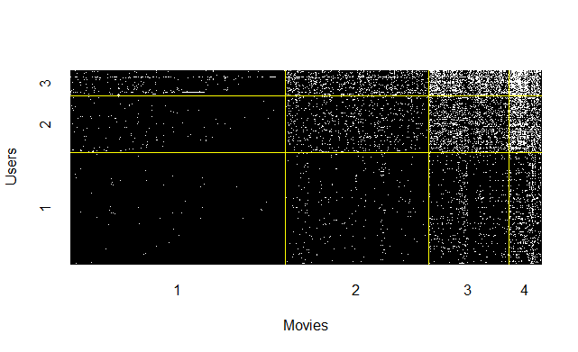
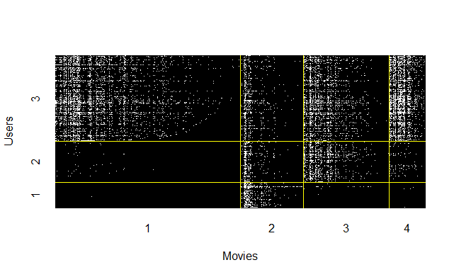
Figure 4: Heatmaps on the MovieLens matrix $A$ with rows and columns rearranged by biclustering results. White pixels: $A_{ij}=1$. Black pixels: $A_{ij}=0$. Yellow lines: boundaries of estimated clusters. PL: profile likelihood based biclustering.

(a) User clusters by PL (b) Movie clusters by PL

(c) User clusters by DC-LBM (d) Movie clusters by DC-LBM

Figure 5: Histograms of of degrees in user and movie clusters identified by PL and DC-LBM, respectively. PL: profile likelihood based biclustering.

Furthermore, we compare the frequencies of degrees in user and movie clusters identified by profile likelihood based biclustering and DC-LBM in Figure 5. As in the histograms, the degrees are much more homogeneous within a user or a movie cluster found by profile likelihood based biclustering than in the clusters found by DC-LBM, which is in line with the observation from Figure 4.

Finally, we study whether the estimated movie clusters are associated with the true movie categories provided in the MovieLens dataset. The 1682 movies in the dataset were labeled with 19 categories such as “Action” or “Romance” and many of the movies belong to multiple categories. A direct comparison between the estimated clusters and the true categories is difficult due to the relatively large number of movie categories and the overlaps. We instead construct contingency tables with row categories being the estimated movie clusters and column categories being the ground truth and evaluate how much the table deviates from an independence model. Specifically, we filtered the data to only include movies belonging to a single category, resulting 833 movies, and constructed contingency tables for profile likelihood based biclustering and DC-LBM, respectively. We then ran the chi-squared test of independence on the two tables. The p-values for the tables constructed from clusters estimated by profile likelihood based biclustering and DC-LBM are $0.0415$ and $2.656\times 10^{-7}$, respectively, which suggests that the movie clusters estimated by DC-LBM have a stronger association with the true movie categories.

7 Discussion

We discuss related theoretical work. Zhao et al., (2012) proved a general theorem for label consistency under the DC-SBM with degree parameters taking a finite number of possible values. Amini et al., (2013); Wang et al., 2021a ; Wang et al., 2021b considered the DC-SBM but the theoretical analyzes focused on the classical SBM. Spectral clustering (Rohe et al.,, 2011; Lei and Rinaldo,, 2015; Jin,, 2015; Wang et al., 2021c, ) provides a fast non-likelihood-based approach for community detection. Mariadassou et al., (2015) proposed a unified framework for studying the convergence of the posterior distribution of cluster labels under both the SBM and LBM with known parameter values.

There are a number of directions for future work. It would be interesting to consider the selection of the number of clusters for bipartite networks. Recently, a number of likelihood-based model selection methods have been proposed for the SBM (Saldana et al.,, 2017; Wang and Bickel,, 2017; Hu et al.,, 2020), most of which cannot directly be applied to bipartite graphs. We would also like to consider the generalization of DC-LBM into other clustering problems in the context of bipartite networks, such as estimating mixed memberships (Airoldi et al.,, 2008; Jin et al.,, 2017) and incorporating node features (Zhang et al.,, 2016; Zhao et al.,, 2019).

References

• Abbe, (2017) Abbe, E. (2017). Community detection and stochastic block models: recent developments. The Journal of Machine Learning Research, 18(1):6446–6531.
• Airoldi et al., (2008) Airoldi, E. M., Blei, D. M., Fienberg, S. E., and Xing, E. P. (2008). Mixed membership stochastic blockmodels. J. Machine Learning Research, 9:1981–2014.
• Alqadah et al., (2015) Alqadah, F., Reddy, C. K., Hu, J., and Alqadah, H. F. (2015). Biclustering neighborhood-based collaborative filtering method for top-n recommender systems. Knowledge and Information Systems, 44(2):475–491.
• Amini et al., (2013) Amini, A. A., Chen, A., Bickel, P. J., Levina, E., et al. (2013). Pseudo-likelihood methods for community detection in large sparse networks. The Annals of Statistics, 41(4):2097–2122.
• Bickel et al., (2013) Bickel, P., Choi, D., Chang, X., and Zhang, H. (2013). Asymptotic normality of maximum likelihood and its variational approximation for stochastic blockmodels. The Annals of Statistics, 41(4):1922–1943.
• Bickel and Chen, (2009) Bickel, P. J. and Chen, A. (2009). A nonparametric view of network models and Newman-Girvan and other modularities. Proc. Natl. Acad. Sci. USA, 106:21068–21073.
• Brault et al., (2020) Brault, V., Keribin, C., and Mariadassou, M. (2020). Consistency and asymptotic normality of latent block model estimators. Electronic journal of statistics, 14(1):1234–1268.
• Celeux and Govaert, (1991) Celeux, G. and Govaert, G. (1991). Clustering criteria for discrete data and latent class models. Journal of classification, 8(2):157–176.
• Cheng and Church, (2000) Cheng, Y. and Church, G. M. (2000). Biclustering of expression data. In Ismb, volume 8, pages 93–103.
• Daudin et al., (2008) Daudin, J.-J., Picard, F., and Robin, S. (2008). A mixture model for random graphs. Statistics and computing, 18(2):173–183.
• de Castro et al., (2007) de Castro, P. A., de França, F. O., Ferreira, H. M., and Von Zuben, F. J. (2007). Applying biclustering to text mining: an immune-inspired approach. In International Conference on Artificial Immune Systems, pages 83–94. Springer.
• Flynn and Perry, (2020) Flynn, C. and Perry, P. (2020). Profile likelihood biclustering. Electronic Journal of Statistics, 14(1):731–768.
• Fraley and Raftery, (2002) Fraley, C. and Raftery, A. E. (2002). Model-based clustering, discriminant analysis, and density estimation. Journal of the American statistical Association, 97(458):611–631.
• Govaert and Nadif, (2003) Govaert, G. and Nadif, M. (2003). Clustering with block mixture models. Pattern Recognition, 36(2):463–473.
• Govaert and Nadif, (2006) Govaert, G. and Nadif, M. (2006). Fuzzy clustering to estimate the parameters of block mixture models. Soft Computing, 10(5):415–422.
• Govaert and Nadif, (2008) Govaert, G. and Nadif, M. (2008). Block clustering with bernoulli mixture models: Comparison of different approaches. Computational Statistics & Data Analysis, 52(6):3233–3245.
• Harper and Konstan, (2015) Harper, F. M. and Konstan, J. A. (2015). The movielens datasets: History and context. Acm transactions on interactive intelligent systems (tiis), 5(4):1–19.
• Hartigan, (1972) Hartigan, J. A. (1972). Direct clustering of a data matrix. Journal of the american statistical association, 67(337):123–129.
• Holland et al., (1983) Holland, P. W., Laskey, K. B., and Leinhardt, S. (1983). Stochastic blockmodels: first steps. Social Networks, 5(2):109–137.
• Hu et al., (2020) Hu, J., Qin, H., Yan, T., and Zhao, Y. (2020). Corrected bayesian information criterion for stochastic block models. Journal of the American Statistical Association, 115(532):1771–1783.
• Jin, (2015) Jin, J. (2015). Fast community detection by score. The Annals of Statistics, 43(1):57–89.
• Jin et al., (2017) Jin, J., Ke, Z. T., and Luo, S. (2017). Estimating network memberships by simplex vertex hunting. arXiv preprint arXiv:1708.07852.
• Karrer and Newman, (2011) Karrer, B. and Newman, M. E. J. (2011). Stochastic blockmodels and community structure in networks. Physical Review E, 83:016107.
• Kernighan and Lin, (1970) Kernighan, B. W. and Lin, S. (1970). An efficient heuristic procedure for partitioning graphs. The Bell system technical journal, 49(2):291–307.
• Lei and Rinaldo, (2015) Lei, J. and Rinaldo, A. (2015). Consistency of spectral clustering in stochastic block models. The Annals of Statistics, 43(1):215–237.
• Mariadassou et al., (2015) Mariadassou, M., Matias, C., et al. (2015). Convergence of the groups posterior distribution in latent or stochastic block models. Bernoulli, 21(1):537–573.
• Ng et al., (2002) Ng, A. Y., Jordan, M. I., and Weiss, Y. (2002). On spectral clustering: Analysis and an algorithm. In Advances in neural information processing systems, pages 849–856.
• Orzechowski and Boryczko, (2016) Orzechowski, P. and Boryczko, K. (2016). Text mining with hybrid biclustering algorithms. In International Conference on Artificial Intelligence and Soft Computing, pages 102–113. Springer.
• Pontes et al., (2015) Pontes, B., Giráldez, R., and Aguilar-Ruiz, J. S. (2015). Biclustering on expression data: A review. Journal of biomedical informatics, 57:163–180.
• Rohe et al., (2011) Rohe, K., Chatterjee, S., and Yu, B. (2011). Spectral clustering and the high-dimensional stochastic block model. Annals of Statistics, 39(4):1878–1915.
• Saldana et al., (2017) Saldana, D. F., Yu, Y., and Feng, Y. (2017). How many communities are there? Journal of Computational and Graphical Statistics, 26(1):171–181.
• Vinh et al., (2010) Vinh, N. X., Epps, J., and Bailey, J. (2010). Information theoretic measures for clusterings comparison: Variants, properties, normalization and correction for chance. The Journal of Machine Learning Research, 11:2837–2854.
• (33) Wang, J., Liu, B., and Guo, J. (2021a). Efficient split likelihood-based method for community detection of large-scale networks. Stat, 10(1):e349.
• (34) Wang, J., Zhang, J., Liu, B., Zhu, J., and Guo, J. (2021b). Fast network community detection with profile-pseudo likelihood methods. Journal of the American Statistical Association, (just-accepted):1–32.
• Wang and Bickel, (2017) Wang, Y. R. and Bickel, P. J. (2017). Likelihood-based model selection for stochastic block models. The Annals of Statistics, 45(2):500–528.
• (36) Wang, Z., Liang, Y., and Ji, P. (2021c). Spectral algorithms for community detection in directed networks. Journal of Machine Learning Research, 21:1–45.
• Zhang et al., (2016) Zhang, Y., Levina, E., and Zhu, J. (2016). Community detection in networks with node features. Electronic Journal of Statistics, 10(2):3153–3178.
• Zhao, (2017) Zhao, Y. (2017). A survey on theoretical advances of community detection in networks. Wiley Interdisciplinary Reviews: Computational Statistics, 9(5).
• Zhao et al., (2012) Zhao, Y., Levina, E., and Zhu, J. (2012). Consistency of community detection in networks under degree-corrected stochastic block models. The Annals of Statistics, 40(4):2266–2292.
• Zhao et al., (2019) Zhao, Y., Pan, Q., and Du, C. (2019). Logistic regression augmented community detection for network data with application in identifying autism-related gene pathways. Biometrics, 75(1):222–234.