GOOD: A Graph Out-of-Distribution Benchmark

Abstract

Out-of-distribution (OOD) learning deals with scenarios in which training and test data follow different distributions. Although general OOD problems have been intensively studied in machine learning, graph OOD is only an emerging area of research. Currently, there lacks a systematic benchmark tailored to graph OOD method evaluation. In this work, we aim at developing an OOD benchmark, known as GOOD, for graphs specifically. We explicitly make distinctions between covariate and concept shifts and design data splits that accurately reflect different shifts. We consider both graph and node prediction tasks as there are key differences in designing shifts. Overall, GOOD contains 11 datasets with 17 domain selections. When combined with covariate, concept, and no shifts, we obtain 51 different splits. We provide performance results on 10 commonly used baseline methods with 10 random runs. This results in 510 dataset-model combinations in total. Our results show significant performance gaps between in-distribution and OOD settings. Our results also shed light on different performance trends between covariate and concept shifts by different methods. Our GOOD benchmark is a growing project and expects to expand in both quantity and variety of resources as the area develops. The GOOD benchmark can be accessed via https://github.com/divelab/GOOD/.

1 Introduction

In machine learning, training and test data are commonly assumed to be i.i.d.. Models designed under this assumption may not perform well when the i.i.d. assumption does not hold. The area of out-of-distribution (OOD) learning deals with scenarios in which training and test data follow different distributions. Two commonly studied OOD settings are covariate shift and concept shift. Over the years, multiple OOD methods have been proposed [12, 44, 3, 41, 25]. To facilitate evaluations, several benchmarks have been curated, including DomainBed [17], OoD-Bench [53], and WILDS [24]. Although both general OOD problems and graph analysis [23, 13, 46, 52, 30] have been intensively studied, graph OOD is only an emerging area of research [50, 49, 60, 6]. Some initial attempts have been made to curate graph OOD benchmarks [21, 9]. However, existing benchmarks lack in several aspects, as detailed in Section 2.

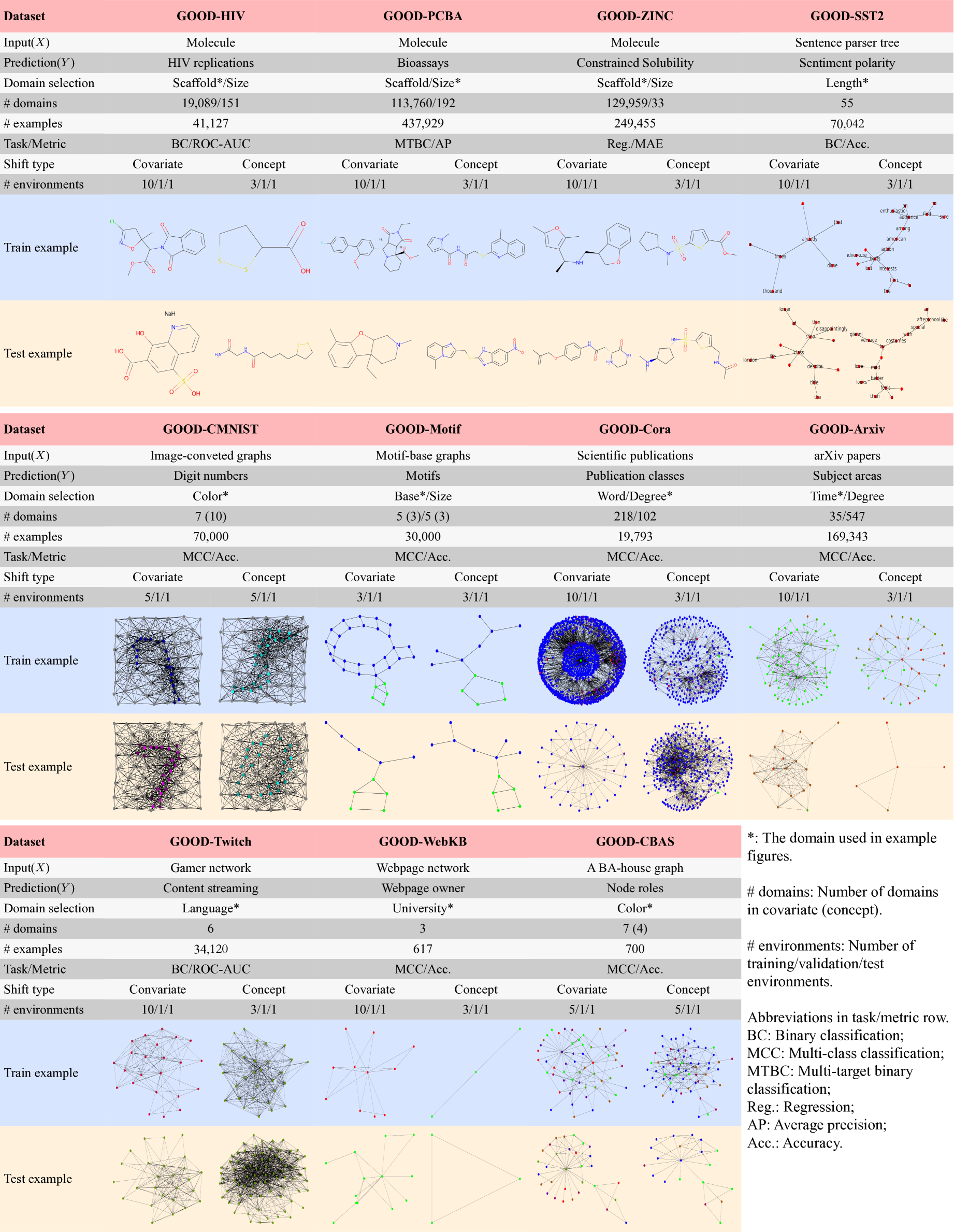
Figure 1: A summary of datasets included in the proposed benchmark. For a covariate shift, the training and test examples are from different domains. For a concept shift, examples are chosen from the same domain with different labels to show the different domain-output correlations.

Covariate shift and concept shift. Distribution shifts can generally be defined as two types; i.e., covariate shift and concept shift (drift) [39, 36, 48]. Formally, in supervised learning, a model is trained to predict an output $Y\in\mathcal{Y}$ given an input $X\in\mathcal{X}$, also known as a covariate variable. The output $Y$ is categorical in classification and continuous in regression problems. In multi-task learning, the output $Y$ becomes a vector, and we consider each task separately. Since the joint distribution $P(Y,X)$ can be written as $P(Y|X)P(X)$, two types of OOD problems are commonly considered, namely covariate and concept shifts. In covariate shift, the input distributions have been shifted between training and test data. Formally, $P^{\text{train}}(X)\neq P^{\text{test}}(X)$ and $P^{\text{train}}(Y|X)=P^{\text{test}}(Y|X)$, where $P^{\text{train}}(\cdot)$ and $P^{\text{test}}(\cdot)$ denote training and test distributions, respectively. In contrast, in concept shift, the conditional distribution $P(Y|X)$ has been shifted as $P^{\text{train}}(Y|X)\neq P^{\text{test}}(Y|X)$ and $P^{\text{train}}(X)=P^{\text{test}}(X)$. In this work, we explicitly make distinctions and consider both shifts.

Differences between graph OOD and general OOD. Traditional OOD methods commonly focus on simple structure equation models [3, 1, 40, 33] or computer vision tasks [33, 45, 12, 44]. In these tasks, the inputs are variables or image features, denoted as $F$. However, graph data possess the complex nature of irregularity and connectivity in topology. A graph is commonly represented as an input pair $(F,A)$, where $F$ are node/edge features, and $A$ is the adjacency matrix. Consequently, graph OOD problems focus not only on general feature distribution shifts but also on structure distribution shifts. Graph neural networks are designed based on $F$ and $A$ to pass messages, demonstrating that structures and features carry different perspectives of input information of a graph. The uniqueness of graph data prompts the development of graph-specific OOD methods [50, 49, 6, 60, 10, 27] and calls for graph OOD benchmarks.

Contributions and novelty. In this work, we develop a systematic graph OOD benchmark, known as GOOD. As design principles, we strive to (1) create non-trivial performance gaps between training and test data; and (2) provide carefully designed data environments to ensure that the induced distribution shifts are potentially solvable for models. Specifically, GOOD contains 6 graph-level datasets and 5 node-level datasets as shown in Fig. 1. For each dataset, we select one or two types of domains. Given a domain, we generate no-shift, covariate shift, and concept shift splits for ease of comparison among 10 baselines. We summarize our novel contributions as follows. (1) To the best of our knowledge, no existing OOD benchmark provides both covariate and concept shifts comparison for the same domain selection. This is important as it sheds light on the differences between various shifts with proper variable control. For example, from our experiments, DIR [50] performs favorably against other methods in concept shift of GOOD-HIV size split while failing in the corresponding covariate shift. (2) In terms of graph OOD, we are the first benchmark to include not only graph classification, but also graph regression and node-level datasets, which improves the diversity of graph OOD tasks. (3) GOOD provides numerous comparisons for 51 different dataset splits and 10 OOD methods, providing solid baselines for future method developments.

2 Related Work

OOD or distribution shift is a longstanding problem in machine learning and artificial intelligence [18, 39, 36, 42]. To address OOD problem substantially, several benchmarks have been curated [17, 53, 19, 24, 58] to evaluate different algorithms [12, 44, 38, 3, 25, 41, 57, 1]. DomainBed [17] is an early OOD benchmark in computer vision. Following DomainBed, OoD-Bench [53] collects datasets and categorizes them into diversity and correlation shifts. WILDS [24] collects real-world data from wild and studies domain generalization and subpopulation shift. Specifically, domain generalization focuses on disjoint training and test domains, while subpopulation shift considers shifts between majority and minority groups, which leads to insufficient training for minority data. With the success of graph neural networks [23, 52, 46, 13, 29, 14, 31, 32], graph OOD problems are gaining growing attention [50, 49, 6, 60, 10, 27, 28, 8]. GDS [9] collects several datasets to compare the performance of well-known baselines and data augmentation methods. DrugOOD [21] is a recent benchmark specifically designed for molecular graph OOD problems. It is curated based on a large-scale bioassay dataset ChEMBL [34] and includes an automated pipeline for obtaining more datasets.

Differences with existing (graph) OOD benchmarks. Generalization abilities of OOD algorithms for covariate shift [43] and concept shift [48, 18, 2, 25] differ fundamentally. However, existing benchmarks, including but not limited to graph OOD benchmarks, either ignore one of the shifts or fail to compare the two shifts of the same feature on the same dataset. Firstly, most existing OOD benchmarks include only one type of shift. For example, DrugOOD [21] focuses on domain generalization for molecules, exclusively considering covariate shift. WILDS [24] includes domain generalization and subpopulation shift, which are two cases of covariate shift, while still ignoring concept shift. Secondly, a few benchmarks [53] involve both shifts but simply categorize each dataset as one of these two shifts. GDS [9] collects eight datasets but makes no distinctions between the two shifts; among their datasets, we can categorize ColoredMNIST as concept shift and others as covariate shift. In contrast, our benchmark proposes novel dataset splitting methods to generate both shifts for the same domain selection on the same dataset to enable comparison between shifts. This variable-controlled comparison enables a more thorough analysis of shifts given any specific domain, leading to a more comprehensive OOD benchmark. Furthermore, we curate more diverse graph datasets with diverse tasks, including single/multi-task graph classification, graph regression, and node classification, while neither GDS nor DrugOOD includes graph regression or node-level tasks. In addition, while GDS and DrugOOD do not benchmark any graph-specific OOD methods, we evaluate 4 graph-specific OOD methods, shedding light on further graph OOD research.

3 The GOOD Benchmark Design

When training and test samples are assumed to be i.i.d., random split is commonly used to split datasets into training and test sets. In contrast, splits in OOD problems should be carefully designed in order to accurately assess the generalization ability of algorithms. In GOOD, we consider both covariate and concept shifts and meticulously design data splits to ensure these shifts are reflected. Formally, following prior invariant learning work [3, 8, 1, 40, 33], as shown in Fig. 2(b), $C,S_{1},S_{2}\in\mathcal{Z}$ are the latent variables that causes target $Y\in\mathcal{Y}$, is non-causally associated with $Y$, and is independent to $Y$, respectively. $\rightarrow$ denotes the causal mapping. $S_{2}$ is commonly caused by target-irrelevant environments. In the input feature space, given input features $X\in\mathcal{X}$, we assume the invariant features $X_{\text{inv}}\in X$ are projected by an injective function from $C$. Therefore, $X_{\text{inv}}$ can fully determine $Y$. $X_{\text{ass}}$ denotes input features associated with $Y$ by confounding and anti-causal associations through $C$ and $S_{1}$. $X_{\text{ind}}$ are input features independent to $Y$ and are only caused by $S_{2}$. In practice, it might be hard to strictly separate $X_{\text{inv}}$, $X_{\text{ass}}$, and $X_{\text{ind}}$. We try to only select and shift part of $X_{\text{ind}}$, but since our shift splits contain significant dataset shifts, the selection of parts of $X_{\text{ass}}$ won’t affect the benchmarking performance. Though, we use $X_{\text{ind}}$ throughout this paper for simplicity.

3.1 Covariate shifts

Domain generalization methods follow the covariate shift assumption [5] and assume that the covariate distribution $P(X)$ shifts across splits, while the concept distribution $P(Y|X)$ remains the same. This implies that a shift of $P(X)$ should not cause corresponding shift in $P(Y|X)$. That is, covariate shift can only happen on input features that are not associated with $Y$. Therefore, with prior knowledge, we can manually select and shift one or several of these irrelevant features, $X_{\text{ind}}$, to build covariate splits. Different $X_{\text{ind}}$ feature values indicate different domains, and each domain can be viewed as a split. For instance, in the graph ColoredMNIST dataset in which we distinguish hand-written digits with colors, the color is irrelevant with labels. Thus, in our covariate splits, digits with different colors belong to corresponding color domains, and each domain becomes a split.

Formally, possible values of $X_{\text{ind}}$ are discrete and finite. Therefore, we define each domain by its unique $X_{\text{ind}}$ value, forming its unique input distribution $P(X)$. Then, a dataset can be viewed as a mixture of $|\mathcal{D}|$ domains as $\mathcal{D}=\{d_{1},\ldots,d_{|\mathcal{D}|}\}$. For a domain $d_{i}$, we represent its input distribution as $P_{d_{i}}(X)$. Specifically, $P_{d_{i}}(X_{\text{inv}},X_{\text{ass}})$ is fixed while $P_{d_{i}}(X_{\text{ind}}=\mathbf{x}_{i})=1$, where $\mathbf{x}_{i}$ is the value of $X_{\text{ind}}$ in domain $d_{i}$. Since $X_{\text{ind}}$ is independent to $Y$, $P_{d_{i}}(Y|X)=P(Y|X)$. The data distribution is

$$P(Y,X)=\sum\limits^{|\mathcal{D}|}_{i=1}w_{i}P_{d_{i}}(Y,X)=\sum\limits^{|\mathcal{D}|}_{i=1}w_{i}P_{d_{i}}(X)P(Y|X),$$ (1)

where $w_{i}$ is the mixture weight for domain $d_{i}$.

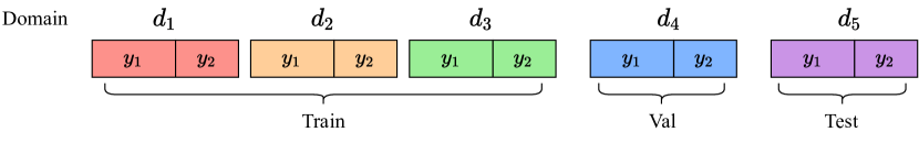
(a) Covariate shift split

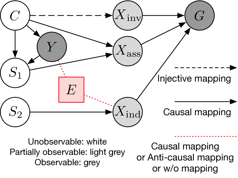
(b) Causal graph

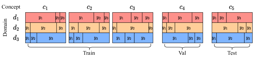
(c) Concept shift split

Figure 2: (a) Illustration of covariate shift split. Five domains are denoted as different colors, where each domain includes outputs of the same distribution. We sort the dataset according to the domain $d_{i}$, then group them into train/validation/test sets. (c) Illustration of concept shift split. Each concept includes all three domains, and each domain has spurious correlations with a specific output in a concept. For example, in concept $c_{1}$, the domain colored in red is highly associated with $y_{1}$, but this domain corresponds to $y_{2}$ in concept $c_{4}$. Note that the distributions of concepts in training are similar. (b) Illustration of causal graph [37, 38] for dataset generation and observation. (Left) $C$, $S_{1}$, $S_{2}$ locate in the latent space and are not observable. (Middle) $X_{\text{inv}}$, $X_{\text{ass}}$, and $X_{\text{ind}}$ are input features that can be partially observed and selected manually, such as motif shapes or molecule scaffolds. (Right) $G$ is the graph data input including node features and adjacency matrices. $E\in\mathcal{E}$ is the environment variable that can determine or be determined by $X_{\text{inv}}$ and $Y$ according to different types of datasets and shifts. Detailed discussions can be found in Appendix A.

Comparison of covariate split design on 3 types of datasets. We perform covariate shift splits on synthetic, semi-artificial, and real-world datasets. For a synthetic dataset, given the $X_{\text{ind}}$ feature values of each domain, we generate graphs according to its domain distributions, respectively. For a semi-artificial dataset, given a graph, we generate extra variant features to produce modified graphs that follow the domain distribution. Since we cannot create or modify graphs for real-world datasets, we use carefully designed data splits. As shown in Fig. 2(a), we sort the graphs by their domain $d_{i}\in\mathcal{D}$ and then divide the dataset into five domain splits with a specific split ratio, e.g., $20\%$, for each domain. Finally, the training, validation, and test sets are obtained based on domains without intersections. The difference between synthetic/semi-artificial datasets and real-world datasets is that the domain of graphs in artificial datasets can be defined arbitrarily before feature modifications, but the domain of graphs in real-world datasets should be defined strictly according to its features.

3.2 Concept shifts

In contrast to covariate shift, concept shift considers the scenario in which the concept distribution $P(Y|X)$ is shifted across splits. Since $X_{\text{inv}}$ can fully determine $Y$, $P(Y|X_{\text{inv}})$ is invariant. Thus, shifts of $P(Y|X)$ can only happen with shifts of $P(Y|X_{\text{ass}})$ and $P(Y|X_{\text{ind}})$. Since $X_{\text{ind}}$ is irrelevant with $Y$, the correlation $P(Y|X_{\text{ind}})$ between $Y$ and $X_{\text{ind}}$ in each domain is spurious correlation. However, the association built between $Y$ and $X_{\text{ind}}$ will also connect $X_{\text{inv}}$ to $X_{\text{ind}}$ through $Y$ according to Fig. 2(b), leading to the change of $P(X_{\text{inv}}|X_{\text{ind}})$, so that $P(X)$ will be changed inevitably. Therefore, we can only build major concept shifts with necessary covariate shifts. We will still call it concept shift for simplicity and distinction. Therefore, given the selected domain features $X_{\text{ind}}$, we can build concept shift splits by manually creating such spurious correlations of certain rates. For example, the spurious correlation rate between the domain $d_{i}$ and the output value $y_{j}$ can be set as $P(Y=y_{j}|X_{\text{ind}}=\mathbf{x}_{i})=90\%$. Specifically, different spurious correlation rates define different concepts, and each concept can be viewed as a split. We use the graph ColoredMNIST dataset as an example, as shown in Fig. 2(c). In every concept, each color domain is highly correlated with a label. Therefore, in our concept splits, different spurious color-label correlation rates determine different concepts, and each concept becomes a split.

Formally, a dataset can be viewed as a mixture of $|\mathcal{C}|$ concepts $\mathcal{C}=\{c_{1},\ldots,c_{|\mathcal{C}|}\}$ in our concept shift split. We use $P_{y_{j},d_{i}}(Y)$ to represent a certain output distribution on value $y_{j}$ given domain $d_{i}$, defined as $P(Y=y_{j}|X_{\text{ind}}=\mathbf{x_{i}})=1$. We first consider the classification case in which $Y$ is categorical. Given a concept ${c_{k}}$, we formulate its 2-D conditional distribution $P_{c_{k}}(Y|X)$ by describing multiple 1-D distributions; that is, for each domain $d_{i}$,

$$P_{c_{k}}(Y|X_{\text{ind}}=\mathbf{x_{i}})=\sum\limits^{|\mathcal{Y}|}_{j=1}q_{i,j}^{k}P_{y_{j},d_{i}}(Y),$$ (2)

where $q_{i,j}^{k}$ is the rate of the spurious correlation in concept ${c_{k}}$ between domain $d_{i}$ and output $y_{j}$. In the regression case where $Y$ is continuous, the sum becomes integral. In the multi-task case, $Y$ and $y_{j}$ become vectors. The overall dataset distribution can be written as

$$P(Y,X)=\sum\limits_{k=1}^{|\mathcal{C}|}w_{k}P_{c_{k}}(Y,X)=\sum\limits_{k=1}^{|\mathcal{C}|}w_{k}P(X)_{c_{k}}P_{c_{k}}(Y|X),$$ (3)

where $w_{k}$ is the mixture weight for concept $c_{k}$.

Comparisons of concept split design on 3 types of datasets. In practice, we create significant concept shifts between training, validation, and test sets, in which the domain-output correlations are completely different. Note that mixing different domain-output correlations can weaken the spuriousness of these correlations. Thus, concepts within the training set are designed to have similar domain-output correlations to guarantee the concept shift between training and test. Concretely, we perform concept shift splits on synthetic, semi-artificial, and real-world datasets. For synthetic datasets, we generate graphs where the domain feature is highly correlated with a specific output according to the preset correlation in the concept. For semi-artificial datasets, given a graph and a concept, we generate extra features as domains to build spurious domain-output correlations. For real-world datasets, we cannot create or modify data. Thus, we propose a screening approach to scan and select graphs in the dataset. Each graph has a probability to be included in a concept $c_{k}$ according to the value of $q_{i,j}^{k}$. To conclude, the difference in concept splits between artificial datasets and real-world datasets is located in whether we can arbitrarily determine the concept of a graph. We can define the concept of a graph in artificial datasets, but the concept of a graph in real-world datasets is defined with a probability according to $X_{\text{ind}}$ and target $Y$.

3.3 Environments

Many current OOD learning algorithms [41, 25] follow the framework of invariant causal predictor (ICP) [38] and invariant risk minimization (IRM) [3], assuming that the training data form groups by distributions, known as environments. This framework assumes the data are similar within an environment and dissimilar across different environments. Since OOD problems are complicated and multi-perspective, works under this framework explicitly or implicitly injects environment information to models to figure out the specific generalization direction for better OOD performances. Specifically, the shift between training and test data, though more significant, should be similarly reflected among different training environments, so that OOD models can potentially grasp the shift between training and test data by learning the shifts among different training environments. Following this strategy, to enhance the OOD generalization ability of models, we use the distribution shift information provided by the difference of training environments to convey the types of shifts expected between training and test data. In covariate shift, environments take the form of domains. During training, models can learn from $P^{\text{train}}(X_{\text{ind}})$, which varies across domains, that $X_{\text{ind}}$ is not causally related to labels, thereby preventing the unknown $P^{\text{test}}(X_{\text{ind}})$ from misleading predictions during test. In concept shifts, environments take the form of concepts. By learning from different spurious correlations across training concepts, models can learn that the domain-output correlations $P^{\text{train}}(Y|X_{\text{ind}})$ are spurious, thereby avoiding being misled by the new spurious correlation $P^{\text{test}}(Y|X_{\text{ind}})$ during test.

Formally, we consider a dataset with a set of $|\mathcal{E}|$ environments $\mathcal{E}=\{e_{1},\ldots,e_{|\mathcal{E}|}\}$, each with distribution $P_{e}(Y,X)$ for $e\in\mathcal{E}$ (Fig 2(b)). In this case, the dataset distribution $P(Y,X)=\sum_{e}P_{e}(Y,X)$. Specifically, for both covariate and concept shifts, the distributions $P^{\text{train}}$ and $P^{\text{test}}$ are weighted combinations of environment distributions $P_{e}(Y,X)$. With the training and test environments $\mathcal{E}^{\text{train}},\mathcal{E}^{\text{test}}\subset\mathcal{E}$, we express $P\textsuperscript{train}=\sum_{e\in\mathcal{E}^{\text{train}}}w_{e}^{\text{train}}P_{e}(Y,X)$ and $P\textsuperscript{test}=\sum_{e\in\mathcal{E}^{\text{test}}}w_{e}^{\text{test}}P_{e}(Y,X)$, where $w_{e}^{\text{train}}$ and $w_{e}^{\text{test}}$ are the weights for each training and test environment, respectively.

4 The GOOD Datasets

In this section, we introduce the datasets in GOOD. The benchmark contains 11 datasets, covering multiple tasks and data sources. For each dataset, we select one or two domain features. Then we apply covariate and concept shift splits per domain to create diverse distribution shifts between training, OOD validation, and OOD test sets. Finally, we shuffle the training set and divide it into final training set, in-domain (ID) validation set, and in-domain (ID) test set. Summary statistics of datasets are given in Fig. 1. Other details and data processing details are included in Appendix A.

4.1 Graph prediction tasks

GOOD-HIV is a small-scale real-world molecular dataset adapted from MoleculeNet [51]. The inputs are molecular graphs in which nodes are atoms, and edges are chemical bonds. The task is to predict whether the molecule can inhibit HIV replication. We design splits based on two domain selections, namely, scaffold and size. The first one is Bemis-Murcko scaffold [4] which is the two-dimensional structural base of a molecule. The second one is the number of nodes in a molecular graph, an inevitable structural feature of a graph. Both features should not determine the label, therefore, both can become major sources of distribution shifts. For each domain selection, the value space for the feature is very large, therefore we cluster graphs with similar domain values into one environment, improving the OOD learning procedure and reducing the training time complexity.

GOOD-PCBA is a real-world molecular dataset from Wu et al. [51]. It includes 128 bioassays, forming 128 binary classification tasks. Due to the extremely unbalanced classes (only 1.4% positive labels), we use the Average Precision (AP) averaged over the tasks as the evaluation metric. GOOD-PCBA uses the same domain selections as GOOD-HIV.

GOOD-ZINC is a real-world molecular property regression dataset from ZINC database [16]. The inputs are molecular graphs with up to 38 heavy atoms, and the task is to predict the constrained solubility [22, 26] of molecules. GOOD-ZINC uses the same domain selections as GOOD-HIV.

GOOD-SST2 is a real-world natural language sentimental analysis dataset adapted from Yuan et al. [55]. Each sentence is transformed into a grammar tree graph, where each node represents a word with corresponding word embeddings as node features. The dataset forms a binary classification task to predict the sentiment polarity of a sentence. We select sentence lengths as domains since the length of a sentence should not affect the sentimental polarity.

GOOD-CMNIST is a semi-artificial dataset designed for node feature shifts. It contains graphs of hand-written digits transformed from MNIST database using superpixel techniques [35]. Following Arjovsky et al. [3], we color digits according to their domains and concepts. Specifically, in covariate shift split, we color digits with 7 different colors, and digits with the first 5 colors, the 6th color, and the 7th color are categorized into training, validation, and test sets. In concept shift split, we color digits with 10 colors. Each color is highly correlated with one digit label in the training set, while colors have weak correlations and no correlation with labels in validation and test sets, respectively.

GOOD-Motif is a synthetic dataset motivated by Spurious-Motif [50] and is designed for structure shifts. Particularly, GOOD-CMNIST and GOOD-Motif compose an OOD algorithm check for both feature/structure shifts. Each graph in the dataset is generated by connecting a base graph and a motif, and the label is determined by the motif solely. Instead of combining the base-label spurious correlations and size covariate shift together as in Wu et al. [50], we study covariate and concept shifts separately. Specifically, we generate graphs using five label irrelevant base graphs (wheel, tree, ladder, star, and path) and three label determining motifs (house, cycle, and crane). To create covariate and concept splits, we select the base graph type and the size as domain features.

4.2 Node prediction tasks

GOOD-Cora is a citation network adapted from the full Cora dataset [7]. The input is a small-scale citation network graph, in which nodes represent scientific publications and edges are citation links. The task is a 70-class classification of publication types. We generate splits based on two domain selections, namely, word and degree. The first one is the word diversity defined by the selected-word-count of a publication, purely irrelevant with the label. The second one is node degree in the graph, implying that the popularity of a paper should not determine the class of a paper.

GOOD-Arxiv is a citation dataset adapted from OGB [20]. The input is a directed graph representing the citation network among the computer science (CS) arXiv papers. Nodes in the graph represent arXiv papers, and directed edges represent citations. The task is predicting the subject area of arXiv CS papers, forming a 40-class classification problem. We generate splits based on two domain selections; i.e., time (publication year) and node degree.

GOOD-Twitch is a gamer network dataset. The nodes represent gamers with games as node features, and the edge represents the friendship connection of gamers. The binary classification task is to predict whether a user streams mature content. The domain of GOOD-Twitch splits includes user language, implying that the prediction target should not be biased by the language a user uses.

GOOD-WebKB is a university webpage network dataset. A node in the network represents a webpage, with words appearing in the webpage as node features, and edges are hyperlinks between webpages. Its 5-class prediction task is to predict the classes of webpages. We split GOOD-WebKB according to the domain university, suggesting that classified webpages are based on word contents and link connections instead of university features.

GOOD-CBAS is a synthetic dataset modified from BA-Shapes [54]. The input is a graph created by attaching 80 house-like motifs to a 300-node Barabási–Albert base graph, and the task is to predict the role of nodes, including the top/middle/bottom node of a house-like motif or the node from the base graph, forming a 4-class classification task. Instead of using constant node features, we generate colored features as in GOOD-CMNIST so that OOD algorithms need to tackle node color differences in covariate splits and color-label correlations in concept splits.

5 Experimental Studies

We conduct experiments on 11 datasets with 10 baseline methods. For each dataset, we use the same GNN backbone for all baseline methods for fair comparisons. Specifically, we use GIN-Virtual [52, 15] and GCN [23, 56] as GNN backbones for graph and node prediction tasks, respectively. Note that for GOOD-Motif, we adopt GIN [52] as the GNN backbone since adding virtual nodes does not improve the performance. For all experiments, we select the best checkpoints for ID and OOD tests according to results on ID and OOD validation sets, respectively. Experimental details and hyper-parameter selections are provided in Appendix B. All the datasets, implementation codes, and best checkpoints to reproduce the results in this paper are available at https://github.com/divelab/GOOD/.

5.1 In-distribution versus out-of-distribution performance gap

As introduced in Sec. 1, one principle for designing GOOD is to create non-trivial distribution shifts and performance gaps between training and test data. Equivalently, we expect distinct performance gaps between ID and OOD settings. To verify performance gaps, we run experiments using empirical risk minimization (ERM) and summarize the results in Table 1. The differences between ID_ID and OOD_ID or OOD_OODfor each domain selection and distribution shift show the substantial and consistent performance gap between the ID and OOD settings. In addition, for most splits, OOD_OOD is better than OOD_ID. This implies that OOD validation sets outperform ID validation sets in selecting models with better generalization ability.

			domain selection 1							domain selection 2
			covariate			concept			no-shift	covariate			concept			no-shift
			IDID	OODID	OODOOD	IDID	OODID	OODOOD	IDID	IDID	OODID	OODOOD	IDID	OODID	OODOOD	IDID
GOOD-HIV↑			82.79	68.86	69.58	84.22	65.31	72.33	80.86	83.72	58.41	59.94	88.05	44.75	63.26	80.86
GOOD-PCBA↑			33.45	16.87	16.89	25.95	21.34	21.63	33.77	34.31	17.81	17.86	32.54	14.83	15.36	33.77
GOOD-ZINC↓			0.1224	0.1825	0.1995	0.1222	0.1328	0.1306	0.1233	0.1199	0.2569	0.2427	0.1315	0.1418	0.1403	0.1233
GOOD-SST2↑			89.82	77.76	81.30	94.43	67.26	72.43	91.61	–	–	–	–	–	–	–
GOOD-CMNIST↑			77.96	26.90	28.60	90.00	40.80	42.87	77.30	–	–	–	–	–	–	–
GOOD-Motif↑			92.60	69.97	68.66	92.02	80.87	81.44	92.09	92.28	51.28	51.74	91.73	69.41	70.75	92.09
GOOD-Cora↑			70.43	64.44	64.86	66.05	64.20	64.60	69.41	72.27	55.76	56.30	68.71	60.38	60.54	69.42
GOOD-Arxiv↑			72.69	70.64	71.08	74.76	65.70	67.32	73.02	77.47	58.53	58.91	75.27	61.77	62.99	72.99
GOOD-Twitch↑			70.66	47.73	48.95	80.29	48.57	57.32	68.05	–	–	–	–	–	–	–
GOOD-WebKB↑			38.25	11.64	14.29	65.00	24.77	27.83	47.85	–	–	–	–	–	–	–
GOOD-CBAS↑			89.29	77.57	76.00	89.79	82.22	82.36	99.43	–	–	–	–	–	–	–

Table 1: ID and OOD performance gaps learned with ERM across 51 splits. The metric and domain selections for each dataset are in Fig. 1. ↑ indicates higher values correspond to better performance while ↓ indicates lower for better. ID test results with ID validations are denoted as ID_ID, while OOD test results with ID/OOD validations are written as OOD_ID and OOD_OOD, respectively. Note that the no-shift random split only has the ID setting. We report the average values over 10 runs. The standard deviations are listed in Appendix D.

5.2 Performance of baseline algorithms

In our benchmark, we conduct experiments with 10 baseline methods. Based on the comparison results, we provide an analysis of the learning strategy of OOD methods.

covariate			GOOD-HIV↑				GOOD-PCBA↑				GOOD-ZINC↓				GOOD-CMNIST↑		graph
			scaffold		size		scaffold		size		scaffold		size		color
			IDID	OODOOD	IDID	OODOOD	IDID	OODOOD	IDID	OODOOD	IDID	OODOOD	IDID	OODOOD	IDID	OODOOD
ERM			82.79	69.58	83.72	59.94	33.45	16.89	34.31	17.86	0.1224	0.1995	0.1199	0.2427	77.96	28.60
IRM			81.35	67.97	81.33	59.00	33.56	16.90	34.28	18.05	0.1213	0.2025	0.1222	0.2403	77.92	27.83
VREx			82.11	70.77	83.47	58.53	33.88	16.98	34.09	17.79	0.1211	0.2094	0.1234	0.2384	77.98	28.48
GroupDRO			82.60	70.64	83.79	58.98	33.81	16.98	33.95	17.59	0.1168	0.1934	0.1180	0.2423	77.98	29.07
DANN			81.18	70.63	83.90	58.68	33.63	16.90	34.17	17.86	0.1186	0.2004	0.1188	0.2439	78.00	29.14
Deep Coral			82.53	68.61	84.70	60.11	33.47	16.93	34.49	17.94	0.1185	0.2036	0.1134	0.2505	78.64	29.05
Mixup			82.29	68.88	83.16	59.03	30.22	16.59	30.63	17.06	0.1279	0.2240	0.1255	0.2748	77.40	26.47
DIR			82.54	67.47	80.46	57.11	32.55	14.98	32.89	16.61	0.3799	0.6493	0.1541	0.5482	31.09	20.60
covariate			GOOD-Motif↑				GOOD-SST2↑			concept	GOOD-Motif↑				GOOD-SST2↑		graph
			base		size		length				base		size		length
			IDID	OODOOD	IDID	OODOOD	IDID	OODOOD			IDID	OODOOD	IDID	OODOOD	IDID	OODOOD
ERM			92.60	68.66	92.28	51.74	89.82	81.30		ERM	92.02	81.44	91.73	70.75	94.43	72.43
IRM			92.60	70.65	92.18	51.41	89.41	79.91		IRM	92.00	80.71	91.68	69.77	94.10	77.47
VREx			92.60	71.47	92.25	52.67	89.51	80.64		VREx	92.05	81.56	91.67	70.24	94.26	73.16
GroupDRO			92.61	68.24	92.29	51.95	89.59	81.35		GroupDRO	92.01	81.43	91.67	69.98	94.41	71.86
DANN			92.60	65.47	92.23	51.46	89.60	79.71		DANN	92.02	81.33	91.81	70.72	94.02	76.03
Deep Coral			92.61	68.88	92.22	50.97	89.68	79.81		Deep Coral	92.01	81.37	91.68	70.49	94.25	72.34
Mixup			92.68	70.08	92.02	51.48	89.78	80.88		Mixup	91.89	77.63	91.45	67.81	94.12	73.34
DIR			87.73	61.50	84.53	50.41	84.30	77.65		DIR	91.60	72.14	73.10	56.28	93.71	68.76
concept			GOOD-HIV↑				GOOD-PCBA↑				GOOD-ZINC↓				GOOD-CMNIST↑		graph
			scaffold		size		scaffold		size		scaffold		size		color
			IDID	OODOOD	IDID	OODOOD	IDID	OODOOD	IDID	OODOOD	IDID	OODOOD	IDID	OODOOD	IDID	OODOOD
ERM			84.22	72.33	88.05	63.26	25.95	21.63	32.54	15.36	0.1222	0.1306	0.1315	0.1403	90.00	42.87
IRM			82.89	72.59	88.62	59.90	25.89	21.22	32.99	16.07	0.1225	0.1314	0.1278	0.1368	90.02	42.80
VREx			83.84	72.60	88.28	60.23	26.62	22.02	32.49	15.59	0.1186	0.1270	0.1309	0.1419	89.99	43.31
GroupDRO			83.40	73.64	88.28	61.37	26.32	21.83	33.03	15.99	0.1207	0.1281	0.1251	0.1369	90.02	43.32
DANN			83.87	71.92	87.28	65.27	26.07	21.64	32.74	15.78	0.1172	0.1256	0.1253	0.1339	89.94	43.11
Deep Coral			84.65	72.97	87.88	62.28	26.38	21.95	32.67	16.20	0.1187	0.1279	0.1287	0.1370	89.94	43.16
Mixup			82.36	72.03	87.64	64.87	23.73	19.78	30.23	13.36	0.1353	0.1475	0.1423	0.1522	89.95	40.96
DIR			83.28	69.05	79.19	72.61	25.85	22.20	30.53	16.86	0.3501	0.3865	0.2348	0.2871	86.76	22.69
covariate			GOOD-Cora↑				GOOD-Arxiv↑				GOOD-CBAS↑		GOOD-Twitch↑		GOOD-WebKB↑		node
			word		degree		time		degree		color		language		university
			IDID	OODOOD	IDID	OODOOD	IDID	OODOOD	IDID	OODOOD	IDID	OODOOD	IDID	OODOOD	IDID	OODOOD
ERM			70.43	64.86	72.27	56.30	72.69	71.08	77.47	58.91	89.29	76.00	70.66	48.95	38.25	14.29
IRM			70.27	64.77	72.64	56.28	72.66	71.04	77.50	58.98	91.00	76.00	69.75	47.21	39.34	13.49
VREx			70.47	64.80	72.25	56.30	72.66	71.12	77.49	58.99	91.14	77.14	70.66	48.99	39.34	14.29
GroupDRO			70.41	64.72	72.18	56.29	72.68	71.15	77.46	59.08	90.86	76.14	70.84	47.20	39.89	17.20
DANN			70.66	64.77	72.47	56.10	72.74	71.05	77.51	59.00	90.14	77.57	70.67	48.98	39.89	15.08
Deep Coral			70.47	64.72	72.16	56.35	72.66	71.07	77.48	58.97	91.14	75.86	70.67	49.64	38.25	13.76
Mixup			71.54	65.23	74.57	58.20	72.49	71.34	77.61	57.60	73.57	70.57	71.30	52.27	54.65	17.46
EERM			68.79	61.98	73.32	56.88	OOM	OOM	OOM	OOM	67.62	52.86	73.87	51.34	46.99	24.61
SRGNN			70.27	64.66	71.37	54.78	72.50	70.83	75.96	57.52	77.62	74.29	70.58	47.30	39.89	13.23
concept			GOOD-Cora↑				GOOD-Arxiv↑				GOOD-CBAS↑		GOOD-Twitch↑		GOOD-WebKB↑		node
			word		degree		time		degree		color		language		university
			IDID	OODOOD	IDID	OODOOD	IDID	OODOOD	IDID	OODOOD	IDID	OODOOD	IDID	OODOOD	IDID	OODOOD
ERM			66.05	64.60	68.71	60.54	74.76	67.32	75.27	62.99	89.79	82.36	80.29	57.32	65.00	27.83
IRM			66.09	64.60	68.58	61.23	74.67	67.41	75.23	62.97	90.71	83.21	77.05	59.17	65.56	27.52
VREx			66.00	64.57	68.45	60.58	74.80	67.37	75.19	63.00	89.50	82.86	80.29	57.37	65.00	27.83
GroupDRO			66.17	64.62	68.37	60.65	74.73	67.45	75.19	62.88	90.36	82.00	81.95	60.27	65.00	28.14
DANN			66.16	64.51	68.08	60.78	74.73	67.28	75.25	62.91	89.93	82.50	80.28	57.46	65.00	26.91
Deep Coral			66.13	64.58	68.38	60.58	74.77	67.42	75.16	62.85	89.36	82.64	80.14	56.97	65.00	28.75
Mixup			69.66	64.44	70.32	63.65	74.92	64.84	72.75	61.28	93.64	64.57	78.89	55.28	67.22	31.19
EERM			65.75	63.09	66.50	58.38	OOM	OOM	OOM	OOM	78.33	64.29	83.91	51.94	61.67	27.83
SRGNN			66.45	64.62	68.34	61.08	74.64	67.17	74.83	62.09	88.57	81.43	80.21	56.05	61.67	27.52

Table 2: ID_ID and OOD_OOD performances of 10 baselines on 11 datasets. All numerical results are averages across 3 to 10 random runs. Numbers in bold represent the best results. OOM denotes out of memory. Additional results are in Appendix D. More empirical results and analysis are in Appendix C.

5.2.1 Baseline methods

We consider empirical risk minimization (ERM) and 9 OOD algorithms as baselines, among which 4 are graph-specific methods. Firstly, we choose two domain adaptation algorithms that target minimizing feature discrepancies. DANN [12] adversarially trains the regular classifier and a domain classifier to make features indistinguishable. Deep Coral [44] encourages features in different domains to be similar by minimizing the deviation of covariant matrices from different domains. Furthermore, we adopt two invariant learning baselines following the invariant prediction assumption [38]. IRM [3] searches for data representations that perform well across all environments by penalizing feature distributions that have different optimal linear classifiers for each environment. VREx [25] targets both covariate robustness and the invariant prediction. It specifically reduces the variance of risks in test environments by minimizing the risk variances of training environments. By applying fair optimization, GroupDRO [41] tackles the problem that the distribution minority lacks sufficient training. This method, known as risk interpolation [25], is achieved by explicitly minimizing the loss in the worst training environment. To evaluate the performance of current OOD methods specifically designed for graphs, we include the following 4 graph OOD methods. We incorporate the data augmentation method Mixup [57] following the implementation of Mixup-For-GraphWang et al. [47] designed for graph data, which improves model generalization abilities. DIR [50] selects a subset of graph representations as causal rationales and conducts interventional data augmentation to create multiple distributions. EERM [49] tries to generate environments by a REINFORCE algorithm to maximize loss variance between environments, while its main loss minimization requires adversarially minimizing loss variance. SRGNN [60] aims at converting the biased training data to the given unbiased distribution, performed through a central moment discrepancy regularizer and the kernel mean matching technique by solving a quadratic problem.

5.2.2 Quantitative comparison and analysis

Table 2 shows the OOD_OOD and ID_ID results of 10 baselines for all splits. Most OOD algorithms have comparable performances with ERM, while many OOD algorithms outperform ERM with certain patterns. Specifically, we observe that the risk interpolation (GroupDRO) and extrapolation (VREx) perform favorably against other methods on multiple datasets and shift splits. VREx outperforms other methods on 7 out of 34 OOD splits, evidencing its learning invariance and robustness, especially for covariate shifts in graph prediction tasks. GroupDRO outperforms 8 out of 34 OOD splits, showing its advantage in fair optimization. The two feature discrepancy minimization methods, DANN and Deep Coral, do not perform well enough. DANN outperforms on 4 splits, and it is especially suitable for graph concept shift splits. Deep Coral outperforms on 1 OOD split but usually has advantages on ID tests. Finally, IRM performs similarly to ERM and outperforms on 3 of the OOD results, showing the difficulty of achieving invariant prediction in non-linear settings.

Graph OOD methods make extra effort to interpolate the irregularity and connectivity of graph topology, and certain improvements are achieved. Mixup-For-Graph exclusively excels at node prediction tasks, yielding consistent gains across datasets, which can attribute to its node-specific design [47]. It outperforms 6 out of 14 node-task OOD splits. However, it fails at graph prediction tasks due to the simple graph representation mixup strategy. DIR specifically solves concept shifts for graph classification tasks and outperforms on 3 splits, indicating that interventional augmentation on representations weakens spurious correlations by diversifying the distribution. Its benefit on concept shift does not apply to covariate shifts since DIR only expands the combination of representations without creating new domains; it also fails on regression tasks which require a more delicate learning process. EERM and SRGNN generally have average performances, outperforming only on a few splits. EERM reveals that while environment generation is learnable with REINFORCE, this adversarial training is difficult and needs to be perfected. SRGNN makes use of our OOD validation data to draw the training data closer to an OOD distribution; however, without sufficient generalization, it can seldom perform well in tests since OOD validation data cannot exactly reflect OOD test data. To conclude, while these graph-specific methods apply well to graph topology, other flaws in the methodology design create a performance bottleneck.

6 Discussions

GOOD aims to facilitate the development of graph OOD and general OOD algorithms. Our results and comparisons show that current OOD algorithms can improve generalization abilities, but not significantly. In addition, an algorithm might improve performance on one type of shift, but not both. With these observations, future OOD methods can focus on solving one of covariate and concept shifts to improve the specific generalization ability. The improvement might be achieved by managing well-designed model architectures, optimization schemes, or data augmentation strategies. Moreover, models cannot be expected to solve unknown distribution shifts. Thus, we believe using the given environment information to convey the types of shifts expected during testing is a promising direction.

Our GOOD benchmark is a growing project. We expect to include more methods as the OOD field develops especially graph-specific algorithms and include datasets and domain selections of a larger quantity and variety. In addition, the current benchmark does not consider link prediction tasks [59], which will be added as the project develops.

Appendix A GOOD Dataset Details

GOOD provides 11 datasets with 17 domain selections. For each domain selection, we provide two shift splits and a no shift split, leading to 51 splits. For each covariate/concept shift split, we split data into 5 subsets, namely, training set, in-distribution (ID) validation set, in-distribution (ID) test set, out-of-distribution (OOD) validation set, and out-of-distribution (OOD) test set. For no shift splits, we split data into training, ID validation, and ID test sets. The statistics of splits are listed in Table 3. Meanwhile, the datasets in GOOD consist of 8 real-world datasets, 1 semi-artificial dataset, and 2 synthetic datasets, and we specify the details of splits for each category in the following three paragraphs. The 8 real-world datasets are public datasets [20, 51, 16, 7] and we closely follow the license rules, which are specified in the Appendix F.

Real-world datasets. For covariate shift splits, given a domain selection, we sort the graphs/nodes by their domains and divide the data into a certain number of domains by specifying the split ratio. Then training, validation, and test sets consist of one or several domains. Also the independence between $Y$ and $X_{\text{ind}}$ guarantees that covariate shift design does not contain concept shift theoretically. For concept shift splits, we adopt a screening process to build the splits. We first explain this screening process for graph prediction datasets. Each concept has specific domain-label correlations, which come in the form of a set of domain-label probabilities. Consequently, to build a specific concept, each graph has a domain-label probability to be included in this concept. Therefore, we build each concept by scanning the whole dataset and selecting graphs to be included according to their probabilities. The selected graphs form the current concept and are excluded from the dataset scanning. We repeat this procedure to form each of the concepts sequentially, and the last concept includes all the remaining graphs. Similarly, in node classification tasks, we apply the screening process to nodes instead of graphs. That is, we build node selection masks instead of collecting graphs out of datasets. Note that the selection probabilities are relatively similar for those concepts within the training set, while largely dissimilar between the training, validation, and test sets. Also, it is difficult to specify all domain-label probabilities for tasks like 70-classes classification in GOOD-Cora, and impossible for regression tasks. Therefore, we design to group labels as only two categories, namely high/low labels. Then we can build concept splits in a clear sense. For example, we assign a high probability for domain $d_{i}$ with label $0$ in training concepts, while a high probability for domain $d_{i}$ with label $1$ in test concepts.

Dataset		Shift	Train	ID validation	ID test	OOD validation	OOD test	Train	OOD validation	ID validation	ID test	OOD test
			Scaffold					Size
GOOD-HIV		covariate	24682	4112	4112	4113	4108	26169	4112	4112	2773	3961
		concept	15209	3258	3258	9365	10037	14454	3096	3096	9956	10525
		no shift	24676	8225	8226	-	-	24676	8225	8226	-	-
			Scaffold					Size
GOOD-PCBA		covariate	262764	43792	43792	44019	43562	269990	43792	43792	48430	31925
		concept	159158	34105	34105	90740	119821	150121	32168	32168	108267	115205
		no shift	262757	87586	87586	-	-	262757	87586	87586	-	-
			Scaffold					Size
GOOD-ZINC		covariate	149674	24945	24945	24945	24946	161893	24945	24945	20270	17402
		concept	101867	21828	21828	43539	60393	89418	19161	19161	51409	70306
		no shift	149673	49891	49891	-	-	149673	49891	49891	-	-
			Length
GOOD-SST2		covariate	24744	5301	5301	17206	17490
		concept	27270	5843	5843	15142	15944
		no shift	42025	14008	14009	-	-
			Color
GOOD-CMNIST		covariate	42000	7000	7000	7000	7000
		concept	29400	6300	6300	14000	14000
		no shift	42000	14000	14000	-	-
			Base					Size
GOOD-Motif		covariate	18000	3000	3000	3000	3000	18000	3000	3000	3000	3000
		concept	12600	2700	2700	6000	6000	12600	2700	2700	6000	6000
		no shift	18000	6000	6000	-	-	18000	6000	6000	-	-
			Word					Degree
GOOD-Cora		covariate	9378	1979	1979	3003	3454	8213	1979	1979	3841	3781
		concept	7273	1558	1558	3807	5597	7281	1560	1560	3706	5686
		no shift	11875	3959	3959	-	-	11875	3959	3959	-	-
			Time					Degree
GOOD-Arxiv		covariate	57073	16934	16934	29799	48603	68607	16934	16934	46264	20604
		concept	62083	13303	13303	32560	48094	58619	12561	12561	34222	51380
		no shift	101605	33869	33869	-	-	101605	33869	33869	-	-
			Language
GOOD-Twitch		covariate	14448	3412	3412	6551	6297
		concept	13605	2914	2914	6762	7925
		no shift	13648	10236	10236	-	-
			University
GOOD-WebKB		covariate	244	61	61	125	126
		concept	282	60	60	106	109
		no shift	370	123	124	-	-
			Color
GOOD-CBAS		covariate	420	70	70	70	70
		concept	140	140	140	140	140
		no shift	420	140	140	-	-

Table 3: Numbers of graphs/nodes in training, ID validation, ID test, OOD validation, and OOD test sets for the 11 datasets.

Semi-artificial datasets. For semi-artificial datasets, we firstly define a domain/concept and modify graph attributes according to the assigned domain/concept. Due to the difficulty in modifying graph structures without breaking the semantics of the original graphs, we choose to modify or append the features of nodes in graphs. GOOD currently corporate one semi-artificial dataset GOOD-CMNIST. For GOOD-CMNIST, since the original colors of graphs are in gray-scale, we color graphs by setting node features as 3-channel RGB colors such as red, blue, and cyan. For covariate shift, the training graphs contain 5 color domains, thus forming 5 environments. Other than these 5 colors, the validation and test set graphs are in different colors, respectively. Therefore, in total, we produce 7 different node color features. For concept shift, each digit label is associated with one color, e.g., 0 with red, 1 with green, 2 with blue, etc. Hence we generate 10 different node color features to match the 10-class labels.

Synthetic datasets. For GOOD-Motif, we generate graphs using five label-independent base graphs (wheel, tree, ladder, star, and path) and three label-dependent motifs (house, cycle, and crane). We select the base graph type and the size as domain features to create covariate and concept splits. In the covariate shift splits with base domain, the training set includes graphs with the first three bases, while the validation and the test sets include graphs with base star and path, respectively. In the concept splits with base domain, for 3 different concepts in the training set, each motif is highly correlated to a specific base graph with different correlation rates; i.e., the house-wheel, cycle-tree, and crane-ladder correlations in the training concepts have high probabilities of $99\%$, $97\%$, and $95\%$. In contrast, in the validation and the test sets, these correlations are weak and nonexistent, respectively. Note that only three base graphs are used in this concept shift. In both shift splits with size domain, the base graphs match motifs randomly, while the sizes of base graphs differ. Given five size ranges, in covariate splits, the training set contains three small sizes, while the validation and the test sets include the middle and the largest size ranges, respectively. In concept splits, there are three size ranges which have high, weak, and no correlations with labels for the training, validation, and test sets, respectively. GOOD-CBAS is a color domain dataset with a similar color strategy as GOOD-CMNIST. The main difference in the coloring process is that GOOD-CBAS adopts 4-channel RGBA colors instead of 3-channel colors.

More details about split algorithms can be found in https://github.com/divelab/GOOD/tree/main/GOOD/data/good_datasets.

Discussions of the environment variable in the causal graph. In covariate shift, the environment variable $E$ is only associated with $X_{\text{ind}}$. According to the split processes in Section 3, $E\rightarrow X_{\text{ind}}$ in synthetic/semi-artificial datasets, while $E\leftarrow X_{\text{ind}}$ in real-world datasets, where $\rightarrow$ denotes a causal mapping. In concept shift, $E$ is correlated with both $X_{\text{ind}}$ and $Y$. In synthetic datasets, $E$ is a confounder, i.e., $Y\leftarrow E\rightarrow X_{\text{ind}}$. In semi-artificial datasets, $Y\rightarrow E\rightarrow X_{\text{ind}}$. In real-world datasets, $Y\rightarrow E\leftarrow X_{\text{ind}}$.

Appendix B Experimental Details

We conduct experiments on 11 datasets, 51 shift splits, with 10 baseline methods. For graph prediction and node prediction tasks, we respectively select strong and commonly acknowledged GNN backbones. For each dataset, we use the same GNN backbone for all baseline methods for fair comparison. For graph prediction tasks, we use GIN-Virtual Node [52, 15] as the GNN backbone. As an exception, for GOOD-Motif we adopt GIN [52] as the GNN backbone, since we observe from experiments that the global information provided by virtual nodes would interrupt the training process here. For node prediction tasks, we adopt GraphSAINT [56] and use GCN [23] as the GNN backbone. Note that the GNN backbone for Mixup is a modified GCN according to the implementation of Wang et al. [47].

Our code is implemented based on PyTorch Geometric [11]. For all the experiments, we use the Adam optimizer, with a weight decay of 0 and a dropout rate of 0.5. The GNN model and the number of convolutional layers for each dataset are specified in Table 4. We use mean global pooling and the RELU activation function, and the dimension of the hidden layer is 300. The batch size, the maximum number of epochs, (the number of iterations per epoch for node prediction tasks,) and initial learning rate are also specified in Table 4. In the training process, all models are trained to converge. For computation, we generally use one NVIDIA GeForce RTX 2080 Ti for each single experiment. However, the graph OOD algorithm EERM encounters CUDA out of memory, due to its high memory requirement.

Dataset	model	# model layers	batch size	# max epochs	# iterations per epoch	initial learning rate
GOOD-HIV	GIN-Virtual	3	32	200	–	1e-3
GOOD-PCBA	GIN-Virtual	5	32	200	–	1e-3
GOOD-ZINC	GIN-Virtual	3	32	200	–	1e-3
GOOD-SST2	GIN-Virtual	3	32	200/100	–	1e-3
GOOD-CMNIST	GIN-Virtual	5	128	500	–	1e-3
GOOD-Motif	GIN	3	32	200	–	1e-3
GOOD-Cora	GCN	3	4096	100	10	1e-3
GOOD-Arxiv	GCN	3	4096	100	100	1e-3
GOOD-Twitch	GCN	3	4096	100	10	1e-3/5e-3
GOOD-WebKB	GCN	3	4096	100	10	1e-3/5e-3
GOOD-CBAS	GCN	3	1000	200	10	3e-3

Table 4: General model and hyperparameters for 11 datasets. Specifically, GOOD-SST2 uses 100 max epochs for DIR and 200 for the rest of the methods; GOOD-Twitch and GOOD-WebKB uses an initial learning rate of 5e-3 for EERM and 1e-3 for the rest of the methods.

Hyperparameters for OOD algorithms. For each OOD algorithm, we choose one or two algorithm-specific hyperparameter to tune. For IRM and Deep Coral, we tune the weight for penalty loss. For VREx, we tune the weight for VREx’s loss variance penalty. For GroupDRO, we tune the step size. For DANN, we tune the weight for domain classification penalty loss. For Mixup, we tune the alpha value of its Beta function. The Beta function is used to randomize the lamda weight, which is the weight for mixing two instances up. For DIR, we tune the causal ratio for selecting causal edges. For EERM, we tune the learning rate for reinforcement learning and the beta value to trade off between mean and variance. For SRGNN, we tune the weight for shift-robust loss calculated by central moment discrepancy. For each split of a dataset and each OOD algorithm, we search from a hyperparameter set of 3 to 8 values and select the optimal one based on validation metric scores. The hyperparameter sets and the optimal hyperparameters are listed in Appendix E.

Reproducibility. For all experiments, we select the best checkpoints for ID and OOD tests according to ID and OOD validation sets, and report the results. All the datasets, codes, and best checkpoints to reproduce the results in this paper are available at https://github.com/divelab/GOOD/. Simple usage guideline and examples are as Appendix F. For coding details and instructions, please refer to the GOOD package documents https://good.readthedocs.io.

Appendix C Empirical Results and Analysis

We analyze empirical results based on the numerical results in Appendix D. Notations are the same as in the main paper. By comparing ID_ID with OOD_ID, and ID_OOD with OOD_OOD results, we can observe substantial and consistent gaps between both pairs of ID/OOD performances. In all cases, the OOD performance is significantly worse than the corresponding ID performance, demonstrating that all our splits meaningfully produce distribution shifts. For most splits, the OOD_ID performance is worse than the OOD_OOD performance. This implies that OOD validation sets outperform ID validation sets in selecting models with better generalization ability, since the OOD validation set contains similar distribution shifts as the OOD test set. However, this is not always the case, since models do not possess sufficient generalization ability, and cannot always deal with distribution shifts during test even these shifts are similar to that during validation. In addition, for the no shift random split, where only ID setting exists, performances are comparable with covariate/concept ID_ID settings but constantly a bit worse; this is explainable in the sense that no shift splits include more unfiltered OOD data, and the greater diversity of data adds to training difficulty.

In most cases, algorithms have comparable performances on the same split. Many OOD algorithms outperform ERM with certain patterns, and the number of outperforming cases reveals essential information about the generalization ability of an algorithm. As mentioned in Section 5.2 of the main paper, the risk interpolation (GroupDRO) and extrapolation (VREx) perform favorably against other methods on multiple datasets and shift splits.VREx outperforms other methods on 7 out of 34 OOD splits, evidencing its learning invariance and robustness, especially for covariate shifts in graph prediction tasks. GroupDRO outperforms on 8 out of 34 OOD splits, showing its advantage in fair optimization. The two feature discrepancy minimization methods, DANN and Deep Coral, do not perform well enough. DANN outperforms on 4 splits, and it is especially suitable for graph concept shift splits. Deep Coral outperforms on 1 OOD split but usually has advantages on ID tests. Finally, IRM performs similarly to ERM and outperforms on 3 of the OOD results, showing the difficulty of achieving invariant prediction in non-linear settings.

Graph OOD methods make extra effort to interpolate the irregularity and connectivity of graph topology, and certain improvements are achieved. Mixup-For-Graph exclusively excels at node prediction tasks, yielding consistent gains across datasets, which can attribute to its node-specific design [47]. It outperforms 6 out of 14 node-task OOD splits. However, it fails at graph prediction tasks due to the simple graph representation mixup strategy. DIR specifically solves concept shifts for graph classification tasks and outperforms on 3 splits, indicating that interventional augmentation on representations weakens spurious correlations by diversifying the distribution. Its benefit on concept shift does not apply to covariate shifts since DIR only expands the combination of representations without creating new domains; it also fails on regression tasks which require a more delicate learning process. EERM and SRGNN generally have average performances, outperforming only on a few splits. EERM reveals that while environment generation is learnable with REINFORCE, this adversarial training is difficult and needs to be perfected. SRGNN makes use of our OOD validation data to draw the training data closer to an OOD distribution; however, without sufficient generalization, it can seldom perform well in tests since OOD validation data cannot exactly reflect OOD test data. To conclude, while these graph-specific methods apply well to graph topology, other flaws in the methodology design create a performance bottleneck.

When OOD algorithms achieve good performance on certain splits, they usually cannot perform equally well in the corresponding ID settings. This phenomenon reveals the OOD-specific generalization ability of these algorithms. In contrast, Mixup, the data augmentation method, performs equally well in both OOD and ID settings. This indicates its data augmentation nature that benefits the model’s generalization ability by making overall progress in learning. Also, the deviation minimization of feature covariant matrices benefits Deep Coral’s performances in ID settings.

Insights on future OOD method development. Our results and comparisons show that current OOD algorithms can improve generalization abilities, but not significantly, underscoring the need for OOD methods that are more robust and better-performing in practice. Additionally, in practice models cannot be expected to solve unknown distribution shifts. Thus, we believe using the given environment information in training to convey the types of shifts expected during testing is a promising direction. Similarly, we suggest using OOD validation containing possible distribution shift types of OOD test set to select models that are potentially better at our target generalization abilities. Moreover, we observe distinct performance difference on covariate and concept shifts for OOD algorithms, demonstrating that OOD algorithms might need shift-specific design to maximize generalization ability for one type of shift. In this case, future OOD methods can focus on solving one of covariate or concept shift. Inspired by a recent work [58], we expect to evaluate covariate and concept shifts using shift-specific metrics. Therefore, covariate and concept shifts can be viewed, solved and evaluated separately. On top of that, OOD generalization abilities can be improved by managing well-designed model architectures, optimization schemes, or data augmentation strategies. To solve graph OOD problems, it is critical that methods should be specifically designed for graphs. For example, Mixup’s specifically designed node prediction network [47] is quite well-performing while the graph prediction network [47] adopted directly from image field [57] shows no advantage. One possible reason is that functional data augmentation for graphs should consider the complex structure of graphs, so simple strategies like direct graph representation Mixup can cause topological mismatch.

Appendix D Complete Dataset Results

D.1 Complete numerical results

We report the complete results of ID/OOD test performances from ID/OOD validation for 10 baselines on 11 datasets in a series of tables, as shown in Table 5-21.

GOOD-HIV			scaffold
			covariate				concept				no shift
ROC-AUC			ID validation		OOD validation		ID validation		OOD validation		ID validation
			ID test	OOD test	ID test	OOD test	ID test	OOD test	ID test	OOD test	ID test
ERM			82.79±1.10	68.86±2.10	80.84±0.57	69.58±1.99	84.22±0.85	65.31±3.49	82.64±1.58	72.33±1.04	80.86±0.63
IRM			81.35±0.83	67.31±1.94	80.74±0.87	67.97±2.46	82.89±1.27	66.06±3.06	81.93±1.11	72.59±0.45	81.06±0.61
VREx			82.11±1.48	69.25±1.84	81.09±1.56	70.77±1.35	83.84±1.09	66.48±2.16	82.55±1.09	72.60±0.82	80.57±0.65
GroupDRO			82.60±1.25	69.24±2.20	81.60±1.40	70.64±1.72	83.40±0.67	65.89±2.78	82.01±1.28	73.64±0.86	80.27±0.90
DANN			81.18±1.37	70.05±1.02	80.85±1.42	70.63±1.82	83.87±0.99	66.57±2.30	82.58±1.14	71.92±1.23	80.82±0.64
Deep Coral			82.53±1.01	68.00±2.62	82.02±0.69	68.61±1.70	84.65±1.73	65.74±3.49	82.99±2.09	72.97±1.04	80.73±0.83
Mixup			82.29±1.34	70.66±3.56	81.27±1.83	68.88±2.40	82.36±1.94	65.94±2.96	80.81±2.26	72.03±0.53	80.28±1.27
DIR			82.54±0.17	66.71±2.38	76.75±1.52	67.47±2.61	83.28±0.48	65.13±2.46	81.71±1.30	69.05±0.92	79.40±0.60

Table 5: ID/OOD test performances from ID/OOD validation on GOOD-HIV with scaffold domain. Numerical results are average ± standard deviation across 10 random runs. Numbers in bold represent the best results. The metric and domain selections for each dataset are listed in each table. Note that the no shift random split only has the ID setting.

GOOD-HIV			size
			covariate				concept				no shift
ROC-AUC			ID validation		OOD validation		ID validation		OOD validation		ID validation
			ID test	OOD test	ID test	OOD test	ID test	OOD test	ID test	OOD test	ID test
ERM			83.72±1.06	58.41±2.53	82.94±1.65	59.94±2.86	88.05±0.67	44.75±2.92	82.97±2.73	63.26±2.47	80.86±0.63
IRM			81.33±1.13	58.41±1.79	79.93±1.00	59.00±2.74	88.62±0.86	44.17±4.58	85.67±1.20	59.90±3.15	81.06±0.61
VREx			83.47±1.11	60.24±2.54	83.20±1.35	58.53±2.22	88.28±0.88	44.43±3.77	84.93±1.32	60.23±1.70	80.57±0.65
GroupDRO			83.79±0.68	59.50±2.21	82.03±1.45	58.98±1.84	88.28±0.84	45.42±3.34	84.41±1.72	61.37±2.79	80.27±0.90
DANN			83.90±0.68	58.68±3.02	82.17±2.49	58.68±1.83	87.28±1.12	43.26±3.68	81.83±2.56	65.27±3.75	80.82±0.64
Deep Coral			84.70±1.17	59.72±3.66	83.89±0.83	60.11±3.53	87.88±0.57	47.56±3.55	84.80±1.17	62.28±1.42	80.73±0.83
Mixup			83.16±1.12	60.13±2.06	82.03±1.72	59.03±3.07	87.64±0.81	46.19±4.40	81.20±1.97	64.87±1.77	80.28±1.27
DIR			80.46±0.55	56.88±1.54	79.98±1.36	57.11±1.43	79.19±0.76	68.33±2.02	78.41±3.08	72.61±2.03	79.40±0.60

Table 6: Performance on GOOD-HIV with size domain.

GOOD-PCBA			scaffold
			covariate				concept				no shift
AP			ID validation		OOD validation		ID validation		OOD validation		ID validation
			ID test	OOD test	ID test	OOD test	ID test	OOD test	ID test	OOD test	ID test
ERM			33.45±0.42	16.87±0.49	32.62±1.02	16.89±0.55	25.95±0.94	21.34±0.89	25.95±1.06	21.63±0.97	33.77±0.31
IRM			33.56±0.57	16.94±0.35	32.86±0.65	16.90±0.42	25.89±0.42	21.05±0.39	25.78±0.62	21.22±0.39	33.36±0.31
VREx			33.88±0.74	17.01±0.27	33.27±1.18	16.98±0.29	26.62±0.64	21.98±0.86	26.45±0.73	22.02±0.88	33.61±0.49
GroupDRO			33.81±0.55	17.06±0.28	32.32±0.88	16.98±0.26	26.32±0.41	21.61±0.53	26.03±0.75	21.83±0.61	33.35±0.53
DANN			33.63±0.46	16.86±0.46	32.62±0.90	16.90±0.33	26.07±0.29	21.23±0.44	25.99±0.46	21.64±0.37	33.47±0.32
Deep Coral			33.47±0.57	16.84±0.55	32.50±1.49	16.93±0.59	26.38±0.82	21.70±0.66	26.46±0.83	21.95±0.76	33.77±0.48
Mixup			30.22±0.33	16.68±0.37	29.92±0.46	16.59±0.42	23.73±0.53	19.58±0.56	23.25±0.79	19.78±0.44	30.35±0.26
DIR			32.55±0.17	14.97±0.35	30.58±0.34	14.98±0.32	25.85±0.37	22.26±0.50	25.55±0.25	22.20±0.43	30.50±0.69

Table 7: Performance on GOOD-PCBA with scaffold domain.

GOOD-PCBA			size
			covariate				concept				no shift
AP			ID validation		OOD validation		ID validation		OOD validation		ID validation
			ID test	OOD test	ID test	OOD test	ID test	OOD test	ID test	OOD test	ID test
ERM			34.31±0.57	17.81±0.43	34.29±0.56	17.86±0.38	32.54±0.83	14.83±0.61	31.96±0.93	15.36±0.54	33.77±0.31
IRM			34.28±0.46	17.94±0.30	34.29±0.54	18.05±0.29	32.99±0.89	15.76±0.54	32.55±0.89	16.07±0.52	33.36±0.31
VREx			34.09±0.29	17.76±0.43	34.07±0.28	17.79±0.41	32.49±0.76	15.22±0.53	32.06±0.74	15.59±0.57	33.61±0.49
GroupDRO			33.95±0.51	17.49±0.46	33.92±0.45	17.59±0.46	33.03±0.32	15.62±0.53	32.58±0.45	15.99±0.43	33.35±0.53
DANN			34.17±0.34	17.86±0.47	34.09±0.34	17.86±0.48	32.74±0.50	15.40±0.46	32.25±0.77	15.78±0.39	33.47±0.32
Deep Coral			34.49±0.43	17.76±0.39	34.41±0.43	17.94±0.38	32.67±1.01	15.63±0.77	32.14±1.21	16.20±0.72	33.77±0.48
Mixup			30.63±0.65	17.09±0.58	30.55±0.72	17.06±0.54	30.23±1.02	13.00±0.81	29.97±1.13	13.36±0.66	30.35±0.26
DIR			32.89±0.20	16.39±0.28	32.62±0.04	16.61±0.17	30.53±0.28	16.60±0.43	30.32±0.21	16.86±0.26	30.50±0.69

Table 8: Performance on GOOD-PCBA with size domain.

GOOD-ZINC			scaffold
			covariate				concept				no shift
MAE			ID validation		OOD validation		ID validation		OOD validation		ID validation
			ID test	OOD test	ID test	OOD test	ID test	OOD test	ID test	OOD test	ID test
ERM			0.1224±0.0029	0.1825±0.0129	0.1384±0.0075	0.1995±0.0114	0.1222±0.0052	0.1328±0.0060	0.1225±0.0055	0.1306±0.0038	0.1233±0.0045
IRM			0.1213±0.0044	0.1787±0.0094	0.1463±0.0128	0.2025±0.0145	0.1225±0.0036	0.1319±0.0039	0.1223±0.0035	0.1314±0.0042	0.1200±0.0049
VREx			0.1211±0.0025	0.1771±0.0099	0.1512±0.0130	0.2094±0.0118	0.1186±0.0035	0.1273±0.0044	0.1186±0.0036	0.1270±0.0040	0.1247±0.0021
GroupDRO			0.1168±0.0045	0.1784±0.0083	0.1373±0.0079	0.1934±0.0114	0.1207±0.0037	0.1284±0.0042	0.1210±0.0038	0.1281±0.0041	0.1222±0.0059
DANN			0.1186±0.0030	0.1762±0.0108	0.1404±0.0133	0.2004±0.0113	0.1172±0.0044	0.1262±0.0051	0.1171±0.0040	0.1256±0.0048	0.1217±0.0057
Deep Coral			0.1185±0.0045	0.1752±0.0080	0.1438±0.0097	0.2036±0.0158	0.1187±0.0066	0.1287±0.0077	0.1191±0.0070	0.1279±0.0067	0.1156±0.0055
Mixup			0.1279±0.0056	0.1951±0.0124	0.1575±0.0191	0.2240±0.0258	0.1353±0.0068	0.1479±0.0056	0.1357±0.0067	0.1475±0.0059	0.1418±0.0064
DIR			0.3799±0.0321	0.6155±0.0589	0.3980±0.0401	0.6493±0.0717	0.3501±0.1102	0.3883±0.1019	0.3523±0.1074	0.3865±0.1040	0.6623±0.3615

Table 9: Performance on GOOD-ZINC with scaffold domain.

GOOD-ZINC			size
			covariate				concept				no shift
MAE			ID validation		OOD validation		ID validation		OOD validation		ID validation
			ID test	OOD test	ID test	OOD test	ID test	OOD test	ID test	OOD test	ID test
ERM			0.1199±0.0060	0.2569±0.0138	0.1323±0.0092	0.2427±0.0068	0.1315±0.0073	0.1418±0.0057	0.1346±0.0079	0.1403±0.0065	0.1233±0.0045
IRM			0.1222±0.0059	0.2536±0.0227	0.1317±0.0100	0.2403±0.0106	0.1278±0.0077	0.1403±0.0138	0.1302±0.0084	0.1368±0.0119	0.1200±0.0049
VREx			0.1234±0.0054	0.2560±0.0212	0.1327±0.0089	0.2384±0.0098	0.1309±0.0064	0.1462±0.0139	0.1352±0.0092	0.1419±0.0090	0.1247±0.0021
GroupDRO			0.1180±0.0054	0.2598±0.0213	0.1293±0.0069	0.2423±0.0097	0.1251±0.0066	0.1402±0.0091	0.1273±0.0089	0.1369±0.0076	0.1222±0.0059
DANN			0.1188±0.0048	0.2555±0.0183	0.1303±0.0057	0.2439±0.0056	0.1253±0.0034	0.1371±0.0084	0.1297±0.0055	0.1339±0.0048	0.1217±0.0057
Deep Coral			0.1134±0.0071	0.2545±0.0159	0.1269±0.0092	0.2505±0.0073	0.1287±0.0041	0.1415±0.0074	0.1310±0.0058	0.1370±0.0052	0.1156±0.0055
Mixup			0.1255±0.0071	0.2776±0.0215	0.1317±0.0145	0.2748±0.0167	0.1423±0.0062	0.1599±0.0115	0.1459±0.0073	0.1522±0.0064	0.1418±0.0064
DIR			0.1541±0.0036	0.6011±0.0147	0.1718±0.0097	0.5482±0.0279	0.2348±0.0455	0.3130±0.0747	0.2485±0.0361	0.2871±0.0958	0.6623±0.3615

Table 10: Performance on GOOD-ZINC with size domain.

GOOD-SST2			length
			covariate				concept				no shift
Accuracy			ID validation		OOD validation		ID validation		OOD validation		ID validation
			ID test	OOD test	ID test	OOD test	ID test	OOD test	ID test	OOD test	ID test
ERM			89.82±0.01	77.76±1.14	89.26±0.22	81.30±0.35	94.43±0.05	67.26±0.05	93.82±0.09	72.43±0.48	91.61±0.02
IRM			89.41±0.11	78.22±2.20	88.83±0.35	79.91±1.97	94.10±0.06	66.64±0.16	82.91±3.89	77.47±0.71	91.43±0.05
VREx			89.51±0.03	79.60±1.05	89.57±0.09	80.64±0.35	94.26±0.02	69.14±0.86	92.93±0.26	73.16±0.47	91.61±0.18
GroupDRO			89.59±0.09	79.21±1.02	89.66±0.04	81.35±0.54	94.41±0.07	67.30±0.41	93.00±0.49	71.86±0.23	91.66±0.19
DANN			89.60±0.19	76.15±1.34	89.50±0.13	79.71±1.35	94.02±0.10	66.55±1.08	90.47±1.14	76.03±1.49	91.67±0.04
Deep Coral			89.68±0.06	78.99±0.43	88.99±0.36	79.81±0.22	94.25±0.18	67.84±0.78	93.42±0.38	72.34±0.51	91.89±0.15
Mixup			89.78±0.20	80.22±0.60	89.62±0.09	80.88±0.60	94.12±0.10	67.31±0.74	93.18±0.10	73.34±0.40	91.69±0.04
DIR			84.30±0.46	74.76±2.31	82.73±0.76	77.65±1.93	93.71±0.18	63.61±1.32	91.03±1.55	68.76±1.04	89.11±0.11

Table 11: Performance on GOOD-SST2 with length domain.

GOOD-CMNIST			color
			covariate				concept				no shift
Accuracy			ID validation		OOD validation		ID validation		OOD validation		ID validation
			ID test	OOD test	ID test	OOD test	ID test	OOD test	ID test	OOD test	ID test
ERM			77.96±0.34	26.90±1.91	76.26±0.56	28.60±2.01	90.00±0.17	40.80±1.60	89.43±0.33	42.87±0.72	77.30±0.35
IRM			77.92±0.30	25.81±2.70	75.91±2.89	27.83±1.84	90.02±0.12	41.70±0.54	89.44±0.43	42.80±0.38	77.28±0.21
VREx			77.98±0.32	26.75±2.21	76.42±0.74	28.48±2.08	89.99±0.18	41.26±1.40	89.42±0.24	43.31±0.78	77.03±0.44
GroupDRO			77.98±0.38	26.51±0.95	76.57±0.84	29.07±2.62	90.02±0.27	41.47±0.95	89.33±0.32	43.32±0.75	77.01±0.33
DANN			78.00±0.43	26.82±1.64	76.02±1.77	29.14±2.93	89.94±0.19	41.86±0.68	89.49±0.39	43.11±0.64	77.15±0.48
Deep Coral			78.64±0.48	26.16±1.59	76.11±1.60	29.05±2.19	89.94±0.17	41.28±0.86	89.42±0.28	43.16±0.56	77.12±0.32
Mixup			77.40±0.22	26.24±2.43	74.86±1.13	26.47±1.73	89.95±0.25	39.59±1.11	89.63±0.31	40.96±0.81	76.62±0.37
DIR			31.09±5.92	16.96±3.30	24.76±7.30	20.60±4.26	86.76±0.30	12.39±3.44	77.90±2.98	22.69±2.85	29.55±2.67

Table 12: Performance on GOOD-CMNIST with color domain.

GOOD-Motif			base
			covariate				concept				no shift
Accuracy			ID validation		OOD validation		ID validation		OOD validation		ID validation
			ID test	OOD test	ID test	OOD test	ID test	OOD test	ID test	OOD test	ID test
ERM			92.60±0.03	69.97±1.94	92.43±0.20	68.66±3.43	92.02±0.05	80.87±0.65	92.05±0.04	81.44±0.45	92.09±0.04
IRM			92.60±0.02	70.30±1.23	92.51±0.08	70.65±3.18	92.00±0.02	80.41±0.27	92.00±0.03	80.71±0.46	92.04±0.06
VREx			92.60±0.03	72.23±2.28	92.52±0.12	71.47±2.75	92.05±0.06	80.71±0.79	92.06±0.04	81.56±0.35	92.09±0.07
GroupDRO			92.61±0.03	70.29±2.02	92.48±0.13	68.24±1.94	92.01±0.04	80.32±0.57	92.02±0.05	81.43±0.70	92.09±0.08
DANN			92.60±0.03	69.04±1.90	92.38±0.16	65.47±5.35	92.02±0.04	80.57±0.59	92.04±0.03	81.33±0.52	92.10±0.06
Deep Coral			92.61±0.03	70.43±1.44	92.37±0.27	68.88±3.61	92.01±0.05	80.27±0.72	92.04±0.03	81.37±0.42	92.09±0.07
Mixup			92.68±0.05	69.30±1.00	92.48±0.17	70.08±2.06	91.89±0.03	77.57±0.56	91.89±0.01	77.63±0.57	92.04±0.06
DIR			87.73±2.60	59.08±14.23	68.53±8.43	61.50±15.69	91.60±0.09	67.57±2.71	91.16±0.42	72.14±7.29	73.46±0.85

Table 13: Performance on GOOD-Motif with base domain.

GOOD-Motif			size
			covariate				concept				no shift
Accuracy			ID validation		OOD validation		ID validation		OOD validation		ID validation
			ID test	OOD test	ID test	OOD test	ID test	OOD test	ID test	OOD test	ID test
ERM			92.28±0.10	51.28±1.94	92.13±0.16	51.74±2.27	91.73±0.10	69.41±0.91	91.78±0.16	70.75±0.56	92.09±0.04
IRM			92.18±0.09	49.65±1.31	91.99±0.12	51.41±3.30	91.68±0.13	68.55±1.79	91.70±0.12	69.77±0.88	92.04±0.06
VREx			92.25±0.08	48.87±0.99	92.09±0.14	52.67±2.87	91.67±0.13	68.73±1.23	91.76±0.20	70.24±0.72	92.09±0.07
GroupDRO			92.29±0.09	49.21±1.50	92.12±0.10	51.95±2.80	91.67±0.14	68.28±1.50	91.74±0.15	69.98±0.86	92.09±0.08
DANN			92.23±0.08	49.92±2.63	92.04±0.25	51.46±3.41	91.81±0.16	69.68±1.40	91.69±0.32	70.72±1.16	92.10±0.06
Deep Coral			92.22±0.13	52.70±3.04	92.05±0.13	50.97±1.76	91.68±0.10	68.76±0.95	91.78±0.09	70.49±0.84	92.09±0.07
Mixup			92.02±0.10	49.98±2.19	91.90±0.14	51.48±3.35	91.45±0.13	66.42±1.07	91.39±0.22	67.81±1.13	92.04±0.06
DIR			84.53±1.99	42.61±1.31	77.07±4.06	50.41±5.66	73.10±5.89	53.21±4.03	72.31±5.49	56.28±5.51	73.46±0.85

Table 14: Performance on GOOD-Motif with size domain.

GOOD-Cora			word
			covariate				concept				no shift
Accuracy			ID validation		OOD validation		ID validation		OOD validation		ID validation
			ID test	OOD test	ID test	OOD test	ID test	OOD test	ID test	OOD test	ID test
ERM			70.43±0.47	64.44±0.55	70.31±0.39	64.86±0.38	66.05±0.22	64.20±0.56	66.16±0.37	64.60±0.17	69.41±0.30
IRM			70.27±0.33	64.83±0.25	70.07±0.23	64.77±0.36	66.09±0.32	64.16±0.61	66.19±0.36	64.60±0.16	69.42±0.38
VREx			70.47±0.40	64.49±0.55	70.35±0.42	64.80±0.28	66.00±0.26	64.20±0.54	66.37±0.41	64.57±0.18	69.43±0.29
GroupDRO			70.41±0.46	64.49±0.66	70.38±0.29	64.72±0.34	66.17±0.30	64.38±0.34	66.36±0.44	64.62±0.17	69.46±0.25
DANN			70.66±0.36	64.72±0.22	70.51±0.47	64.77±0.42	66.16±0.31	64.29±0.33	66.14±0.41	64.51±0.19	69.25±0.33
Deep Coral			70.47±0.37	64.63±0.38	70.37±0.32	64.72±0.36	66.13±0.18	64.38±0.36	66.34±0.40	64.58±0.18	69.46±0.27
Mixup			71.54±0.63	63.07±1.52	72.14±0.70	65.23±0.56	69.66±0.45	64.22±0.33	69.56±0.45	64.44±0.10	70.56±0.35
EERM			68.79±0.34	60.80±0.61	69.23±0.13	61.98±0.10	65.75±0.15	63.35±0.03	65.88±0.21	63.09±0.36	70.10±0.22
SRGNN			70.27±0.23	64.49±0.19	70.15±0.24	64.66±0.21	66.45±0.09	64.90±0.03	65.77±0.14	64.62±0.07	69.05±0.54

Table 15: Performance on GOOD-Cora with word domain.

GOOD-Cora			degree
			covariate				concept				no shift
Accuracy			ID validation		OOD validation		ID validation		OOD validation		ID validation
			ID test	OOD test	ID test	OOD test	ID test	OOD test	ID test	OOD test	ID test
ERM			72.27±0.57	55.76±0.82	72.51±0.57	56.30±0.49	68.71±0.56	60.38±0.33	68.43±0.28	60.54±0.44	69.42±0.30
IRM			72.64±0.45	55.77±0.46	72.75±0.36	56.28±0.63	68.58±0.40	61.00±0.34	68.53±0.38	61.23±0.32	69.40±0.38
VREx			72.25±0.65	55.46±0.87	72.49±0.59	56.30±0.50	68.45±0.44	60.05±0.72	68.37±0.33	60.58±0.42	69.42±0.29
GroupDRO			72.18±0.58	55.44±0.91	72.66±0.41	56.29±0.43	68.37±0.79	60.03±0.88	68.34±0.25	60.65±0.31	69.40±0.30
DANN			72.47±0.37	55.50±0.60	72.51±0.42	56.10±0.59	68.08±1.05	59.65±0.94	68.51±0.36	60.78±0.38	69.24±0.34
Deep Coral			72.16±0.53	55.52±0.93	72.57±0.37	56.35±0.38	68.38±0.76	60.22±0.55	68.30±0.30	60.58±0.40	69.43±0.30
Mixup			74.57±0.54	57.21±1.12	74.34±0.56	58.20±0.67	70.32±0.59	63.49±0.23	70.44±0.53	63.65±0.39	70.87±0.47
EERM			73.32±0.06	55.23±0.40	73.47±0.02	56.88±0.32	66.50±0.53	57.46±0.87	66.84±0.62	58.38±0.04	70.38±0.24
SRGNN			71.37±0.04	54.67±0.36	71.20±0.47	54.78±0.10	68.34±0.90	59.96±0.89	68.94±0.29	61.08±0.09	69.08±0.53

Table 16: Performance on GOOD-Cora with degree domain.

GOOD-Arxiv			time
			covariate				concept				no shift
Accuracy			ID validation		OOD validation		ID validation		OOD validation		ID validation
			ID test	OOD test	ID test	OOD test	ID test	OOD test	ID test	OOD test	ID test
ERM			72.69±0.19	70.64±0.47	72.66±0.17	71.08±0.23	74.76±0.18	65.70±0.42	73.68±0.49	67.32±0.24	73.02±0.14
IRM			72.66±0.15	70.55±0.33	72.58±0.20	71.04±0.16	74.67±0.15	65.69±0.55	73.53±0.46	67.41±0.16	72.90±0.14
VREx			72.66±0.18	70.54±0.33	72.58±0.21	71.12±0.24	74.80±0.14	65.40±0.54	73.72±0.43	67.37±0.27	72.84±0.09
GroupDRO			72.68±0.17	70.67±0.31	72.46±0.26	71.15±0.20	74.73±0.18	65.57±0.66	73.55±0.34	67.45±0.15	72.91±0.12
DANN			72.74±0.11	70.57±0.40	72.67±0.20	71.05±0.29	74.73±0.15	65.42±0.53	73.99±0.35	67.28±0.16	73.00±0.12
Deep Coral			72.66±0.18	70.59±0.29	72.54±0.09	71.07±0.21	74.77±0.16	65.53±0.63	73.40±0.32	67.42±0.22	72.95±0.09
Mixup			72.49±0.26	71.05±0.31	72.55±0.23	71.34±0.14	74.92±0.32	64.01±0.50	74.55±0.18	64.84±0.59	73.19±0.16
EERM			out of memory
SRGNN			72.50±0.09	70.70±0.42	72.34±0.08	70.83±0.10	74.64±0.10	65.37±0.22	73.88±0.14	67.17±0.23	72.99±0.04

Table 17: Performance on GOOD-Arxiv with time domain.

GOOD-Arxiv			degree
			covariate				concept				no shift
Accuracy			ID validation		OOD validation		ID validation		OOD validation		ID validation
			ID test	OOD test	ID test	OOD test	ID test	OOD test	ID test	OOD test	ID test
ERM			77.47±0.12	58.53±0.16	77.18±0.23	58.91±0.23	75.27±0.16	61.77±0.29	74.74±0.19	62.99±0.20	72.99±0.12
IRM			77.50±0.11	58.70±0.12	77.15±0.29	58.98±0.28	75.23±0.11	61.49±0.36	74.64±0.42	62.97±0.27	72.92±0.07
VREx			77.49±0.11	58.59±0.21	77.33±0.17	58.99±0.16	75.19±0.14	61.61±0.32	74.64±0.22	63.00±0.33	72.88±0.09
GroupDRO			77.46±0.18	58.46±0.21	77.16±0.20	59.08±0.16	75.19±0.14	61.59±0.56	74.92±0.20	62.88±0.24	72.98±0.10
DANN			77.51±0.08	58.56±0.16	77.19±0.29	59.00±0.18	75.25±0.08	61.43±0.40	74.76±0.25	62.91±0.22	72.97±0.10
Deep Coral			77.48±0.13	58.63±0.21	77.16±0.26	58.97±0.20	75.16±0.15	61.77±0.37	74.89±0.12	62.85±0.29	72.91±0.12
Mixup			77.61±0.15	57.43±0.27	77.47±0.29	57.60±0.31	72.75±0.38	60.60±1.01	72.31±0.84	61.28±0.87	73.03±0.14
EERM			out of memory
SRGNN			75.96±0.08	57.48±0.07	75.98±0.13	57.52±0.10	74.83±0.20	61.74±0.10	74.30±0.07	62.09±0.58	72.99±0.02

Table 18: Performance on GOOD-Arxiv with degree domain.

GOOD-Twitch			language
			covariate				concept				no shift
Accuracy			ID validation		OOD validation		ID validation		OOD validation		ID validation
			ID test	OOD test	ID test	OOD test	ID test	OOD test	ID test	OOD test	ID test
ERM			70.66±0.17	47.73±0.72	69.40±0.49	48.95±3.19	80.29±1.01	48.57±0.17	71.14±1.49	57.32±0.18	68.05±0.52
IRM			69.75±0.80	48.05±0.16	67.92±0.48	47.21±0.98	77.05±0.60	49.77±0.82	67.35±0.84	59.17±0.85	68.30±0.29
VREx			70.66±0.18	47.70±0.70	69.42±0.48	48.99±3.20	80.29±1.01	48.56±0.18	71.17±1.35	57.37±0.14	68.07±0.52
GroupDRO			70.84±0.51	47.23±0.26	67.66±1.64	47.20±0.44	81.95±0.88	47.44±1.08	69.74±0.33	60.27±0.62	69.19±0.28
DANN			70.67±0.18	47.72±0.73	69.42±0.48	48.98±3.22	80.28±0.99	48.57±0.18	70.94±1.43	57.46±0.14	68.07±0.52
Deep Coral			70.67±0.28	46.64±0.70	68.72±0.71	49.64±2.44	80.14±0.49	47.46±0.32	69.70±0.68	56.97±0.23	68.29±0.65
Mixup			71.30±0.14	51.33±1.50	70.39±0.62	52.27±0.78	78.89±0.60	51.87±0.37	69.08±0.59	55.28±0.12	67.09±0.34
EERM			73.87±0.07	52.48±0.76	72.52±0.08	51.34±1.41	83.91±0.15	44.22±0.81	76.28±5.81	51.94±4.52	70.80±0.08
SRGNN			70.58±0.53	46.17±0.98	70.02±0.35	47.30±1.43	80.21±0.59	48.27±1.10	71.73±1.13	56.05±0.22	67.69±0.13

Table 19: Performance on GOOD-Twitch with language domain.

GOOD-WebKB			university
			covariate				concept				no shift
Accuracy			ID validation		OOD validation		ID validation		OOD validation		ID validation
			ID test	OOD test	ID test	OOD test	ID test	OOD test	ID test	OOD test	ID test
ERM			38.25±0.68	11.64±0.90	40.98±3.54	14.29±3.24	65.00±2.72	24.77±0.43	62.22±0.95	27.83±0.76	47.85±0.89
IRM			39.34±2.04	11.91±2.62	45.90±0.77	13.49±0.75	65.56±3.40	24.16±0.80	60.00±0.79	27.52±0.43	47.31±1.21
VREx			39.34±1.34	10.58±1.02	40.44±2.97	14.29±3.24	65.00±2.72	24.77±0.43	59.45±2.77	27.83±0.38	47.85±0.89
GroupDRO			39.89±1.57	12.96±1.95	39.34±2.04	17.20±0.76	65.00±2.72	24.77±0.43	57.78±4.12	28.14±1.12	47.85±0.89
DANN			39.89±1.03	15.34±1.02	41.53±2.87	15.08±0.37	65.00±2.72	24.77±0.43	59.45±0.95	26.91±0.63	47.85±0.89
Deep Coral			38.25±1.43	14.29±2.92	46.45±3.35	13.76±1.30	65.00±2.72	24.77±0.43	62.78±0.26	28.75±1.13	48.12±0.89
Mixup			54.65±3.41	10.85±0.66	57.38±0.77	17.46±1.94	67.22±1.14	27.83±1.53	71.67±0.00	31.19±0.43	51.88±1.34
EERM			46.99±1.69	11.90±0.37	33.88±4.92	24.61±4.86	61.67±2.08	24.77±0.43	61.11±1.46	27.83±4.12	50.54±0.46
SRGNN			39.89±1.36	16.14±3.35	38.25±1.57	13.23±2.93	61.67±0.00	25.08±1.13	61.11±0.26	27.52±0.43	52.96±1.04

Table 20: Performance on GOOD-WebKB with university domain.

GOOD-CBAS			color
			covariate				concept				no shift
Accuracy			ID validation		OOD validation		ID validation		OOD validation		ID validation
			ID test	OOD test	ID test	OOD test	ID test	OOD test	ID test	OOD test	ID test
ERM			89.29±3.16	77.57±2.96	89.72±3.20	76.00±3.00	89.79±1.18	82.22±1.81	90.14±1.10	82.36±0.97	99.43±0.45
IRM			91.00±1.28	77.00±2.21	87.43±4.05	76.00±3.39	90.71±0.87	81.50±1.46	90.21±0.91	83.21±0.54	99.64±0.46
VREx			91.14±2.72	77.71±2.03	88.43±1.81	77.14±1.43	89.50±1.13	82.50±1.47	90.21±0.96	82.86±1.26	99.64±0.46
GroupDRO			90.86±2.92	77.71±2.00	89.71±2.12	76.14±1.78	90.36±0.91	81.22±1.78	91.00±1.01	82.00±1.46	99.72±0.33
DANN			90.14±3.16	79.14±2.40	86.71±4.78	77.57±2.86	89.93±1.25	80.50±1.31	89.78±1.01	82.50±0.72	99.65±0.33
Deep Coral			91.14±2.02	77.86±2.22	88.14±2.43	75.86±3.06	89.36±1.87	81.93±1.36	90.14±0.98	82.64±1.40	99.79±0.28
Mixup			73.57±8.72	73.72±6.60	73.00±9.27	70.57±7.41	93.64±0.57	63.57±1.43	92.86±1.19	64.57±1.81	98.43±1.72
EERM			67.62±4.08	68.10±4.12	57.62±7.19	52.86±13.75	78.33±0.11	63.10±0.96	80.48±0.49	64.29±0.00	89.05±0.30
SRGNN			77.62±1.84	73.81±1.75	82.86±1.78	74.29±4.10	88.57±0.58	80.24±0.49	89.76±0.96	81.43±0.34	100.00±0.00

Table 21: Performance on GOOD-CBAS with color domain.

D.2 Metric score curves

We also report the metric score curves for 11 datasets in Fig. 3-13. Note that we only include the curves for ERM with all splits, while all curve figures for other algorithms are available at our GitHub repository.

(a) covariate shift + scaffold domain

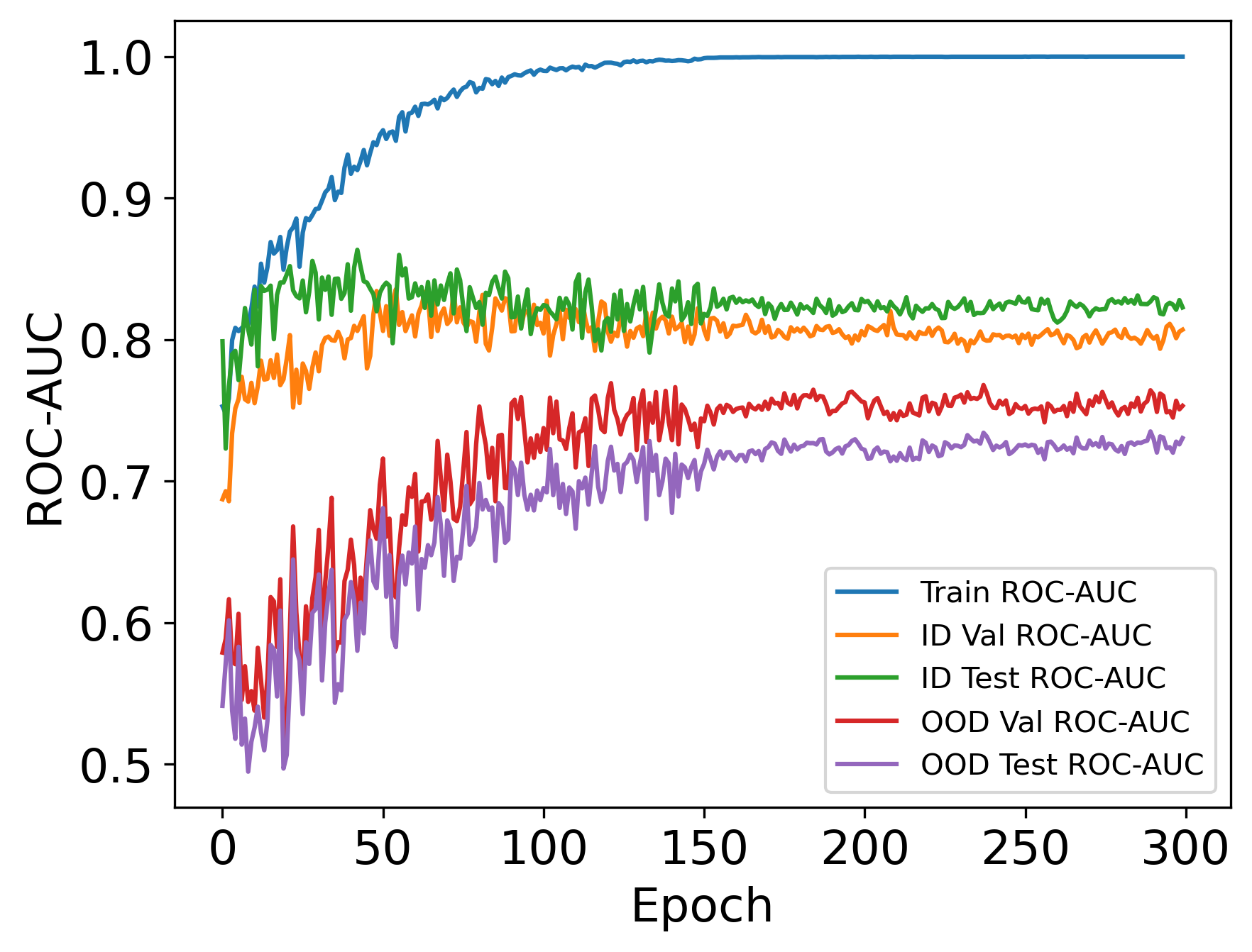
(b) concept shift + scaffold domain

(c) covariate shift + size domain

(d) concept shift + size domain

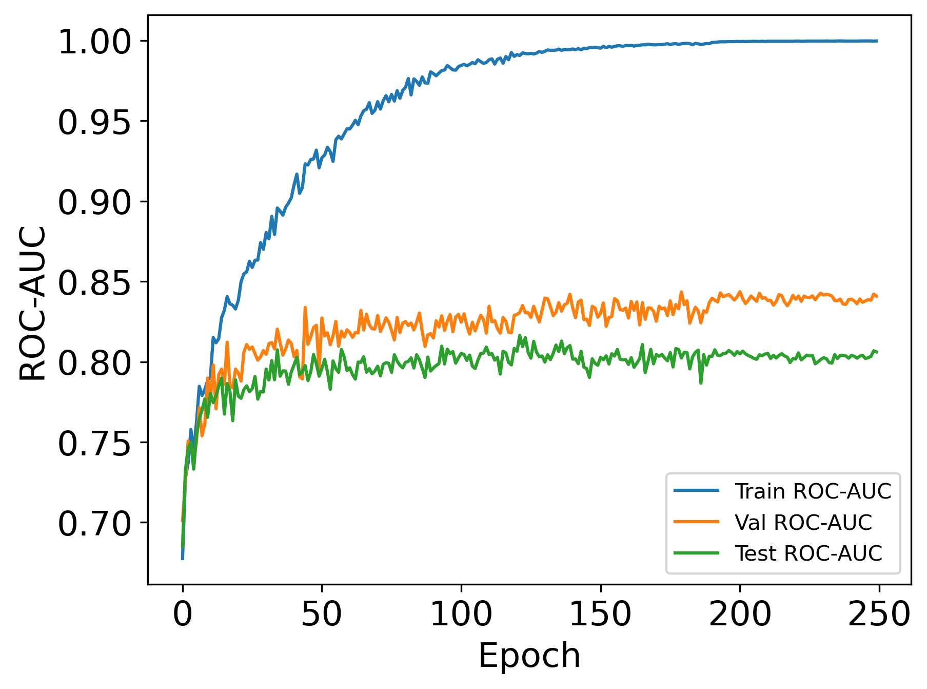
(e) no shift

Figure 3: Metric score curves for ERM on GOOD-HIV. Note that we omit the domain selection for no shift since the two cases make no difference in results.

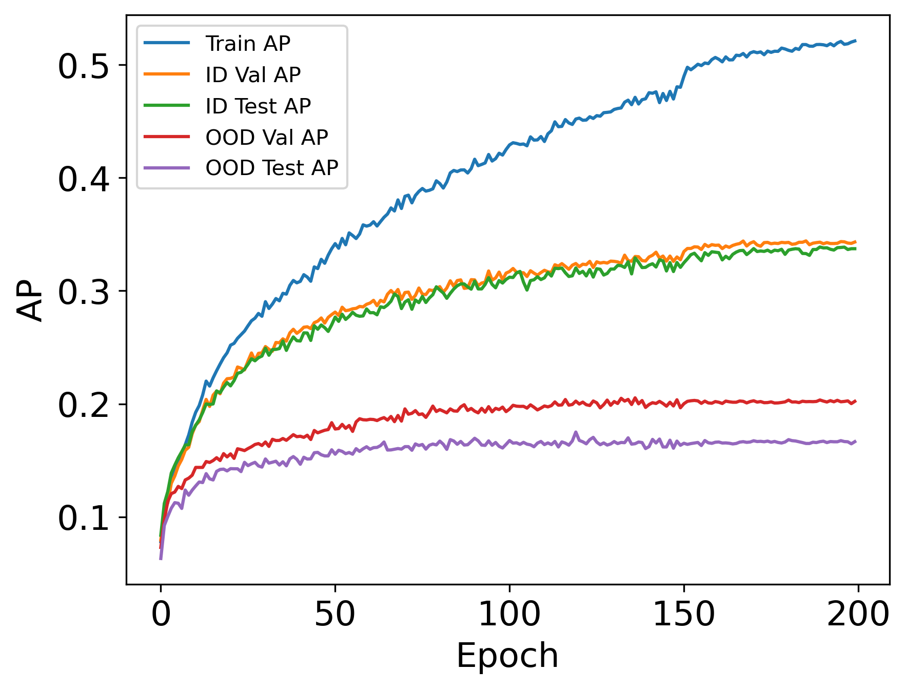
(a) scaffold domain, covariate shift

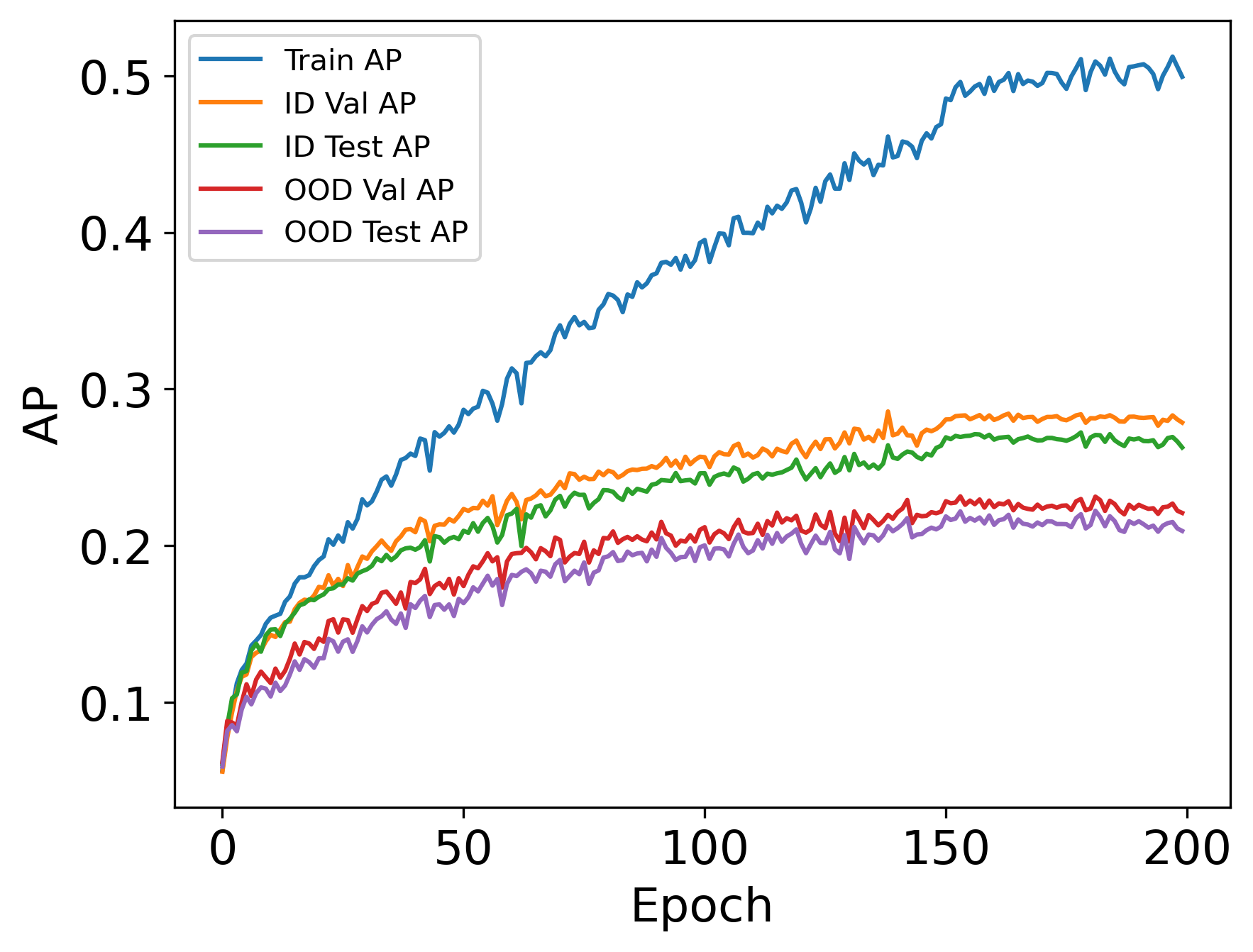
(b) concept shift + scaffold domain

(c) covariate shift + size domain

(d) concept shift + size domain

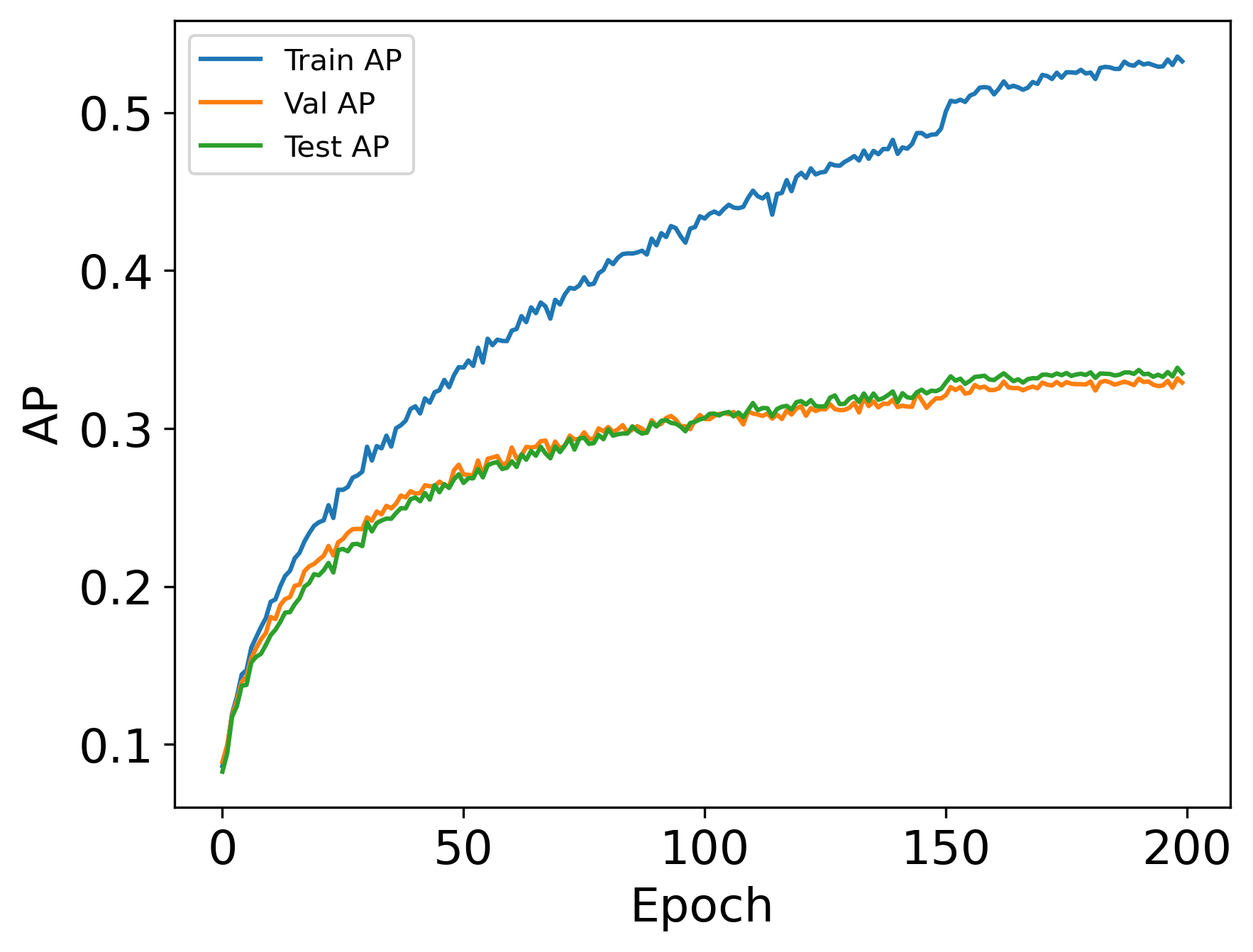
(e) no shift

Figure 4: Metric score curves for ERM on GOOD-PCBA.

(a) covariate shift + scaffold domain

(b) concept shift + scaffold domain

(c) covariate shift + size domain

(d) concept shift + size domain

(e) no shift

Figure 5: Metric score curves for ERM on GOOD-ZINC.

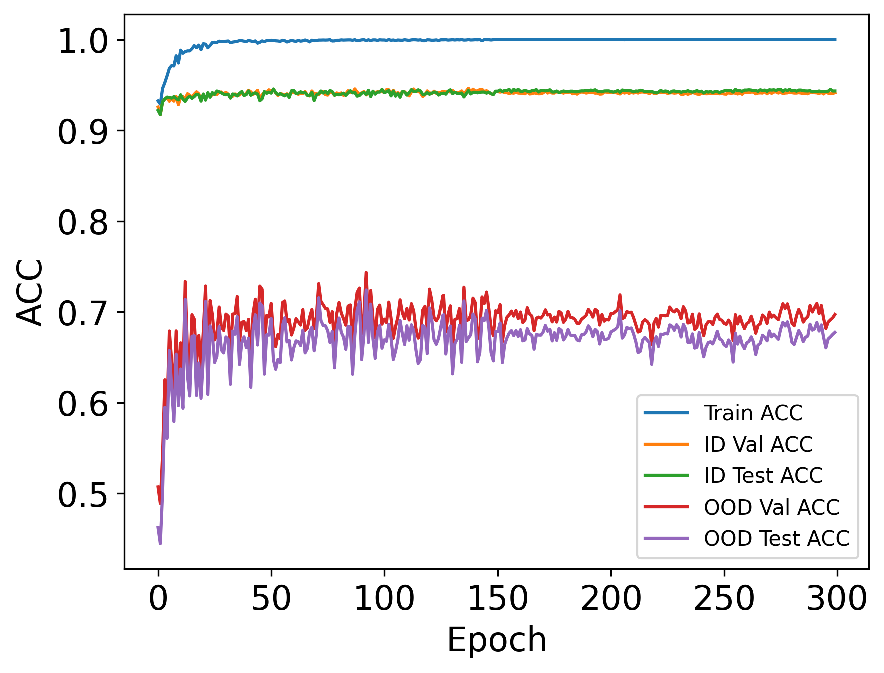
(a) concept shift + length domain

(b) covariate shift + length domain

(c) no shift + length domain

Figure 6: Metric score curves for ERM on GOOD-SST2.

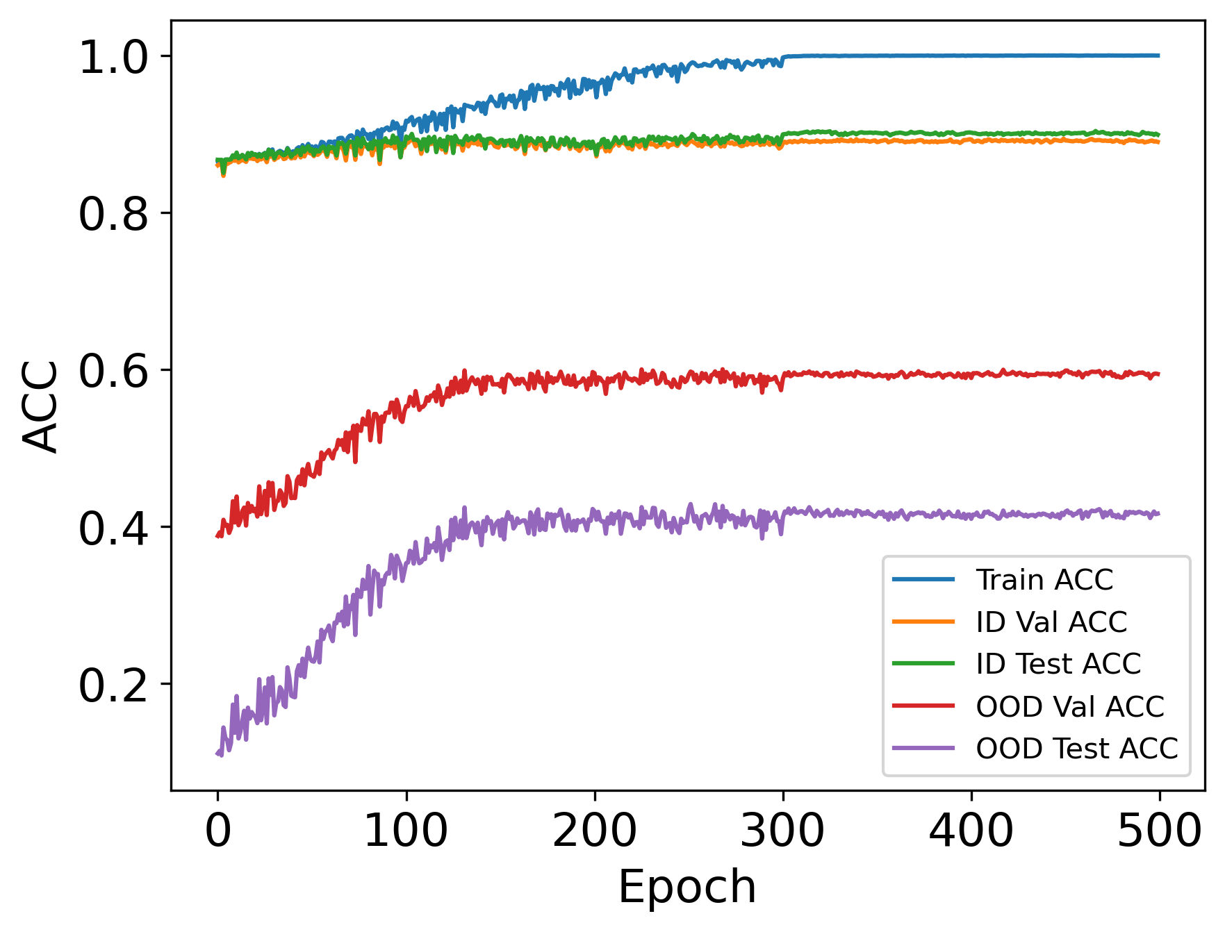
(a) concept shift + color domain

(b) covariate shift + color domain

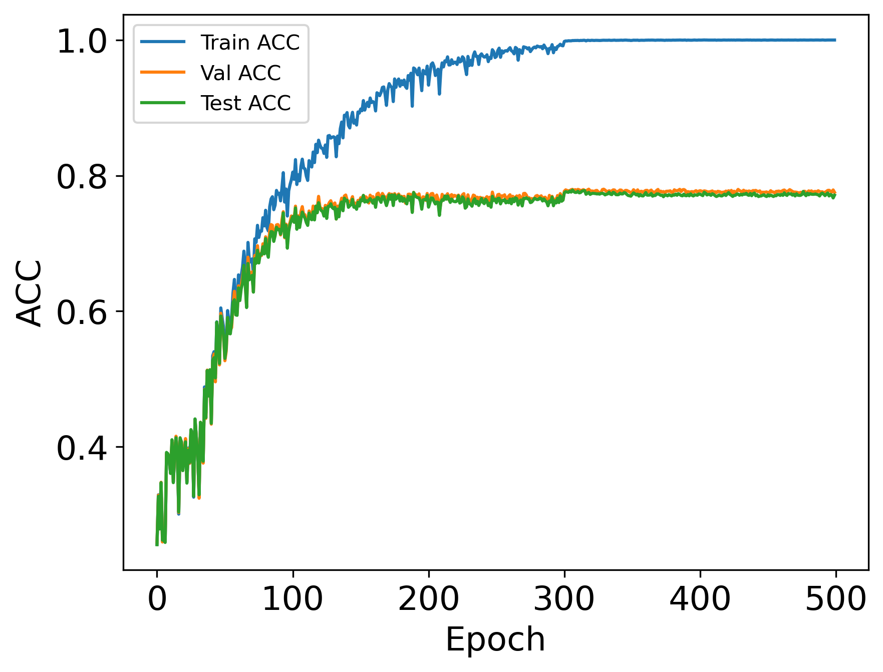
(c) no shift + color domain

Figure 7: Metric score curves for ERM on GOOD-CMNIST.

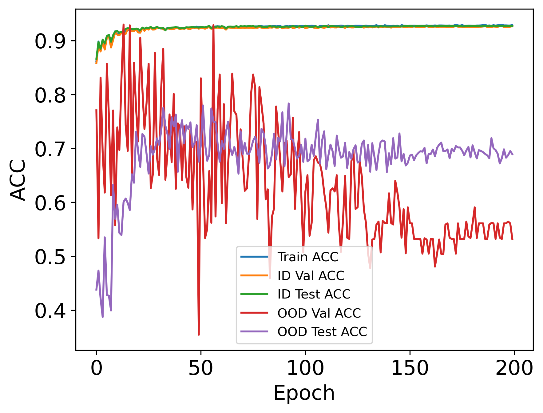
(a) covariate shift + base domain

(b) concept shift + base domain

(c) covariate shift + size domain

(d) concept shift + size domain

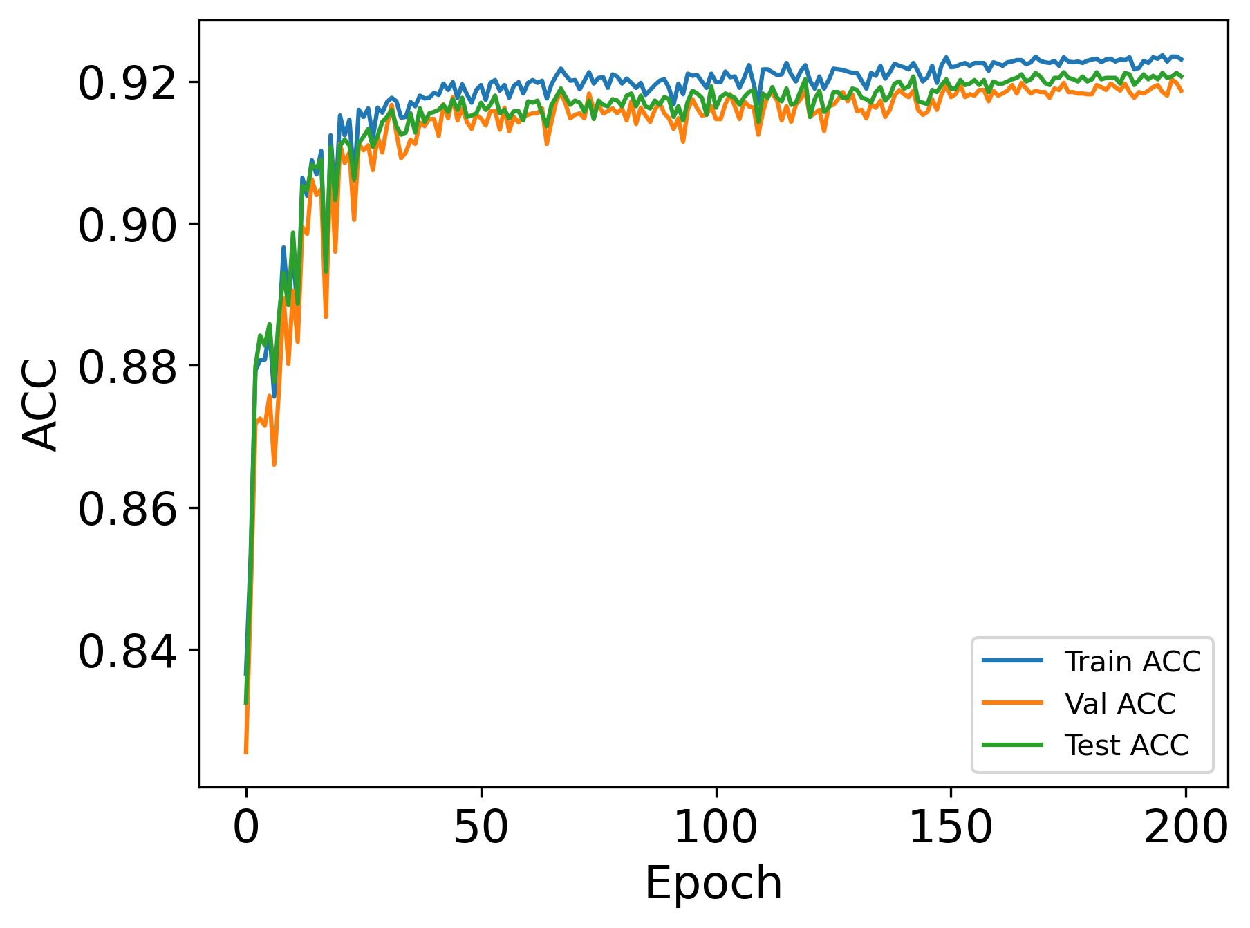
(e) no shift

Figure 8: Metric score curves for ERM on GOOD-Motif.

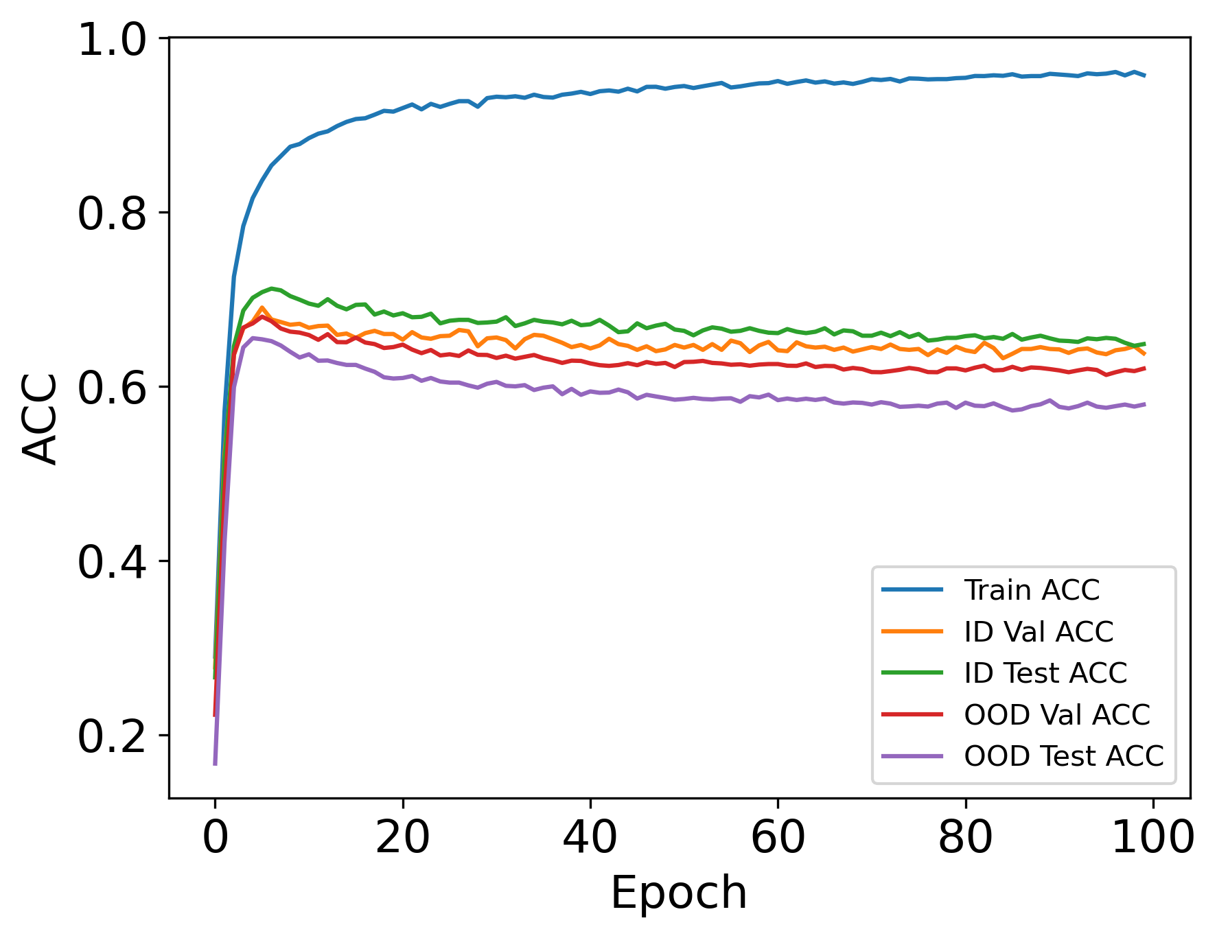
(a) covariate shift + word domain

(b) concept shift + word domain

(c) no shift + word domain

(d) covariate shift + degree domain

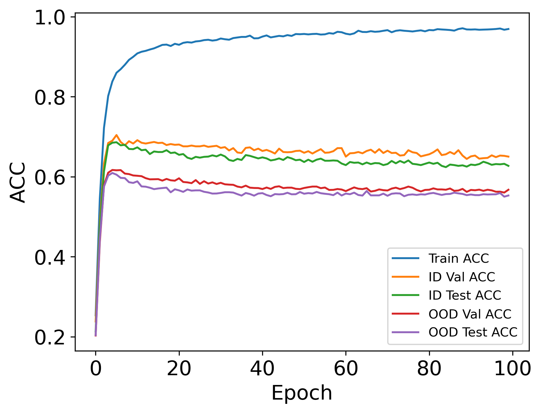
(e) concept shift + degree domain

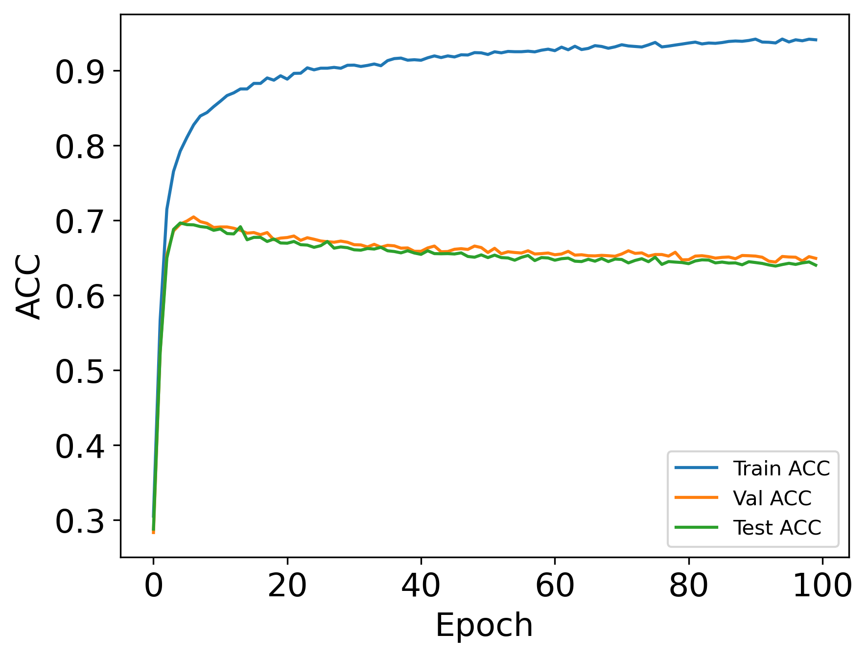
(f) no shift + degree domain

Figure 9: Metric score curves for ERM on GOOD-Cora.

(a) covariate shift + time domain

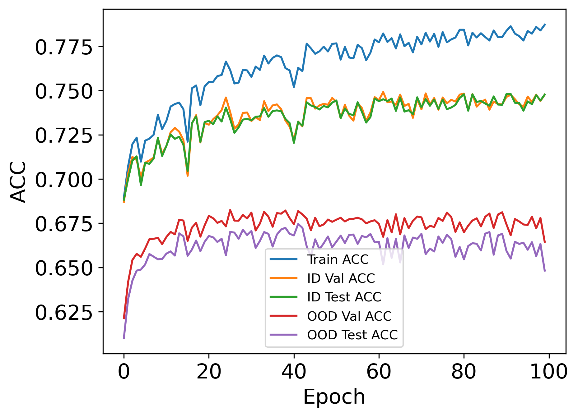
(b) concept shift + time domain

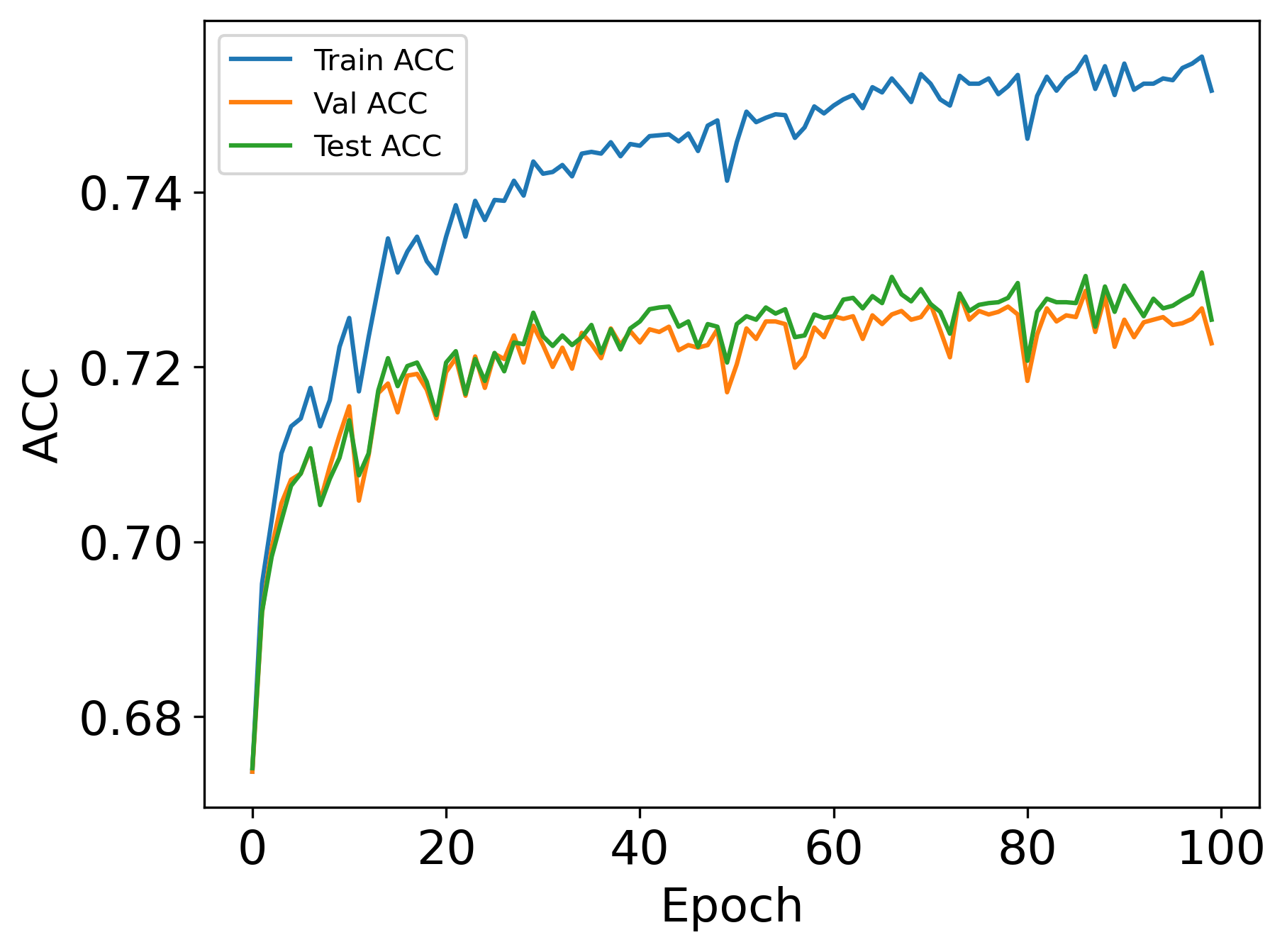
(c) no shift + time domain

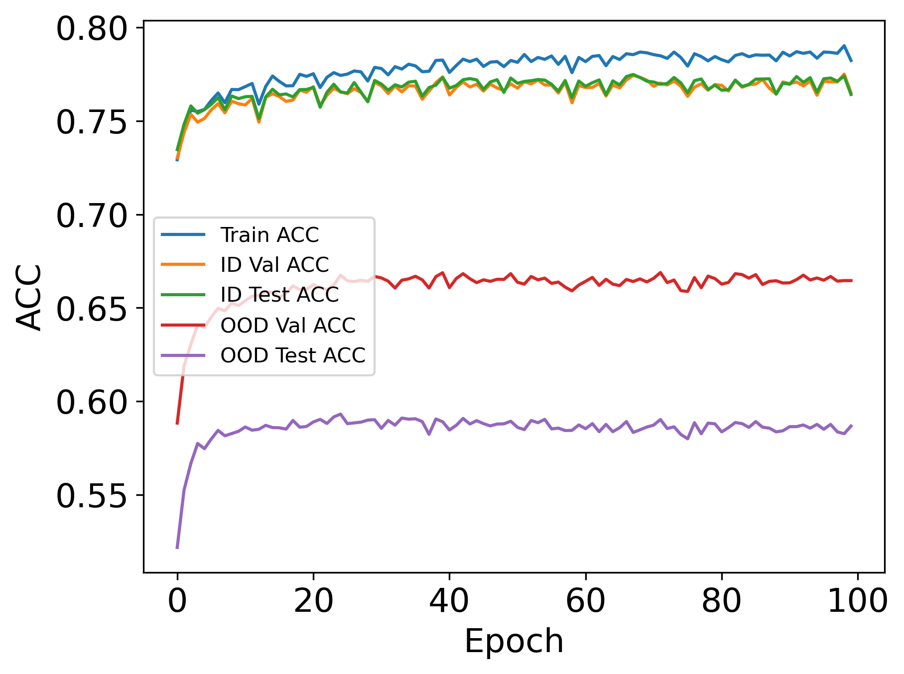
(d) covariate shift + degree domain

(e) concept shift + degree domain

(f) no shift + degree domain

Figure 10: Metric score curves for ERM on GOOD-Arxiv.

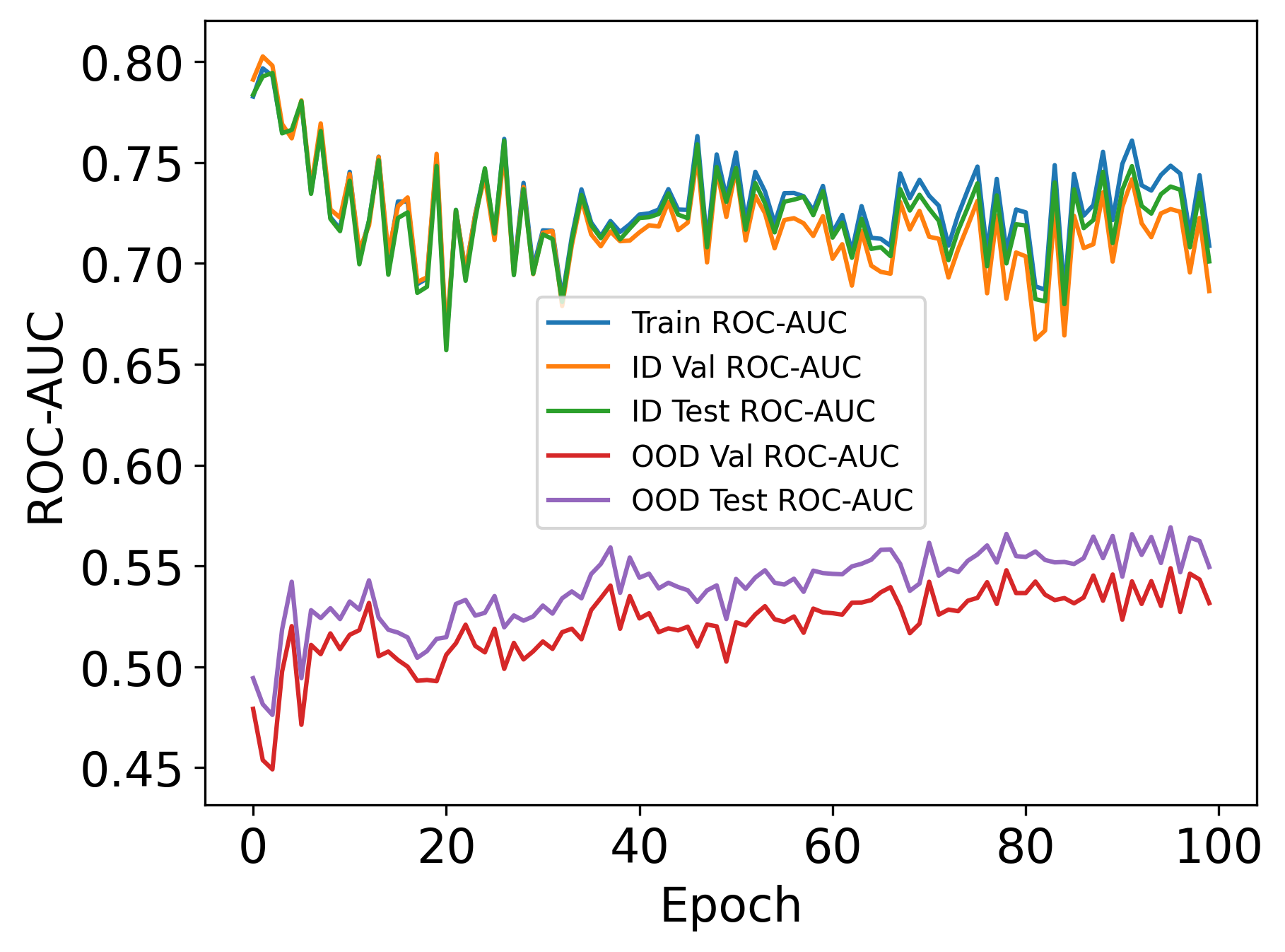
(a) covariate shift + language domain

(b) concept shift + language domain

(c) no shift + language domain

Figure 11: Metric score curves for ERM on GOOD-Twitch.

(a) covariate shift + university domain

(b) concept shift + university domain

(c) no shift + university domain

Figure 12: Metric score curves for ERM on GOOD-WebKB.

(a) covariate shift + color domain

(b) concept shift + color domain

(c) no shift + color domain

Figure 13: Metric score curves for ERM on GOOD-CBAS.

D.3 Comparison between training, validation and test scores

To directly view performance gaps between training and test data, we compare training, validation, and test scores in Table 22. These comparisons reveal the distribution shift by definition.

Dataset			Domain	Shift	ID validation				OOD validation
					Train	Validation	ID test	OOD test	Train	Validation	ID test	OOD test
GOOD-HIV↑			scaffold	covariate	99.40	84.11	82.62	68.65	91.63	78.94	81.49	69.57
				concept	94.04	83.56	82.63	58.28	99.56	76.92	80.55	72.43
			size	covariate	99.76	86.34	83.58	59.26	87.84	74.86	82.14	54.68
				concept	98.53	91.93	88.38	50.07	99.97	61.48	83.89	63.38
GOOD-PCBA↑			scaffold	covariate	51.57	33.74	32.75	17.01	47.95	20.75	32.76	16.49
				concept	47.86	28.42	25.86	20.40	49.57	22.00	26.08	21.24
			size	covariate	52.91	33.89	34.17	18.26	52.91	27.23	34.17	18.26
				concept	55.16	34.56	33.64	16.45	55.78	17.32	33.36	16.49
GOOD-ZINC↓			scaffold	covariate	0.1183	0.1224	0.1224	0.1895	0.1380	0.1421	0.1409	0.2159
				concept	0.1074	0.1138	0.1128	0.1243	0.1086	0.1232	0.1141	0.1239
			size	covariate	0.1167	0.1215	0.1214	0.2581	0.1210	0.1313	0.1259	0.2352
				concept	0.1117	0.1142	0.1162	0.1370	0.1244	0.1286	0.1298	0.1279
GOOD-SST2↑			length	covariate	100.00	90.10	89.81	76.03	99.79	85.78	88.74	80.58
				concept	100.00	94.64	94.39	67.13	99.90	74.34	93.96	72.41
GOOD-CMNIST↑			color	covariate	93.54	77.83	77.17	26.39	97.07	64.39	76.97	29.49
				concept	92.15	89.46	90.00	36.68	99.13	60.01	89.40	42.60
GOOD-Motif↑			base	covariate	92.90	92.70	92.67	70.43	91.60	90.53	91.93	66.57
				concept	93.06	92.74	91.96	80.37	93.08	84.45	92.00	80.78
			size	covariate	92.06	92.87	92.40	55.63	91.85	88.57	92.17	54.33
				concept	91.80	92.63	91.81	69.93	91.97	76.67	91.81	71.35
GOOD-Cora↑			word	covariate	83.61	69.02	70.79	65.38	83.61	67.98	70.79	65.38
				concept	84.96	71.22	65.77	64.84	84.96	65.92	65.77	64.84
			degree	covariate	82.98	72.46	72.36	56.25	81.29	64.30	72.92	56.49
				concept	85.98	70.41	68.61	60.51	83.80	61.68	68.49	60.93
GOOD-Arxiv↑			time	covariate	76.74	73.70	73.00	70.30	76.69	72.21	72.66	71.16
				concept	78.23	74.92	74.51	65.17	76.17	68.25	73.39	67.01
			degree	covariate	79.02	77.50	77.39	58.27	78.48	66.89	76.96	59.03
				concept	79.79	76.43	75.43	61.85	77.33	63.77	74.41	62.75
GOOD-Twitch↑			language	covariate	70.11	69.06	70.98	48.24	68.55	50.95	69.87	54.76
				concept	79.67	80.26	79.27	48.15	74.84	54.89	73.81	56.92
GOOD-WebKB↑			university	covariate	95.08	59.02	39.34	9.52	90.57	22.40	34.43	18.25
				concept	74.82	63.33	61.67	25.69	98.58	33.02	60.00	26.61
GOOD-CBAS↑			color	covariate	94.05	82.86	82.86	70.00	99.76	80.00	91.43	77.14
				concept	100.00	92.14	87.86	82.86	100.00	89.29	90.71	81.43

Table 22: Comparison between training, validation and test scores for ERM on 11 datasets. The scores are evaluated on the final model of a random run. ↑ indicates higher values correspond to better performance while ↓ indicates lower values for better performance.

Appendix E Complete OOD Parameter Selections

Following Appendix B, in this section we specify the hyperparameter tune set and selection for each algorithm on each dataset in Table 23-33.

GOOD-HIV			tune set			scaffold			size
						covariate	concept	no shift	covariate	concept	no shift
ERM			–	–	–	–	–	–	–	–	–
IRM			10.0	0.1	1.0	1.0	0.1	0.1	10.0	0.1	0.1
VREx			10.0	1000.0	100.0	100.0	10.0	100.0	10.0	1000.0	100.0
GroupDRO			0.01	0.1	0.001	0.1	0.01	0.001	0.01	0.001	0.001
DANN			0.1	1.0	0.01	1.0	0.1	0.01	0.01	1.0	0.01
Deep Coral			0.01	1.0	0.1	0.1	0.01	0.01	0.1	0.01	0.01
Mixup			1.0	2.0	0.4	2.0	0.4	2.0	2.0	0.4	2.0
DIR			0.4	0.6	0.8	0.8	0.8	0.8	0.8	0.8	0.8

Table 23: OOD hyperparameter selections on GOOD-HIV.

GOOD-PCBA			tune set			scaffold			size
						covariate	concept	no shift	covariate	concept	no shift
ERM			–	–	–	–	–	–	–	–	–
IRM			1.0	0.1	10.0	0.1	0.1	0.1	0.1	1.0	0.1
VREx			10.0	100.0	1.0	10.0	100.0	10.0	1.0	10.0	10.0
GroupDRO			0.01	0.001	0.1	0.01	0.001	0.1	0.1	0.01	0.1
DANN			0.01	0.001	0.1	0.01	0.01	0.01	0.01	0.01	0.01
Deep Coral			0.1	0.01	1.0	0.01	0.1	1.0	0.1	0.1	1.0
Mixup			1.0	2.0	0.4	1.0	2.0	1.0	2.0	1.0	1.0
DIR			0.4	0.6	0.8	0.8	0.8	0.8	0.8	0.8	0.8

Table 24: OOD hyperparameter selections on GOOD-PCBA.

GOOD-ZINC			tune set			scaffold			size
						covariate	concept	no shift	covariate	concept	no shift
ERM			–	–	–	–	–	–	–	–	–
IRM			1.0	0.1	0.01	0.01	0.01	0.01	0.01	0.01	0.01
VREx			100.0	10.0	1000.0	1000.0	100.0	100.0	1000.0	100.0	100.0
GroupDRO			0.01	0.1	0.001	0.1	0.001	0.1	0.001	0.001	0.1
DANN			0.01	0.001	0.1	0.001	0.001	0.1	0.01	0.1	0.1
Deep Coral			0.1	0.01	1.0	1.0	1.0	1.0	1.0	1.0	1.0
Mixup			1.0	0.4	2.0	0.4	1.0	1.0	1.0	0.4	1.0
DIR			0.4	0.6	0.8	0.8	0.8	0.8	0.8	0.8	0.8

Table 25: OOD hyperparameter selections on GOOD-ZINC.

GOOD-SST2			tune set			length
						covariate	concept	no shift
ERM			–	–	–	–	–	–
IRM			0.1	1.0	10.0	0.1	10.0	1.0
VREx			1000.0	100.0	10.0	100.0	100.0	10.0
GroupDRO			0.01	0.001	0.1	0.01	0.001	0.001
DANN			0.1	0.01	1.0	0.01	0.1	0.01
Deep Coral			0.1	1.0	0.01	1.0	1.0	0.1
Mixup			0.4	2.0	1.0	1.0	1.0	1.0
DIR			0.6	0.7	0.8	0.8	0.7	0.8

Table 26: OOD hyperparameter selections on GOOD-SST2.

GOOD-CMNIST			tune set			color
						covariate	concept	no shift
ERM			–	–	–	–	–	–
IRM			0.1	1.0	0.01	0.1	0.1	1.0
VREx			0.01	0.1	1.0	1.0	0.01	0.1
GroupDRO			0.001	0.01	0.1	0.1	0.01	0.1
DANN			0.1	0.01	0.001	0.1	0.01	0.001
Deep Coral			0.1	0.01	0.001	0.1	0.0001	0.001
Mixup			1.0	2.0	0.4	1.0	0.4	0.4
DIR			0.4	0.6	0.8	0.6	0.6	0.6

Table 27: OOD hyperparameter selections on GOOD-CMNIST.

GOOD-Motif			tune set			base			size
						covariate	concept	no shift	covariate	concept	no shift
ERM			–	–	–	–	–	–	–	–	–
IRM			1.0	10.0	0.1	0.1	0.1	0.1	0.1	0.1	0.1
VREx			1000.0	100.0	10.0	1000.0	1000.0	1000.0	100.0	10.0	1000.0
GroupDRO			0.001	0.01	0.1	0.001	0.001	0.1	0.1	0.01	0.1
DANN			0.1	1.0	0.01	0.01	0.1	0.01	0.1	0.1	0.01
Deep Coral			1.0	0.1	0.01	1.0	0.1	0.1	1.0	0.01	0.1
Mixup			1.0	2.0	0.4	2.0	0.4	0.4	1.0	0.4	0.4
DIR			0.2	0.25	0.3	0.25	0.3	0.25	0.25	0.3	0.25

Table 28: OOD hyperparameter selections on GOOD-Motif.

GOOD-Cora			tune set			word			degree
						covariate	concept	no shift	covariate	concept	no shift
ERM			–	–	–	–	–	–	–	–	–
IRM			0.1	1.0	10.0	10.0	0.1	0.1	1.0	10.0	0.1
VREx			100.0	10.0	1.0	100.0	10.0	1.0	10.0	10.0	1.0
GroupDRO			0.001	0.01	0.1	0.1	0.01	0.01	0.1	0.01	0.01
DANN			0.01	0.1	0.001	0.001	0.1	0.001	0.01	0.1	0.001
Deep Coral			0.01	0.1	1.0	0.01	0.01	1.0	1.0	0.1	0.01
Mixup			0.4	2.0	1.0	0.4	2.0	0.4	0.4	2.0	2.0
EERM			1/3, 1e-2/5e-3/1e-2/1e-4			1,5e-3	3,1e-3	3,1e-2	3,5e-3	3,1e-3	3,1e-2
SRGNN			1e-5	1e-6	1e-4	1e-4	1e-5	1e-6	1e-5	1e-6	1e-6

Table 29: OOD hyperparameter selections on GOOD-Cora.

GOOD-Arxiv			tune set			time			degree
						covariate	concept	no shift	covariate	concept	no shift
ERM			–	–	–	–	–	–	–	–	–
IRM			0.1	1.0	10.0	0.1	1.0	1.0	0.1	1.0	1.0
VREx			1.0	100.0	10.0	100.0	1.0	100.0	1.0	100.0	1.0
GroupDRO			0.001	0.01	0.1	0.01	0.001	0.1	0.1	0.001	0.1
DANN			0.1	0.001	0.01	0.001	0.001	0.001	0.01	0.001	0.1
Deep Coral			0.1	0.01	1.0	0.1	1.0	1.0	0.1	1.0	0.1
Mixup			2.0	1.0	0.4	1.0	0.4	0.4	2.0	1.0	1.0
EERM			–	–	–	–	–	–	–	–	–
SRGNN			1e-5	1e-6	1e-4	1e-6	1e-6	1e-6	1e-6	1e-5	1e-6

Table 30: OOD hyperparameter selections on GOOD-Arxiv.

GOOD-Twitch			tune set			language
						covariate	concept	no shift
ERM			–	–	–	–	–	–
IRM			10.0	0.1	1.0	10.0	1.0	0.1
VREx			100.0	10.0	1.0	100.0	100.0	10.0
GroupDRO			0.001	0.1	0.01	0.1	0.1	0.001
DANN			0.1	0.01	0.001	0.01	0.001	0.01
Deep Coral			0.01	1.0	0.1	0.01	0.01	0.1
Mixup			2.0	0.4	1.0	0.4	0.4	0.4
EERM			1/3, 1e-2/5e-3/1e-2/1e-4			1,1e-2	3,5e-3	3,1e-2
SRGNN			1e-5	1e-6	1e-4	1e-5	1e-6	1e-6

Table 31: OOD hyperparameter selections on GOOD-Twitch.

GOOD-WebKB			tune set			university
						covariate	concept	no shift
ERM			–	–	–	–	–	–
IRM			10.0	1.0	0.1	10.0	10.0	10.0
VREx			10.0	100.0	1.0	10.0	10.0	1.0
GroupDRO			0.01	0.001	0.1	0.001	0.01	0.1
DANN			0.001	0.01	0.1	0.001	0.01	0.001
Deep Coral			0.1	1.0	0.01	0.01	0.01	1.0
Mixup			0.4	1.0	2.0	2.0	0.4	2.0
EERM			1/3, 1e-2/5e-3/1e-2/1e-4			3,1e-3	3,5e-3	3,1e-3
SRGNN			1e-5	1e-6	1e-4	1e-6	1e-5	1e-4

Table 32: OOD hyperparameter selections on GOOD-WebKB.

GOOD-CBAS			tune set			color
						covariate	concept	no shift
ERM			–	–	–	–	–	–
IRM			10.0	1.0	0.1	10.0	1.0	10.0
VREx			100.0	1.0	10.0	100.0	100.0	1.0
GroupDRO			0.1	0.01	0.001	0.1	0.001	0.01
DANN			0.01	0.001	0.1	0.1	0.1	0.01
Deep Coral			0.01	0.1	0.001	0.01	0.001	0.01
Mixup			0.4	1.0	2.0	0.4	2.0	0.4
EERM			1/3, 1e-2/5e-3/1e-2/1e-4			1,5e-3	1,1e-2	1,1e-2
SRGNN			1e-5	1e-6	1e-4	1e-5	1e-5	1e-6

Table 33: OOD hyperparameter selections on GOOD-CBAS.

Appendix F GOOD Usage Guidelines and Maintenance Schedule

We provide the open-source GOOD project to reproduce all reported results and extend OOD datasets and algorithms. The GOOD project enables automatic dataset downloads, easy data loading, and handy start-up code to work with any GOOD dataset or method. Meanwhile, we provide various modular utilities for OOD method development. Reproduction is available and effortless with given test scripts and automatic re-loading of our best checkpoints. Please refer to our GitHub repository for installation details, along with more documentation and usage information at https://github.com/divelab/GOOD/. The code of GOOD uses the GPL3.0 license, while the datasets follow the MIT license. Please refer to the GOOD GitHub repository for license details.

We provide simple and standardized examples for dataset loading and training/evaluation procedures.

F.1 GOOD dataset loading

Code listing 14 shows two ways to import a GOOD dataset and specify the domain selection and shift split.

F.2 GOOD taining/test pipeline

Code listing 15 provides a script to use the main function of the training/evaluation pipeline, following the three steps of loading the config, specifying the model, and executing the task.

F.3 Maintenance schedule

GOOD is maintained on GitHub, with CI tests hosted by CircleCI. We welcome public use of the community. Any issues or discussions regarding technical or other concerns can be submitted to the GitHub repository, and we will reply as soon as possible. GOOD benchmark is a growing project and expects to include more datasets, splits, and methods along with the development of the field. We expect to include more methods in future work, especially graph-related ones. We will also include datasets and domain selections of a larger quantity and variety. In addition, the current benchmark does not consider link prediction tasks [59], which will be added as the project develops.

GOOD provides simple APIs for loading OOD algorithms, graph neural networks, and datasets, taking only several lines of code to start. The full OOD split generalization code is provided for extensions and any new graph OOD dataset contributions. OOD algorithm base class can be easily overwritten to create new OOD methods. In addition to playing as a package, GOOD is also an integrated and well-organized project ready to be further developed. All algorithms, models, and datasets can be easily registered by the register and automatically embedded into the designed pipeline without much effort. The only thing the user needs to do is write their own OOD algorithm class, model class, or new dataset class. Then they can compare their results with the leaderboard. We provide insightful comparisons from multiple perspectives. Any research and studies can use our leaderboard results for comparison. Note that this is a growing project, so we will include new OOD algorithms gradually. Besides, we welcome researchers to include their algorithms in the leaderboard. We welcome and will assist with any contributions to this project. We expect GOOD as a graph OOD research, study, and development toolkit of easy use.

Figure 14: GOOD dataset loader

Figure 15: GOOD taining/test pipeline

References

- Ahuja et al. [2021] Kartik Ahuja, Ethan Caballero, Dinghuai Zhang, Jean-Christophe Gagnon-Audet, Yoshua Bengio, Ioannis Mitliagkas, and Irina Rish. Invariance principle meets information bottleneck for out-of-distribution generalization. Advances in Neural Information Processing Systems, 34:3438–3450, 2021.
- Alaiz-Rodríguez and Japkowicz [2008] Rocío Alaiz-Rodríguez and Nathalie Japkowicz. Assessing the impact of changing environments on classifier performance. In Conference of the Canadian Society for Computational Studies of Intelligence, pages 13–24. Springer, 2008.
- Arjovsky et al. [2019] Martin Arjovsky, Léon Bottou, Ishaan Gulrajani, and David Lopez-Paz. Invariant risk minimization. arXiv preprint arXiv:1907.02893, 2019.
- Bemis and Murcko [1996] Guy W Bemis and Mark A Murcko. The properties of known drugs. 1. molecular frameworks. Journal of medicinal chemistry, 39(15):2887–2893, 1996.
- Ben-David et al. [2010] Shai Ben-David, John Blitzer, Koby Crammer, Alex Kulesza, Fernando Pereira, and Jennifer Wortman Vaughan. A theory of learning from different domains. Machine learning, 79(1):151–175, 2010.
- Bevilacqua et al. [2021] Beatrice Bevilacqua, Yangze Zhou, and Bruno Ribeiro. Size-invariant graph representations for graph classification extrapolations. In International Conference on Machine Learning, pages 837–851. PMLR, 2021.
- Bojchevski and Günnemann [2017] Aleksandar Bojchevski and Stephan Günnemann. Deep gaussian embedding of graphs: Unsupervised inductive learning via ranking. arXiv preprint arXiv:1707.03815, 2017.
- Chen et al. [2022] Yongqiang Chen, Yonggang Zhang, Han Yang, Kaili Ma, Binghui Xie, Tongliang Liu, Bo Han, and James Cheng. Invariance principle meets out-of-distribution generalization on graphs. arXiv preprint arXiv:2202.05441, 2022.
- Ding et al. [2021] Mucong Ding, Kezhi Kong, Jiuhai Chen, John Kirchenbauer, Micah Goldblum, David Wipf, Furong Huang, and Tom Goldstein. A closer look at distribution shifts and out-of-distribution generalization on graphs. In NeurIPS 2021 Workshop on Distribution Shifts: Connecting Methods and Applications, 2021. URL https://openreview.net/forum?id=XvgPGWazqRH.
- Fan et al. [2021] Shaohua Fan, Xiao Wang, Chuan Shi, Peng Cui, and Bai Wang. Generalizing graph neural networks on out-of-distribution graphs. arXiv preprint arXiv:2111.10657, 2021.
- Fey and Lenssen [2019] Matthias Fey and Jan Eric Lenssen. Fast graph representation learning with PyTorch Geometric. arXiv preprint arXiv:1903.02428, 2019.
- Ganin et al. [2016] Yaroslav Ganin, Evgeniya Ustinova, Hana Ajakan, Pascal Germain, Hugo Larochelle, François Laviolette, Mario Marchand, and Victor Lempitsky. Domain-adversarial training of neural networks. The journal of machine learning research, 17(1):2096–2030, 2016.
- Gao and Ji [2019] Hongyang Gao and Shuiwang Ji. Graph U-nets. In international conference on machine learning, pages 2083–2092. PMLR, 2019.
- Gao et al. [2021] Hongyang Gao, Yi Liu, and Shuiwang Ji. Topology-aware graph pooling networks. IEEE Transactions on Pattern Analysis and Machine Intelligence, 43(12):4512–4518, 2021.
- Gilmer et al. [2017] Justin Gilmer, Samuel S Schoenholz, Patrick F Riley, Oriol Vinyals, and George E Dahl. Neural message passing for quantum chemistry. In International conference on machine learning, pages 1263–1272. PMLR, 2017.
- Gómez-Bombarelli et al. [2018] Rafael Gómez-Bombarelli, Jennifer N Wei, David Duvenaud, José Miguel Hernández-Lobato, Benjamín Sánchez-Lengeling, Dennis Sheberla, Jorge Aguilera-Iparraguirre, Timothy D Hirzel, Ryan P Adams, and Alán Aspuru-Guzik. Automatic chemical design using a data-driven continuous representation of molecules. ACS central science, 4(2):268–276, 2018.
- Gulrajani and Lopez-Paz [2020] Ishaan Gulrajani and David Lopez-Paz. In search of lost domain generalization. arXiv preprint arXiv:2007.01434, 2020.
- Hand [2006] David J Hand. Classifier technology and the illusion of progress. Statistical science, 21(1):1–14, 2006.
- He et al. [2021] Yue He, Zheyan Shen, and Peng Cui. Towards non-iid image classification: A dataset and baselines. Pattern Recognition, 110:107383, 2021.
- Hu et al. [2020] Weihua Hu, Matthias Fey, Marinka Zitnik, Yuxiao Dong, Hongyu Ren, Bowen Liu, Michele Catasta, and Jure Leskovec. Open graph benchmark: Datasets for machine learning on graphs. Advances in neural information processing systems, 33:22118–22133, 2020.
- Ji et al. [2022] Yuanfeng Ji, Lu Zhang, Jiaxiang Wu, Bingzhe Wu, Long-Kai Huang, Tingyang Xu, Yu Rong, Lanqing Li, Jie Ren, Ding Xue, et al. DrugOOD: Out-of-distribution (OOD) dataset curator and benchmark for AI-aided drug discovery–a focus on affinity prediction problems with noise annotations. arXiv preprint arXiv:2201.09637, 2022.
- Jin et al. [2018] Wengong Jin, Regina Barzilay, and Tommi Jaakkola. Junction tree variational autoencoder for molecular graph generation. In International conference on machine learning, pages 2323–2332. PMLR, 2018.
- Kipf and Welling [2017] Thomas N. Kipf and Max Welling. Semi-supervised classification with graph convolutional networks. In International Conference on Learning Representations (ICLR), 2017.
- Koh et al. [2021] Pang Wei Koh, Shiori Sagawa, Henrik Marklund, Sang Michael Xie, Marvin Zhang, Akshay Balsubramani, Weihua Hu, Michihiro Yasunaga, Richard Lanas Phillips, Irena Gao, et al. Wilds: A benchmark of in-the-wild distribution shifts. In International Conference on Machine Learning, pages 5637–5664. PMLR, 2021.
- Krueger et al. [2021] David Krueger, Ethan Caballero, Joern-Henrik Jacobsen, Amy Zhang, Jonathan Binas, Dinghuai Zhang, Remi Le Priol, and Aaron Courville. Out-of-distribution generalization via risk extrapolation (REx). In International Conference on Machine Learning, pages 5815–5826. PMLR, 2021.
- Kusner et al. [2017] Matt J Kusner, Brooks Paige, and José Miguel Hernández-Lobato. Grammar variational autoencoder. In International conference on machine learning, pages 1945–1954. PMLR, 2017.
- Li et al. [2021] Haoyang Li, Xin Wang, Ziwei Zhang, and Wenwu Zhu. OOD-GNN: Out-of-distribution generalized graph neural network. arXiv preprint arXiv:2112.03806, 2021.
- Li et al. [2022] Haoyang Li, Xin Wang, Ziwei Zhang, and Wenwu Zhu. Out-of-distribution generalization on graphs: A survey. arXiv preprint arXiv:2202.07987, 2022.
- Liu et al. [2021] Meng Liu, Youzhi Luo, Limei Wang, Yaochen Xie, Hao Yuan, Shurui Gui, Haiyang Yu, Zhao Xu, Jingtun Zhang, Yi Liu, et al. DIG: a turnkey library for diving into graph deep learning research. Journal of Machine Learning Research, 22(240):1–9, 2021.
- Liu et al. [2022a] Meng Liu, Haiyang Yu, and Shuiwang Ji. Your neighbors are communicating: Towards powerful and scalable graph neural networks. https://arxiv.org/abs/2206.02059, 2022a.
- Liu et al. [2020] Yi Liu, Hao Yuan, Lei Cai, and Shuiwang Ji. Deep learning of high-order interactions for protein interface prediction. In Proceedings of the 26th ACM SIGKDD international conference on knowledge discovery & data mining, pages 679–687, 2020.
- Liu et al. [2022b] Yi Liu, Limei Wang, Meng Liu, Yuchao Lin, Xuan Zhang, Bora Oztekin, and Shuiwang Ji. Spherical message passing for 3d molecular graphs. In International Conference on Learning Representations, 2022b. URL https://openreview.net/forum?id=givsRXsOt9r.
- Lu et al. [2021] Chaochao Lu, Yuhuai Wu, José Miguel Hernández-Lobato, and Bernhard Schölkopf. Invariant causal representation learning for out-of-distribution generalization. In International Conference on Learning Representations, 2021.
- Mendez et al. [2019] David Mendez, Anna Gaulton, A Patrícia Bento, Jon Chambers, Marleen De Veij, Eloy Félix, María Paula Magariños, Juan F Mosquera, Prudence Mutowo, Michał Nowotka, et al. ChEMBL: towards direct deposition of bioassay data. Nucleic acids research, 47(D1):D930–D940, 2019.
- Monti et al. [2017] Federico Monti, Davide Boscaini, Jonathan Masci, Emanuele Rodola, Jan Svoboda, and Michael M Bronstein. Geometric deep learning on graphs and manifolds using mixture model CNNs. In Proceedings of the IEEE conference on computer vision and pattern recognition, pages 5115–5124, 2017.
- Moreno-Torres et al. [2012] Jose G Moreno-Torres, Troy Raeder, Rocío Alaiz-Rodríguez, Nitesh V Chawla, and Francisco Herrera. A unifying view on dataset shift in classification. Pattern Recognition, 45(1):521–530, 2012. ISSN 0031-3203. doi: https://doi.org/10.1016/j.patcog.2011.06.019. URL https://www.sciencedirect.com/science/article/pii/S0031320311002901.
- Pearl [2009] Judea Pearl. Causality. Cambridge university press, 2009.
- Peters et al. [2016] Jonas Peters, Peter Bühlmann, and Nicolai Meinshausen. Causal inference by using invariant prediction: identification and confidence intervals. Journal of the Royal Statistical Society: Series B (Statistical Methodology), 78(5):947–1012, 2016.
- Quiñonero-Candela et al. [2008] Joaquin Quiñonero-Candela, Masashi Sugiyama, Anton Schwaighofer, and Neil D Lawrence. Dataset shift in machine learning. Mit Press, 2008.
- Rosenfeld et al. [2020] Elan Rosenfeld, Pradeep Ravikumar, and Andrej Risteski. The risks of invariant risk minimization. arXiv preprint arXiv:2010.05761, 2020.
- Sagawa et al. [2019] Shiori Sagawa, Pang Wei Koh, Tatsunori B Hashimoto, and Percy Liang. Distributionally robust neural networks for group shifts: On the importance of regularization for worst-case generalization. arXiv preprint arXiv:1911.08731, 2019.
- Shen et al. [2021] Zheyan Shen, Jiashuo Liu, Yue He, Xingxuan Zhang, Renzhe Xu, Han Yu, and Peng Cui. Towards out-of-distribution generalization: A survey. arXiv preprint arXiv:2108.13624, 2021.
- Shimodaira [2000] Hidetoshi Shimodaira. Improving predictive inference under covariate shift by weighting the log-likelihood function. Journal of statistical planning and inference, 90(2):227–244, 2000.
- Sun and Saenko [2016] Baochen Sun and Kate Saenko. Deep coral: Correlation alignment for deep domain adaptation. In European conference on computer vision, pages 443–450. Springer, 2016.
- Tzeng et al. [2017] Eric Tzeng, Judy Hoffman, Kate Saenko, and Trevor Darrell. Adversarial discriminative domain adaptation. In Proceedings of the IEEE conference on computer vision and pattern recognition, pages 7167–7176, 2017.
- Veličković et al. [2018] Petar Veličković, Guillem Cucurull, Arantxa Casanova, Adriana Romero, Pietro Liò, and Yoshua Bengio. Graph Attention Networks. International Conference on Learning Representations, 2018. URL https://openreview.net/forum?id=rJXMpikCZ. accepted as poster.
- Wang et al. [2021] Yiwei Wang, Wei Wang, Yuxuan Liang, Yujun Cai, and Bryan Hooi. Mixup for node and graph classification. In Proceedings of the Web Conference 2021, pages 3663–3674, 2021.
- Widmer and Kubat [1996] Gerhard Widmer and Miroslav Kubat. Learning in the presence of concept drift and hidden contexts. Machine learning, 23(1):69–101, 1996.
- Wu et al. [2022a] Qitian Wu, Hengrui Zhang, Junchi Yan, and David Wipf. Handling distribution shifts on graphs: An invariance perspective. arXiv preprint arXiv:2202.02466, 2022a.
- Wu et al. [2022b] Ying-Xin Wu, Xiang Wang, An Zhang, Xiangnan He, and Tat seng Chua. Discovering invariant rationales for graph neural networks. In ICLR, 2022b.
- Wu et al. [2018] Zhenqin Wu, Bharath Ramsundar, Evan N Feinberg, Joseph Gomes, Caleb Geniesse, Aneesh S Pappu, Karl Leswing, and Vijay Pande. MoleculeNet: a benchmark for molecular machine learning. Chemical science, 9(2):513–530, 2018.
- Xu et al. [2019] Keyulu Xu, Weihua Hu, Jure Leskovec, and Stefanie Jegelka. How powerful are graph neural networks? In International Conference on Learning Representations, 2019. URL https://openreview.net/forum?id=ryGs6iA5Km.
- Ye et al. [2021] Nanyang Ye, Kaican Li, Lanqing Hong, Haoyue Bai, Yiting Chen, Fengwei Zhou, and Zhenguo Li. OoD-Bench: Benchmarking and understanding out-of-distribution generalization datasets and algorithms. arXiv preprint arXiv:2106.03721, 2021.
- Ying et al. [2019] Zhitao Ying, Dylan Bourgeois, Jiaxuan You, Marinka Zitnik, and Jure Leskovec. GNNExplainer: Generating explanations for graph neural networks. Advances in neural information processing systems, 32, 2019.
- Yuan et al. [2020] Hao Yuan, Haiyang Yu, Shurui Gui, and Shuiwang Ji. Explainability in graph neural networks: A taxonomic survey. arXiv preprint arXiv:2012.15445, 2020.
- Zeng et al. [2020] Hanqing Zeng, Hongkuan Zhou, Ajitesh Srivastava, Rajgopal Kannan, and Viktor Prasanna. GraphSAINT: Graph sampling based inductive learning method. In International Conference on Learning Representations, 2020. URL https://openreview.net/forum?id=BJe8pkHFwS.
- Zhang et al. [2017] Hongyi Zhang, Moustapha Cisse, Yann N Dauphin, and David Lopez-Paz. mixup: Beyond empirical risk minimization. arXiv preprint arXiv:1710.09412, 2017.
- Zhang et al. [2022] Xingxuan Zhang, Linjun Zhou, Renzhe Xu, Peng Cui, Zheyan Shen, and Haoxin Liu. NICO++: Towards better benchmarking for domain generalization. arXiv preprint arXiv:2204.08040, 2022.
- Zhou et al. [2022] Yangze Zhou, Gitta Kutyniok, and Bruno Ribeiro. OOD link prediction generalization capabilities of message-passing GNNs in larger test graphs. arXiv preprint arXiv:2205.15117, 2022.
- Zhu et al. [2021] Qi Zhu, Natalia Ponomareva, Jiawei Han, and Bryan Perozzi. Shift-robust GNNs: Overcoming the limitations of localized graph training data. Advances in Neural Information Processing Systems, 34, 2021.