Is decentralized finance actually decentralized? A social network analysis of the Aave protocol on the Ethereum blockchain

Abstract.

Decentralized finance (DeFi) has the potential to disrupt centralized finance by validating peer-to-peer transactions through tamper-proof smart contracts, thus significantly lowering the transaction cost charged by financial intermediaries. However, the actual realization of peer-to-peer transactions and the levels and effects of decentralization are largely unknown. Our research pioneers a blockchain network study that applies social network analysis to measure the level, dynamics, and impacts of decentralization in DeFi token transactions on the Ethereum blockchain. First, we find a significant core-periphery structure in the AAVE token transaction network where the cores include the two largest centralized crypto exchanges. Second, we provide evidence that multiple network features consistently characterize decentralization dynamics. Finally, we document that a more decentralized network significantly predicts a higher return and lower volatility of the decentralized market of AAVE tokens on the Ethereum blockchain. We point out that our approach is seminal for inspiring future extensions related to the facets of application scenarios, research questions, and methodologies on the mechanics of blockchain decentralization.

Keywords: blockchain, decentralized finance, social network analysis, AAVE, Ethereum, core-periphery, number of components, giant component ratio, modularity, degree centrality, number of cores, market return, market volatility, blockchain operation management.

ACM CCS: E.0, G.1, G.3, I.6, J.4, J.6

JEL Code: C15, C22, C23, C58, C63, C81, G17

Acknowledgments: We have benefited from the intellectual conversations at the 29th Annual Global Finance Conference featuring the Keynote speaker Nobel Prize Laureate, Prof. Robert Engle in Braga, Portugal, June 20-22, 2022, the Crypto Economics Security Conference (CESC) hosted by Berkeley Center for Responsible Decentralized Intelligence (DCI) at University of California, Berkeley, C.A., United States, Oct. 31-Nov.1, 2022, and the 12th Portuguese Financial Network Conference in Madeira, Portuguese, July 2023. We Thank Prof. Claudio J. Tessone, Prof. William Goetzman, and Prof. Subrahmanyam Avanidhar for their insightful comments. Ziqiao Ao contributed to the research as an undergraduate advisee and signature work mentee of Prof. Luyao Zhang and the Summer Research Scholar (SRS) mentee of Prof. Gergely Horvath in the Class of 2022, at Duke Kunshan University, supported by the undergraduate program. Ziqiao Ao is now at McCormick School of Engineering, Northwestern University. Luyao Zhang is supported by National Science Foundation China on the project entitled “Trust Mechanism Design on Blockchain: An Interdisciplinary Approach of Game Theory, Reinforcement Learning, and Human-AI Interactions (Grant No. 12201266). The authors declare no conflict of interest.

1. Introduction

DeFi, short for decentralized finance, is a blockchain-powered peer-to-peer financial system (Werner et al., 2021). Harvey et al. (2021) predict that DeFi could disrupt centralized finance by validating peer-to-peer transactions by tamper-proof smart contracts and thus significantly lower the transaction cost charged by financial intermediaries. However, the actual realization of peer-to-peer transactions and the levels of decentralization are largely unknown (Zhang et al., 2022b; Cong et al., 2022; Zhang, 2023). Moreover, how the levels of decentralization would affect the economic performance of the blockchain platform is broadly unexplored. How can decentralization be measured? The comparative study of decentralized and centralized financial markets is not new (Canales and Nanda, 2012; Miao, 2006). However, before blockchain technology existed, decentralized markets tended to have worse performance. For example, decentralized over-the-counter markets and the lack of a central market-maker induce high trading costs and give rise to intermediations between trading partners (Battiston et al., 2012; Bosma et al., 2017; Yun et al., 2019). Moreover, Motamed and Bahrak (2019); Vallarano et al. (2020); Bovet et al. (2019) find that network features, a proxy for the market structure in decentralized markets affect important market outcomes (e.g., liquidity and volatility) that individual traders, at the hub of the network, make more profit, in general, (Di Maggio et al., 2017; Hollifield et al., 2017; Li et al., 2019). Does blockchain live up to its promise of empowering peer-to-peer transactions in decentralized financial markets? Our research applies social network analysis (Jackson, 2008; Scott, 1988; Otte and Rousseau, 2002) to blockchain transaction data and aims to answer the following research questions:

• Realization of decentralization: Are the transactions in decentralized banks on blockchain indeed decentralized?

• Blockchain network dynamics: How do different network features of blockchain transactions correlate and change over time?

• Network features and market activities: How do network features predict and interact with the economic performance of decentralized markets on blockchains?

We pioneer a blockchain network study that applies social network analysis to measure the level, dynamics, and impacts of decentralization in DeFi token transactions on the Ethereum blockchain. We analyze our research questions with an application to the transaction network of AAVE, the native utility token of a top-ranked decentralization finance application on Ethereum. We have three main findings.

1. There exists a significant core-periphery structure in the AAVE token transaction network where the cores include the two largest centralized exchanges and central smart contracts with specific functions.

2. Multiple network features including the number of components, the relative size of giant components, modularity, and standard deviation of degree centrality consistently characterize decentralization dynamics.

3. A more decentralized network as represented by the network measures significantly predicts a higher return and lower volatilities of the AAVE token transaction network.

The structure of the remainder of this paper is meticulously outlined as follows: Section 2 embarks on a comprehensive review of the pertinent literature. Section 3 delineates the foundational aspects of network features and elucidates the methodology for measuring decentralization utilizing these network characteristics. Section 4 details the data source, data generating mechanics, and data processing workflow. Section 5 delineates our approach of empirical analysis and expounds upon the findings pertaining to the three posed research inquiries. Finally, Section 6 synthesizes the key takeaways, reflecting on the implications of our findings and proposing avenues for future scholarly inquiry in this domain. Additionally, to ensure transparency and replicability, the data and code supporting our analyses are made available on GitHub at [removed for anynomous review].

2. Literature Review

Our research contributes to the literature on the interplay of the financial market, social network studies, and crypto-economics.

Figure 1. Contribution Map of this Study. Note: This figure displays the contribution map of our study on the existing literature.

2.0.1. Social network analysis in the financial market and core-periphery structures

The application of social network analysis (SNA) to financial markets has gained momentum after the 2008-2009 financial crisis. Lending relationships among banks and other financial institutions proved to be conduits of contagion of liquidity shortages and financial distress (Anand et al., 2013; Blasques et al., 2018; Gai et al., 2011; Langfield et al., 2014). Regulators came to realize that studying the structure of financial networks is key to identifying sources of systemic risk, for example, in the form of financial institutions that are ‘too central to fail’, meaning that their failure may generate a cascade that ruins the whole financial system (Battiston et al., 2012; Bosma et al., 2017; Yun et al., 2019; Bardoscia et al., 2017). The decentralized financial market on blockchain in our research thus serves as a potential solution to the “too central to fail” problem. However, one of the most important conclusions of this literature was that in many financial markets, transactions are not carried out in an anonymous market but through stable trading relationships that reduce transaction costs (Duffie et al., 2005; Babus and Kondor, 2018). The peer-to-peer transactions on the blockchain are instead anonymous by default and might not benefit from stable exchange relationships like those observed in the traditional financial market.

A commonly adopted notion in social network analysis is the core-periphery structure, which presents two qualitatively distinct components: “core” nodes that are densely connected, and “periphery” nodes that are loosely connected to the core members but not necessarily to each other (Gallagher et al., 2021). The core-periphery structure enables us to compare and analyze the properties of the two types of nodes more accurately and efficiently under different contexts structurally and functionally (Csermely et al., 2013). SNA has already been widely applied to study financial networks. For example, Sui et al. (2019) compares the resilience between core-peripheral networks and complete networks by analyzing the financial contagion of interbank networks. Barucca and Lillo (2016) proposes methods to identify different network architectures including bipartite and the core-periphery structure in the case of the interbank network. In the cryptocurrency market, the core-periphery structure of stable assets based on liquidity and capital inferred by a network feature has been examined to study the market impact and evolution (Polovnikov et al., 2020).

A variety of algorithms have been developed by scholars for extracting the core-periphery structure (Malliaros et al., 2019), which differ typologically based on their definitions of the nature of the network and the way in which core and peripheral nodes are connected. The most popular is the Borgatti-Everett (BE) algorithm, which partitions the network into a central hub with interlacing nodes and a periphery radiating outward from the hub (Borgatti and Everett, 2000). Cucuringu et al. (2016) detected the core-periphery structure through spectral methods and geodesic paths based on the transportation networks. In addition to the classical two-block methods, there exist algorithms that build a continuous spectrum between a core and a periphery which have been applied in examples related to collaboration, voting, transportation, etc. (Boyd et al., 2010; Rombach et al., 2017; Rossa et al., 2013). The continuous structure enables the exploration of network components and features that are not apparently categorized as core or periphery (Rombach et al., 2017). Considering that there may be more than one core-periphery pair in the network, Kojaku and Masuda (2017, 2018a, 2018b) propose scalable algorithms to detect multiple core-periphery groups in a network and demonstrate their application in networks of political blogs and airports.

Given the diverse core-periphery structures defined by algorithms, we apply the Borgatti-Everett (BE) algorithm (Borgatti and Everett, 2000) to our AAVE transfer network while examining algorithms of multiple pairs (Kojaku and Masuda, 2018a) along with SNA to test the level of decentralization comprehensively. Details of algorithms and packages utilized will be given in the data section to provide reliable network inference and methodology for further studies.

2.0.2. Crypto tokens and decentralized banking

Crypto tokens are digital assets that utilize blockchain and cryptography technology to ensure security (Halaburda et al., 2022). As of Jan. 20, 2022, the market value of crypto tokens was beyond 1.9 trillion U.S. dollars. Cong and Xiao (2021) categorize cryptocurrencies into general security, utility (general payment and platform), and product tokens based on their functions. Bitcoin, the first cryptocurrency, was designed as a transaction mechanism and classified as utility (general payments) tokens. Although Bitcoin dominated the market between 2009 and 2016 (Liu et al., 2022b; Liu and Zhang, 2022), other alternatives emerged later on (Härdle et al., 2020). Ethereum blockchain proved revolutionary in its support for smart contracts that allow automatic transactions and the issuance of Ethereum Request for Comments (ERC) tokens (Liang et al., 2018; Lehar and Parlour, 2021; Liu et al., 2022a). Our research studies the transaction network of AAVE, an ERC-20 token that is the native utility (platform) token of Aave, a top-ranked decentralized finance application on Ethereum. The market value of AAVE was beyond 2.9 billion U.S. dollars as of Jan. 20, 2022 (coinmarketcap, 2022). Aave is a decentralized bank that allows users to lend and borrow crypto assets and earn interest on assets supplied to the protocol (Whitepaper.io, 2020). In general, decentralized banks differ from centralized banks in two aspects: 1) they replace centralized credit assessments with coded collateral evaluation (Gudgeon et al., 2020), and 2) they employ smart contracts to execute asset management automatically (Bartoletti, 2020). The open-source codes of the decentralized bank, Aave, and the transparent trading data of the AAVE token enable us to reproduce the historical network dynamics.

2.0.3. Network studies in cryptoeconomics

An extensive body of literature explores the key features of trading networks and the way in which they relate to the price dynamics of cryptocurrencies. Liang et al. (2018) show that both Bitcoin and Ethereum trading networks display fluctuations in growth rates. For example, the clustering coefficient of Bitcoin was initially 0.15, qualifying it as a small-world network, and decreased to approximately 0.05 later (Baumann et al., 2014; Kondor et al., 2014); in contrast, the clustering coefficient of Ethereum has fluctuated between 0.15 and 0.2 over time and has never been identified as a small word (Ferretti and D’Angelo, 2019). Motamed and Bahrak (2019) built both monthly and accumulative networks of Ethereum. They found that the number of components is approximately ten and increases over time; however, similar to that of the Bitcoin trading network, the network density of Ethereum decreases over time (Vallarano et al., 2020). Liang et al. (2018) also found that the largest components of Bitcoin and Ethereum have large sizes in terms of both their diameters (approximately 100 for Bitcoin and gradually increasing for Ethereum) and percentages (40-60%). The network structures differ significantly across blockchains. For instance, Chang and Svetinovic (2016) found that the Bitcoin network has grown denser over time, with more nodes tending to be connected with each other, leading to a strong community while Namecoin has shown a decrease in density, resulting in an unclear community structure. (De Collibus et al., 2021) hints that the growth and concentration indexes can be measured by network calculations via analyzing the aggregated transaction networks of Ethereum-based crypto assets, and conclude that wealth is much more concentrated than in-degree and out-degree. Polovnikov et al. (2020) demonstrate a core-periphery structure (Gallagher et al., 2021) in cryptocurrency exchange networks.

The literature has also found an effect of network features on economic variables such as price and volatility. Motamed and Bahrak (2019) found that the price of Bitcoin, Ethereum and Litecoin is positively correlated with the size of the graph and the number of nodes and edges. Vallarano et al. (2020) showed that the price of Bitcoin is negatively correlated with the average outdegree. Cong et al. (2022) discovered that the current Ethereum is more and more centralized in block rewards, ownership, and transactions. Bovet et al. (2019), using a Granger causality test, found that the past degree distributions, especially the outdegree of the Bitcoin trading network can predict future price increases (Bovet et al., 2019). Several studies have also used network features. Li et al. (2019) built an ARIMA time-series model to forecast price anomalies using network features. (Zhang et al., 2022a) is a follow-up study of ours that extends the analysis to compare several decentralized banks.

Our research extends network studies on Bitcoin and Ethereum to DeFi tokens. Moreover, we aim to conduct a comprehensive analysis of the blockchain network and the core-periphery structure by comparing a variety of network features including the numbers of nodes and edges, the mean and standard deviation of degree., top 10 degrees mean ratio, relative degree, modularity, the count of components, the count of core, and giant component ratio, etc. Furthermore, we identify the effects of decentralization measured by network features on economic performance at different time horizons.

3. Conceptual Framework

The computer science literature has defined three types of communication networks since (Baran, 1964), these are depicted in Figure 2, borrowed from (Barabási, 2016). In a centralized network, one central node connects all other nodes, and the degree distribution is unequal since one node has N-1 links while all other nodes have only 1 link. In a decentralized network, there are several hubs that connect to peripheral nodes and to each other. In this network, the degree distribution is equal to that in the centralized network but there are hubs that have considerably more links than the peripheral nodes. The third type of network is the distributed network in which there are no hubs and all nodes have approximately the same number of neighbors. We regard the network on the left as the most centralized and the network on the right as the most decentralized network structure. Ideally, DeFi aims to be completely decentralized, facilitating peer-to-peer transactions, which corresponds to the distributed network in the computer science literature.

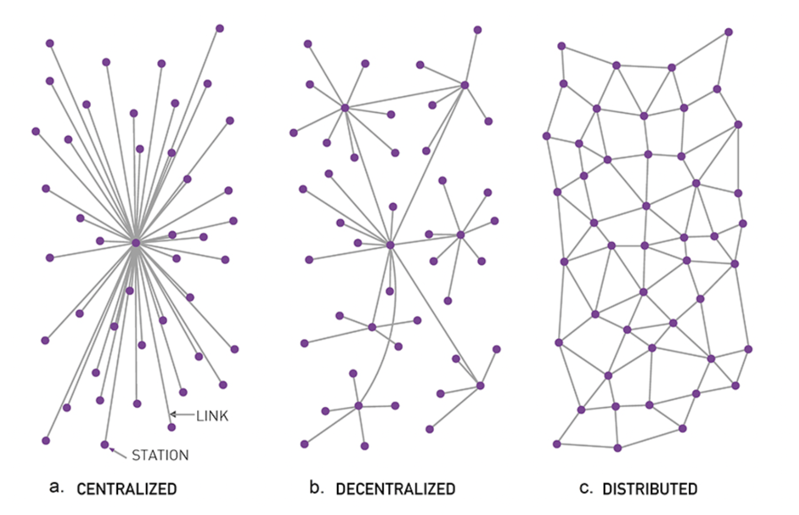
Figure 2. Different types of network structures. Note: This figure illustrates three types of communication networks, borrowed from (Barabási, 2016).

(Campajola et al., 2022) in their paper presents a wide array of indexes to display the different levels of decentralization of Bitcoin, including clustering index, degree distribution, core-periphery structure, etc. In our study, we introduce various network measures to capture the differences between these network features in the token networks of Aave. The first thing to note is that in Figure 2, the network consists of only one component, that is, all nodes are connected by direct or indirect paths. In our transaction data, however, the network consists of many disconnected components. In an ideally centralized market, all nodes should be connected to a single hub; thus the number of components should be one. In a very fragmented market, in contrast, we may observe many components. This argument leads to our first measure of centralization: the number of components (disconnected parts in the network) shows how centralized or fragmented the network is. We compute this measure for every day observed in the data.

The second related measure is the relative size of the largest (giant) component. If the network is more centralized, we expect the largest component to cover a high fraction of nodes, in a fragmented network we observe many small components. We calculate the size of the giant component divided by the total number of nodes in the daily transaction network; the larger this value is, the more centralized the network.

A related measure is the modularity score (formally defined in Table 1) which measures the strength of division of a network into small groups (Newman 2006). A market structure with lower modularity is more centralized, which means that there are no separate communities in the transaction network. This measure can be applied to both connected and disconnected graphs.

Fourth, we capture the characteristics of the structures in Figure 2 by computing the standard deviation of the number of neighbors (degree) in the network. In a centralized network, we have the largest disparity in degree, while in the distributed case, the degree distribution is equal.

Last but not least, we use the concept of core-periphery networks to measure the degree of centralization. In a core-periphery network, a limited number of core members constitute a densely connected hub that are connected to each other and to the peripheral nodes. The peripheral nodes are not connected to each other, only the core members. Note that the centralized structure in the left panel of Figure  2 corresponds to a core-periphery structure with one core member, and the decentralized structure to a core-periphery network with multiple core members. The distributed network in the right panel is not a core-periphery network.

Based on these arguments, we run statistical tests to detect the core-periphery structure in the data, comparing it to a random network with the same degree distribution (KOJAKU, 2022). Our first measure of decentralization is the significance level of this test, which we convert to a binary measure. This measure is equal to 1 when the p-value of the test is less than 0.05, which indicates the presence of a core-periphery structure. In the other case, when the p-value is larger than 0.05, the measure takes the value 0, which indicates that the presence of a core-periphery structure can be rejected.

In addition, for the days when a core-periphery structure describes the data well, we measure the number and degree of core members in the network. In a more centralized network, the number of core members is lower and each core member has a larger degree.

Table 1 summarizes the network measures that we use to capture market centralization in the data.

Table 1. Major Network Features. Note: This table gives the general definitions of the network features included in our study with an explanation and equation.

Name	Definition
num_nodes	Number of unique addresses in the daily transaction network.
num_edges	Number of transactions in the daily transaction network.
Components_cnt	The various disconnected parts of the network, where there is no path that can connect from a node in one component to a node in another component. Components_cnt here refers to the number of components in the daily transaction network
giant_com_ratio	Size of the giant component divided by the total number of nodes in the daily transaction network.
DCstd	Standard deviation of degree centrality. Degree centrality measures the number of neighbors one node has: the higher the number, the more central the node is.
Modularity	Measure of the strength of a network divided into modules. A network with a high degree of modularity has dense connections between nodes within a module but sparse connections between nodes in different modules.
cp_test_pvalue	P value of the significance test of the core-periphery structure.
cp_significance	1 if cp_test_pvalue is less than 0.05 and, else 0 otherwise.
core_cnt	Number of nodes in the core based on the BE core-periphery structure algorithm in the daily transaction network.
avg_core_neighbor	the Average number of neighbors (degree) of the core nodes detected by the core-periphery structure algorithm in the daily transaction network.

Turning to the economic variables of the market, we focus on two common variables of interest: price and 30-day volatility. We expect market network centralization to affect these outcome variables. Table 2 summarizes the economic variables.

Table 2. Major Economic Variables. Note: This table gives the general definitions of the economic variables used as dependent variables in regressions.

Name	Definition
PriceUSD	Fixed closing price of the asset in USD.
VtyDayRet30d	Volatility over 30 days, measured as the standard deviation of the natural log of daily returns over the past 30 days.

4. Data Querying, Mechanics, and Processing

4.1. Data Source

Our data are from three open sources: general economic variables of the AAVE token from Coinmetrics (Coinmetrics, 2022), TVL in Aave from DeFi Pulse (Pulse, 2022), and blockchain transaction records of AAVE token from Bigquery public datasets on the Ethereum blockchain (Bigquery, 2022), ranging from Oct. 10, 2020, to Jul. 30, 2023. Our processed datasets for analysis are at a daily level. We include a detailed dataset overview and dictionary for each dataset in Section A in the Appendix.

4.2. Data Generating Mechanics Explained in AAVE Token Functions

In our network analysis of the AAVE token transfers on the Ethereum blockchain, we define the nodes and edges as follows:

• Nodes: In our network, nodes represent the addresses involved in AAVE token transactions. These addresses can be either the sender or receiver in a transfer of AAVE tokens.

• Edges: The edges in our network are the token transfers themselves. Each edge denotes a transfer of AAVE tokens from one address (node) to another.

This framework allows us to analyze the transaction network of AAVE, providing insights into the flow and distribution of tokens between various participants in the ecosystem.

There are two main types of AAVE token transfers on the Ethereum blockchain:

1. Internal Transfers: These transfers occur between addresses within the Aave protocol. Examples include a user transferring AAVE tokens from their wallet to the Aave protocol as collateral or the Aave protocol transferring AAVE tokens to a user as a reward. Internal transfers are typically faster and cheaper as they do not require gas fees to be paid to the Ethereum network.

2. External Transfers: These transfers occur between addresses outside of the Aave protocol, such as transferring AAVE tokens between wallets or from an exchange to a user’s account. External transfers can be slower and more expensive due to the required gas fees.

Specific types of AAVE token transfers include:

• Lending:

  • Deposit: Users deposit AAVE tokens into the protocol as collateral to borrow other assets.

  • Withdrawal: Users withdraw assets from the lending pool by burning their AAVE tokens.

  • Borrow: Users borrow assets using AAVE tokens as collateral.

  • Repay: Borrowers repay loans, returning assets to the lending pool.

  • Liquidation: If a loan is not repaid, the collateral can be liquidated.

• Staking:

  • Stake: Users stake AAVE tokens to earn rewards.

  • Unstake: Users remove their tokens from the staking pool.

• Governance:

  • Proposing: Suggesting changes to the AAVE protocol.

  • Voting: Casting votes on proposals related to the AAVE protocol.

• Exchange:

  • Transfer: Transferring AAVE tokens between addresses.

  • Swap: Swapping AAVE tokens for other assets.

These are the main examples of the many types of AAVE token transfers that can occur on the Ethereum blockchain, depending on the features of the Aave protocol and the Ethereum network. 

4.3. Data Processing Workflow

4.3.1. Calculate network features

Using the Python NetworkX package (Hagberg et al., 2008), we build daily transaction network graphs using from_address, to_address as nodes and the values as weights. We consider an undirected network between the addresses with weights equal to the total value of transactions between the accounts. This means that we add the transaction values between two duplicate accounts without considering the direction before network building. Based on the daily network, we calculate 24 network features using the NetworkX algorithms (Hagberg et al., 2008), given in Appendix A. We keep only the network features listed in Table 1 to answer the research questions of this paper but open source the rest for future research.

4.3.2. Extract the core-periphery structure

To extract the core-periphery structure, we utilize the Python cpnet package (KOJAKU, 2022), which contains algorithms implemented in Python for detecting core-periphery structures in networks. cpnet.BE (KOJAKU, 2022) is the algorithm used for the Borgatti-Everett (BE) algorithm, which, identifies nodes either as either core or periphery in a single group (Borgatti and Everett, 2000). cpnet.KM_config (KOJAKU, 2022) is used for examining multiple pairs of core-periphery nodes, which can return the coreness and pair of each node. This package also allows us to conduct significance testing via the q-s test on the core-periphery structure of the daily network to assess the fitness of this algorithm for our data, where we use 0.05 as the significance level. The core-periphery structure detected for the input network is considered significant if it is stronger than those detected in randomized networks (Kojaku and Masuda, 2018b). We calculate the number of cores and the average number of neighbors of the core nodes to further investigate the levels of decentralization given the core-periphery structure. Additionally, based on the daily networks constructed using the core-periphery algorithm, we record all core addresses that appear during the period and the number of days that they become core. The type (contract or address) and information links of those cores are extracted from Etherscan.io (etherscan.io, 2019) and recorded for further comparison.

4.3.3. Analyze interactions with economic variables

Among the economic metrics queried as shown in Appendix B, the price in USD PriceUSD, 30-day volatility VtyDayRet30d and total value locked (TVL) in USD tvlUSD are chosen as the dependent variables in our regression models since they are significant and commonly used economic metrics in market valuation. Specifically, the price intuitively reflects the market value of the AAVE token, which is perfectly correlated with the market capitalization for the Aave protocol during the time range of our data. The 30-day volatility can reflect the degree of volatility in the token market over the past month and the potential existence of risks or tendencies (Coinmetrics, 2022). The total value locked, which is the overall value of crypto assets deposited in the Aave protocol in USD (George, 2022), is a unique economic metric in the context of the cryptocurrency market. Furthermore, before regression, we need to ensure stationarity of time-series data-that is, that the mean, variance, and autocorrelation structure remain constant over time (Brownlee, 2017), and the values give an approximately normal distribution. We transform the variables using methods including differencing the data and taking the logarithm difference, or percentage change based on the Dickey-Fuller test results to ensure that they become stationary. After that, we scale all the stationary variables between 0 and 1 for scale comparison and test the correlation for all the independent variables (after transformation) to avoid high correlation in the regressions.

5. Empirical Analysis Methods and Results

5.1. The realization of decentralization (the core-periphery structure)

5.1.1. Construct core-periphery structures

As introduced and discussed in the previous sections, we apply the Borgatti-Everett (BE) algorithm (Borgatti and Everett, 2000) and the multiple-pairs core-periphery structure algorithm (Kojaku and Masuda, 2018b) to the AAVE transaction network to investigate whether the daily graphs can be separated into dense transactions between some active addresses (defined as the core) and some other loose transactions between some small addresses (defined as the periphery) in either a single pair or multiple pairs. In this section, we connect the properties of the core-periphery structure in the AAVE transaction network with the real functions and types of the specific addresses (some typical addresses) to further explore the question of centralization vs. decentralization.

We test the significance of all 365 observations. The results indicate that the AAVE daily transaction network is insignificant in the multiple-pair core-periphery structure, but partially significant in the one-pair structure with 232 significant (64%) and 133 insignificant (36%) days. Comparing the distribution (displayed in Figure 3) of the number of nodes in the core and the average number of degrees of the core nodes (described in Table 1) in the significant and nonsignificant daily graphs that we tested, we find that the number of nodes in the core in the significant graph is much smaller. The average number of neighbors of the core nodes is more prominent in those significant graphs and vice versa. By interpretation, when the transaction network significantly fits the core-periphery structure, it can be divided into small groups of denser and looser connections. The transaction difference between nodes is larger; thus, the degree of centralization is greater. In this case, a few addresses are likely to dominate most transactions.

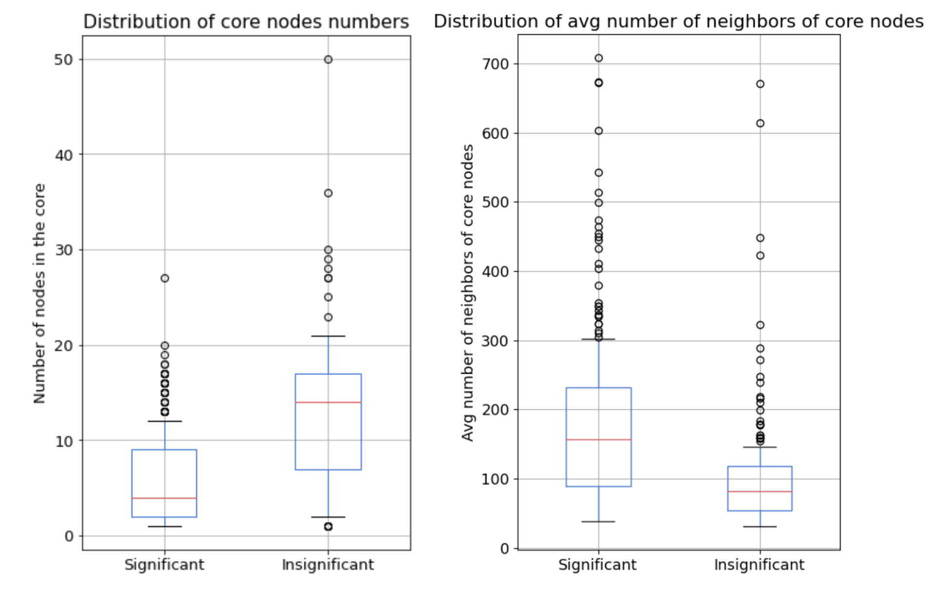
Figure 3. Core-periphery structure features distribution box plots. Note: This figure plots the distribution of the number of core nodes (left panel) and the average number of neighbors of core nodes (right panel) on days with significant (p-value smaller than 0.05) and insignificant core-periphery test results.

To depict the structure and comparison in a more intuitive and explainable way, we pick two representative days of the significant and nonsignificant graph to visualize the network, as displayed in Figure 4. It shows the core-periphery network graphs of transactions among the identified core accounts based on the cpnet.BE algorithms in a spiral layout on 2020-10-12 (left panel) and 2021-02-22 (right panel), where the dark dots represent the core nodes and the light dots are the periphery nodes. The two panels clearly illustrate that on a significant core-periphery graph (left panel), all core nodes are closely linked, and each core node forms an aggregation group with periphery nodes (each with a high degree) so that any two nodes can connect in a few steps. The overall network structure of the transactions among the identified core accounts is very compact and cohesive, resulting in a significant core-periphery structure, which is also more centralized in the transaction since the core nodes are dominant. In contrast, the right panel shows a looser overall connection. Each identified core node has a smaller degree, with many scattered periphery nodes; some nodes require a long step size to connect to other nodes, which prevents the structure from being significantly certified as core-periphery and adds to the level of decentralization in the transaction network.

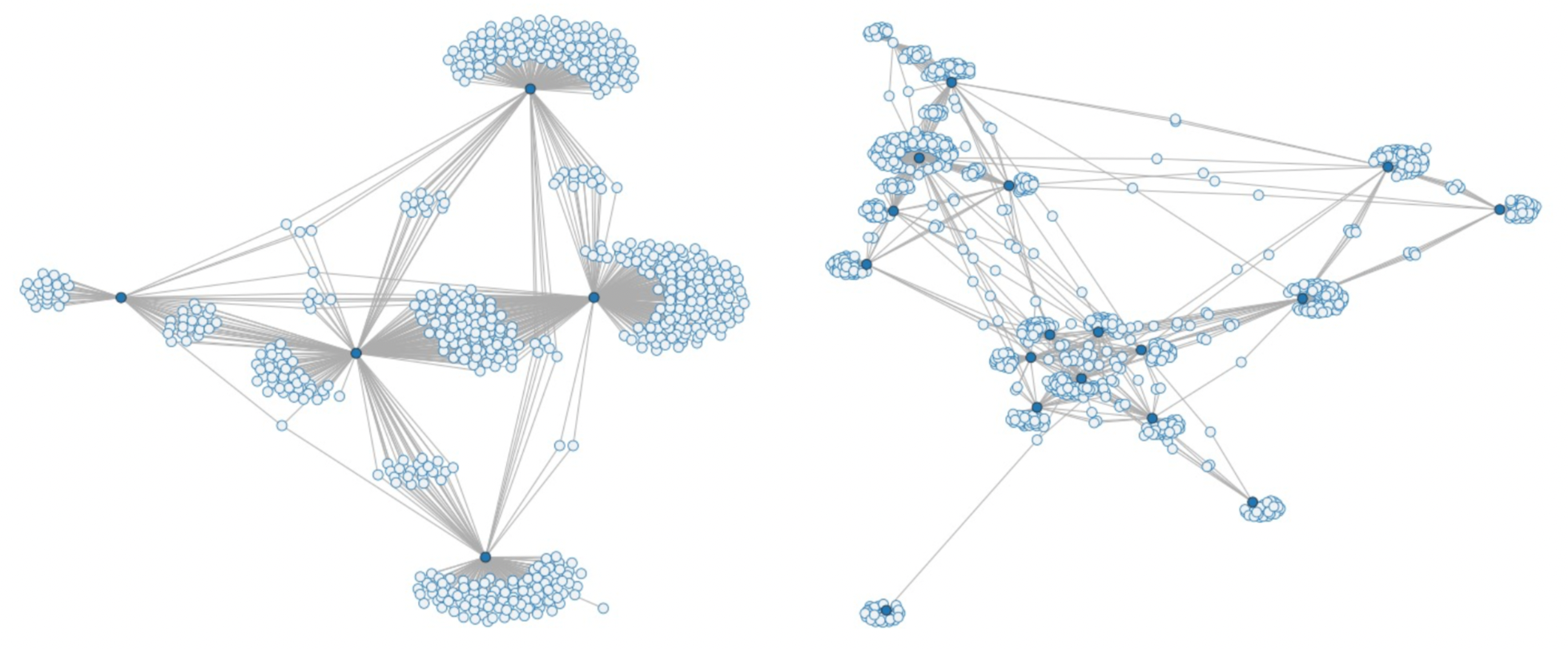
Figure 4. Network graphs on 2020-10-12 (left panel) and 2021-02-22 (right panel). Note: This figure shows the core-periphery network graphs of transactions among the identified core accounts based on the cpnet.BE algorithms in a spiral layout on 2020-10-12 (left panel) and 2021-02-22 (right panel), where the dark dots represent the core nodes and the light dots are the periphery nodes. The left panel returns a. significant p-value in the significance test, while the right panel is nonsignificant.

5.1.2. Compare the core-periphery structure for externally owned and contract account

Furthermore, we investigate addresses/accounts that were once identified as core members in the graphs. There are two types of accounts defined on Ethereum: externally owned accounts (EOAs) and contract accounts (CAs, also called smart contracts) (Hu et al., 2021). EOAs are created and owned by users with a private key set and can be utilized to deposit and transfer assets and call smart contracts (Hu et al., 2021). The CAs are execution programs composed of smart contract code, which also possesses asset balance and will be automatically executed if the trigger condition in met (Szabo, 1997). We record the accounts that appear to be identified as core nodes during the period and the number of days that they become core, based on the daily networks constructed by the Borgatti-Everett (BE) algorithm (Borgatti and Everett, 2000). We extract the type of account (EOA or CA) according to Etherscan.io (etherscan.io, 2019).

Figure 5 plots the distribution of the number of core days for EOAs and CAs. From the graph, the range of day counts is generally larger for the contract accounts, where the extreme value is much larger than its counterpart for externally owned accounts. The four outliers identified (two for CA and two for EOA) appear to be in the core for many of the days, resulting in a centralized transaction that could significantly affect the level of decentralization. We investigate the detailed account information of these four accounts by Etherscan.io (etherscan.io, 2019) for further explanation.

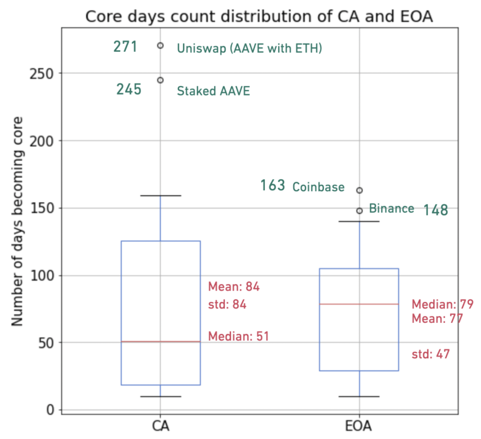
Figure 5. Core day count distribution box plots. Note: This figure plots the distribution of the number of core days for EOAs and CAs, where the y-axis is the number of days in which the node is in the core.

The two outliers among EOAs are Binance and Coinbase, which are the two top centralized exchanges in the cryptocurrency market. A centralized exchange is a significant online platform for users to buy and sell cryptocurrencies, offering security and monitoring for the individual to complete the transaction in a trustworthy environment (Reiff, 2019). Due to the popularity of these two centralized exchanges, a tremendously large number of transfers occur through these two accounts daily between the same and different types of cryptocurrencies by many EOAs. Given the results of the core-periphery structure, the centralized exchange exerts a significant influence on the AAVE daily transaction network and brings a high level of “centralization” to it.

The two outliers among CAs are decentralized exchanges, we find that one of them is an automated market maker on Uniswap, a decentralized exchange for transactions between AAVE and Ether. Automated market makers (AMMs), first introduced by Hanson’s logarithmic market scoring rule (LMSR) (Hanson, 2003), are contracts that allow liquidity to be automatically provided to the crypto market automatically (Fritsch and Zürich, 2021). Based on the AMM, this contract is built on Uniswap, which allows agents to trade between AAVE and Ether at the price and rates specified by the pricing function, and the price is kept enormous centered transaction network around this account, which greatly influences the core-periphery structure and increases the centralization of the AAVE transaction graph. Another is the smart contract of Stated AAVE, which performs the functions in the Aave decentralized bank of staking (moving assets to long-term saving account), redeeming (getting collateral back), getting rewards (claiming interest rates), etc. (Whitepaper.io, 2020).

On the one hand, the two outliers of centralized exchanges put the promise of blockchain decentralization in doubt; on the other hand, the two outliers of decentralized exchanges evidence that blockchain can mitigate the dependence on trusted centralized entities.

5.2. Blockchain network dynamics and correlations

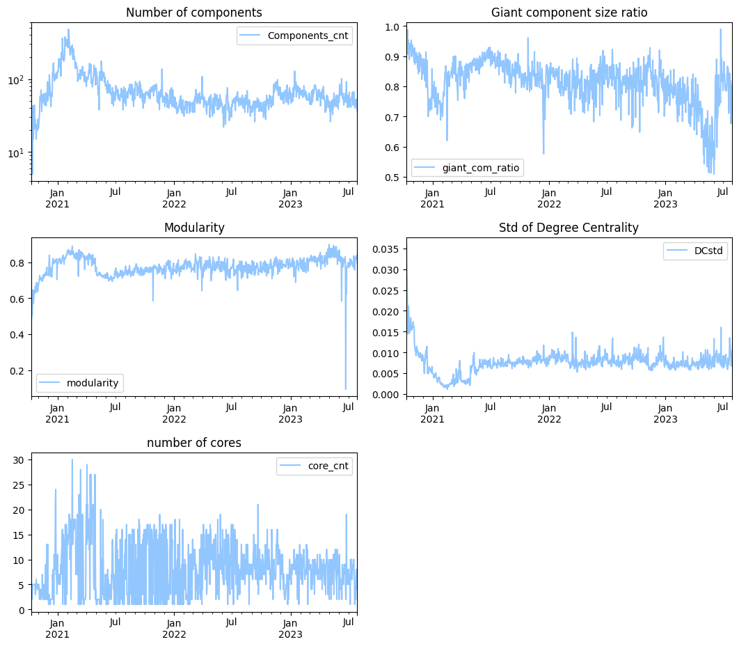
Figure 6. Time-series plots of network features. Note: This figure gives time-series plots of network features included in our study, with the feature name in the title of each panel.

In addition to the core-periphery structure, we use other network properties to capture market centralization. We find that all the intertemporal network features indicate consistent dynamics whereby the AAVE token transaction network first becomes more decentralized and then reverts to being more centralized.

5.2.1. Numbers of components

When the market is more centralized, we expect to have fewer components in the network since most transactions go through a central node that connects most nodes indirectly, forming a network component. The left upper panel of Figure 6 plots the number of components over time. The graph suggests that the AAVE market first became increasingly decentralized, as indicated by the increase in the number of components up to February 2021, and then showed a tendency to centralize as the number of components increased. The network structure of the market converged to approximately 100 components after July 2021.

5.2.2. Giant component size ratio

A related network property is the relative size of the giant component. In a centralized market, the giant component covers a large fraction of the nodes, while in a decentralized market, the giant component is relatively small. The lower right panel of Figure 6 shows that the relative size of the giant component first decreased and then increased. This again suggests that the market was initially decentralized and then became more centralized.

5.2.3. Modularity score

The modularity score is small when the market is centralized, meaning that there are no separate communities in the network. In contrast, in a decentralized market, many communities are not or are only weakly connected to each other, implying a high modularity score. The right upper panel of Figure 6 shows the evolution of modularity. The modularity score increased first, indicating a tendency to decentralize, and then it started to decrease, suggesting centralization.

5.2.4. The standard deviation of degree centrality

The standard deviation of degree centrality is large (small) when the market is centralized (decentralized) since, in a centralized market, a few hubs have a high degree while the other nodes have only a few connections. In the right middle panel of Figure 6, we see that the standard deviation of degree centrality first decreased and then increased, suggesting that the market first showed a tendency toward decentralization and then toward centralization.

Figure 7. Correlation heatmap of network features. Note: This figure plots the correlation between network features, red represents a positive correlation while blue represents a negative correlation. The depth of the color is proportional to the correlation coefficient value.

5.3. The impact of network features on market return and volatility

5.3.1. Background and Methods

Liu and Tsyvinski (2018)’s study demonstrated that there is strong evidence of time-series momentum at various time horizons of the cryptocurrency network features; this evidence could potentially indicate a momentum effect of the network on DeFi economic metrics. We utilize the Python package smf.ols for the OLS regression to test the following two hypotheses:

• Return of Investment (ROI): The decentralization level measured by network features predicts higher future ROI.

• Market Volatility Growth Rate (MVGR): The decentralization level measured by network features predicts a lower increase in volatility.

We utilize Python smf.ols for the OLS regressions with return (ROI) to test the two hypotheses. We generate the results for ROI and MVGR at different windows from one-day, one-week, to nighty-day horizons. Each dependent variable is regressed on each of the network features and control variables. To avoid the issues of heterogeneity and autocorrelation, we generalize the regressions with Newey-West estimators (Liu and Tsyvinski, 2018).

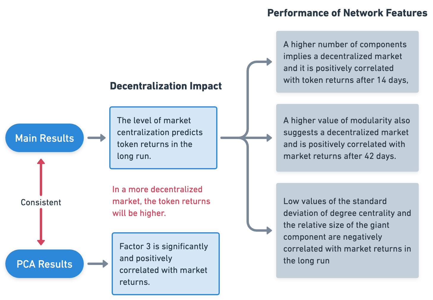
Figure 8. Results of the token market returns (USD).Note: This figure reports the results of predicting the token market returns (USD) using the 7-day moving average of network variables.

5.3.2. Results on market returns

Figure 8 displays the outcomes of our analysis on token market returns (in USD), utilizing a 7-day moving average of network variables. Detailed regression results are provided in Table 4 and Table 5 in the Appendix. Upon examining token market returns, we observe a notable correlation: a higher degree of market decentralization appears to be a predictive factor for long-term token returns. Specifically, in markets characterized by greater decentralization, token returns tend to be more substantial. This finding aligns with the prevalent expectation among stakeholders that a blockchain’s value increases with its decentralization. For instance, a more decentralized transaction network in DeFi tokens correlates with optimistic stakeholder projections about future returns, culminating in a self-reinforcing equilibrium of enhanced returns.

Our regression analyses, centered on network attributes, corroborate this trend. We note a significant and positive correlation between the number of network components—a marker of decentralization—and token returns after a 14-day period. Similarly, an elevated modularity value, indicative of market decentralization, demonstrates a significant and positive association with market returns over a 21-day span.

In contrast, lower values in the standard deviation of degree centrality and the relative size of the largest network component, both indicative of decentralization, exhibit a significant and negative correlation with long-term market returns. Additionally, the core-periphery structure’s significance, representative of a centralized network, bears a negative correlation with market returns for most periods exceeding 7 days.

It is crucial to note the high volatility of short-term market returns, which renders our network measures less predictive in this timeframe. This observation is mirrored in the R-squared values of our regressions: they approach zero for short-term forecasts but increase with longer time horizons. The premise that short-term returns of cryptocurrency tokens are less predictable by network features is in agreement with the findings of Liu et al. (2022) (Liu and Zhang, 2022).

PC1 $$=-0.26\times\text{Components\_cnt}+0.87\times\text{giant\_com\_ratio}$$

(1) $$\quad-0.32\times\text{modularity}+0.26\times\text{DCstd},$$

PC2 $$=0.78\times\text{Components\_cnt}+0.41\times\text{giant\_com\_ratio}$$

(2) $$\quad+0.08\times\text{modularity}-0.47\times\text{DCstd},$$

PC3 $$=0.56\times\text{Components\_cnt}-0.19\times\text{giant\_com\_ratio}$$

(3) $$\quad-0.43\times\text{modularity}+0.68\times\text{DCstd}.$$

To further substantiate our results, we employed principal component analysis (PCA) to distill the essence of the five network features representing centralization measures. The PCA formulas are presented in the collection of Equations 1, 2, 3. The optimal number of factors was determined by maximizing the variance explained by these features. In our regression outputs, we found Factor 3, which quantifies decentralization, to be significantly and positively correlated with market returns. This reaffirms our earlier observations: a heightened level of decentralization is consistently associated with increased market returns.

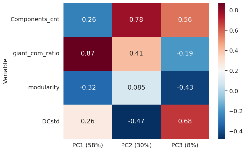
Figure 9. Interpretation of PCA. Note: This figure depicts the correlation coefficient between the original variables and the components. Positive and negative values in the graph reflect the positive and negative correlation of the variables with the PCs. Red represents a positive correlation, blue represents a negative correlation, and the depth of the color is proportional to the correlation coefficient value.

5.3.3. Results on market volatility

In our examination of market volatility, as depicted in Figure 10, we conducted a parallel analysis, the results of which are detailed in Table 6 and Table 7 in the Appendix. Our findings indicate a discernible positive correlation between the degree of decentralization and the growth rate of market volatility. Specifically, an increase in the number of network components, a proxy for market decentralization, is significantly and positively correlated with future market volatility, particularly for mid-range horizons of 42, 49, and 56 days. This observation suggests that markets with higher levels of decentralization are prone to increased volatility. Interestingly, this result aligns with the theoretical expectation that decentralized markets should exhibit lower volatility, as the impact of market shocks tends to be more dispersed in such environments.

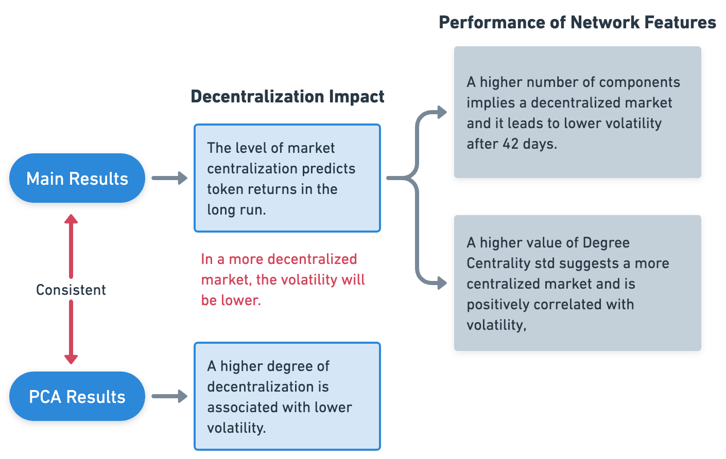
Figure 10. Results of the 30-day volatility growth rate. Note: This figure reports the results of predicting the 30-day volatility growth rate using the 7-day moving average of network variables.

6. Conclusions and Discussion

6.1. Extensions in three facets

Our study shows that social network analysis is instrumental in characterizing the level, dynamics, and impacts of decentralization in DeFi token transactions. Our research is also seminal in terms of inspiring future research on the three facets of application scenarios, research questions, and methodology.

1. Application Scenarios. Our methods can be generally applied to transaction tokens issued by other DeFi protocols, such as decentralized payment, exchange, assets, derivatives and even non-financial applications on blockchains. 

2. Research Questions. We can extend our analysis to study the interplay of other network features and economic variables. For example, one straightforward follow-up research is to extend the analysis to include other network features for which we have provided open-source data as defined in Appendix A.

3. Methodology. We can further explore the interplay of network dynamics and token economics by causal inference through advanced econometrics and prediction algorithms in machine learning (Athey, 2015).

6.2. On the mechanics of blockchain decentralization

Is decentralized finance actually decentralized? The answer from our pioneering blockchain network study is intriguing. We found that the current research on decentralization tends to neglect two important aspects of the mechanics of blockchain decentralization:

1. How do incentives affect agents’ behavior in transaction network formations?

2. How do incentives affect the final realizations of network decentralization?

These two gaps neglections in the literature leave a door for future research to improve the mechanism to support a truly decentralized economy. Why? The blockchain infrastructure only provides the possibility for peer-to-peer transactions. However, the actually realized decentralization of blockchain transaction networks depends on the behavior of stakeholders, who are affected by incentives. If we can better understand the incentives that govern the stakeholders’ behavior and the formation of transaction networks, we can design incentives schemes to support desired levels of decentralization.  Future research can experiment with other scientific methods of theoretical modeling and simulations. For example, we can further apply network game theory (Azouvi and Hicks, 2020) to distributed systems to study how incentives affect agents’ strategic behaviors and the transaction network formations on the blockchain. We can also apply agent-based modeling (Iori and Porter, 2012) to simulate the transaction networks on blockchain to systematically evaluate the effect of incentive design changes.

Appendix A Network Features

Table 3. Network Features. Note: This table gives the general definitions of all network features calculated in our study with the explanation.

Name	Definition
num_nodes	Number of unique addresses in daily transaction network.
num_edges	Number of transactions in daily transaction network.
Degree mean	The number of edges a node has, an average of nodes.
Degree std	The number of edges a node has the standard deviation of nodes.
Top10Degree mean	Average degree of the addresses with top 10 highest degree values during the whole period.
Top10Degree std	Standard deviation of the degree of the addresses with the top 10 highest degree values during the whole period.
Top10 Degree mean ratio	Top 10 addresses’ degree mean divided by the general degree mean.
Relative degree	Network density. The portion of the potential connections in a network is actual connections.
DCmean	The average value of degree centrality.
DCstd	The standard deviation of degree centrality.
Cluster_mean	Mean of clustering coefficient. The degree to which nodes in a graph tend to cluster together.
Cluster_std	Standard deviation of clustering coefficient. The degree to which nodes in a graph tend to cluster together.
Modularity	Modularity is a way to measure the strength of a network divided into modules. A network with a high degree of modularity has dense connections between nodes within a module, but sparse connections between nodes in different modules.
Transitivity	Transitivity is the overall probability for the network to have adjacent nodes interconnected, thus revealing the existence of tightly connected communities.
eig_mean	Mean of eigenvector centrality. Measures the degree to which the division of a network into communities.
eig_std	Standard deviation of eigenvector centrality. Measures the degree to which the division of a network into communities.
closeness_mean	Mean of closeness centrality. The reciprocal of the farness.
closeness_std	Standard deviation of closeness centrality. The reciprocal of the farness.
giant_com_ratio	Size of the giant component divided by the total number of nodes in the daily transaction network.
Components_cnt	The components of the network are the various disconnected parts, where there is no path that can connect from a node in one component to a node in another component. Components_cnt here refers to the number of components in the daily transaction network
cp_test_pvalue	P-value of the significant test of the core-periphery structure.
cp_significance	1 if cp_test_pvalue is less than 0.05, else 0.
core_cnt	Number of nodes in the core based on the BE core-periphery structure algorithm in the daily transaction network.
avg_core_neighbor	the Average number of neighbors (degree) of the core nodes detected by the core-periphery structure algorithm in daily transaction network.

Table 3 contains 24 daily network features calculated from the AAVE transaction data we calculated using the NetworkX package, which can be used as a reference for further network studies.

Appendix B Supplementary Regression Table

Table 4. Results of the token market returns (USD). Note: This table reports the results of predicting the future market return (USD) using the 7-day moving average of network variables. Columns (1)-(10) represent one day, one week to eight weeks, and 90 days respectively. *, **, and *** denote significance at the 10%, 5%, and 1% levels. The data frequency is daily. The residual standard errors are reported in parentheses.

Time horizon	t, t+1	t, t+7	t, t+14	t, t+21	t, t+28	t, t+35	t, t+42	t, t+49	t, t+56	t, t+90
	(1)	(2)	(3)	(4)	(5)	(6)	(7)	(8)	(9)	(10)
$\vartriangle$ component cnt	-0.034	0.125	0.247**	0.384***	0.323***	0.301***	0.234**	0.261**	0.289**	0.233***
$R^{2}$	0	0.006	0.018	0.032	0.028	0.027	0.016	0.018	0.018	0.013
Residual Std. Error	(0.105)	(0.100)	(0.120)	(0.138)	(0.123)	(0.119)	(0.122)	(0.125)	(0.138)	(0.134)
$\vartriangle$ giant com ratio	0.005	-0.039	-0.060*	-0.065*	-0.062*	-0.040	-0.044	-0.099*	-0.129**	-0.083***
$R^{2}$	0	0.002	0.003	0.003	0.003	0.001	0.002	0.008	0.011	0.005
Residual Std. Error	(0.105)	(0.101)	(0.120)	(0.140)	(0.125)	(0.120)	(0.123)	(0.126)	(0.139)	(0.135)
$\vartriangle$ log(modularity)	0.008	0.057	0.127	0.191	0.201	0.142	0.158**	0.203**	0.195**	0.279***
$R^{2}$	0	0	0.001	0.001	0.002	0.002	0.009	0.015	0.016	0.035
Residual Std. Error	(0.105)	(0.101)	(0.121)	(0.140)	(0.125)	(0.120)	(0.122)	(0.125)	(0.139)	(0.133)
$\vartriangle$ log(DCstd)	0.012	-0.041	-0.097**	-0.178***	-0.207***	-0.161***	-0.153***	-0.186**	-0.189**	-0.241***
$R^{2}$	0	0	0.004	0.016	0.028	0.018	0.016	0.022	0.018	0.032
Residual Std. Error	(0.105)	(0.101)	(0.120)	(0.139)	(0.123)	(0.119)	(0.122)	(0.125)	(0.138)	(0.133)
cp significance	-0.014	-0.090**	-0.163***	-0.278***	-0.322***	-0.324**	-0.314*	-0.188	0.056	1.834***
R2	0.007	0.031	0.039	0.061	0.046	0.028	0.018	0.005	0	0.124
Residual Std. Error	(0.080)	(0.242)	(0.391)	(0.528)	(0.718)	(0.931)	(1.138)	(1.269)	(1.351)	(2.432)
PCA component1	-0.015	-0.027	-0.018	0.007	0.002	0.006	0.012	0.018	0.062	0.327***
PCA component2	0.046	0.091*	0.128*	0.144*	0.115*	0.097	0.076	0.062	0.057	-0.067
PCA component3	0.046	0.159***	0.275***	0.378***	0.305***	0.277***	0.262***	0.277***	0.322***	0.558***
$R^{2}$	0.005	0.045	0.083	0.105	0.087	0.076	0.060	0.060	0.064	0.252
Residual Std. Error	(0.105)	(0.098)	(0.116)	(0.133)	(0.120)	(0.116)	(0.119)	(0.122)	(0.135)	(0.117)

Table  4 gives the regression result table of the token market returns (USD).

Table 5. Results of the token market returns (USD) with control variable. Note: This table reports the results of predicting the future market return (USD) using the 7-day moving average of network variables with Eth price as a control variable. Columns (1)-(10) represent one day, one week to eight weeks, and 90 days respectively. *, **, and *** denote significance at the 10%, 5%, and 1% levels. The data frequency is daily. The residual standard errors are reported.

Time horizon	t, t+1	t, t+7	t, t+14	t, t+21	t, t+28	t, t+35	t, t+42	t, t+49	t, t+56	t, t+90
	(1)	(2)	(3)	(4)	(5)	(6)	(7)	(8)	(9)	(10)
$\vartriangle$ component cnt	-0.046	0.095	0.197**	0.316***	0.258***	0.236***	0.164**	0.183*	0.199*	0.146***
ETHPriceUSD	-0.046***	-0.110***	-0.182***	-0.249***	-0.234***	-0.235***	-0.252***	-0.274***	-0.318***	-0.308***
Adjusted R2	0.008	0.064	0.13	0.189	0.205	0.22	0.231	0.261	0.287	0.29
Residual Std. Error	(0.105)	(0.097)	(0.112)	(0.126)	(0.111)	(0.106)	(0.108)	(0.108)	(0.118)	(0.114)
$\vartriangle$ giant com ratio	0.007	-0.033	-0.05	-0.052	-0.05	-0.027	-0.028	-0.081*	-0.104**	-0.058**
ETHPriceUSD	-0.045***	-0.112***	-0.186***	-0.255***	-0.239***	-0.240***	-0.255***	-0.277***	-0.320***	-0.310***
Adjusted R2	0.007	0.002	0.003	0.003	0.003	0.001	0.002	0.008	0.011	0.005
Residual Std. Error	(0.105)	(0.097)	(0.113)	(0.128)	(0.113)	(0.107)	(0.108)	(0.109)	(0.118)	(0.114)
$\vartriangle$ log(DCstd)	0.024	-0.011	-0.047	-0.109**	-0.142***	-0.095**	-0.082*	-0.109*	-0.096	-0.151***
ETHPriceUSD	-0.046***	-0.112***	-0.184***	-0.250***	-0.232***	-0.235***	-0.251***	-0.272***	-0.317***	-0.302***
Adjusted R2	0.008	0.061	0.121	0.174	0.199	0.21	0.228	0.26	0.283	0.297
Residual Std. Error	(0.105)	(0.097)	(0.113)	(0.127)	(0.112)	(0.107)	(0.108)	(0.108)	(0.118)	(0.113)
$\vartriangle$ log(modularity)	-0.011	0.011	0.052	0.088	0.105	0.057	0.076	0.117*	0.105	0.192***
ETHPriceUSD	-0.045***	-0.112***	-0.186***	-0.256***	-0.239***	-0.240***	-0.253***	-0.274***	-0.318***	-0.302***
Adjusted R2	0.007	0.061	0.119	0.168	0.187	0.204	0.226	0.257	0.283	0.301
Residual Std. Error	(0.105)	(0.097)	(0.113)	(0.128)	(0.113)	(0.107)	(0.108)	(0.109)	(0.118)	(0.113)
PCA component1	-0.011	-0.019	-0.004	0.026	0.02	0.025	0.027	0.035	0.082**	0.339***
PCA component2	0.046	0.092*	0.129**	0.146*	0.117*	0.098*	0.077	0.063	0.058	-0.071*
PCA component3	0.031	0.124**	0.217***	0.297***	0.227***	0.197***	0.173***	0.180***	0.208***	0.450***
ETHPriceUSD	-0.042***	-0.100***	-0.167***	-0.231***	-0.220***	-0.224***	-0.242***	-0.264***	-0.308***	-0.286***
Adjusted R2	0.009	0.09	0.173	0.235	0.237	0.244	0.251	0.278	0.308	0.484
Residual Std. Error	(0.105)	(0.096)	(0.110)	(0.123)	(0.109)	(0.105)	(0.106)	(0.107)	(0.116)	(0.097)

Table  5 gives the regression result table of the token market returns (USD) with the control variable.

Table 6. Results of the 30-day volatility growth rate. Note: This table reports the results of predicting the 30-day volatility growth rate using the 7-days moving average of network variables. Columns (1)-(10) represent one day, one week to eight weeks, and 90 days respectively. *, **, and *** denote significance at the 10%, 5%, and 1% levels. The data frequency is daily. The residual standard errors are reported in parentheses.

Time horizon	t, t+1	t, t+7	t, t+14	t, t+21	t, t+28	t, t+35	t, t+42	t, t+49	t, t+56	t, t+90
	(1)	(2)	(3)	(4)	(5)	(6)	(7)	(8)	(9)	(10)
$\vartriangle$ component cnt	-0.051	-0.059	-0.026	-0.069	-0.113	-0.132	-0.218***	-0.393***	-0.423***	-0.186
$R^{2}$	0.002	0.002	0	0.001	0.002	0.002	0.006	0.014	0.016	0.004
Residual Std. Error	(0.078)	(0.082)	(0.121)	(0.134)	(0.161)	(0.178)	(0.184)	(0.220)	(0.221)	(0.194)
$\vartriangle$ giant com ratio	-0.014	-0.008	-0.028	-0.05	-0.042	-0.085	-0.085	-0.078	-0.069	0.044
$R^{2}$	0	0	0.001	0.002	0.001	0.003	0.003	0.002	0.001	0.001
Residual Std. Error	(0.078)	(0.082)	(0.121)	(0.134)	(0.161)	(0.178)	(0.185)	(0.221)	(0.222)	(0.194)
$\vartriangle$ log(DCstd)	0.058**	0.043	0.017	0.005	0.058	0.108	0.126	0.198**	0.148	-0.042
$R^{2}$	0.006	0.003	0	0	0.001	0.004	0.005	0.008	0.005	0
Residual Std. Error	(0.077)	(0.082)	(0.121)	(0.134)	(0.161)	(0.178)	(0.185)	(0.220)	(0.222)	(0.194)
$\vartriangle$ log(modularity)	0	0.027	0.006	-0.001	0.001	0	0.037	0.042	0.026	0.055
$R^{2}$	0	0.001	0	0	0	0	0	0	0	0.001
Residual Std. Error	(0.078)	(0.082)	(0.121)	(0.134)	(0.161)	(0.178)	(0.185)	(0.221)	(0.223)	(0.194)
PCA component1	-0.037	-0.076***	-0.139***	-0.172***	-0.212***	-0.255***	-0.262***	-0.283***	-0.245***	-0.286***
PCA component2	-0.039	-0.062*	-0.099**	-0.123**	-0.140**	-0.156**	-0.113	-0.055	0.078	0.310***
PCA component3	-0.028	-0.091***	-0.167***	-0.215***	-0.268***	-0.300***	-0.356***	-0.442***	-0.413***	0.150**
$R^{2}$	0.008	0.036	0.052	0.067	0.071	0.075	0.073	0.066	0.052	0.103
Residual Std. Error	(0.077)	(0.081)	(0.118)	(0.130)	(0.155)	(0.172)	(0.178)	(0.214)	(0.217)	(0.184)

Table  6 gives the regression result table of the 30-day volatility growth rate.

Table 7. Results of the 30-day volatility growth rate with control variable. Note: This table reports the results of predicting the 30-day volatility growth rate using the 7-days moving average of network variables with Eth price as a control variable. Columns(1)-(10) represent one day, one week to eight weeks, and 90 days respectively. *, **, and *** denote significance at the 10%, 5%, and 1% levels. The data frequency is daily. The residual standard errors are reported in parentheses.

Time horizon	t, t+1	t, t+7	t, t+14	t, t+21	t, t+28	t, t+35	t, t+42	t, t+49	t, t+56	t, t+90
	(1)	(2)	(3)	(4)	(5)	(6)	(7)	(8)	(9)	(10)
$\vartriangle$ component cnt	-0.048	-0.055	-0.021	-0.065	-0.109	-0.127	-0.212**	-0.384***	-0.408***	-0.144
ETHPriceUSD	0.012	0.012	0.017	0.015	0.016	0.016	0.019	0.033	0.052	0.148***
Adjusted R2	0.001	0.001	-0.001	0	0.001	0.001	0.005	0.013	0.017	0.034
Residual Std. Error	(0.078)	(0.082)	(0.121)	(0.134)	(0.161)	(0.178)	(0.185)	(0.220)	(0.221)	(0.191)
$\vartriangle$ giant com ratio	-0.015	-0.009	-0.029	-0.051	-0.043	-0.087	-0.087	-0.081	-0.074	0.033
ETHPriceUSD	0.013	0.013	0.018	0.017	0.019	0.02	0.026	0.044	0.063	0.151***
Adjusted R2	0	-0.001	0	0.001	0	0.002	0.002	0.002	0.003	0.032
Residual Std. Error	(0.078)	(0.082)	(0.121)	(0.134)	(0.161)	(0.178)	(0.185)	(0.221)	(0.222)	(0.191)
$\vartriangle$ log(DCstd)	0.055**	0.04	0.012	0	0.053	0.104	0.121	0.188*	0.132	-0.089
ETHPriceUSD	0.01	0.011	0.017	0.016	0.015	0.013	0.018	0.032	0.054	0.157***
Adjusted R2	0.004	0.002	-0.001	-0.001	0	0.002	0.003	0.007	0.006	0.034
Residual Std. Error	(0.077)	(0.082)	(0.121)	(0.134)	(0.161)	(0.178)	(0.185)	(0.220)	(0.222)	(0.191)
$\vartriangle$ log(modularity)	0.004	0.032	0.012	0.003	0.006	0.006	0.045	0.054	0.044	0.1
ETHPriceUSD	0.013	0.014	0.018	0.016	0.018	0.019	0.026	0.045	0.064	0.156***
Adjusted R2	-0.001	0	-0.001	-0.001	-0.001	-0.002	-0.001	0	0.002	0.034
Residual Std. Error	(0.078)	(0.082)	(0.121)	(0.134)	(0.161)	(0.178)	(0.185)	(0.221)	(0.222)	(0.191)
PCA component1	-0.038	-0.076***	-0.139***	-0.172***	-0.212***	-0.255***	-0.262***	-0.284***	-0.247***	-0.291***
PCA component2	-0.039	-0.062*	-0.099**	-0.123**	-0.140**	-0.156**	-0.113	-0.055	0.079	0.315***
PCA component3	-0.024	-0.087***	-0.163***	-0.213***	-0.266***	-0.299***	-0.355***	-0.435***	-0.398***	0.221***
ETHPriceUSD	0.012	0.009	0.01	0.005	0.004	0.003	0.004	0.016	0.039	0.185***
Adjusted R2	0.005	0.032	0.049	0.063	0.067	0.071	0.069	0.062	0.05	0.149
Residual Std. Error	(0.077)	(0.081)	(0.118)	(0.130)	(0.155)	(0.172)	(0.178)	(0.214)	(0.217)	(0.179)

Table  7 gives the regression result table of the 30-day volatility growth rate with the control variable.

References

- (1)
- Anand et al. (2013) Kartik Anand, Prasanna Gai, Sujit Kapadia, Simon Brennan, and Matthew Willison. 2013. A network model of financial system resilience. Journal of Economic Behavior & Organization 85 (01 2013), 219–235. https://doi.org/10.1016/j.jebo.2012.04.006
- Athey (2015) Susan Athey. 2015. Machine learning and causal inference for policy evaluation. In Proceedings of the 21th ACM SIGKDD international conference on knowledge discovery and data mining. 5–6.
- Azouvi and Hicks (2020) Sarah Azouvi and Alexander Hicks. 2020. SoK: Tools for Game Theoretic Models of Security for Cryptocurrencies. arXiv:1905.08595 [cs] (02 2020). https://arxiv.org/abs/1905.08595
- Babus and Kondor (2018) Ana Babus and Péter Kondor. 2018. Trading and Information Diffusion in Over-the-Counter Markets. Econometrica 86 (2018), 1727–1769. https://doi.org/10.3982/ecta12043
- Barabási (2016) Albert-László Barabási. 2016. Network Science. Cambridge University Press. http://networksciencebook.com/
- Baran (1964) Paul Baran. 1964. ON DISTRIBUTED COMMUNICATIONS: I. INTRODUCTION TO DISTRIBUTED COMMUNICATIONS NETWORKS,. https://apps.dtic.mil/sti/citations/AD0444830
- Bardoscia et al. (2017) Marco Bardoscia, Stefano Battiston, Fabio Caccioli, and Guido Caldarelli. 2017. Pathways towards instability in financial networks. Nature Communications 8 (02 2017). https://doi.org/10.1038/ncomms14416
- Bartoletti (2020) Massimo Bartoletti. 2020. Smart Contracts Contracts. Frontiers in Blockchain 3 (06 2020). https://doi.org/10.3389/fbloc.2020.00027
- Barucca and Lillo (2016) Paolo Barucca and Fabrizio Lillo. 2016. Disentangling bipartite and core-periphery structure in financial networks. Chaos, Solitons & Fractals 88 (07 2016), 244–253. https://doi.org/10.1016/j.chaos.2016.02.004
- Battiston et al. (2012) Stefano Battiston, Michelangelo Puliga, Rahul Kaushik, Paolo Tasca, and Guido Caldarelli. 2012. DebtRank: Too Central to Fail? Financial Networks, the FED and Systemic Risk. Scientific Reports 2 (08 2012). https://doi.org/10.1038/srep00541
- Baumann et al. (2014) Annika Baumann, Benjamin Fabian, and Matthias Lischke. 2014. Exploring the Bitcoin Network. https://doi.org/10.5220/0004937303690374
- Bigquery (2022) Google Bigquery. 2022. BigQuery public datasets. https://cloud.google.com/bigquery/public-data
- Blasques et al. (2018) Francisco Blasques, Falk Bräuning, and Iman van Lelyveld. 2018. A dynamic network model of the unsecured interbank lending market. Journal of Economic Dynamics and Control 90 (05 2018), 310–342. https://doi.org/10.1016/j.jedc.2018.03.015
- Borgatti and Everett (2000) Stephen P Borgatti and Martin G Everett. 2000. Models of core/periphery structures. Social Networks 21 (10 2000), 375–395. https://doi.org/10.1016/s0378-8733(99)00019-2
- Bosma et al. (2017) Jakob J. Bosma, Michael Koetter, and Michael Wedow. 2017. Too Connected to Fail? Inferring Network Ties From Price Co-Movements. Journal of Business & Economic Statistics 37 (05 2017), 67–80. https://doi.org/10.1080/07350015.2016.1272459
- Bovet et al. (2019) Alexandre Bovet, Carlo Campajola, Francesco Mottes, Valerio Restocchi, Nicolò Vallarano, Tiziano Squartini, and Claudio J. Tessone. 2019. The evolving liaisons between the transaction networks of Bitcoin and its price dynamics. arXiv:1907.03577 [physics, q-fin] (07 2019). https://arxiv.org/abs/1907.03577
- Boyd et al. (2010) John P. Boyd, William J. Fitzgerald, Matthew C. Mahutga, and David A. Smith. 2010. Computing continuous core/periphery structures for social relations data with MINRES/SVD. Social Networks 32 (05 2010), 125–137. https://doi.org/10.1016/j.socnet.2009.09.003
- Brownlee (2017) Jason Brownlee. 2017. A Gentle Introduction to Autocorrelation and Partial Autocorrelation. https://machinelearningmastery.com/gentle-introduction-autocorrelation-partial-autocorrelation/
- Campajola et al. (2022) Carlo Campajola, Raffaele Cristodaro, Francesco Maria De Collibus, Tao Yan, Nicolo’ Vallarano, and Claudio J. Tessone. 2022. The Evolution Of Centralisation on Cryptocurrency Platforms. arXiv:2206.05081 [physics, q-fin] (06 2022). https://arxiv.org/abs/2206.05081
- Canales and Nanda (2012) Rodrigo Canales and Ramana Nanda. 2012. A darker side to decentralized banks: Market power and credit rationing in SME lending. Journal of Financial Economics 105 (08 2012), 353–366. https://doi.org/10.1016/j.jfineco.2012.03.006
- Chang and Svetinovic (2016) Tao-Hung Chang and Davor Svetinovic. 2016. Data Analysis of Digital Currency Networks: Namecoin Case Study. , 122–125 pages. https://doi.org/10.1109/ICECCS.2016.023
- coinmarketcap (2022) coinmarketcap. 2022. Aave price today, AAVE to USD live, marketcap and chart. https://coinmarketcap.com/currencies/aave/
- Coinmetrics (2022) Coinmetrics. 2022. GitHub - coinmetrics/data: Archives of data produced by coinmetrics.io. https://github.com/coinmetrics/data
- Cong et al. (2022) Lin William Cong, Ke Tang, Yanxin Wang, and Xi Zhao. 2022. Inclusion and Democratization Through Web3 and DeFi? Initial Evidence from the Ethereum Ecosystem. https://papers.ssrn.com/sol3/papers.cfm?abstract_id=4162966
- Cong and Xiao (2021) Lin William Cong and Yizhou Xiao. 2021. Categories and Functions of Crypto-Tokens. , 267–284 pages. https://link.springer.com/chapter/10.1007%2F978-3-030-66433-6_12
- Csermely et al. (2013) P. Csermely, A. London, L.-Y. Wu, and B. Uzzi. 2013. Structure and dynamics of core/periphery networks. Journal of Complex Networks 1 (10 2013), 93–123. https://doi.org/10.1093/comnet/cnt016
- Cucuringu et al. (2016) Mihai Cucuringu, Puck Rombach, Sang Hoon Lee, and Mason A. Porter. 2016. Detection of core–periphery structure in networks using spectral methods and geodesic paths. European Journal of Applied Mathematics 27 (12 2016), 846–887. https://doi.org/10.1017/S095679251600022X
- De Collibus et al. (2021) Francesco Maria De Collibus, Alberto Partida, Matija Piškorec, and Claudio J. Tessone. 2021. Heterogeneous Preferential Attachment in Key Ethereum-Based Cryptoassets. Frontiers in Physics 9 (10 2021). https://doi.org/10.3389/fphy.2021.720708
- Di Maggio et al. (2017) Marco Di Maggio, Amir Kermani, and Zhaogang Song. 2017. The value of trading relations in turbulent times. Journal of Financial Economics 124 (2017), 266–284. https://econpapers.repec.org/article/eeejfinec/v_3a124_3ay_3a2017_3ai_3a2_3ap_3a266-284.htm
- Duffie et al. (2005) Darrell Duffie, Nicolae Garleanu, and Lasse Heje Pedersen. 2005. Over-the-Counter Markets. Econometrica 73 (11 2005), 1815–1847. https://doi.org/10.1111/j.1468-0262.2005.00639.x
- etherscan.io (2019) etherscan.io. 2019. Ethereum (ETH) Blockchain Explorer. https://etherscan.io/
- Ferretti and D’Angelo (2019) Stefano Ferretti and Gabriele D’Angelo. 2019. On the Ethereum blockchain structure: A complex networks theory perspective. Concurrency and Computation: Practice and Experience 32 (08 2019). https://doi.org/10.1002/cpe.5493
- Fritsch and Zürich (2021) Robin Fritsch and Eth Zürich. 2021. Concentrated Liquidity in Automated Market Makers. https://arxiv.org/pdf/2110.01368.pdf
- Gai et al. (2011) Prasanna Gai, Andrew Haldane, and Sujit Kapadia. 2011. Complexity, concentration and contagion. Journal of Monetary Economics 58 (2011), 453–470. https://econpapers.repec.org/article/eeemoneco/v_3a58_3ay_3a2011_3ai_3a5_3ap_3a453-470.htm
- Gallagher et al. (2021) Ryan J. Gallagher, Jean-Gabriel Young, and Brooke Foucault Welles. 2021. A clarified typology of core-periphery structure in networks. Science Advances 7 (03 2021), eabc9800. https://doi.org/10.1126/sciadv.abc9800
- George (2022) Benedict George. 2022. Why TVL Matters in DeFi: Total Value Locked Explained. https://www.coindesk.com/learn/why-tvl-matters-in-defi-total-value-locked-explained/
- Gudgeon et al. (2020) Lewis Gudgeon, Sam M. Werner, Daniel Perez, and William J. Knottenbelt. 2020. DeFi Protocols for Loanable Funds: Interest Rates, Liquidity and Market Efficiency. arXiv:2006.13922 [cs, q-fin] (10 2020). https://arxiv.org/abs/2006.13922
- Hagberg et al. (2008) Aric A Hagberg, Daniel A Schult, and Pieter J Swart. 2008. Exploring Network Structure, Dynamics, and Function using NetworkX. http://conference.scipy.org/proceedings/SciPy2008/paper_2/full_text.pdf
- Halaburda et al. (2022) Hanna Halaburda, Guillaume Haeringer, Joshua S. Gans, and Neil Gandal. 2022. The Microeconomics of Cryptocurrencies. Journal of Economic Literature (forthcoming) (2022). https://works.bepress.com/halaburda/48/
- Hanson (2003) Robin Hanson. 2003. Combinatorial Information Market Design. Information Systems Frontiers 5 (2003), 107–119. https://doi.org/10.1023/a:1022058209073
- Harvey et al. (2021) Campbell R. Harvey, Ashwin Ramachandran, and Joey Santoro. 2021. DeFi and the Future of Finance. https://papers.ssrn.com/sol3/papers.cfm?abstract_id=3711777
- Hollifield et al. (2017) Burton Hollifield, Artem Neklyudov, and Chester Spatt. 2017. Bid-Ask Spreads, Trading Networks, and the Pricing of Securitizations. The Review of Financial Studies 30 (05 2017), 3048–3085. https://doi.org/10.1093/rfs/hhx027
- Hu et al. (2021) Teng Hu, Xiaolei Liu, Ting Chen, Xiaosong Zhang, Xiaoming Huang, Weina Niu, Jiazhong Lu, Kun Zhou, and Yuan Liu. 2021. Transaction-based classification and detection approach for Ethereum smart contract. Information Processing & Management 58 (03 2021), 102462. https://doi.org/10.1016/j.ipm.2020.102462
- Härdle et al. (2020) Wolfgang Karl Härdle, Campbell R Harvey, and Raphael C G Reule. 2020. Understanding Cryptocurrencies*. Journal of Financial Econometrics 18 (2020), 181–208. https://doi.org/10.1093/jjfinec/nbz033
- Iori and Porter (2012) G. Iori and J. Porter. 2012. Agent-Based Modelling for Financial Markets. https://openaccess.city.ac.uk/id/eprint/1744/
- Jackson (2008) Matthew O Jackson. 2008. Social and Economic Networks 1. https://web.stanford.edu/~jacksonm/netbook.pdf
- KOJAKU (2022) SADAMORI KOJAKU. 2022. A Python package for detecting core-periphery structure in networks. https://github.com/skojaku/core-periphery-detection/blob/master/cpnet/BE.py
- Kojaku and Masuda (2017) Sadamori Kojaku and Naoki Masuda. 2017. Finding multiple core-periphery pairs in networks. Physical Review E 96 (11 2017). https://doi.org/10.1103/physreve.96.052313
- Kojaku and Masuda (2018a) Sadamori Kojaku and Naoki Masuda. 2018a. Core-periphery structure requires something else in the network. New Journal of Physics 20 (04 2018), 043012. https://doi.org/10.1088/1367-2630/aab547
- Kojaku and Masuda (2018b) Sadamori Kojaku and Naoki Masuda. 2018b. A generalised significance test for individual communities in networks. Scientific Reports 8 (05 2018). https://doi.org/10.1038/s41598-018-25560-z
- Kondor et al. (2014) Dániel Kondor, Márton Pósfai, István Csabai, and Gábor Vattay. 2014. Do the Rich Get Richer? An Empirical Analysis of the Bitcoin Transaction Network. PLoS ONE 9 (02 2014), e86197. https://doi.org/10.1371/journal.pone.0086197
- Langfield et al. (2014) Sam Langfield, Zijun Liu, and Tomohiro Ota. 2014. Mapping the UK interbank system. Journal of Banking & Finance 45 (2014), 288–303. https://econpapers.repec.org/article/eeejbfina/v_3a45_3ay_3a2014_3ai_3ac_3ap_3a288-303.htm
- Lehar and Parlour (2021) Alfred Lehar and Christine Parlour. 2021. Decentralized Exchanges. https://www.snb.ch/n/mmr/reference/sem_2021_05_20_lehar/source/sem_2021_05_20_lehar.n.pdf
- Li et al. (2019) Yitao Li, Umar Islambekov, Cuneyt Akcora, Ekaterina Smirnova, Yulia Gel, and Murat Kantarcioglu. 2019. Dissecting Ethereum Blockchain Analytics: What We Learn from Topology and Geometry of Ethereum Graph. https://arxiv.org/pdf/1912.10105.pdf
- Liang et al. (2018) Jiaqi Liang, Linjing Li, and Daniel Zeng. 2018. Evolutionary dynamics of cryptocurrency transaction networks: An empirical study. PLOS ONE 13 (08 2018), e0202202. https://doi.org/10.1371/journal.pone.0202202
- Liu et al. (2022a) Yulin Liu, Yuxuan Lu, Kartik Nayak, Fan Zhang, Luyao Zhang, and Yinhong Zhao. 2022a. Empirical Analysis of EIP-1559: Transaction Fees, Waiting Times, and Consensus Security. In Proceedings of the 2022 ACM SIGSAC Conference on Computer and Communications Security (Los Angeles, CA, USA) (CCS ’22). Association for Computing Machinery, New York, NY, USA, 2099–2113. https://doi.org/10.1145/3548606.3559341
- Liu and Tsyvinski (2018) Yukun Liu and Aleh Tsyvinski. 2018. Risks and Returns of Cryptocurrency. https://www.nber.org/papers/w24877
- Liu and Zhang (2022) Yulin Liu and Luyao Zhang. 2022. Cryptocurrency valuation: An explainable ai approach. arXiv preprint arXiv:2201.12893 (2022).
- Liu et al. (2022b) Yulin Liu, Luyao Zhang, and Yinhong Zhao. 2022b. Deciphering bitcoin blockchain data by cohort analysis. Scientific Data 9, 1 (2022), 1–7.
- Malliaros et al. (2019) Fragkiskos D. Malliaros, C. Giatsidis, A. Papadopoulos, and M. Vazirgiannis. 2019. The core decomposition of networks: theory, algorithms and applications. The VLDB Journal (2019). https://doi.org/10.1007/s00778-019-00587-4
- Miao (2006) Jianjun Miao. 2006. A search model of centralized and decentralized trade. Review of Economic Dynamics 9 (01 2006), 68–92. https://doi.org/10.1016/j.red.2005.10.003
- Motamed and Bahrak (2019) Amir Pasha Motamed and Behnam Bahrak. 2019. Quantitative analysis of cryptocurrencies transaction graph. Applied Network Science 4 (12 2019). https://doi.org/10.1007/s41109-019-0249-6
- Otte and Rousseau (2002) Evelien Otte and Ronald Rousseau. 2002. Social network analysis: a powerful strategy, also for the information sciences. Journal of Information Science 28 (12 2002), 441–453. https://doi.org/10.1177/016555150202800601
- Polovnikov et al. (2020) Kirill Polovnikov, Vlad Kazakov, and Sergey Syntulsky. 2020. Core–periphery organization of the cryptocurrency market inferred by the modularity operator. Physica A: Statistical Mechanics and its Applications 540 (02 2020), 123075. https://doi.org/10.1016/j.physa.2019.123075
- Pulse (2022) DeFi Pulse. 2022. DeFi Pulse - The Decentralized Finance Leaderboard — Stats, Charts and Guides — DeFi Pulse. https://www.defipulse.com/
- Reiff (2019) Nathan Reiff. 2019. What Are Centralized Cryptocurrency Exchanges? https://www.investopedia.com/tech/what-are-centralized-cryptocurrency-exchanges/
- Rombach et al. (2017) Puck Rombach, Mason A. Porter, James H. Fowler, and Peter J. Mucha. 2017. Core-Periphery Structure in Networks (Revisited). SIAM Rev. 59 (01 2017), 619–646. https://doi.org/10.1137/17m1130046
- Rossa et al. (2013) Fabio Della Rossa, Fabio Dercole, and Carlo Piccardi. 2013. Profiling core-periphery network structure by random walkers. Scientific Reports 3 (03 2013). https://doi.org/10.1038/srep01467
- Scott (1988) John Scott. 1988. Social Network Analysis. Sociology 22 (02 1988), 109–127. https://doi.org/10.1177/0038038588022001007
- Sui et al. (2019) Peng Sui, Sailesh Tanna, and Dandan Zhou. 2019. Financial contagion in a core-periphery interbank network. The European Journal of Finance (06 2019), 1–20. https://doi.org/10.1080/1351847x.2019.1630460
- Szabo (1997) Nick Szabo. 1997. Nick Szabo – The Idea of Smart Contracts. https://www.fon.hum.uva.nl/rob/Courses/InformationInSpeech/CDROM/Literature/LOTwinterschool2006/szabo.best.vwh.net/idea.html
- Vallarano et al. (2020) Nicoló Vallarano, Claudio J. Tessone, and Tiziano Squartini. 2020. Bitcoin Transaction Networks: An Overview of Recent Results. Frontiers in Physics 8 (12 2020). https://doi.org/10.3389/fphy.2020.00286
- Werner et al. (2021) Sam M. Werner, Daniel Perez, Lewis Gudgeon, Ariah Klages-Mundt, Dominik Harz, and William J. Knottenbelt. 2021. SoK: Decentralized Finance (DeFi). https://ui.adsabs.harvard.edu/abs/2021arXiv210108778W/abstract
- Whitepaper.io (2020) Whitepaper.io. 2020. Aave whitepaper - whitepaper.io. https://whitepaper.io/document/533/aave-whitepaper
- Yun et al. (2019) Tae-Sub Yun, Deokjong Jeong, and Sunyoung Park. 2019. “Too central to fail” systemic risk measure using PageRank algorithm. Journal of Economic Behavior & Organization 162 (06 2019), 251–272. https://doi.org/10.1016/j.jebo.2018.12.021
- Zhang et al. (2022b) Luyao Zhang, Xinshi Ma, and Yulin Liu. 2022b. SoK: Blockchain Decentralization. arXiv preprint arXiv:2205.04256 (2022). https://arxiv.org/abs/2205.04256
- Zhang (2023) Sunshine Zhang. 2023. The Design Principle of Blockchain: An Initiative for the SoK of SoKs. arXiv preprint arXiv:2301.00479 (2023).
- Zhang et al. (2022a) Yufan Zhang, Zichao Chen, Yutong Sun, Yulin Liu, and Luyao Zhang. 2022a. Blockchain Network Analysis: A Comparative Study of Decentralized Banks. arXiv preprint arXiv:2212.05632 (2022).