Abstract

We carefully revisit the mass hierarchies for the KKLT scenario with an uplift term from an anti D3-brane in a strongly warped throat. First, we derive the bound resulting from what is usually termed “the throat fitting into the bulk” directly from the Klebanov-Strassler geometry. Generating the small value of the superpotential $W_{0}$ via the mechanism proposed by Demirtas, Kim, McAllister and Moritz (DKMM), we identify two possible DKMM-refined KKLT scenarios for stabilizing the light axio-dilaton modulus. The first scenario spoils the expected hierarchy between the bulk and the throat mass scales and implies that the energy scale of the uplift is larger than the species scale of the effective theory in the throat. Moreover it requires an unnaturally large tadpole $N\sim 10^{7-8}$ that is certainly in conflict with tadpole cancellation. For the less restricted second scenario, the hierarchy can be controlled at the expense of, under the most optimistic assumptions, an only moderately large tadpole $N\sim 10^{2-3}$.

1 Introduction

The KKLT scenario [1] has been proposed to be a controlled set-up of string moduli stabilization that eventually leads to a dS minimum. It is important to see that it is not a fully fledged string construction but rather consists of a number of ingredients that were argued to be generically present in consistent string models, working together in an intricate manner to give dS vacua. In view of the swampland program [2, 3] (see [4, 5, 6] for recent reviews) this construction has been under intense scrutiny during the last years [7, 8, 9, 10, 11], but we think it is fair to say that the KKLT construction has nevertheless passed many non-trivial tests and that it is still not really clear where it actually fails.

Let us briefly review, how KKLT works. One is working in an effective 4D supergravity theory that results from a compactification of the type IIB superstring with fluxes, branes and orientifold planes. Then one proceeds in three steps: First, stabilize the complex structure and axio-dilaton moduli via three-form fluxes in a no-scale non-supersymmetric Minkowski minimum with $|W_{0}|\ll 1$. Second, one considers the effective theory of the light Kähler modulus described by the leading order Kähler potential and a superpotential of the form $W=W_{0}+A\exp(-aT)$. The non-perturbative effect conspires with the tiny value of $W_{0}$ to stabilize $T$ in a supersymmetric AdS minimum. Finally, one uplifts the AdS minimum to dS via $\overline{D3}$-branes at the tip of a warped throat.

This set-up has been scrutinized from various sides in the past. It was questioned whether an $\overline{D3}$-brane at the tip of a warped throat is really a stable configuration (see [12] for a review). Moreover, it has been questioned whether the 4D description of the KKLT AdS minimum does really uplift to a full 10D solution of string theory [13, 14, 15, 16, 17, 18, 19, 20, 21, 22]. More recently, it was pointed out in [23] that a successful uplift generically leads to a singularity, as the warp factor in the vicinity of where the non-perturbative effect is localized becomes negative. This was termed the singular-bulk problem.

There were also growing concerns even about step 1. One needs $|W_{0}|\ll 1$, so that this should better not be in the swampland. In the large complex structure regime, Demirtas, Kim, McAllister and Moritz (DKMM) provided a mechanism [24] that gives $W_{0}=0$ at leading order where subleading (instanton-like) terms provide the stabilization of a final light complex structure modulus. This leads to exponentially small values of $W_{0}$. For the later uplift one actually needs a similar controllable mechanism close to a point in the complex structure moduli space where one modulus approaches a conifold point so that large warping can occur. The generalization of the DKMM approach to this so-called coni-LCS regime has been performed in [25, 26]. There, also techniques for the determination of the periods of the Calabi-Yau (CY) threefold in this regime of the complex structure moduli space have been developed (see also [27]). A more detailed analysis using asymptotic Hodge theory has been performed in [28]. One of their main results is that, depending on the asymptotic Hodge structure, an exponentially small $W_{0}$ does not necessarily mean that the scalar potential leads also to exponentially small mass eigenvalues. Other systematic studies of these so-called perturbatively flat flux vacua for concrete Calabi-Yau manifolds have been reported in [29, 30, 31, 32, 33, 34].

Additionally, for the description of the uplift one has to invoke an effective action that is valid in the strongly warped regime. Based on earlier work [35], this question has been addressed recently [36, 37, 38, 39, 40]. One of the main results of [36] is that the uplift term could destabilize the complex structure modulus $Z$, that controls the size of the 3-cycle that shrinks to zero size at the conifold locus $Z=0$. This provides a lower bound on the parameter $g_{s}M^{2}\gtrsim O(50)$ pointing into the direction that KKLT is maybe not compatible with tadpole cancellation [42, 43, 44, 45], which in fact is thought to be a genuine quantum gravity effect.

In [37] the effective action in the warped throat was analyzed in more detail, where the parametric dependence of all quantities on the two moduli $\{Z,T\}$ and on the parameters $\{g_{s},M,N,y_{\rm UV}\}$ was carefully determined. Here $M$ is the flux at the bottom of the throat, $N$ its D3-brane tadpole and $y_{\rm UV}$ the length of the throat (in Klebanov-Strassler (KS) [46] coordinates) before it enters into the bulk Calabi-Yau. It became evident that it is the largish parameter $g_{s}M^{2}$ that controls the appearing mass hierarchies. In particular, the existence of a red-shifted tower of KK-modes was established, whose mass scale turned out to be close to the mass of the conifold modulus $Z$. Since this fitted nicely into the scheme of the emergence proposal [47, 48, 49, 50], it could not conclusively be argued that the appearance of these ultra-light KK-modes signal a complete breakdown of the effective theory.

It is the purpose of this work to combine the analysis of this latter approach [37, 22] with the recent results [24, 25, 26] about generating an exponentially small $W_{0}$. We call this the “DKMM-refined KKLT scenario”. This is in the same spirit as the analysis for KKLT-like AdS minima carried out recently in [30, 31], where here we are less concerned about actual string model building on concrete CY manifolds than on revealing the parametric dependence of all involved mass scales. Generalizing the approach of [37], now we are careful about the three moduli $\{Z,T,S\}$ and the parameters $\{M,N,y_{\rm UV},a\}$ where $S$ denotes the axio-dilaton and $a$ the parameter in the non-perturbative KKLT superpotential.

The paper is organized as follows: In section 2 we review the local Klebanov-Strassler geometry and derive conditions for this geometry to be glued into an unwarped CY manifold. It turns out that one of these conditions is the one that was termed “the throat fitting into the bulk” in [19]. There a more indirect argument based on the D3-brane backreaction was used, so that it is satisfying that one can derive the same condition using the explicit flux supported KS solution. In section 3 we recall the effective theory in the warped throat and the moduli stabilization scheme of [25, 26] giving $|W_{0}|\ll 1$. We also recall the appearance of ultra-light KK-modes and the relation to the emergence picture. We distinguish two possible scenarios for the stabilization of the light axio-dilaton modulus, labelled as “Scenario 1” and “Scenario 2” in our paper. Scenario 1 seems to be more constrained than Scenario 2, but possibly only because for the latter, we treat certain parameters as essentially arbitrary, even though in concrete models they will also be determined by three-form fluxes.

Section 4 deals with the final stabilization of the Kähler modulus and the extra constraints arising from a successful uplift to a dS minimum. We find a number of inequalities the parameters need to satisfy. For our more constrained Scenario 1, the constraints turn out to be not natural, in the sense that exponentially small numbers are bounded from below by rational expressions of the flux quanta. This has a number of consequences.

First, it turns out that the expected hierarchy between the bulk and the throat mass scales is spoiled, invalidating the employed low-energy effective action in the throat. In fact, the mass scale of the bulk complex structure moduli turn out to be smaller than the red-shifted KK mass scale. This leads to a lowering of the (throat) species scale, such that it becomes smaller than the energy scale of the uplift. We notice that in [51] it was argued that holography imposes a bound on the value of the cosmological constant already in the supersymmetric AdS vacuum that leads to an analogous inconsistency for the (bulk) species scale. Second, the above mentioned constraints lead to much larger tadpoles $N\sim 10^{7-8}$ than previously envisioned and are almost certainly in conflict with tadpole cancellation respectively the recent tadpole conjecture [42, 43, 44, 45].

For the less constrained Scenario 2 the hierarchy could be controlled by choosing still moderately large fluxes leading to a tadpole of the order $N\sim 10^{2-3}$. However, here certain parameters were treatad as freely tunable, while in practice they will also depend on flux quanta. Therefore, we expect the above tadpole to merely give a lower bound that in reality will easily be exceeded by orders of magnitude.

As proof of principle, we provide in section 5 explicit examples showing the analytically derived behaviour for the effective theory in the throat. Putting all evidence together, we would like to interprete these results as an indication that after all, the DKMM-refined KKLT construction might turn out to be inconsistent with quantum gravity, hence in the swampland. We note that a recent analysis [52, 53, 54] of the regions of control in the context of the Large Volume Scenario arrived at a very similar conclusion.

2 Geometric constraints in the warped throat

In this section, we derive a couple of geometric constraints arising from designing a controlled picture of a Calabi-Yau compactification that develops a strongly warped throat close to a conifold point in the complex structure moduli space. These constraints will arise from gluing the local Klebanov-Strassler solution to a bulk unwarped CY manifold. In particular, we directly derive the bound for the Calabi-Yau volume modulus resulting from “the throat fitting into the bulk” in [19].

Note that throughout this paper, we will only explicitly determine the parametric dependence suppressing numerical prefactors. Moreover, though certainly present we will not explicitly consider the compact axionic partners of the three moduli, i.e. $\{\arg(Z),{\rm Im}(T),{\rm Im}(S)\}$, which are stabilized by the same fluxes and non-perturbative effects that stabilize the saxions. Moreover, the masses of these axions are expected to scale in the same way as those of their saxionic partners. We are using natural units, i.e. $M_{\rm pl}=1$ except when it is explicitly written.

2.1 The strongly warped regime

Our starting point is type IIB string theory compactified on a CY orientifold, where three-form fluxes will stabilize some of the complex structure moduli and the axio-dilaton. Strongly warped throats can develop close to a conifold point $Z=0$ in the complex structure moduli space. There exists a proposal for the effective action of the conifold modulus $Z$ and the warped volume modulus ${\cal V}_{w}$ in the strongly warped regime [35, 36]. This is supposed to be valid at a point very close to a conifold singularity where warping effects become relevant. At such points the geometry develops a long throat, at the tip of which a three-cycle $A$ becomes small. The corresponding complex structure modulus is defined as $Z=\int_{A}\Omega_{3}$.

Such a warped throat can be supported by turning on R-R three-form flux $M$ on the A-cycle and an NS-NS three-form flux $K$ on the dual B-cycle. This induces a contribution to the D3-brane tadpole

$$\begin{split}N=M\cdot K\,\end{split}$$ (2.1)

and self-consistently fixes the conifold modulus at the exponentially small value

$$\begin{split}|Z|\sim\exp\left(-{2\pi K\over g_{s}M}\right)\end{split}$$ (2.2)

for $N\gg g_{s}M^{2}$. The full ten-dimensional metric can be parameterized as [55]

$$ds^{2}=e^{2A(y)}g_{\mu\nu}dx^{\mu}dx^{\nu}+e^{-2A(y)}\tilde{g}_{mn}dy^{m}dy^{n}\,$$ (2.3)

where $g_{\mu\nu}$ is the four-dimensional spacetime metric and $\tilde{g}_{mn}$ the Ricci-flat metric of the CY with coordinates $y^{m}$. The warp factor $A(y)$ depends only on these internal coordinates. The regime of strong warping is given by

$$\begin{split}\mathcal{V}_{w}\absolutevalue{Z}^{2}\ll 1\end{split}$$ (2.4)

where the warped volume $\mathcal{V}_{w}$ (measured in units of $\alpha^{\prime}$) of the CY is given by

$$\mathcal{V}_{w}=\frac{1}{g_{s}^{3/2}(\alpha^{\prime})^{3}}\int_{\rm CY_{3}}d^{6}y\,e^{-4A(y)}\sqrt{\absolutevalue{\tilde{g}}}\sim\tau^{\frac{3}{2}}\,.$$ (2.5)

The string coupling $g_{s}$ is related to the axio-dilaton $S=e^{-\phi}+iC_{0}$ via $g_{s}=\langle s\rangle^{-1}$, with the saxion $s=e^{-\phi}$. The saxion $\tau$ appears in the complexified Kähler modulus $T=\tau+i\theta$.

A warped geometry on the deformed conifold is locally described by the Klebanov-Strassler (KS) solution [46]. This is a cone over $T^{1,1}$, which is cut off in the IR by a finite size $S^{3}$. The metric of the KS-throat is explicitly known

$$\begin{split}\widetilde{ds}^{2}_{\rm KS}=\frac{1}{2}\absolutevalue{S}^{\frac{2}{3}}K(y)\Big{[}\frac{dy^{2}+(g^{5})^{2}}{3K^{3}(y)}+&\cosh^{2}{\Big{(}\frac{y}{2}\Big{)}}((g^{3})^{2}+(g^{4})^{2})\\ +&\sinh^{2}{\Big{(}\frac{y}{2}\Big{)}}((g^{1})^{2}+(g^{2})^{2})\Big{]}\,\end{split}$$ (2.6)

where the collection of einbeins $\{g^{i}\}$ provides a basis for the $S^{2}\times S^{3}$ base of the cone. As explained in [37], the deformation parameter $S$ is related to the conifold modulus $Z$ by a rescaling

$$S=(\alpha^{\prime})^{\frac{3}{2}}\sqrt{g_{s}^{\frac{3}{2}}\mathcal{V}_{w}}Z\,$$ (2.7)

and has units of $[\text{length}]^{3}$. The factor $K(y)$ is given by

$$K(y)=\frac{\left(\sinh{(2y)}-2y\right)^{\frac{1}{3}}}{2^{\frac{1}{3}}\sinh{(y)}}\,$$ (2.8)

and at leading order the warp factor takes the form [46, 56]

$$e^{-4A(y)}\approx 1+2^{\frac{2}{3}}\frac{(\alpha^{\prime}g_{s}M)^{2}}{\absolutevalue{S}^{\frac{4}{3}}}\mathcal{I}(y)=1+2^{\frac{2}{3}}\frac{g_{s}M^{2}}{(\mathcal{V}_{w}\absolutevalue{Z}^{2})^{\frac{2}{3}}}\mathcal{I}(y)$$ (2.9)

with

$$\mathcal{I}(y)=\int_{y}^{\infty}dx\frac{x\coth(x)-1}{\sinh^{2}(x)}(\sinh(2x)-2x)^{\frac{1}{3}}\,.$$ (2.10)

In the following, as usual we think of the total geometry as such a KS-throat of length $y_{\rm UV}$ glued to the unwarped bulk Calabi-Yau manifold. A sketch of the CY is shown in figure 1.

Figure 1: A schematic figure of a Calabi-Yau with a KS-throat. The KS-throat is glued to the bulk at the UV scale $y_{\rm UV}$.

2.2 Geometric constraints

Generalizing the results from [37], let us now derive a couple of constraints on the parameters $\{g_{s},M,N,y_{\rm UV}\}$ and the moduli $\{\tau,Z\}$ that guarantee a parametrically controlled geometry of this type. In particular we will derive bounds on the allowed length $y_{\rm UV}$ of the KS throat which upon combination will lead to a lower bound for the volume modulus $\tau$ in terms of the D3 tadpole contribution $N=MK$.

First, in order for the supergravity, large radius description to be consistent one demands that the size of the $S^{3}$ at the tip of the throat stays larger than the string length. This can be read-off from the KS metric (2.6) with the warp factor (2.9)

$$\begin{split}R^{2}_{S^{3}}\sim e^{-2A(0)}\alpha^{\prime}\,g_{s}^{1/2}\,({\cal V}_{w}|Z|^{2})^{1\over 3}\sim\alpha^{\prime}g_{s}|M|\end{split}$$ (2.11)

leading to the constraint

$$\begin{split}\boxed{g_{s}|M|>1}\,.\end{split}$$ (2.12)

Second, in the region where the throat is glued to the bulk CY, warping should be negligible meaning that the warp factor should be of $\mathcal{O}(1)$. By using the leading order behaviour of $\mathcal{I}(y)$ for large $y$ we end up with the lower bound

$$\begin{split}e^{{4\over 3}y_{\rm UV}}>\left({g_{s}M^{2}\,y_{\rm UV}\over\tau}\right){1\over|Z|^{4\over 3}}\,.\end{split}$$ (2.13)

Third, we require that the throat fits into the bulk, which means that the contribution of the throat to the warped volume (2.5) must be smaller than the value of the total volume ${\cal V}_{w}$. To obtain the volume of the KS throat, we proceed as in formula (2.5) , but now we integrate the radial coordinate over the restricted domain $y\in[0,y_{\rm UV}]$. Making use of the diagonal basis for the KS metric and the expression for the warp factor we find the relevant scaling to be

$$\mathcal{V}_{w}^{\rm KS}\sim g_{s}M^{2}\,(\mathcal{V}_{w}\absolutevalue{Z}^{2})^{\frac{1}{3}}\int_{0}^{y_{\rm UV}}dy\>\mathcal{I}(y)\sinh^{2}(y)\,.$$ (2.14)

For large $y_{\rm UV}$ the integral $\mathcal{I}(y)$ found on the right-hand side behaves like

$$\mathcal{I}(y)\sim y\,e^{-4y/3}$$ (2.15)

so that the integral in (2.14) can be approximated by

$$\int_{0}^{y_{\rm UV}}dy\>\mathcal{I}(y)\sinh^{2}(y)\approx y_{\rm UV}\,e^{2y_{\rm UV}/3}\,.$$ (2.16)

Thus, imposing $\mathcal{V}_{w}^{\rm KS}<\mathcal{V}_{w}$ leads to the upper bound

$$\begin{split}e^{{4\over 3}y_{\rm UV}}<\left({\tau\over g_{s}M^{2}\,y_{\rm UV}}\right)^{2}{1\over|Z|^{4\over 3}}\,.\end{split}$$ (2.17)

Consistency of this with the lower bound (2.13) implies the condition

$$\begin{split}\tau>g_{s}M^{2}\,y_{\rm UV}\,.\end{split}$$ (2.18)

Noticing that the scaling of the lower (2.13) and the upper (2.17) bound with $|Z|$ is the same and that according to (2.2) $|Z|^{-4/3}$ is the only exponentially large quantity on the right hand side of the bounds, the geometric cut-off $y_{\rm UV}$ must scale like

$$\begin{split}y_{\rm UV}\sim-\log|Z|\sim{2\pi N\over g_{s}M^{2}}\,.\end{split}$$ (2.19)

For $N\gg g_{s}M^{2}$ this is indeed a large number, i.e. our initial assumption $y\gg 1$ was justified. Combining the two conditions (2.18) and (2.19) yields the intriguing relation

$$\begin{split}\boxed{\phantom{\Big{(}}\tau>2\pi N\ \,}\,,\end{split}$$ (2.20)

i.e. the “size” of the CY is larger than the D3-brane tadpole. We notice that this is the same condition as proposed in equation (5.7) of [19] via a more indirect argument based on the D3-brane backreacted geometry. It is very satisfying that the same condition also arises as a geometric constraint for the explicit KS metric of the deformed conifold.

3 Mass hierarchies

Recall that the first step in the KKLT construction is to stabilize the complex structure moduli such that the value of the superpotential in the minimum is exponentially small, i.e. $|W_{0}|\ll 1$. How this can be achieved in the large complex structure regime was described by Demirtas, Kim, McAllister and Moritz in [24]. The generalization of this algorithm to the conifold regime and the necessary computation of the periods in this regime was done in [25, 26]. For more details we refer the reader to these papers.

Here we take these results and analyze what the implications for the various mass scales in the KKLT scenario are. The algorithm allows us to find concrete flux configurations which yield a perturbatively flat direction of the vacuum satisfying

$$W_{\rm pert}\rvert_{\vec{U}}=0\,,\qquad{\rm and}\qquad\vec{U}=\vec{p}\,S$$ (3.1)

with $\vec{p}$ being related to the flux vectors. This means that all complex structure moduli are fixed in terms of the axio-dilaton. The masses of the massive complex structure moduli scale as

$$\begin{split}M_{\rm cs}\sim{g_{s}^{1\over 2}\over{\cal V}_{w}}M_{\rm pl}\,.\end{split}$$ (3.2)

Since the string and the bulk Kaluza-Klein scales are actually $M_{\rm s}\sim g_{s}^{1/4}M_{\rm pl}/{\cal V}^{1/2}_{w}$ and ${M_{\rm KK}\sim M_{\rm pl}/{\cal V}^{2/3}_{w}}$, $M_{\rm cs}$ is the lightest mass scale in the bulk.

After integrating out the $U_{i}$ one gets an effective superpotential for the remaining two moduli, $Z$ and $S$

$$\begin{split}W=-{M\over 2\pi i}Z\log Z+i{KS}Z+M_{1}Z+O(Z^{2},e^{-S})\,,\end{split}$$ (3.3)

where the non-perturbative $\exp(-S)$ terms arise from the world-sheet instanton corrections $\exp(-U_{i})$ (in the mirror dual picture). The coefficient $M_{1}$ is a complex parameter derived from the flux vectors [26]. Note that in the second step of the KKLT construction also non-perturbative terms in the Kähler modulus $T$ will be taken into account. Since for KKLT we need to work in the strongly warped throat, we employ the corresponding Kähler potential from [35, 57]

$$\begin{split}K=-3\log(T+\overline{T})-\log(S+\overline{S})+{2c^{\prime}M^{2}|Z|^{2\over 3}\over(S+\overline{S})(T+\overline{T})}+O(\xi^{2})\,\end{split}$$ (3.4)

where we have promoted the string coupling $g_{s}$ to the full complex field $S$. There will be higher order corrections in $\xi\sim M^{2}|Z|^{2\over 3}/(S+\overline{S})(T+\overline{T})$ which are under control if

$$\begin{split}\left(|Z|\over{\cal V}_{w}\right)^{2\over 3}\lesssim{1\over g_{s}M^{2}}\,.\end{split}$$ (3.5)

This Kähler potential and the superpotential (3.3) are the defining data of the effective strongly warped KKLT model whose mass scales we analyze in more detail in the following. The resulting scalar potential takes the usual form

$$\begin{split}V=e^{K}\left(G^{I\overline{J}}D_{I}WD_{\overline{J}}\overline{W}-3|W|^{2}\right)\,\end{split}$$ (3.6)

with $I,J\in\{Z,S,T\}$.

3.1 Conifold modulus and axio-dilaton

Next one stabilizes the conifold modulus. As shown in [37], the leading order kinetic term for the conifold modulus scales just in the right way to admit a deformed no-scale structure for the Kähler modulus. Since there the explicit dependence on the field $S$ was not taken into account, let us extend this deformed no-scale structure to the three moduli case. Using the Kähler potential (3.4), one still finds some leading order cancellations

$$\begin{split}G^{S\overline{T}}&=0\\ G^{Z\overline{A}}\partial_{\overline{A}}K&=0+O(\xi)\\ G^{A\overline{B}}\partial_{A}K\partial_{\overline{B}}K&=3+O(\xi)\\ G^{S\overline{Z}}\partial_{\overline{Z}}K&=0+O(\xi)\end{split}$$ (3.7)

with the sums over the $A,B$ indices restricted to $A,B\in\{Z,T\}$. Using these relations, it follows that for a superpotential $W(Z,S)$ the scalar potential is at leading order given by

$$\begin{split}V\approx e^{K}\left(G^{M\overline{N}}{\cal D}_{M}W{\cal D}_{\overline{N}}\overline{W}\right)\,,\qquad M,N\in\{Z,S\}\end{split}$$ (3.8)

with

$$\begin{split}{\cal D}_{Z}W:=\partial_{Z}W\,,\quad{\cal D}_{S}W:=D_{S}W=\partial_{S}W+\partial_{S}K\,W\,.\end{split}$$ (3.9)

Hence, $\partial_{Z}W=0$ fixes the conifold modulus at the exponentially small value

$$\begin{split}Z\sim\zeta_{0}\exp\left(-{2\pi K\over M}S\right)\,,\qquad\text{with }\ \zeta_{0}=e^{2\pi i\frac{M_{1}}{M}-1}\,.\end{split}$$ (3.10)

Plugging this back into the superpotential (3.3) leads to an effective superpotential for the stabilization of $S$

$$\begin{split}W_{\rm eff}={1\over 2\pi i}MZ+O(Z^{2},e^{-S})\sim\frac{M}{2\pi i}\zeta_{0}\,e^{-{2\pi K\over M}S}+a_{1}\,e^{-c_{1}S}+a_{2}\,e^{-c_{2}S}+\ldots\end{split}$$ (3.11)

where we have indicated the first two leading (mirror dual) world-sheet instanton corrections. Hence, the stabilization of the axio-dilaton can occur via a race-track scenario (see [58] for a KKLT application). Recall that for large $s$ one can approximate the solution to the F-term equation for $S$ by solving $\partial_{S}W=0$ instead of $D_{S}W=0$. This yields

$$S_{0}=\frac{1}{c_{1}-c_{2}}\log\left(-\frac{c_{1}a_{1}}{c_{2}a_{2}}\right)$$ (3.12)

so that $\absolutevalue{c_{1}-c_{2}}\ll c_{2}$ is necessary to get large $s_{0}=g_{s}^{-1}$. The value of the superpotential at the minimum can be approximated by

$$\begin{split}W_{0}\sim{c_{2}-c_{1}\over c_{2}}a_{1}e^{-c_{1}S_{0}}\,.\end{split}$$ (3.13)

Thus, for a successful controllable stabilization of the axio-dilaton, the involved coefficients $(M,K,M_{1},a_{1},a_{2},c_{1},c_{2})$ have to be tuned to a certain degree. In practice these parameters are determined by the underlying CY manifold and the fluxes turned on [24, 25, 26]. For our purpose, let us distinguish two possible scenarios:

Scenario 1: the $MZ$-term contributes dominantly to the race-track potential so that stabilization requires $c_{1}\approx 2\pi K/M$ and one finds

$$\begin{split}|W_{0}|\approx{g_{s}M^{2}\over\left(2\pi\right)^{2}|K|}|Z|\,.\end{split}$$ (3.14)

Scenario 2: the $MZ$-term is sub-leading so that the two leading instanton corrections stabilize $S$. In this case, we can at least say

$$\begin{split}|W_{0}|>{g_{s}M^{2}\over\left(2\pi\right)^{2}|K|}|Z|\,.\end{split}$$ (3.15)

Next, let us estimate the masses of the two moduli $Z$ and $S$ which are given by the eigenvalues of the mass matrix

$$M^{i}_{\,\,\,k}=G^{ij}\partial_{j}\partial_{k}V\,$$ (3.16)

where $G^{ij}$ denotes the (inverse) Kähler metric and $V$ is the full scalar potential of our theory. Here the transformation to a canonically normalized basis is already taken care of. The mass of the conifold modulus turns out to be

$$\begin{split}m_{Z}\simeq{1\over(g_{s}M^{2})^{1\over 2}}\left(|Z|\over{\cal V}_{w}\right)^{1\over 3}M_{\rm pl}\,\end{split}$$ (3.17)

and for the second and the first scenario, the mass of $S$ can be expressed as

$$\begin{split}m^{(2)}_{S}\simeq{c_{1}\,c_{2}\,|W_{0}|\over g_{s}^{3\over 2}{\cal V}_{w}}M_{\rm pl}\,,\qquad\quad m^{(1)}_{S}\simeq{N\over(g_{s}M^{2})^{1\over 2}}\left(|Z|\over{\cal V}_{w}\right)M_{\rm pl}\,.\end{split}$$ (3.18)

In Scenario 1, we find the ratio

$${m^{(1)}_{S}\over m_{Z}}={N\over\tau}|Z|^{2\over 3}\ll 1\,,$$ (3.19)

where we have used that $\tau>N$ in the last step. The $S$ modulus is therefore much lighter than the $Z$ modulus in Scenario 1, just as assumed before. Later in section 4.2 we will derive a sufficient condition to have the desired hierarchy $m^{(2)}_{S}<m_{Z}$ in Scenario 2.

However, let us already mention that with respect to $|W_{0}|$ the mass of the dilaton scales in the same way as the mass of the Kähler modulus, to be discussed next. Therefore we also stabilized them simultaneously in our actual computations. To leading order, we got the same masses for the moduli $S$ and $T$ and the same minimum conditions as in the step-by-step procedure presented for pedagogical reasons in this paper.

Destabilization of conifold modulus

For completeness, let us mention an issue that was first observed in [36] (and questioned recently in [41]). Setting $S$ to its VEV and adding the contribution of an $\overline{D3}$-brane at the tip of the throat to the scalar potential one obtains

$$\begin{split}V_{\rm tot}={9\over 8c^{\prime}M^{2}}{|Z|^{4\over 3}\over{\rm Re}(T)^{2}}\bigg{[}\Big{|}{\textstyle-{M\over 2\pi i}\log Z+i{K\over g_{s}}+M_{1}-{M\over 2\pi i}}\Big{|}^{2}+{c^{\prime}c^{\prime\prime}\over g_{s}}\bigg{]}\,.\end{split}$$ (3.20)

Thus, both the three-form flux and the $\overline{D3}$-brane contribution scale in the same way with the moduli $Z$ and $T$. Plugging in concrete numbers for the constants $c^{\prime},c^{\prime\prime}$, it was shown that a minimum in the $Z$ coordinate only continues to exist for $\sqrt{g_{s}}|M|>6.8$.

3.2 Throat KK-modes and emergence

In the strongly warped throat geometry one direction (namely $y$ along the throat) becomes much larger than the other bulk directions. Therefore, one is dealing with a highly non-isotropic geometry that could support very light Kaluza-Klein modes [59, 60, 61, 62]. It was explicitly shown in [37] that such modes indeed exist and that, reminiscent of infinite distance limits their mass scale is related to the distance of the conifold point in the complex structure moduli space via emergence. This picture allowed one to derive the cut-off scale $\Lambda$ of the effective theory in the throat. Since there are KK-modes lighter than this cut-off, the actual cut-off is the species scale [63, 64] $\tilde{\Lambda}_{\text{sp}}=\Lambda/\sqrt{N_{\rm sp}}$  , where $N_{\text{sp}}$ denotes the number of light species below the species scale.

Following [37], we numerically determined the masses of the KK-modes in a long warped throat, i.e. $y_{\rm UV}\gg 1$. For that purpose, we solved the same six-dimensional warped Laplace equation for the radial part of the eigenmodes. The equation reads

$$3K^{2}(y)\partial_{y}^{2}\chi(y)+4\frac{\partial_{y}\chi(y)}{\sinh(y)K(y)}+k^{2}\mathcal{I}(y)\chi(y)=0$$ (3.21)

where

$$k^{2}=\frac{\alpha^{\prime}g_{s}^{\frac{3}{2}}M^{2}}{2^{\frac{1}{3}}(\mathcal{V}_{w}\absolutevalue{Z}^{2})^{\frac{1}{3}}}m_{\text{KK}}^{2}$$ (3.22)

depends on the Kaluza-Klein masses. By respecting the Neumann boundary conditions

$$\partial_{y}\chi_{\rm n}(y)\rvert_{y=0}=0\quad\text{and}\quad\partial_{y}\chi_{\rm n}(y)\rvert_{y=y_{\rm UV}}=0$$ (3.23)

and the normalization requirement

$$\int_{0}^{y_{\rm UV}}\absolutevalue{\chi_{\rm n}(y)}^{2}=1$$ (3.24)

for all mode numbers ${\rm n}$, we find eigenfunctions which are localized near small values of $y$. The plots of the lowest two eigenmodes are shown in figure 2.

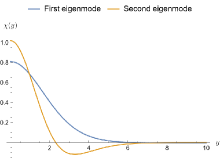
Figure 2: Graphs of the numerically determined eigenfunctions associated to the two lowest modes, assuming $y_{\rm UV}=10$.

The masses scale approximately linearly with the mode number. The right plot in figure 3 shows this behaviour for the first few mode numbers for fixed $y_{\rm UV}$. Remarkably, for large values $y_{\rm UV}>y^{*}_{\rm UV}$ the masses become independent of the UV-cutoff. This is reflecting that the eigenfunctions are localized near small $y$ so that the eigenvalues reach an asymptotic value beyond $y^{*}_{\rm UV}\approx 10$. In the left-hand side of figure 3 we display this behaviour for the first eigenmode.

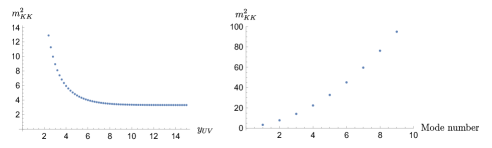
Figure 3: Left: KK mass squared of the first eigenmode as a function of $y_{\rm UV}$. Right: KK mass squared of the nine lowest eigenmodes, assuming $y_{\rm UV}=10$.

To summarize, we obtain the following scaling of the red-shifted KK masses

$$m_{{\rm KK,n}}^{2}\sim\frac{(\mathcal{V}_{w}\absolutevalue{Z}^{2})^{\frac{1}{3}}}{g_{s}^{\frac{3}{2}}M^{2}}{\rm n}^{2}M_{\rm s}^{2}\sim\frac{1}{g_{s}M^{2}}\left(\frac{\absolutevalue{Z}}{\mathcal{V}_{w}}\right)^{\frac{2}{3}}{\rm n}^{2}M_{\rm pl}^{2}\,.$$ (3.25)

Comparison with the mass of the $Z$-modulus from the previous subsection yields

$$\frac{m_{\rm KK,n}}{m_{Z}}=c\,{\rm n}$$ (3.26)

where in the regime $y_{\rm UV}<y^{*}_{\rm UV}$ the coefficient $c$ also contains a factor $y_{\rm UV}^{-1}$, which we are not explicitly writing in the following. The vast majority of KK-modes is therefore expected to be heavier than the conifold modulus. Thus, the KK-modes are parametrically of the same mass as the conifold modulus $Z$ and the description in terms of the effective action is at its limit.

As shown in [37], the existence and mass scale of these red-shifted KK-modes is consistent with the picture of emergence of the field space metric [47, 48, 49, 50], which means that integrating them out the field space metric should get a one-loop correction proportional to the tree-level result. Assuming a one-dimensional tower of red-shifted KK modes, the one-loop correction came out as

$$g_{Z\overline{Z}}^{\rm 1-loop}\sim N_{\rm sp}^{3}\frac{1}{g_{s}M^{2}}\frac{1}{\left(\mathcal{V}_{w}|Z|^{2}\right)^{2/3}}\,,$$ (3.27)

so that matching this with the tree-level metric resulting from (3.4) fixed the number $N_{\rm sp}$ of light species as

$$N_{\rm sp}\sim\left(g_{s}M^{2}\right)^{2/3}\,.$$ (3.28)

Using this scaling, we found that the one-loop corrections $g_{I\overline{J}}^{\rm 1-loop}$ of the field space metric, where $I,J\in\{Z,S,T\}$, are proportional to the tree-level expressions of the field space metric coming from the Kähler potential $K\sim M^{2}|Z|^{\frac{2}{3}}/(S+\overline{S})(T+\overline{T})$.

From the spacing and number of modes below the cutoff, one could derive for the UV cut-off

$$\begin{split}\Lambda\sim\sqrt{g_{s}M^{2}}\left({|Z|\over{\cal V}_{w}}\right)^{\!{1\over 3}}M_{\rm pl}\,\end{split}$$ (3.29)

which intriguingly equals the mass of a D3-brane wrapping the A-cycle $S^{3}$ which vanishes at the conifold singularity. Then, for the generalized species scale we get

$$\begin{split}\tilde{\Lambda}_{\text{sp}}={\Lambda\over\sqrt{N_{\rm sp}}}\sim{\Lambda\over\left(g_{s}M^{2}\right)^{1/3}}\,.\end{split}$$ (3.30)

We can express $m_{Z}\sim\Lambda/(g_{s}M^{2})$ so that in the regime of interest, $g_{s}M^{2}\gg 1$, one has the expected hierarchy $m_{Z}<\tilde{\Lambda}_{\text{sp}}$.

In summary, up to this point we have the following hierarchy of mass scales in the warped throat

$$\begin{split}\Lambda>\tilde{\Lambda}_{\text{sp}}>m_{Z}\sim m_{\rm KK}\,.\end{split}$$ (3.31)

How the mass scales of the light $S$ modulus (3.18) and the Kähler modulus fit into this hierarchy will be discussed in the next section. The bulk masses $M_{\rm cs}<M_{\rm KK}<M_{\rm s}$ are assumed to be much heavier.

4 Kähler modulus

Now, let us consider the second step of KKLT and, after integrating out $Z$ and $S$, consider the effective superpotential

$$\begin{split}W_{T}=W_{0}+A\exp(-aT)\end{split}$$ (4.1)

where $W_{0}$ is the exponentially small value from the previous race-track model for the $S$ modulus. The parameter $A$ is the so-called 1-loop Pfaffian, considered to be independent of the complex structure moduli. The parameter $a$ is defined as

$$\begin{split}a={2\pi\over N_{c}}\gamma\end{split}$$ (4.2)

where $N_{c}$ is the rank of the gauge theory featuring gaugino condensation and $\gamma$ is related to the size of the bulk 4-cycle $\tau_{\rm np}=\gamma\tau$ supporting this gauge theory. Note that for an isotropic bulk Calabi-Yau manifold one expects $\gamma=O(1)$ and that an anisotropic CY requires $h_{11}>1$.

One comment might be in order here. While this work was in preparation, employing holography, the authors of [51] suggested that no supersymmetric AdS minimum à la KKLT can possibly exist in a controlled manner. In particular, they argue that the AdS energy scale is larger than the (bulk) species scale, leading at best to a non-scale-separated AdS minimum. In addition, for the DKMM construction of perturbatively flat flux vacua, the authors argue that no supersymmetric AdS minimum can potentially exist after fixing the Kähler moduli. They say that suitable corrections to the superpotential depending on the Kähler moduli will not materialize. This means that string consistency conditions, like absence of Freed-Witten anomalies, correct number of instanton 0-modes etc., could generically forbid any such instanton correction. Here we proceed under the usual assumption that such an instanton exists and derive its consequences. This will eventually lead us to the conclusion that the uplifted de Sitter minimum of the DKMM-refined KKLT scenario is in the swampland. Thus, logically our result is consistent with [51].

4.1 Mass scales

The position $\tau$ of the supersymmetric AdS minimum is determined by the solution of the equation

$$\begin{split}\absolutevalue{A}(2a\tau+3)=3|W_{0}|e^{a\tau}\end{split}$$ (4.3)

yielding the value of the cosmological constant

$$\begin{split}V_{\rm AdS}\sim-{g_{s}\over\tau^{3}}|W_{0}|^{2}\,M_{\rm pl}^{4}\,.\end{split}$$ (4.4)

For a successful uplift to a dS vacuum, this has to be of the same scale as the $\overline{D3}$-brane tension

$$\begin{split}V_{\rm up}\sim{1\over g_{s}M^{2}}\left({|Z|\over{\cal V}_{w}}\right)^{\!{4\over 3}}\,M_{\rm pl}^{4}\,.\end{split}$$ (4.5)

This leads to

$$\begin{split}|W_{0}|\sim{1\over g_{s}|M|}\tau^{1\over 2}|Z|^{2\over 3}\,.\end{split}$$ (4.6)

We note that for an exponentially small value of $Z$, this seems to be parametrically compatible with the race-track condition ${|W_{0}|>g_{s}M^{2}|Z|/\left(\left(2\pi\right)^{2}|K|\right)}$. Indeed, combining the latter with (4.6) leads to

$$\begin{split}\left({|Z|\over{\cal V}_{w}}\right)^{1\over 3}\lesssim{\left(2\pi\right)^{2}N\over(g_{s}M^{2})^{2}}\,,\end{split}$$ (4.7)

which, however, is parametrically saturated in Scenario 1. In this case, the exponentially small $|Z|$ has to be parametrically equal to a polynomially small parameter. This might appear fairly unnatural and certainly requires a large value of the control parameter $g_{s}M^{2}$. We will see that it implies severe problems with the validity of the employed low energy effective action in the warped throat.

Moreover, we notice that the bound (4.7) is compatible with control over the warped effective action, i.e. with the upper bound (3.5) if

$$\begin{split}N\lesssim{1\over(2\pi)^{2}}\left(g_{s}M^{2}\right)^{3\over 2}\,.\end{split}$$ (4.8)

Let us proceed with the determination of the remaining parameters. For an exponentially small value of $Z$, one can estimate the value of $\tau$ as

$$\begin{split}a\tau\sim-\log|W_{0}|\lesssim-\log|Z|\sim{2\pi N\over g_{s}M^{2}}\,.\end{split}$$ (4.9)

Invoking the condition (2.20), namely $\tau>2\pi N$, one gets in both Scenario 1 and Scenario 2

$$\begin{split}\boxed{a\lesssim{1\over g_{s}M^{2}}\ll 1}\end{split}$$ (4.10)

which, as already observed in [19], is violated for an isotropic CY and a D3-brane instanton, i.e. $N_{c}=1$. The condition (4.10) must also hold in order to avoid the singular-bulk problem discussed in [23]. We notice that the string frame volume of the 4-cycle is given by $\hat{\tau}\gtrsim g_{s}N=(g_{s}|M|)|K|>1$ and therefore guaranteed to be in the large volume regime.

The mass of the Kähler modulus scales as

$$\begin{split}m_{T}\sim a{g_{s}^{1\over 2}\over{\cal V}_{w}^{1\over 3}}|W_{0}|\,M_{\rm pl}\end{split}$$ (4.11)

which, as already mentioned, scales in the same way with $|W_{0}|$ as the mass of the light $S$ modulus. Therefore, one might suspect that first integrating out $S$ is not self-consistent. It was argued in [30, 31] that as long as the parameter $A$ in the KKLT superpotential does not depend on any complex structure modulus, the minimum prevails. We checked this numerically in concrete examples.

4.2 Mass hierarchies extended

Now we would like to see how the mass scale of the uplift potential fits into the hierarchies of scales in (3.31). Using (4.5) we can write

$$\begin{split}V_{\rm up}^{1\over 4}\sim{\Lambda\over(g_{s}M^{2})^{3\over 4}}\,\end{split}$$ (4.12)

which is smaller than the species scale and larger than the mass of $Z$.

Next we analyze the relation between the mass of the Kähler modulus and the light KK scale. Using the relations (4.6) and (4.9) one gets

$$\begin{split}{m_{T}}\lesssim{2\pi N\over(g_{s}M^{2})^{3\over 2}}\left({|Z|\over{\cal V}_{w}}\right)^{\!{2\over 3}}M_{\rm pl}\sim{2\pi N\over(g_{s}M^{2})^{2}}\left({|Z|\over{\cal V}_{w}}\right)^{\!{1\over 3}}\,\Lambda\,.\end{split}$$ (4.13)

Thus, one finds

$$\begin{split}{m_{T}\over m_{\rm KK}}\lesssim{2\pi N\over(g_{s}M^{2})}\left({|Z|\over{\cal V}_{w}}\right)^{\!{1\over 3}}\lesssim{\left(2\pi\right)^{3}N^{2}\over(g_{s}M^{2})^{3}}\lesssim 1\,,\end{split}$$ (4.14)

where we have used the relation (4.7) in the second step and the constraint (4.8) needed for the control of the effective theory in the last step. Hence, we have the desired hierarchy $m_{T}<m_{\rm KK}$.

Let us perform a similar analysis for the relation between the mass of the $S$ modulus and the light KK scale. Using the relation (4.6) one gets for Scenario 2

$$\begin{split}{m^{(2)}_{S}\over m_{\rm KK}}\sim{c_{1}c_{2}\over g_{s}^{2}}\left({|Z|\over{\cal V}_{w}}\right)^{\!{1\over 3}}\lesssim{\left(2\pi\right)^{2}c_{1}c_{2}N\over(g_{s}M)^{4}}\,,\end{split}$$ (4.15)

where we have used the relation (4.7) in the last step. Hence a sufficient condition for having the desired hierarchy $m^{(2)}_{S}<m_{\rm KK}\sim m_{Z}$ is

$$\begin{split}\boxed{\left(2\pi\right)^{2}c_{1}c_{2}N<(g_{s}M)^{4}}\,.\end{split}$$ (4.16)

As already mentioned in section 3.1, we find in Scenario 1 the ratio

$${m^{(1)}_{S}\over m_{Z}}={N\over\tau}|Z|^{2\over 3}\ll 1\,,$$ (4.17)

where we have used that $\tau>N$. Hence, we have the desired hierarchy $m^{(1)}_{S}<m_{\rm KK}\sim m_{Z}$ in Scenario 1. Note that in Scenario 1, for the ratio of the two lightest moduli we find

$$\begin{split}{m_{T}\over m^{(1)}_{S}}\sim{g_{s}M^{2}\over 2\pi N}\lesssim 1\,,\end{split}$$ (4.18)

where the inequality in the second step has to hold to guarantee $|Z|\ll 1$.

Summarizing, our analytic analysis revealed the following order of all the relevant red-shifted mass scales of the warped throat

$$\Lambda>\tilde{\Lambda}_{\text{sp}}>V^{1\over 4}_{\text{up}}>m_{Z}\sim m_{\rm KK}>m_{S/T}\,,$$ (4.19)

where we have the hierarchy $m^{(1)}_{S}>m_{T}$ in Scenario 1 and there is no definite hierarchy between the masses $m^{(2)}_{S}$ and $m_{T}$ in Scenario 2.

Mass scales in Scenario 1

Let us first consider the mass scales in Scenario 1 in more detail. Upon invoking the parametrically saturated relation (4.7), the cut-off can be expressed as

$$\begin{split}\Lambda\sim{\left(2\pi\right)^{2}N\over(g_{s}M^{2})^{3\over 2}}M_{\text{pl}}\,.\end{split}$$ (4.20)

We have seen that the masses in the throat are ordered in the expected manner. However, using the saturated relation (4.7), one can now express the lightest bulk mass scale (3.2) as

$$\begin{split}M_{\rm cs}\sim g_{s}^{1\over 2}{(g_{s}M^{2})^{3\over 2}\over\left(2\pi\right)^{2}N\tau^{3\over 2}}\Lambda\lesssim{g_{s}^{1\over 2}\over 2\pi}{\left(g_{s}M^{2}\right)^{3\over 2}\over\left(2\pi N\right)^{5\over 2}}\Lambda\,\end{split}$$ (4.21)

which implies

$$\begin{split}M_{\rm cs}\lesssim{g_{s}^{1\over 2}\over 2\pi}\left({g_{s}M^{2}\over 2\pi N}\right)^{5\over 2}m_{\rm KK}\lesssim m_{\rm KK}\,.\end{split}$$ (4.22)

This means that the bulk complex structure moduli are lighter than the red-shifted KK-modes in the throat. Hence, in Scenario 1 the bulk and throat are not energetically separated, spoiling completely the validity of the used effective action in the throat. One might think that this is to be expected from the very begining as we were balancing a term in the IR (throat) against a term in the UV (bulk). However, notice that the tree-level UV term is vanishing by construction and that in the racetrack potential (3.11) we were balancing the IR energy against a non-perturbative bulk term. That this spoils decoupling of bulk and throat is not obvious.

Next we analyze the relation between the lightest bulk mass scale $M_{\rm cs}$ and the mass of the $S$ modulus. Using the saturated relation (4.7), we get the ratio

$$\begin{split}{M_{\rm cs}\over m_{S}^{(1)}}\sim{g_{s}^{1\over 2}\over\tau^{3\over 2}}\,{\left(g_{s}M^{2}\right)^{13\over 2}\over\left(2\pi\right)^{6}N^{4}}\,\end{split}$$ (4.23)

so that imposing $M_{\rm cs}>m_{S}^{(1)}$ sets an upper bound on $\tau$.

Let us roughly estimate the number of bulk complex structure moduli to be ${h_{31}\sim\chi(Y)\gtrsim N}$, where in the final step we have assumed that the large tadpole from the fluxes in the throat $N=MK$ is not cancelled by other contributions. Since these extra fields and all their KK-modes are now light, the species scale also becomes smaller and can be estimated as

$$\begin{split}\tilde{\Lambda}_{\text{sp}}\lesssim{\Lambda\over N^{1\over 2}(g_{s}M^{2})^{1\over 3}}\,.\end{split}$$ (4.24)

Apparently, this scale is smaller than $V_{\rm up}^{1\over 4}$ as

$$\begin{split}\tilde{\Lambda}_{\text{sp}}\lesssim\left({g_{s}M^{2}\over N}\right)^{1\over 2}V_{\rm up}^{1\over 4}\lesssim V_{\rm up}^{1\over 4}\,.\end{split}$$ (4.25)

We notice that for this more specific model we have arrived at a very similar conclusion as [51], though not using holography but the existence of an uplift of the initial AdS-minimum. In table 1 we show the hierarchy of the bulk and the throat mass scales. On the left we list the expected order, if there were a separation between the bulk and the red-shifted throat. On the right, we list the non-separated mass scales found for Scenario 1.

bulk-throat separated scales
$M_{\rm cs}\sim{\sqrt{g_{s}}\over{\cal V}_{w}}M_{\rm pl}$
$\Lambda\sim M_{\text{pl}}\eta^{3\over 2}N$
$\tilde{\Lambda}_{\text{sp}}\sim\eta^{\frac{1}{3}}\Lambda$
$V_{\rm up}^{1\over 4}\sim\eta^{\frac{3}{4}}\Lambda$
$m_{Z}\sim m_{\rm KK}\sim\eta\Lambda$
$m_{S}^{(1)}\sim N^{3}\,\eta^{5}\Lambda$
$m_{T}\sim N^{2}\,\eta^{4}\Lambda$

bulk-throat mixed scales
$\Lambda\sim M_{\text{pl}}\eta^{3\over 2}N$
$V_{\rm up}^{1\over 4}\sim\eta^{\frac{3}{4}}\Lambda$
$\tilde{\Lambda}_{\text{sp}}\lesssim N^{-{1\over 2}}\eta^{\frac{1}{3}}\Lambda$
$m_{Z}\sim m_{\rm KK}\sim\eta\Lambda$
$M_{\rm cs}\lesssim g_{s}^{1\over 2}N^{-{5\over 2}}\eta^{-{3\over 2}}\Lambda$
$m_{S}^{(1)}\sim N^{3}\,\eta^{5}\Lambda$
$m_{T}\sim N^{2}\,\eta^{4}\Lambda$

Table 1: Expected separated and realistic mixed mass scales for Scenario 1. We have defined the parameter $\eta=1/\left(g_{s}M^{2}\right)$.

In addition, we have a very large tadpole contribution from the fluxes. From the now saturated relation (4.7), we can derive the lower bound

$$\begin{split}N\gtrsim 2\pi(\log|Z|)^{4}|Z|^{-{2\over 3}}\,,\end{split}$$ (4.26)

where we also used (2.20). Remarkably, the bound is solely determined by the VEV of the conifold modulus. To get a better impression, let us assume that for having control over the geometry and the effective action we need the conifold modulus in a regime $|Z|<10^{-5}$. Then equation (4.26) tells us that $N>10^{8}$, which implies $M\sim 10^{4}$ and $a<10^{-7}$ (for $M\approx N^{1\over 2}$ and $g_{s}\sim 0.1$). For $|Z|<10^{-4}$ one finds $N>10^{7}$.

Thus, in addition to having the wrong hierarchy we face large integers, i.e. large fluxes and numbers of branes, large tadpole contributions and either large non-isotropies in the bulk or a high rank confining gauge group.

Mass scales in Scenario 2

This case is less constrained, as we treat the parameters $c_{1}$ and $c_{2}$ in the race-track potential as free parameters. Thus the constraint (4.7) is mild now. Indeed, the lightest bulk mass scale $M_{\rm cs}$ is larger than the cut-off $\Lambda$, if

$$\begin{split}\left({\cal V}_{w}^{2}|Z|\right)^{1/3}\lesssim\frac{1}{|M|}\,.\end{split}$$ (4.27)

In this case the bulk and the throat are energetically decoupled and we have the following hierarchies of scales

$$M_{\rm cs}>\Lambda>\tilde{\Lambda}_{\text{sp}}>V^{1\over 4}_{\text{up}}>m_{Z}\sim m_{\rm KK}>m_{S/T}\,.$$ (4.28)

As a proof of principle, in the next section we provide an example that features the intended hierarchy (4.28) of all masses.

However, we can still derive a lower bound on the fluxes in the throat. From the uplift condition (4.6) and the relations (3.13) and (3.10) it follows that

$$\begin{split}{|c_{2}-c_{1}|\over c_{2}}\,|a_{1}|\,e^{-c_{1}s_{0}}\sim{1\over g_{s}|M|}\tau^{1\over 2}|\zeta_{0}|^{2\over 3}e^{-{2\over 3}{2\pi K\over M}s_{0}}\,.\end{split}$$ (4.29)

Setting the exponentially small terms in (4.29) to be of the same scale, we can estimate

$$\begin{split}c_{1}\sim{4\pi K\over 3M}\,.\end{split}$$ (4.30)

Invoking now the (slightly concretized) bound $g_{s}|M|\gtrsim O(10^{n})$ from (2.12), set by having a valid supergravity, large radius description, we get

$$\begin{split}M\gtrsim{10^{n}\over g_{s}}\,,\qquad K\gtrsim{10^{n}c_{1}\over g_{s}}\,,\qquad N\gtrsim{10^{2n}c_{1}\over g_{s}^{2}}\,.\end{split}$$ (4.31)

Assuming $c_{1}>g_{s}$ for a controlled race-track minimum, $g_{s}\lesssim 0.1$ for control over string loop corrections and $g_{s}|M|\gtrsim 10$ for a controlled supergravity description, one finds $N\gtrsim 10^{2-3}$. This is still a moderately large contribution that might be in conflict with tadpole cancellation or the tadpole conjecture, respectively. For fully fledged models we expect the bound to be much more stringent, as we treated the race-track parameters as free parameters while for concrete Calabi-Yau manifolds they are also determined by three-form fluxes contributing to the tadpole themselves. Hence, the tadpole will easily exceed the above simple estimate by orders of magnitude.

Comments on tadpole cancellation

Recall that the tadpole cancellation condition reads

$$\begin{split}MK+N_{\rm flux}+N_{\rm brane}={\chi(Y)\over 24}\end{split}$$ (4.32)

where $N_{\rm flux}$ denotes the contribution of the other present fluxes and $N_{\rm brane}$ the contribution from D3-branes and magnetized D7-branes. For such a large flux $N=MK$ one does not expect (almost fine tuned) cancellations between the various flux and brane contributions to occur. Therefore, one needs a Calabi-Yau fourfold with a very large Euler characteristic $\chi(Y)$. This will have many complex structure moduli so that one very likely encounters the problem of the tadpole conjecture [42, 43, 44, 45]. Namely, that it is not possible to freeze all of these many moduli using three-form fluxes, something that was silently assumed before we focused just on the final two moduli $Z$ and $S$. Hence, we arrive at the conclusion that a working DKMM-refined KKLT Scenario 1 would require very large fluxes that are in conflict with the tadpole constraint. Scenario 2 is expected to be much more constrained in concrete cases, so that the flux tadpole could become dangerously large, likewise. Note that a very similar conclusion was drawn recently for a controlled Large Volume Scenario [52, 53, 54].

5 Numerical analysis

Since throughout our analysis we were invoking quite a number of approximations, we need to provide a proof of principle. For this purpose, let us now test the previous results by comparing them with concrete numerical solutions of the problem.

We consider the full scalar potential after analytically stabilizing the conifold modulus and systematically search for a region in parameter space with a dS minimum by making use of the uplift condition, which will be written as

$$\begin{split}\kappa{g_{s}|W_{0}|^{2}\over\tau_{0}^{3}}\sim{\xi\over g_{s}M^{2}}{|Z|^{4\over 3}\over\tau_{0}^{2}}\end{split}$$ (5.1)

where $\xi$ is the numerical prefactor appearing in the uplift potential and we introduced an order one “balance” parameter $\kappa$. Since order one factors do matter in this analysis, we have at least taken factors of $(2\pi)$ into account. In hindsight, utilizing results from moduli stabilization we derive a condition on the fluxes $(M,K,M_{1})$ for a successful uplift.

The construction of a working uplift turns out to be quite challenging if the free race-track parameters are all dialed by hand. Thus, we make specific assumptions for some coefficients to simplify our search. Recall that after the stabilization of the conifold modulus, the generic superpotential reads

$$\begin{split}W=a_{1}e^{-c_{1}S}+a_{2}e^{-c_{2}S}\end{split}$$ (5.2)

and its value at the minimum can be approximated by

$$\begin{split}W_{0}\sim{c_{2}-c_{1}\over c_{2}}a_{1}e^{-c_{1}S_{0}}\end{split}$$ (5.3)

with $S_{0}$ given by (3.12) as usual. Motivated by the race-track scenario with non-perturbative terms generated via gaugino condensation, we now assume $c_{i}<1$ and that the second exponent in the superpotential is given in terms of the first one via

$$\begin{split}c_{2}=(c_{1}^{-1}-1)^{-1}\,.\end{split}$$ (5.4)

The factor $a_{2}$ can be adjusted such that the log-term in (3.12) is a number of order one. With these premises we derive the following expressions for $W_{0}$ and the string coupling $g_{s}$:

$$\begin{split}W_{0}\sim a_{1}c_{1}\exp\left(-\frac{1}{c_{1}}\right)\,,\qquad g_{s}\sim c_{1}^{2}\,.\end{split}$$ (5.5)

Thus, this ansatz guarantees that we have control over the race-track potential as $g_{s}\sim c_{1}^{2}<c_{1}$ for $c_{1}<1$.

Moreover, $W_{0}$ allows us to estimate the value of $\tau$ via (4.9). To improve the quality of our estimate the log-log correction will be taken into account, meaning that

$$\begin{split}a\tau\sim\log{\absolutevalue{W_{0}}^{-1}}+\log{\log{\absolutevalue{W_{0}}^{-1}}}.\end{split}$$ (5.6)

This effectively increases our estimate for $a\tau$ in both scenarios. Respecting the condition $\tau>2\pi N$, we can express it as

$$\begin{split}a={\lambda\over 2\pi N}\left(\log{\absolutevalue{W_{0}}^{-1}}+\log{\log{\absolutevalue{W_{0}}^{-1}}}\right)\end{split}$$ (5.7)

where we introduced a factor $0<\lambda<1$, which for each concrete numerical example allows some tuning. The Pfaffian $A$ is taken to be $-1$ and the coefficient $\xi$ is taken to be $\frac{63}{32}$ in all concrete realizations presented below. For later purposes, we define the two parameters

$$\begin{split}X={M\over 2\pi K}\,,\qquad\quad Y=2\pi|K|\,.\end{split}$$ (5.8)

5.1 Scenario 1

In Scenario 1 we have $a_{1}=M\zeta_{0}/(2\pi)$ and $c_{1}=2\pi K/M$, so the conifold modulus and the superpotential are given by

$$\begin{split}Z\sim\zeta_{0}\exp\left(-{M\over 2\pi K}\right)\,,\qquad W_{0}\sim K\zeta_{0}\exp\left(-{M\over 2\pi K}\right)\end{split}$$ (5.9)

and the uplift condition (5.1) can be expressed as

$$\begin{split}{\xi\over\kappa}{2\pi\over Y^{2}}X^{3}\left|\zeta_{0}\right|^{-2/3}\exp\left({2X\over 3}\right)\simeq\lambda\,.\end{split}$$ (5.10)

For really finding parameters allowing a controllable dS uplift, this condition needs to be satisfied with a sufficient accuracy. Let us stress that (5.7) leads to the following refinement of the condition (4.10)

$$\begin{split}a\lesssim{2\pi\over g_{s}M^{2}}+\frac{1}{N}\log\left({2\pi\over g_{s}|M|\left|\zeta_{0}\right|}\right)\ll 1\,.\end{split}$$ (5.11)

As a consequence, the search for a numerical realization becomes a lot easier.

Employing the above recipe, we were able to construct numerical realizations with a tadpole of $O(10^{19})$ induced by the throat fluxes, which surpasses the expected lower bound (4.26) by many orders of magnitude. These examples also confirm the unphysical mass hierarchy with mixed throat and bulk scales. Our large flux numbers are especially enforced by the stabilized $\tau$-modulus. Indeed, the smallness of the $a$ coefficient and the uplift condition impose such a large value for $\tau$, as the strong warping condition (2.4) turns out to be violated below $N\sim O(10^{19})$. It may be possible to get closer to the theoretical lower bound of $N\sim 10^{7-8}$ in more finely tuned setups, but in any case the flux tadpole of Scenario 1 has certainly almost no chance to be cancelled in realistic situations.

5.2 Scenario 2

In the second scenario, the race-track coefficients are not determined by the flux numbers $M,K,M_{1}$ and we dial them freely as long as we stay in the controlled regime. However, keep in mind that in concrete realizations those coefficients are not free parameters but also set by other flux numbers and data of the underlying Calabi-Yau manifold. Therefore, the way we proceed is very optimistic and eventually Scenario 2 will also be much more constrained. Setting $a_{1}=1$ for convenience, we can derive the following uplift constraint for Scenario 2:

$$\begin{split}{\xi\over\kappa}(2\pi X)^{-1}c_{1}^{-6}|\zeta_{0}|^{\frac{4}{3}}\exp\left({2\over c_{1}}-\frac{4}{3}\frac{1}{c_{1}^{2}X}\right)\simeq\lambda\,.\end{split}$$ (5.12)

One numerical example is specified by $c_{1}=1/40$, $\lambda=9/10$, $\kappa=1/2$, $M=5\,000$, ${K=37}$ and $M_{1}=\frac{M}{2\pi i}$. The coefficient $a$ is therefore $a\approx 3.67\cdot 10^{-5}$. The D3-brane tadpole contribution is of order ${N=O(10^{5})}$, which is smaller than in Scenario 1 but still fairly large. For $s\rvert_{\text{num}}\approx 1\,599.75$ and $\tau\rvert_{\text{num}}\approx 1.30\cdot 10^{6}$ the dS minimum is found at

$$\begin{split}V_{0}\rvert_{\text{num}}\approx 5.88\cdot 10^{-60}M_{\text{pl}}^{4}\,.\end{split}$$ (5.13)

In table 2 we show the numerical values of the mass scales in the left-hand column. The numerical values of the mass scale of the bulk complex structure moduli and the scales $\Lambda$ and $\tilde{\Lambda}_{\text{sp}}$ were determined via the relations (3.2), (3.29) and (3.30) respectively. $V_{\rm up}^{1\over 4}$ and the mass scale $m_{\rm KK}$ were obtained via (3.20) and (3.25) respectively. The masses of the lightest saxions $s$ and $\tau$ were obtained via (3.16).

numerical values	theoretical predictions
$M_{\rm cs}\approx 1.69\cdot 10^{-11}M_{\text{pl}}$	$M_{\rm cs}\approx 1.71\cdot 10^{-11}M_{\text{pl}}$
$\Lambda\approx 1.87\cdot 10^{-12}{M_{\rm pl}}$	$\Lambda\approx 1.87\cdot 10^{-12}{M_{\rm pl}}$
$\tilde{\Lambda}_{\text{sp}}\approx 7.50\cdot 10^{-14}M_{\text{pl}}$	$\tilde{\Lambda}_{\text{sp}}\approx 7.50\cdot 10^{-14}M_{\text{pl}}$
$V_{\rm up}^{1\over 4}\approx 1.59\cdot 10^{-15}M_{\text{pl}}$	$V_{\rm up}^{1\over 4}\approx 1.59\cdot 10^{-15}M_{\text{pl}}$
$m_{Z}\sim m_{\rm KK}\approx 1.20\cdot 10^{-16}M_{\text{pl}}$	$m_{Z}\sim m_{\rm KK}\approx 1.20\cdot 10^{-16}M_{\text{pl}}$
$m_{s}\approx 3.00\cdot 10^{-27}M_{\text{pl}}$	$m_{s}\approx 2.99\cdot 10^{-27}M_{\text{pl}}$
$m_{\tau}\approx 2.10\cdot 10^{-29}M_{\text{pl}}$	$m_{\tau}\approx 8.59\cdot 10^{-29}M_{\text{pl}}$

Table 2: The numerical values and the theoretical predictions of the mass scales for Scenario 2.

This has to be compared with our theoretical predictions. Here we find the dS minimum at $s\rvert_{\text{theo}}\approx 1\,600.00$ and $\tau\rvert_{\text{theo}}\approx 1.29\cdot 10^{6}$ with the value of the potential being

$$\begin{split}V_{0}\rvert_{\text{theo}}\approx 5.98\cdot 10^{-60}M_{\text{pl}}^{4}\,.\end{split}$$ (5.14)

In the right-hand column of table 2, we list the theoretical predictions of the mass scales, using the same formulas as those used for the numerical values, except for the masses of the lightest saxions, whose theoretical values were obtained with the approximate formulas (3.18) and (4.11).

Hence, the theoretical predictions for the mass scales are in agreement with the numerical results. Again we show plots of the potential close to this minimum in the figures 4 and 5.

Figure 4: Plots of scalar potential showing a realization of Scenario 2. Left: $V(s,\tau)$ for $\tau\approx 1.30\cdot 10^{6}$ and right: $V(s,\tau)$ for $s\approx 1\,599.75$, both multiplied by $10^{60}$. Choice of parameters: $c_{1}=1/40$, $\lambda=9/10$, $\kappa=1/2$, $M=5\,000$, $K=37$, $M_{1}=\frac{M}{2\pi i}$.

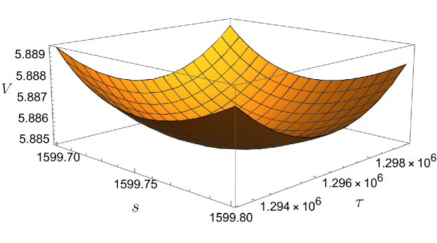
Figure 5: Potential $V(s,\tau)$ for our example from Scenario 2, multiplied by $10^{60}$. Choice of parameters: $c_{1}=1/40$, $\lambda=9/10$, $\kappa=1/2$, $M=5\,000$, $K=37$, $M_{1}=\frac{M}{2\pi i}$.

This example for Scenario 2 indicates that while the hierarchy of mass scales is in order, the fluxes $M,K$ needed to stabilize the conifold modulus and the axio-dilaton yield a moderately large contribution $N=MK$ to the D3-brane tadpole. By choosing different values for the parameters one might come even closer to the general bound $N>10^{3-4}$.

6 Conclusion

In this paper we extended the usual KKLT construction by the concrete mechanism of DKMM to stabilize the complex structure moduli such that $W_{0}$ is guaranteed to be exponentially small. The objective was to derive what additional constraints this imposes on the length and mass scales of the geometry and the light fields involved.

First, using geometric consistency constraints we derived a lower and an upper bound for the length of the throat. Mutual consistency then directly led us to a bound for the four-cycle volume in terms of the D3-tadpole contribution coming from the throat fluxes. Thus, this direct computation for the Klebanov-Strassler throat is consistent with a former indirect argument using the D3-brane backreaction [19].

We then considered the explicit stabilization of the final light moduli $(Z,S,T)$, working in a framework where all heavier complex structure moduli have been assumed to be fixed via three-form fluxes. We employed the methods and the analysis of [37], but generalized it such that we also included the axio-dilaton and therefore the string coupling constant in the set of light fields. Following the generalization of the DKMM mechanism to the conifold regime we invoked a race-track scenario for its stabilization. For the absence of non-perturbative corrections in the Kähler moduli, the scalar potential was found to be positive-semidefinite and to obey a modified no-scale structure.

Computing the appearing mass scales, we found that this DKMM-refined KKLT scenario comes with a couple of strong constraints. In our more restricted Scenario 1 we found that one is driven to a regime where the bulk mass scale does not decouple from the throat mass scale. Clearly, this invalidates the employed low energy effective action in the throat. Moreover, analogous to the recent work [51] we found that as a consequence, the energy scale of the uplift is parametrically larger than the (throat) species scale. Recall that [51] claim that the whole DKMM construction ceases to be controllable even before the uplift.

We also found that for both Scenario 1 and Scenario 2, the two flux quanta $M,K$ need to be fairly large, in fact much larger than what was derived from the non-destabilization of the conifold modulus in [36]. Moreover, also the parameter $a$ that appears in the combination $aT$ in the non-perturbative term needs to be extremely small, which requires either a high rank confining gauge group or a highly non-isotropic 4-cycle. All this was confirmed by concrete numerical examples, whose throat mass scales were consistent with our theoretical predictions. In view of the recent tadpole conjecture, this raises some additional doubts that the DKMM-refined KKLT scenario is in the landscape of string theory.

Acknowledgments

We would like to thank Andriana Makridou and Erik Plauschinn for helpful discussions. We are also grateful to Arthur Hebecker, Daniel Junghans and Severin Lüst for clarifying comments about a former version of this paper.

References

- [1] S. Kachru, R. Kallosh, A. D. Linde, and S. P. Trivedi, “De Sitter vacua in string theory,” Phys. Rev. D 68 (2003) 046005, hep-th/0301240.
- [2] C. Vafa, “The String landscape and the swampland,” hep-th/0509212.
- [3] H. Ooguri and C. Vafa, “On the Geometry of the String Landscape and the Swampland,” Nucl. Phys. B 766 (2007) 21–33, hep-th/0605264.
- [4] T. D. Brennan, F. Carta, and C. Vafa, “The String Landscape, the Swampland, and the Missing Corner,” PoS TASI2017 (2017) 015, 1711.00864.
- [5] E. Palti, “The Swampland: Introduction and Review,” Fortsch. Phys. 67 (2019), no. 6, 1900037, 1903.06239.
- [6] M. van Beest, J. Calderón-Infante, D. Mirfendereski, and I. Valenzuela, “Lectures on the Swampland Program in String Compactifications,” 2102.01111.
- [7] G. Obied, H. Ooguri, L. Spodyneiko, and C. Vafa, “De Sitter Space and the Swampland,” 1806.08362.
- [8] H. Ooguri, E. Palti, G. Shiu, and C. Vafa, “Distance and de Sitter Conjectures on the Swampland,” Phys. Lett. B 788 (2019) 180–184, 1810.05506.
- [9] S. K. Garg and C. Krishnan, “Bounds on Slow Roll and the de Sitter Swampland,” JHEP 11 (2019) 075, 1807.05193.
- [10] D. Andriot, “On the de Sitter swampland criterion,” Phys. Lett. B 785 (2018) 570–573, 1806.10999.
- [11] A. Bedroya and C. Vafa, “Trans-Planckian Censorship and the Swampland,” JHEP 09 (2020) 123, 1909.11063.
- [12] U. H. Danielsson and T. Van Riet, “What if string theory has no de Sitter vacua?,” Int. J. Mod. Phys. D 27 (2018), no. 12, 1830007, 1804.01120.
- [13] J. Moritz, A. Retolaza, and A. Westphal, “Toward de Sitter space from ten dimensions,” Phys. Rev. D97 (2018), no. 4, 046010, 1707.08678.
- [14] R. Kallosh, A. Linde, E. McDonough, and M. Scalisi, “de Sitter Vacua with a Nilpotent Superfield,” Fortsch. Phys. 2018 (2018) 1800068, 1808.09428.
- [15] R. Kallosh, A. Linde, E. McDonough, and M. Scalisi, “4D models of de Sitter uplift,” Phys. Rev. D99 (2019), no. 4, 046006, 1809.09018.
- [16] F. F. Gautason, V. Van Hemelryck, and T. Van Riet, “The tension between 10D supergravity and dS uplifts,” Fortsch. Phys. 67 (2019), no. 1-2, 1800091, 1810.08518.
- [17] Y. Hamada, A. Hebecker, G. Shiu, and P. Soler, “On brane gaugino condensates in 10d,” JHEP 04 (2019) 008, 1812.06097.
- [18] Y. Hamada, A. Hebecker, G. Shiu, and P. Soler, “Understanding KKLT from a 10d perspective,” JHEP 06 (2019) 019, 1902.01410.
- [19] F. Carta, J. Moritz, and A. Westphal, “Gaugino condensation and small uplifts in KKLT,” JHEP 08 (2019) 141, 1902.01412.
- [20] F. F. Gautason, V. Van Hemelryck, T. Van Riet, and G. Venken, “A 10d view on the KKLT AdS vacuum and uplifting,” JHEP 06 (2020) 074, 1902.01415.
- [21] I. Bena, M. Graña, N. Kovensky, and A. Retolaza, “Kähler moduli stabilization from ten dimensions,” JHEP 10 (2019) 200, 1908.01785.
- [22] R. Blumenhagen, M. Brinkmann, D. Kläwer, A. Makridou, and L. Schlechter, “KKLT and the Swampland Conjectures,” PoS CORFU2019 (2020) 158, 2004.09285.
- [23] X. Gao, A. Hebecker, and D. Junghans, “Control issues of KKLT,” Fortsch. Phys. 68 (2020) 2000089, 2009.03914.
- [24] M. Demirtas, M. Kim, L. Mcallister, and J. Moritz, “Vacua with Small Flux Superpotential,” Phys. Rev. Lett. 124 (2020), no. 21, 211603, 1912.10047.
- [25] M. Demirtas, M. Kim, L. McAllister, and J. Moritz, “Conifold Vacua with Small Flux Superpotential,” Fortsch. Phys. 68 (2020) 2000085, 2009.03312.
- [26] R. Álvarez-García, R. Blumenhagen, M. Brinkmann, and L. Schlechter, “Small Flux Superpotentials for Type IIB Flux Vacua Close to a Conifold,” Fortsch. Phys. 68 (2020) 2000088, 2009.03325.
- [27] R. Álvarez-García and L. Schlechter, “Analytic Periods via Twisted Symmetric Squares,” 2110.02962.
- [28] B. Bastian, T. W. Grimm, and D. van de Heisteeg, “Engineering Small Flux Superpotentials and Mass Hierarchies,” 2108.11962.
- [29] Y. Honma and H. Otsuka, “Small flux superpotential in F-theory compactifications,” Phys. Rev. D 103 (2021), no. 12, 126022, 2103.03003.
- [30] M. Demirtas, M. Kim, L. McAllister, J. Moritz, and A. Rios-Tascon, “Small cosmological constants in string theory,” JHEP 12 (2021) 136, 2107.09064.
- [31] M. Demirtas, M. Kim, L. McAllister, J. Moritz, and A. Rios-Tascon, “Exponentially Small Cosmological Constant in String Theory,” Phys. Rev. Lett. 128 (2022), no. 1, 011602, 2107.09065.
- [32] I. Broeckel, M. Cicoli, A. Maharana, K. Singh, and K. Sinha, “On the Search for Low ,” 2108.04266.
- [33] F. Carta, A. Mininno, and P. Shukla, “Systematics of perturbatively flat flux vacua,” JHEP 02 (2022) 205, 2112.13863.
- [34] F. Carta, A. Mininno, and P. Shukla, “Systematics of perturbatively flat flux vacua for CICYs,” 2201.10581.
- [35] M. R. Douglas, J. Shelton, and G. Torroba, “Warping and supersymmetry breaking,” 0704.4001.
- [36] I. Bena, E. Dudas, M. Graña, and S. Lüst, “Uplifting Runaways,” Fortsch. Phys. 67 (2019), no. 1-2, 1800100, 1809.06861.
- [37] R. Blumenhagen, D. Kläwer, and L. Schlechter, “Swampland Variations on a Theme by KKLT,” JHEP 05 (2019) 152, 1902.07724.
- [38] I. Bena, A. Buchel, and S. Lüst, “Throat destabilization (for profit and for fun),” 1910.08094.
- [39] E. Dudas and S. Lüst, “An update on moduli stabilization with antibrane uplift,” JHEP 03 (2021) 107, 1912.09948.
- [40] L. Randall, “The Boundaries of KKLT,” Fortsch. Phys. 68 (2020), no. 3-4, 1900105, 1912.06693.
- [41] S. Lüst and L. Randall, “Effective Theory of Warped Compactifications and the Implications for KKLT,” 2206.04708.
- [42] I. Bena, J. Blåbäck, M. Graña, and S. Lüst, “The tadpole problem,” JHEP 11 (2021) 223, 2010.10519.
- [43] I. Bena, J. Blåbäck, M. Graña, and S. Lüst, “Algorithmically Solving the Tadpole Problem,” Adv. Appl. Clifford Algebras 32 (2022), no. 1, 7, 2103.03250.
- [44] E. Plauschinn, “The tadpole conjecture at large complex-structure,” JHEP 02 (2022) 206, 2109.00029.
- [45] M. Graña, T. W. Grimm, D. van de Heisteeg, A. Herraez, and E. Plauschinn, “The Tadpole Conjecture in Asymptotic Limits,” 2204.05331.
- [46] I. R. Klebanov and M. J. Strassler, “Supergravity and a confining gauge theory: Duality cascades and chi SB resolution of naked singularities,” JHEP 08 (2000) 052, hep-th/0007191.
- [47] B. Heidenreich, M. Reece, and T. Rudelius, “The Weak Gravity Conjecture and Emergence from an Ultraviolet Cutoff,” Eur. Phys. J. C78 (2018), no. 4, 337, 1712.01868.
- [48] T. W. Grimm, E. Palti, and I. Valenzuela, “Infinite Distances in Field Space and Massless Towers of States,” JHEP 08 (2018) 143, 1802.08264.
- [49] B. Heidenreich, M. Reece, and T. Rudelius, “Emergence of Weak Coupling at Large Distance in Quantum Gravity,” Phys. Rev. Lett. 121 (2018), no. 5, 051601, 1802.08698.
- [50] P. Corvilain, T. W. Grimm, and I. Valenzuela, “The Swampland Distance Conjecture for Kähler moduli,” JHEP 08 (2019) 075, 1812.07548.
- [51] S. Lüst, C. Vafa, M. Wiesner, and K. Xu, “Holography and the KKLT Scenario,” 2204.07171.
- [52] D. Junghans, “LVS de Sitter Vacua are probably in the Swampland,” 2201.03572.
- [53] X. Gao, A. Hebecker, S. Schreyer, and G. Venken, “Loops, Local Corrections and Warping in the LVS and other Type IIB Models,” 2204.06009.
- [54] D. Junghans, “Topological Constraints in the LARGE-Volume Scenario,” 2205.02856.
- [55] S. B. Giddings, S. Kachru, and J. Polchinski, “Hierarchies from fluxes in string compactifications,” Phys. Rev. D 66 (2002) 106006, hep-th/0105097.
- [56] C. P. Herzog, I. R. Klebanov, and P. Ouyang, “Remarks on the warped deformed conifold,” in Modern Trends in String Theory: 2nd Lisbon School on g Theory Superstrings. 8, 2001. hep-th/0108101.
- [57] M. R. Douglas and G. Torroba, “Kinetic terms in warped compactifications,” JHEP 05 (2009) 013, 0805.3700.
- [58] R. Kallosh and A. D. Linde, “Landscape, the scale of SUSY breaking, and inflation,” JHEP 12 (2004) 004, hep-th/0411011.
- [59] A. R. Frey and A. Maharana, “Warped spectroscopy: Localization of frozen bulk modes,” JHEP 08 (2006) 021, hep-th/0603233.
- [60] C. P. Burgess, P. G. Camara, S. P. de Alwis, S. B. Giddings, A. Maharana, F. Quevedo, and K. Suruliz, “Warped Supersymmetry Breaking,” JHEP 04 (2008) 053, hep-th/0610255.
- [61] G. Shiu, G. Torroba, B. Underwood, and M. R. Douglas, “Dynamics of Warped Flux Compactifications,” JHEP 06 (2008) 024, 0803.3068.
- [62] S. P. de Alwis, “Constraints on Dbar Uplifts,” JHEP 11 (2016) 045, 1605.06456.
- [63] G. Dvali, “Black Holes and Large N Species Solution to the Hierarchy Problem,” Fortsch. Phys. 58 (2010) 528–536, 0706.2050.
- [64] G. Dvali and M. Redi, “Black Hole Bound on the Number of Species and Quantum Gravity at LHC,” Phys. Rev. D 77 (2008) 045027, 0710.4344.