On the Fountain Effect in Superfluid Helium

Abstract

The origin of the fountain pressure that arises from a small temperature difference in superfluid helium is analyzed. The osmotic pressure explanation due to Tisza (1938), based on the different fractions of ground state bosons, is formulated as an ideal solution and shown to overestimate the fountain pressure by an order of magnitude or more. The experimentally confirmed thermodynamic expression of H. London (1939), in which the temperature derivative of the pressure equals the entropy per unit volume, is shown to be equivalent to equality of chemical potential, not chemical potential divided by temperature. The former results from minimizing the energy at constant entropy, whereas the latter results from maximizing the entropy. It is concluded that superfluid flow in the fountain effect is driven by mechanical, not statistical, forces. This new principle appears to be a general law for flow in superfluids and superconductors.

I Introduction

One of the earliest and perhaps still the most spectacular manifestation of superfluidity is the fountain effect. In this helium vigorously spurts from the open end of a heated tube that is connected by a capillary or microporous frit to a chamber of liquid helium maintained below the condensation temperature.Allen38 ; Balibar17 Closing the heated chamber and measuring the fountain pressure is a common experimental technique for obtaining the entropy.Donnelly98

The commonly accepted physical explanation for the fountain effect as an osmotic pressure is due to Tisza.Balibar17 ; Tisza38 It is based on his two-fluid model, which in turn is based on F. London’s proposal that the $\lambda$-transition in liquid helium is due to Bose-Einstein condensation.FLondon38 The two-fluid model says that helium consists of a mixture of He I and He II, which are excited state and ground state bosons, respectively. The latter comprise the superfluid and their fraction increases with decreasing temperature below the condensation temperature. This gives rise to the notion that osmosis drives He II selectively through the capillary from the low temperature, high concentration chamber to the high temperature, low concentration one. In general in a binary solution the mixing entropy favors concentration equality, and this is what is said to create the osmotic pressure.

H. LondonHLondon39 carried out a thermodynamic analysis of the fountain effect that made a quantitative prediction for the pressure difference for a given temperature difference. His result is historically important as the quantitative experimental verification of this formula was evidence for the picture of superfluid helium being in a state of zero entropy. To the present day his expression remains significant as fountain pressure measurements are used to establish benchmark results against which calorimetric methods for the entropy of helium may be tested.Donnelly98 The results obtained from his expression are also used as calibration standards for instruments.Hammel61

Although this paper does not go beyond the expression of H. London,HLondon39 it does shed significant new light on the physical origin of the fountain effect and on the nature of superfluidity. The major result is to show that the H. London expression is obtained by minimizing the energy of the system with respect to particle transfer between the two chambers, Sec. II.1. Conversely, it shows that the result is inconsistent with maximizing the entropy of the system. This apparent violation of the Second Law of Thermodynamics is peculiar to superfluid flow.

The new derivation and interpretation of the H. London expression given here has a number of consequences for superfluid flow. One is that it rules out the osmotic pressure explanation of the fountain effect due to Tisza.Tisza38 The latter is statistical and based on the mixing entropy, which contradicts the present finding that it is the minimization of energy that underlies the fountain effect. To underscore this point, in Sec. III quantitative calculations are made of the osmotic prediction for the fountain pressure using both calculatedAttard21 ; Attard22a and measuredDonnelly98 data for the condensed boson fraction. It is shown that the predicted fountain pressures do not agree with measured values.Hammel61 Although these calculations are made at the level of ideal solution theory, the quantitative error is so large, and the qualitative difference with energy minimization so stark, that the osmotic explanation for the fountain effect appears nonviable.

This paper is the fourth in a series on superfluidity and superconductivity. Attard22a ; Attard22b ; Attard22c The general formulation of quantum statistical mechanics that underlies them is given in Ref. Attard21, . The author has also given coherent formulations of equilibriumTDSM and non-equilibriumNETDSM thermodynamics and classical statistical mechanics, which results and concepts are freely used below.

II Thermodynamic Analysis

II.1 The Fountain Pressure Minimizes Energy

The aim of this section is show that the expression of H. LondonHLondon39 for the fountain pressure follows from the minimization of the energy of the subsystems.

Consider two closed chambers of helium, $A$ and $B$, each in contact with its own thermal reservoir of temperature $T_{A}$ and $T_{B}$, and having pressure $p_{A}$ and $p_{B}$. The chambers are connected by a capillary through which superfluid, and only superfluid, flows. Chamber $A$ in practice is at the lower temperature, and consists of saturated liquid and vapor, but these points are presently unimportant. As H. London points out,HLondon39 in the optimum steady state the pressure of the second chamber is a function of its temperature and the pressure and temperature of the first chamber, $p_{B}=p(T_{B};p_{A},T_{A})$.

The result given by H. LondonHLondon39 says that the derivative of the pressure of the second chamber with respect to its temperature for fixed first chamber equals the entropy density,HLondon39

$$\frac{\mathrm{d}p_{B}}{\mathrm{d}T_{B}}=\rho_{B}s_{B}.$$ (2.1)

Here $\rho$ is the number density and $s$ is the entropy per particle. (In this paper I use lower case letters to denote quantities per particle; H. LondonHLondon39 uses them to denote quantities per unit mass.) (The derivative of the pressure and like quantities with respect to temperature for fixed first chamber parameters are total derivatives, which means that their integral along the fountain path can be evaluated analytically. This is useful in the analysis of the H. London derivationHLondon39 in Appendix A.)

Whereas H. LondonHLondon39 purported to derive this result using a work-heat flow cycle (see Appendix A), here I seek to locate it within the broader principles of thermodynamics. To this end there is a subtle point regarding extensivity that needs to be clarified.

In equilibrium thermodynamics it is generally recognized that quantities such as energy, entropy, and free energy are extensive, which means that the total value is the sum of the individual values for independent or quasi-independent subsystems. For the present case of two subsystems of different temperatures this general rule does not hold for the free energy. This is easily seen by considering the two to be quasi-independent such that the probability of a joint state is the product of the individual probabilitiesTDSM

$$\wp(X_{A},X_{B}) = \wp_{A}(X_{A})\wp_{B}(X_{B})$$ (2.2)

$$\propto e^{S_{A}(X_{A})/k_{\mathrm{B}}}e^{S_{B}(X_{B})/k_{\mathrm{B}}}$$

$$= e^{-F_{A}(X_{A})/k_{\mathrm{B}}T_{A}}e^{-F_{B}(X_{B})/k_{\mathrm{B}}T_{B}}.$$

Here $k_{\mathrm{B}}$ is Boltzmann’s constant, and $S$ and $F$ are the appropriate total entropy and free energy. From this it is clear that the entropy is simply additive, $S_{\mathrm{tot}}(X_{A},X_{B})=S_{A}(X_{A})+S_{B}(X_{B})$, but it is the free energy divided by temperature, rather than the free energy itself, that is additive, $F_{\mathrm{tot}}(X_{A},X_{B})/T_{\mathrm{eff}}=F_{A}(X_{A})/T_{A}+F_{B}(X_{B})/T_{B}$. It is only in the case of subsystems all with the same temperature that the free energy is extensive (i.e. simply additive). By the usual principles of mechanics, the energy is simply additive $E_{\mathrm{tot}}(X_{A},X_{B})=E_{A}(X_{A})+E_{B}(X_{B})$, which result will prove essential for the following analysis.

In searching for the thermodynamic basis of the H. London expression,HLondon39 Eq. (2.1), there are two possible axioms to be considered. The first is that the total entropy of the total system is a maximum, which is of course just the Second Law of Thermodynamics, albeit applied to a non-equilibrium steady state system.NETDSM The second is that the total energy of the subsystems be minimized, which is a mechanical law that is generally without thermodynamic relevance, the present case being the only significant exception that I can think of.

A third possible axiom, that the total free energy of the total system is a minimum is not viable for two related reasons. First, as just explained, it is not free energy but free energy divided by temperature that is the relevant thermodynamic potential, so it should be the sum of the free energy divided by temperature that is a minimum. And second, the free energy divided by temperature is derived directly from the total entropy, and so the principle of free energy divided by temperature minimization is not separate to, and does not yield any new information beyond, total entropy maximization. This can be seen by the trivial relationship between the second and third equalities in the above equation. To be clear and unambiguous on this point: for the case of systems with different temperatures, there is no principle of free energy minimization. There is a principle of free energy divided by temperature minimization, but this is no different to the principle of entropy maximization.

Consider now the first possible axiom, that the total entropy of the system is a maximum. Since the systems are closed, the total entropy isTDSM

$$S_{\mathrm{tot}}=\frac{-F(N_{A},V_{A},T_{A})}{T_{A}}-\frac{F(N_{B},V_{B},T_{B})}{T_{B}},$$ (2.3)

where $N$ is the number, $V$ is the volume, and $F$ is the Helmholtz free energy. (The total subsystem-dependent entropy of a sub-system and its reservoir is the negative of the free energy divided by the temperature.)TDSM With the total number of helium atoms fixed, $N=N_{A}+N_{B}$, its derivative isTDSM

$$\frac{\partial S_{\mathrm{tot}}}{\partial N_{A}}=\frac{-\mu_{A}}{T_{A}}+\frac{\mu_{B}}{T_{B}},$$ (2.4)

where $\mu$ is the chemical potential. The maximum total entropy occurs when this is zero, which gives the condition for the optimum steady state that follows from the first possible axiom as

$$\frac{\mu_{A}}{T_{A}}=\frac{\mu_{B}}{T_{B}}.$$ (2.5)

Consider now the second possible axiom, that the total energy is a minimum. The energy of each chamber is a function of its entropy, volume, and number, $E_{\mathrm{tot}}=E(S_{A},V_{A},N_{A})+E(S_{B},V_{B},N_{B})$, which is standard.TDSM In this case the derivative at fixed $N$ isTDSM

$$\frac{\partial E_{\mathrm{tot}}}{\partial N_{A}}=\mu_{A}-\mu_{B}.$$ (2.6)

Obviously the minimum energy state corresponds to

$$\mu_{A}=\mu_{B}.$$ (2.7)

The principle of energy minimization dates to Isaac Newton (1687). It applies to mechanical systems, in which statistical or entropic considerations are absent. Although one could obtain this same result by minimizing the simple sum of the free energies of the two chambers, as discussed above such procedure is not correct as it is actually the free energy divided by temperature that is additive.

The chemical potential is the Gibbs free energy per particle, $\mu=G(N,p,T)/N$.TDSM The derivative of Eq. (2.7) with respect to $T_{B}$ at constant pressure and temperature of the first chamber, and number of the second, isTDSM

$$0 = \frac{\mathrm{d}(G_{B}/N_{B})}{\mathrm{d}T_{B}}$$ (2.8)

$$= \frac{\partial g_{B}}{\partial T_{B}}+\frac{\partial g_{B}}{\partial p_{B}}\frac{\mathrm{d}p_{B}}{\mathrm{d}T_{B}}$$

$$= -s_{B}+v_{B}\frac{\mathrm{d}p_{B}}{\mathrm{d}T_{B}},$$

where $g$, $s$, and $v=\rho^{-1}$ are the Gibbs free energy, entropy, and volume per particle, respectively. This is the same as H. London’s expression, Eq. (2.1). Conversely, the derivative of the expression that results from maximizing the total entropy, Eq. (2.5), does not yield this result.

Equation (2.7) is the major result of this paper: on the fountain path the chemical potential is constant, which is the same as saying that the energy is minimized at constant entropy.

II.1.1 Rationalization

A possible way to understand the equality of chemical potential in the fountain effect is as follows. Each chamber consists of a mixture of ground state bosons, denoted by subscript zero, and excited state bosons, denoted by subscript asterisk. These are in equilibrium with each other, and so we can drop the subscript on the chemical potential, $\mu_{0A}=\mu_{*A}=\mu_{A}$, and similarly for chamber $B$. This follows because each chamber has uniform temperature.

We imagine that the transfer of $N$ condensed bosons via the capillary from chamber $A$ to $B$ is accomplished by a contiguous packet of initial volume $Nv_{0A}$. This packet has initial pressure, $p_{A}$, initial enthalpy $h_{0A}$, and the condensed bosons within it have initial chemical potential $\mu_{0A}$. (The energy per particle and the volume per particle are well-defined in a mixture and can be calculated by statistical mechanical techniques.) We suppose that the usual relationships of equilibrium thermodynamics hold for the packet, including that the chemical potential is the Gibbs free energy per particle,TDSM

$$\mu_{0A}=h_{0A}-T_{0A}s_{0A},$$ (2.9)

where $s_{0A}$ is the initial entropy per boson in the packet. A similar expression holds for $\mu_{0B}$. It is not necessarily assumed that the initial or final temperatures of the packet equal that of their chamber.

We assume that at the entrance and exit of the capillary the bosons in the packet are in equilibrium with the bosons in the respective chambers,

$$\mu_{0A}=\mu_{A},\mbox{ and }\mu_{0B}=\mu_{B}.$$ (2.10)

We assume that no heat flows into the packet during its transit so that the enthalpy is constant,

$$h_{0A}=h_{0B}.$$ (2.11)

(The absence of heat flow is the reason that one cannot assume temperature equality at the termini.)

From these three assumptions it follows that

$$\mu_{A}-\mu_{B}=-T_{0A}s_{0A}+T_{0B}s_{0B}.$$ (2.12)

If one takes the superfluid condition to be that the entropy of the condensed bosons is zero, $s_{0A}=s_{0B}=0$, then this says that the chemical potentials of the two chambers are equal, $\mu_{A}=\mu_{B}$.

Conversely, if the chemical potentials are equal, then the products on the right hand side must be a constant on the fountain path,

$$T_{0A}s_{0A}=T_{0B}s_{0B}=f(\mu_{A}).$$ (2.13)

If the internal temperature of the packet is a non-constant function of the chamber temperature, $T_{0B}(T_{B})$, then because $f(\mu_{A})$ does not vary with the second chamber temperature, one must have that

$$s_{0B}=f(\mu_{A})=0.$$ (2.14)

Since the pressure of the packet at its terminus is $p_{B}$, which varies with $T_{B}$, it is difficult to see how the internal temperature could be independent of the chamber temperature. Realistically, the only possible value for a constant internal temperature would be zero. But this cannot be its value because the enthalpy goes to zero at absolute zero, $h_{0B}(T_{0B}=0)=0$, at least according to the generally accepted Nernst heat theoremHLondon39 and measured saturationDonnelly98 data. The vanishing of the enthalpy and entropy would mean that the chemical potential also vanished, $\mu_{0B}=h_{0B}+T_{0B}s_{0B}=0$, whereas the equality of chemical potentials means that in general it is non-zero, $\mu_{0B}=\mu_{B}=\mu_{A}\neq 0$.

II.2 Numerical and Experimental Results

In practice in experimental application,Hammel61 the H. London expression for the derivative of the fountain pressure, Eq. (2.1), is integrated along the saturation curve,

$$p_{B}-p_{A}=\int_{T_{A}}^{T_{B}}\mathrm{d}T^{\prime}\;\rho^{\mathrm{sat}}(T^{\prime})s^{\mathrm{sat}}(T^{\prime}).$$ (2.15)

Since the integral for the fountain pressure should be evaluated on the fountain path rather than the saturation path, one can correct this as follows. One has, with pressure and temperature as the independent variables,

$$\rho s = \rho^{\mathrm{sat}}s^{\mathrm{sat}}+(p-p^{\mathrm{sat}})\left(\frac{\partial(\rho s)}{\partial p}\right)_{T}^{\mathrm{sat}}$$ (2.16)

$$\approx \rho^{\mathrm{sat}}s^{\mathrm{sat}}+(p-p^{\mathrm{sat}})\rho^{\mathrm{sat}}\left(\frac{1}{T}\frac{\partial h}{\partial p}-\frac{v}{T}\right)_{T}^{\mathrm{sat}}$$

$$= \rho^{\mathrm{sat}}s^{\mathrm{sat}}-\alpha^{\mathrm{sat}}(p-p^{\mathrm{sat}}).$$

In the second equality the liquid has been taken to be incompressible. Here the thermal expansivity is $\alpha=-\rho^{-1}{\partial\rho(p,T)}/{\partial T}$. The final equality follows from the cross-derivative of the Gibbs free energy TDSM

$$\frac{\partial h}{\partial p} = \frac{\partial^{2}(\beta G(N,p,T))}{\partial p\partial\beta}$$ (2.17)

$$= \frac{\partial(\beta v)}{\partial\beta}$$

$$= v-\alpha vT.$$

Here and throughout $\beta=1/k_{\mathrm{B}}T$, with $k_{\mathrm{B}}$ being Boltzmann’s constant. With this fountain pressure integral can be translated from the fountain path to the saturation path,

$$p_{B}-p_{A} = \oint_{T_{A}}^{T_{B}}\mathrm{d}T^{\prime}\;\rho(T^{\prime})s(T^{\prime})$$

$$\approx \int_{T_{A}}^{T_{B}}\mathrm{d}T^{\prime}\;\Big{\{}\rho^{\mathrm{sat}}(T^{\prime})s^{\mathrm{sat}}(T^{\prime})$$

$$\mbox{ }-\alpha^{\mathrm{sat}}(T^{\prime})\big{[}p(T^{\prime};p_{A},T_{A})-p^{\mathrm{sat}}(T^{\prime})\big{]}\Big{\}}.$$

The fountain pressure in the second term in the integrand may be approximated by that given by the uncorrected expression, Eq. (2.15), rather than iterated to self-consistency. Numerically using measured data this form is indistinguishable from the raw H. LondonHLondon39 form on the saturation path, Eq. (2.15), as is now not shown.

A third form for the fountain pressure will be tested based directly on the equality of chemical potentials rather than the integral of the fountain pressure. Writing $\mu_{B}=\mu_{B}^{\mathrm{sat}}+(p_{B}-p_{B}^{\mathrm{sat}})v_{B}^{\mathrm{sat}}$, we have

$$p_{B}-p_{A} \approx p_{B}^{\mathrm{sat}}-p_{A}+\rho_{B}^{\mathrm{sat}}(\mu_{B}-\mu_{B}^{\mathrm{sat}})$$ (2.19)

$$= p_{B}^{\mathrm{sat}}-p_{A}+\rho_{B}^{\mathrm{sat}}(\mu_{A}-\mu_{B}^{\mathrm{sat}}).$$

This linear expansion of the exact result must eventually become inaccurate for large pressure differences. Invariably the experimental measurements are performed at saturation of chamber $A$, and so all quantities on the right hand side, including $\mu^{\mathrm{sat}}=h^{\mathrm{sat}}-Ts^{\mathrm{sat}}$, can be obtained from standard tables.Donnelly98

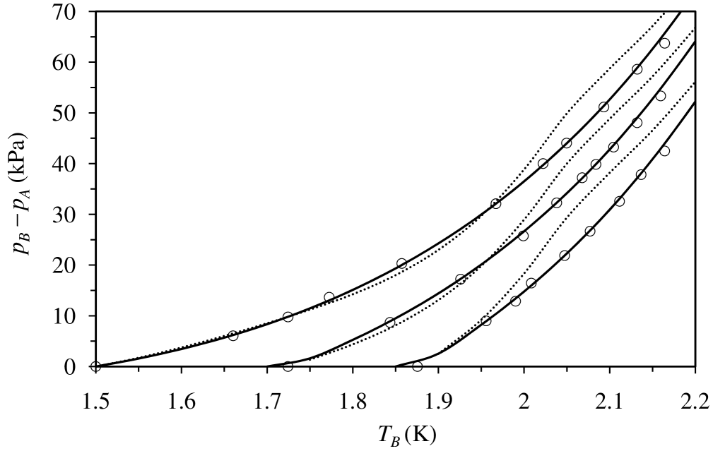
Figure 1: Measured and calculated fountain pressure for $T_{A}=$ 1.502 K (left), 1.724 K (middle), and 1.875 K (right). The symbols are measured data,Hammel61 the full curve is the saturation line integral form of the H. London expression, Eq. (2.15),HLondon39 and the dotted curve is for fixed chemical potential using the incompressible fluid estimate for its departure from the saturation value, Eq. (2.19). The calculated curves use measured saturation data from Ref. Donnelly98, .

Figure 1 tests the various equations for the fountain pressure against the measured values.Hammel61 The calculations use measured data for ⁴He on the saturation curve, including the calorimetrically measured entropy.Donnelly98 The chemical potential for Eq. (2.19) was obtained from the measured enthalpy and entropy.

It can be seen that the H. London expression for the temperature derivative of the fountain pressure, evaluated as an integral along the fountain curve, Eq. (2.15), is practically indistinguishable from the measured values. Adding the correction for the translation from the fountain path to the saturation path, Eq. (II.2), makes a difference of about $-0.5$% at the highest fountain pressure shown, which would be indistinguishable from the uncorrected result, Eq. (2.15), on the scale of the figure.

The equation for the fountain pressure derived directly from the equality of chemical potential, Eq. (2.19), does not perform as well as the integral form of the H. LondonHLondon39 expression, particularly at higher fountain pressures. This is in part due to the fact that a linear expansion has been used to map from the pressure of the second chamber to the saturation pressure. And in part it is due to measurement error, which is always magnified by single point applications and taking the differences between measured quantities. Integral formulations such as Eq. (2.15) tend to smooth out random measurement error. That the overestimate of the predicted pressure for $T_{B}\gtrsim 2$ K is similar in all three cases despite the differences in fountain pressures of about a factor of three tends to suggest that the error is not due to the linearization approximation. Rather it appears that $\mu_{B}^{\mathrm{sat}}$ is systematically too small, which says that either the measured enthalpy is too small, or else the measured entropy is too large in this regime. Despite the limited accuracy of Eq. (2.19), the agreement with the measured data in Fig. 1 is good enough to confirm the thermodynamic analysis that $\mu_{A}=\mu_{B}$ is mathematically equivalent to $\mathrm{d}p_{B}/\mathrm{d}T_{B}=\rho_{B}s_{B}$.

III Osmotic Pressure in an Incompressible Superfluid

In Appendix B the conventional osmotic pressure for a binary solution is obtained using classical ideal solution theory. That result may be compared and contrasted with the present results for a superfluid obtained similarly at the level of an ideal solution.

Consider a system consisting of two chambers at different temperatures below the condensation temperature and containing ⁴He. We give the free energy for a single chamber, and differentiate it to obtain an expression for the chemical potential. This allows us to equate chemical potentials and to obtain the fountain pressure.

The constrained Helmholtz free energy for a single system with $N_{0}$ ground momentum state bosons and $N_{*}$ excited momentum state bosons is given by Attard22a ; Attard21

$$-\beta F(N_{0}|N,V,T)=\ln\frac{\Lambda^{-3N_{*}}Q}{N_{*}!V^{N_{0}}}+\sum_{l=2}^{\infty}\frac{N_{*}^{l}}{N^{l-1}}g^{(l)}.$$ (3.1)

Here $N=N_{0}+N_{*}$, $\beta\equiv 1/k_{\mathrm{B}}T$, and $\Lambda\equiv\sqrt{2\pi\beta\hbar^{2}/m}$ is the thermal wavelength. The series contains the loop grand potentials, which is a quantum effect that arises from the symmetrization of the wave function. The logarithmic term is the classical or monomer term, and it contains the configuration integral for interacting bosons, $Q(N,V,T)$. Compared to classical statistical mechanics of a binary mixture (see Appendix B), for the condensed boson case there is no $N_{0}!$ in the denominator, and instead of $\Lambda^{3N_{0}}$ there appears $V^{N_{0}}$. These differences are a consequence of the non-locality of the permutations of ground momentum state bosons. Attard22a ; Attard21

We make the incompressible liquid approximation, $V=Nv$. The constrained Gibbs free energy, $G=F+pV$, for chamber $A$ is then given by

$$G(N_{0A}|N_{A},p_{A},T_{A})$$

$$= \beta_{A}^{-1}\left[N_{*A}\ln\frac{N_{*A}\Lambda_{A}^{3}}{N_{A}v_{A}}-N_{*A}-\ln\frac{Q_{A}}{V^{N_{A}}}\right]$$

$$\mbox{ }-\sum_{l=2}^{\infty}\frac{\beta_{A}^{-1}N_{*A}^{l}}{N_{A}^{l-1}}g_{A}^{(l)}+p_{A}N_{A}v_{A}.$$

Recall that $N_{A}=N_{*A}+N_{0A}$.

Now for an incompressible fluid, since $\mu^{\mathrm{ex}}=p^{\mathrm{ex}}v$ (see Appendix B), the derivative of the configuration integral term vanishes,

$$\frac{\partial}{\partial N}\ln\frac{Q(N,V,T)}{V^{N}}$$ (3.3)

$$= \frac{\partial(-\beta F^{\mathrm{ex}}(N,V,T))}{\partial N}+v\frac{\partial(-\beta F^{\mathrm{ex}}(N,V,T))}{\partial V}$$

$$= -\beta\mu^{\mathrm{ex}}+\beta p^{\mathrm{ex}}v=0.$$

This result effectively removes the interactions between the helium-4 atoms, and makes the analysis more or less the same as that for an ideal gas, apart from the way in which the fraction of ground and excited momentum state bosons is calculated or measured. Consequently, inserting the incompressible fluid assumption at this stage of the analysis is a rather serious approximation. It would be better to calculate the chemical potential for interacting atoms, which is quite feasible, and this should be explored in the future.

The derivative of the constrained Gibbs free energy gives the chemical potential, which with the vanishing of the derivative of the configurational integral, is

$$\mu_{0A}\equiv\left(\frac{\partial G_{A}}{\partial N_{0A}}\right)_{N_{*A},p_{A},T_{A}}$$ (3.4)

$$= \frac{-\beta_{A}^{-1}N_{A*}v}{V_{A}}+p_{A}v_{A}+\beta_{A}^{-1}\sum_{l=2}^{\infty}(l-1)\frac{N_{*A}^{l}g_{A}^{(l)}}{N_{A}^{l}}$$

$$= \frac{-f_{*A}}{\beta_{A}}+p_{A}\rho_{A}^{-1}+\beta_{A}^{-1}\sum_{l=2}^{\infty}(l-1)(f_{*A})^{l}g_{A}^{(l)}.$$

Here $f_{*A}=N_{*A}/N_{A}$ is the fraction of bosons in excited states in chamber $A$. One can similarly obtain an expression for the excited state chemical potential,

$$\mu_{*A} = \frac{\partial G_{A}}{\partial N_{*A}}$$

$$= \beta_{A}^{-1}\ln\frac{N_{*A}\Lambda_{A}^{3}}{V_{A}}-\beta_{A}^{-1}\frac{N_{*A}v}{V_{A}}+p_{A}v_{A}$$

$$\mbox{ }+\beta_{A}^{-1}\sum_{l=2}^{\infty}g_{A}^{(l)}\left\{(l-1)\frac{N_{*A}^{l}}{N_{A}^{l}}-l\frac{N_{*A}^{l-1}}{N_{A}^{l-1}}\right\}.$$

In the equilibrium state, $\mu_{0A}=\mu_{*A}$, in which case one must have

$$\ln[f_{*A}\rho_{A}\Lambda_{A}^{3}]=\sum_{l=2}^{\infty}lg_{A}^{(l)}f_{*A}^{l-1}.$$ (3.6)

Since the right hand side is a series of positive terms, one must have that $f_{*A}>1/\rho_{A}\Lambda_{A}^{3}$, which places a lower bound on the fraction of excited state bosons (He I) as $T\rightarrow 0$. This result is predicated on the incompressible liquid, ideal solution approximation and also upon the no mixing approximation.

Similar expressions hold for chamber $B$. Hence equating the chemical potential of the two chambers, $\mu_{0A}=\mu_{0B}$, yields the fountain pressure as

$$p_{A}-p_{B}$$

$$= \rho_{A}k_{\mathrm{B}}T_{A}f_{*A}-\rho_{B}k_{\mathrm{B}}T_{B}f_{*B}$$

$$\mbox{ }-k_{\mathrm{B}}\sum_{l=2}^{\infty}(l-1)\Big{\{}\rho_{A}T_{A}g_{A}^{(l)}f_{*A}^{l}-\rho_{B}T_{B}g_{B}^{(l)}f_{*B}^{l}\Big{\}}.$$

Ignoring the loop terms, and taking into account the fact that the excited momentum state fraction increases with increasing temperature, one sees that the higher temperature chamber has the higher pressure. Again neglecting the loop terms, notice the difference between this and the usual osmotic pressure equation (B.4). It is only in the linear regime that they are the same.

The left hand side can be written as a height difference, $[p_{A}-p_{B}]\rho^{-1}\approx mg[h_{A}-h_{B}]$, where $m$ is the molecular mass. (Note that here $g$ is the acceleration due to gravity, not the specific Gibbs free energy, and $h$ is the height, not the specific enthalpy.)

Extensive calculation of the intensive loop Gaussians $g^{(l)}$ up to $l=7$ have been performed for a Lennard-Jones model of ⁴He,Attard21 ; Attard22a and also for ³He.Attard22c The fraction of excited state bosons following condensation has been calculated in the so-called unmixed approximation. Attard22a These have been used in the present expression for the pressure difference. The $\lambda$-transition in Lennard-Jones helium-4 occurs at $T=0.65$. Attard22a

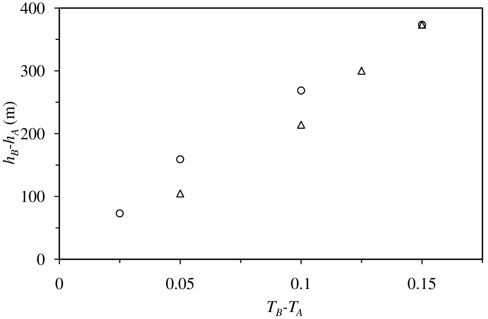
Figure 2: The height difference as a function of the temperature difference for fixed $T_{B}=0.65$ (circles) and for fixed $T_{A}=0.50$ (triangles) for Lennard-Jones ⁴He, for which the temperature in K is $10.22T$.

Figure 2 shows the calculated height difference as a function of the low temperature $T_{A}$ for fixed high temperature $T_{B}=0.65$, which is the $\lambda$- temperature in Lennard-Jones ⁴He. It also shows the height difference for fixed low temperature $T_{A}=0.50$, It can be seen that the height difference increases with increasing temperature difference. The magnitude of the fountain effect is surprisingly large considering that the largest temperature difference shown is about 1.5 K. The loop series contribution to the total height difference is on the order of 1–5%. This means that the major part of the height differences in Fig. 2 come from the first line of the right hand side of Eq. (III), which are essentially ideal solution terms.

It is noticeable in the figure that for the same temperature difference, $T_{B}-T_{A}=0.05$, the higher temperature $T_{B}=0.65$ has a height difference $h_{B}-h_{A}=159.2$ m, which is about 50% larger than that at the lower temperature $T_{A}=0.50$, which has a height difference $h_{B}-h_{A}=104.7$ m. This shows that there is a significant decrease in the ratio of height difference to temperature difference with decreasing temperature. This is because the fraction of excited state bosons decreases with decreasing temperature, and to leading order the height difference is proportional to the difference in the excited fraction.

The experimentally measured value at $T_{A}=1.143$ K is 46.8 m for $T_{B}-T_{A}=0.6$ K.Hammel61 The calculated height difference in Fig. 2 is 104.7 m for $T_{B}-T_{A}=0.05\approx 0.51$ K, which is about a factor of 2 too large. The main reason for the disagreement between the calculated and the measured height difference appears to be the use of the incompressible liquid, ideal solution approximation for the calculations.

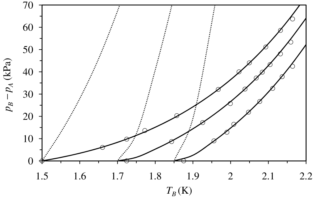
Figure 3: Measured and calculated fountain pressure for $T_{A}=$ 1.502 K (left), 1.724 K (middle), and 1.875 K (right). The symbols are measured data,Hammel61 the full curve is the saturation line integral form of the H. London expression, Eq. (2.15),HLondon39 and the dotted curve uses the incompressible fluid osmotic pressure result, the first line of Eq. (III), using the measured fraction of excited state bosons.Donnelly98 The calculated curves use measured saturation data from Ref. Donnelly98, .

Figure 3 compares the incompressible fluid osmotic pressure result, the first line of Eq. (III), with the measured fountain pressure. This uses the measuredDonnelly98 rather than calculated excited state fraction. It neglects the loop contributions, which as discussed for the previous figure are expected to be small. From the fact that the measured curves are nearly parallel, one can conclude that the fountain pressure is approximately a function of the temperature difference, $T_{B}-T_{A}$, rather than of $T_{B}$ and $T_{A}$ individually. In any case it can be seen that the incompressible, ideal solution result for the osmotic pressure performs quite badly.

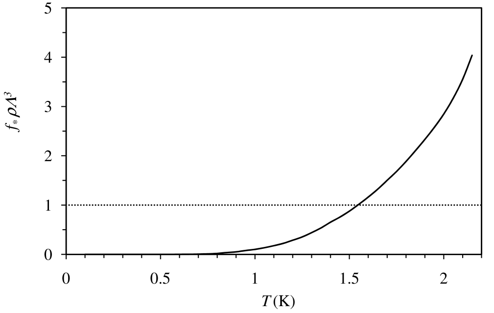
Figure 4: MeasuredDonnelly98 fraction of He I times the measuredDonnelly98 number density and thermal wavelength cubed (solid curve). The dotted line is a guide to the eye.

Figure 4 shows the dimensionless parameter $f_{*}\rho\Lambda^{3}$ using measured data for the fraction of He I. Donnelly98 As discussed following Eq. (3.6), equilibrium between ground and excited state bosons implies that this must be greater than unity, which the figure shows is violated for $T\leq 1.5$ K. The tests of the osmotic pressure prediction for the fountain pressure in Fig. 3 are for $T\geq 1.5$ K. Nevertheless that $f_{*}\rho\Lambda^{3}<1$ for $T\leq 1.5$ K is presumably an indication of the failure of the incompressible liquid, ideal solution, and no mixing approximations in the low temperature regime.

IV Conclusion

The osmotic pressure mechanism offered by TiszaTisza38 as an explanation for the fountain pressure is problematic on physical grounds. In the usual realization of osmotic pressure the solute and the solvent have distinct identities. Hence the only way to equalize the solvent chemical potential is to increase the pressure of the high concentration chamber. In the case of ⁴He, the ground state bosons can become excited state bosons, and vice versa. Hence if the different fractions in each chamber somehow corresponded to a chemical potential difference due to mixing entropy, they could equalize chemical potential simply by changing their state without changing the pressure.

The present calculations show that the osmotic pressure mechanism can be an order of magnitude or more too large for the fountain pressure. Admittedly this is using the incompressible fluid, ideal solution approximation. But since the common understanding of osmotic pressure is that it is due to mixing entropy, and since the latter can be calculated exactly by ideal combinatorics, the failure of the present ideal solution calculations for the fountain pressure argue against osmotic pressure as the physical basis of the fountain effect.

It was found here that H. London’sHLondon39 expression for the temperature derivative of the fountain pressure corresponds to chemical potential equality of the two chambers. This follows from the minimization of energy at constant entropy, which suggests a general principle for superfluid flow and offers an alternative physical explanation for the fountain effect.

Imagine that the high temperature chamber $B$ is initially at saturation. For ⁴He, on the saturation curve the chemical potential from the measuredDonnelly98 enthalpy and entropy decreases with increasing temperature, $\mathrm{d}\mu^{\mathrm{sat}}/\mathrm{d}T<0$. Hence $\mu_{B}^{\mathrm{sat}}<\mu_{A}^{\mathrm{sat}}$. Since $\partial\mu/\partial p=v>0$, the chemical potential of the high temperature chamber can be increased to achieve equality by increasing the pressure beyond its saturation value. This occurs as more bosons arrive in the second chamber because each boson occupies a certain impenetrable volume (i.e. the compressibility is positive). These are the reasons why condensed bosons initially flow down the chemical potential gradient from the low temperature chamber to the high temperature chamber, and why the high temperature chamber subsequently settles at a higher pressure.

One could describe the new principle —that the energy at constant entropy is minimal with respect to particle transfer— as an empirical formula, since the final formula agrees quantitatively with measured results but the axiomatic basis for energy minimization is not well-established. Undoubtedly one could argue that condensed bosons in the superfluid state are in a state of low or zero entropy, and so it would make sense that they respond to mechanical forces rather than to statistical or entropic forces. Also the fact that superfluid flow is flow without viscous dissipation means that the motion of condensed bosons does not produce entropy and so it cannot respond to entropy gradients. And of course condensed bosons in a single quantum state behave as a single particle,Attard21 ; Attard22a which particle responds as a whole to mechanical forces without changing the entropy of the system. Perhaps time and familiarity will raise the status of the present result from empirical to axiomatic.

It is unlikely that the principle of energy minimization at constant entropy is restricted to the fountain effect. Presumably it is a fundamental principle that applies generally for motion without dissipation in Bose-Einstein condensates. As such it provides new insight for the understanding and the analysis of superfluid flow and of superconductor currents.

Appendix A Critique of H. London’s Derivation

As part of the preparation for this paper, a detailed study of H. London’s derivationHLondon39 of his expression was undertaken, and the conclusions are reported here. The criticisms of the derivation are rather serious and suggest a disconnect with the final result. The reader may be sceptical on this point, given the overwhelming experimental evidence for the quantitative accuracy of the H. London expression. And in any case some may wonder whether details of the derivation matter given that the final expression works. But it seems to me that the mathematical derivation does matter because it establishes the status of the final expression: is it a formally exact thermodynamic result, or is it only an accurate approximation? If a theoretical expression is to be used to calibrate instruments, or as a benchmark against which to judge different experimental techniques, then it must be provably exact, not merely an approximation accurate to a limited extent over a limited regime. Establishing the precise status of the H. London expression is particularly important in the case of liquid helium where measured data are reported to four or even more significant figures. Donnelly98

The details of the derivation of H. LondonHLondon39 also matter because they set a precedence for proper thermodynamic manipulation, both in general and in the particular case of superfluid flow. The particular combination of artificial modeling, neglected terms, and implicit assumptions may well give the correct answer on this occasion, but not more generally. Of course since quantitative values of fountain pressure measurements were known to H. London at the time,HLondon39 the fact that his final expression fits the measured data provides little comfort that his derivation of that expression is sound. Presumably to some extent he worked backwards, trying different models and neglecting different terms until he got a result that fitted the known data.

A.1 Artificial Model

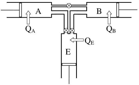
Figure 5: Model system analyzed by H. London.HLondon39

The model used by H. LondonHLondon39 for his derivation of the fountain pressure expression is shown in Fig. 5. In the first half of the cycle, with the valves to the engine closed, the pistons on the chambers are used to transfer $N$ bosons from $A$ to $B$ via the capillary. In the second half of the cycle, sequentially operating the valves and the pistons, the $N$ bosons are transferred back from $B$ to $A$ via the engine following the fountain path $p^{\prime}=p(T^{\prime};p_{A},T_{A})$. Heat flows in to or out of the helium and work is done on or by it at each stage.

The first criticism of H. London’s derivationHLondon39 is the artificiality of this model. What has this got to do with the actual experimental arrangement for measuring the fountain pressure? Are the various heat flows that occur in the artificial engine the same as those that occur in the actual measurement setup? What exactly is superfluid about the model?

My second criticism is that this artificial model seems designed to avoid using an appropriate thermodynamic potential for the system, such as the Helmholtz or Gibbs free energy. These free energies are entirely absent from H. London’s paper.HLondon39 Also absent is the chemical potential, which is the usual thermodynamic variable involved in number exchange.

My third criticism is that the first mention of a specific superfluid property occurs after Eq. (10) of the paper by H. London,HLondon39 which is interpreted to mean that the superfluid has zero entropy. This is after the derivation has been completed; Eq. (11) is the expression for the fountain pressure derivative, the present Eq. (2.1). In neither the model itself or the equations used for the derivation is any restriction or special form due to superfluidity imposed. In other words, the result of the derivation should apply equally to an ordinary fluid. The only way that the correct fountain pressure derivative for a superfluid can emerge from the derivation is by some fortuitous error, or implicit assumption, or neglected contribution.

It is true that early in the derivation H. LondonHLondon39 states that he is treating reversible and irreversible effects as separable and independent, and that he is neglecting the latter. But this is not a property confined to superfluids, since it is a common assumption in irreversible thermodynamics, and it underpins, for example, the formulation of linear hydrodynamics. NETDSM

A.2 Thermodynamic and Mathematical Details

My fourth and final criticism is of the mathematical derivation itself. There are three key equations: the work done by the helium, the change in energy in a cycle, and the change in entropy in a cycle.

H. LondonHLondon39 gives the total work done by the helium in a cycle as his Eq. (1a)

$$W=N\oint_{T_{A}}^{T_{B}}\mathrm{d}T^{\prime}\;v^{\prime}\frac{\mathrm{d}p^{\prime}}{\mathrm{d}T^{\prime}}.$$ (A.1)

The integral is on the fountain path, $p^{\prime}=p(T^{\prime};p_{A},T_{A})$. This equation is correct.

H. LondonHLondon39 defines the heat flow into the helium in chamber $A$ from the reservoir as $Q_{A}$, and similarly for chamber $B$. These neglect any energy change via the capillary.

H. LondonHLondon39 in his Eq. (2) gives the energy conservation equation, otherwise known as the First Law of Thermodynamics, for a full cycle

$$Q_{A}+Q_{B}-N\oint_{T_{A}}^{T_{B}}\mathrm{d}T^{\prime}\;c^{\mathrm{s}}_{p_{A},T_{A}}(T^{\prime})=N\oint_{T_{A}}^{T_{B}}\mathrm{d}T^{\prime}\;v^{\prime}\frac{\mathrm{d}p^{\prime}}{\mathrm{d}T^{\prime}}.$$ (A.2)

Here $c^{\mathrm{s}}_{p_{A},T_{A}}(T^{\prime})=T^{\prime}\mathrm{d}s(T^{\prime};p_{A},T_{A})/\mathrm{d}T^{\prime}$ is the heat capacity per particle along the fountain path (my notation). Here I’ve neglected the thermal conductivity in the capillary, $\mu_{\mathrm{cond}}=0$, as H. London does later in his analysis.HLondon39 The third term on the left hand side is the heat flow into the helium in the engine. Since the energy change in the helium in a full cycle is zero, the heat flow into the helium must equal the work done by the helium. This equation is correct.

In actual fact the integrals can be performed to give

$$Q_{A}+Q_{B}+Nh_{A}-Nh_{B}=0,$$ (A.3)

where $h$ is the enthalpy per particle. It is a little surprising that H. LondonHLondon39 did not avert to this.

H. LondonHLondon39 in his Eq. (3) gives his version of the Second Law of Thermodynamics for the cycle,

$$\frac{Q_{A}}{T_{A}}+\frac{Q_{B}}{T_{B}}-N\oint_{T_{A}}^{T_{B}}\mathrm{d}T^{\prime}\;\frac{c^{\mathrm{s}}_{p_{A},T_{A}}(T^{\prime})}{T^{\prime}}=0.$$ (A.4)

In referring to this equation as the Second Law of Thermodynamics, H. LondonHLondon39 does not appear to be making any statement about entropy maximization. Rather he seems to be making reference to the fact that the heat flow divided by temperature gives a change in entropy.

H. LondonHLondon39 appears to believe that this is an equation for the change in entropy of the subsystems (the chambers) alone, which by definition must be zero for a full cycle. But this equation is not the true equation for the change in entropy of the subsystems as it neglects the work done. Obviously any $pV$-work on a system changes its energy and therefore its entropy; indeed at constant number, $\mathrm{d}S=\mathrm{d}E/T+p\mathrm{d}V/T$. The contribution of the work done by the helium in the chambers in changing their volume is neglected in H. London’sHLondon39 Eq. (3).

Also there is no conservation law for entropy. It is one thing to say that the conserved variables such as energy return to the same state after a full cycle, and that therefore flows in them have to add to zero; it is quite another thing to attempt to analyze flows in non-conserved variables such as entropy. I don’t see the point in attempting to analyze the change in entropy in a cycle unless one intends to maximize it, in which case it should be the total entropy of the chambers and the thermal reservoirs, not just of the chambers.

I also point out the very specific model used by H. LondonHLondon39 for performing work on the helium in the chambers. Such mechanical pistons do not change the entropy of the reservoirs external to the chambers. If one used a more realistic model for the external work, such as the Gibs free energy to represent fluid external to that part of the chamber that is the focus, then one would have to take into account the change in external entropy as work was done on the helium in the chamber. In this case one does not arrive at H. London’sHLondon39 result for the temperature derivative of the fountain pressure.

In summary, whilst I do not doubt the validity of the expression for the temperature derivative of the fountain pressure given by H. London,HLondon39 the present Eq. (2.1), I have grave misgivings about the derivation he offers for it. A theory has to be convincing on its own mathematical and axiomatic merits. A theory cannot be justified by agreement with experiment when the process of developing the end product consists of tinkering with the derivation and model until a fitting result is obtained. Is the successful ‘best fit’ selected for publication any more convincing than those models that didn’t make it?

In the case of H. London’s formula,HLondon39 I find his derivation flawed on several grounds. It appears to me that the combination of the artificial cycle, the unrealistic mechanical external work, the accident that the incorrect expression for the change in entropy of the chambers actually equals the correct expression for the change in the thermal reservoirs, all conspire to give the known experimental result for the fountain pressure even though no superfluid property is actually input into the derivation. Because of these flaws in the derivation, the exact status of the H. LondonHLondon39 formula for the fountain pressure is in my opinion unproven.

Appendix B Incompressible Classical Ideal Gas

Consider two chambers, $A$ and $B$, connected by a semi-permeable membrane transparent to the solvent 1. Assume that the solvent and solute are incompressible, so that the the volume of the first chamber is $V_{A}=N_{A1}v_{1}+N_{A2}v_{2}$, and similarly for the second chamber. The total number is fixed, $N_{n}=N_{An}+N_{Bn}$, $n=1,2$. For the classical ideal gas, the constrained Gibbs free energy is given byTDSM

$$\beta G(N_{A1}|\underline{N},p_{A},p_{B},T)$$

$$= \sum_{n=1}^{2}\Big{\{}N_{An}\ln\frac{N_{An}\Lambda^{3}}{N_{A1}v_{1}+N_{A2}v_{2}}-N_{An}$$

$$\mbox{ }+N_{Bn}\ln\frac{N_{Bn}\Lambda^{3}}{N_{B1}v_{1}+N_{B2}v_{2}}-N_{Bn}\Big{\}}$$

$$\mbox{ }+\beta p_{A}[N_{A1}v_{1}+N_{A2}v_{2}]+\beta p_{B}[N_{B1}v_{1}+N_{B2}v_{2}].$$

Here $\beta=1/k_{\mathrm{B}}T$ is the reciprocal temperature, $\Lambda=\sqrt{2\pi\hbar^{2}\beta/m}$ is the thermal wavelength, $m$ is the mass, and $\mu$ is the chemical potential. Since $G=\mu N$, this shows that for an incompressible fluid, $\mu^{\mathrm{ex}}=p^{\mathrm{ex}}v$. The derivative is

$$\left(\frac{\partial\beta G}{\partial N_{A1}}\right)_{N_{1}} = \ln\frac{N_{A1}\Lambda^{3}}{N_{A1}v_{1}+N_{A2}v_{2}}-\ln\frac{N_{B1}\Lambda^{3}}{N_{B1}v_{1}+N_{B2}v_{2}}$$ (B.2)

$$\mbox{ }-\frac{N_{A1}v_{1}}{N_{A1}v_{1}+N_{A2}v_{2}}+\frac{N_{B1}v_{1}}{N_{B1}v_{1}+N_{B2}v_{2}}$$

$$\mbox{ }-\frac{N_{A2}v_{1}}{N_{A1}v_{1}+N_{A2}v_{2}}+\frac{N_{B2}v_{1}}{N_{B1}v_{1}+N_{B2}v_{2}}$$

$$\mbox{ }+\beta p_{A}v_{1}-p_{B}\beta v_{1}$$

$$= \ln\frac{\rho_{A1}}{\rho_{B1}}-[\rho_{A1}+\rho_{A2}-\rho_{B1}-\rho_{B2}]v_{1}$$

$$\mbox{ }+\beta[p_{A}-p_{B}]v_{1}.$$

Hence at equilibrium

$$\ln\frac{\overline{\rho}_{A1}}{\overline{\rho}_{B1}}-[\overline{\rho}_{A1}+\overline{\rho}_{A2}-\overline{\rho}_{B1}-\overline{\rho}_{B2}]v_{1}v_{1}=-\beta[p_{A}-p_{B}]v_{1}.$$ (B.3)

For simplicity choose $v_{1}=v_{2}=v$, so that $\rho=\rho_{1}+\rho_{2}=v^{-1}$ and $\rho_{A}=\rho_{B}$. In this case the equilibrium condition becomes

$$\ln\frac{\overline{\rho}_{A1}}{\overline{\rho}_{B1}}=\frac{-\beta}{\rho}[p_{A}-p_{B}].$$ (B.4)

Hence $p_{A}\geq p_{B}$ implies that $\overline{\rho}_{A1}\leq\overline{\rho}_{B1}$. The chamber with the greater pressure is the one with the lower solvent fraction (and hence higher solute fraction). This is the classical osmotic pressure.

Appendix C Irreversible Heat Flow

The body of the paper has been concerned with the reversible contributions to the fountain effect, which determine the structure and pressures of the two chambers. It is also of interest to explore at an elementary level of approximation the irreversible contributions, which determine the heat flow in the steady state.

Assuming the enthalpy of the packet is constant, then for $N$ bosons making the passage $A\rightarrow B$ via the capillary the heat flow into the helium is

$$Q_{B}^{\mathrm{irrev}} \approx Nu_{B}-[Nu_{A}-(p_{B}-p_{A})Nv].$$ (C.1)

This assumes that changes in the volume per boson can be neglected. Assuming that the initial energy per particle of the packet is representative of the chamber as a whole, $u_{0A}\approx u_{A}$, allows the irreversible heat flow in the starting chamber to be taken to be zero, $Q_{A}^{\mathrm{irrev}}=0$. Obviously these approximations could be refined.

For the return passage $B\rightarrow A$ via the capillary, the irreversible heat flow is

$$Q_{A}^{\mathrm{irrev}} \approx Nu_{A}-[Nu_{B}+(p_{B}-p_{A})Nv].$$ (C.2)

Again the starting energy is taken to be representative, $u_{0B}\approx u_{B}$, and the irreversible heat flow in the starting chamber is set to zero, $Q_{B}^{\mathrm{irrev}}=0$.

Now the change in entropy of the universe upon cycling a packet of $N$ bosons between the chambers is

$$\frac{\Delta^{\mathrm{irrev}}S_{\mathrm{tot}}}{N} = \frac{-Q_{B}^{\mathrm{irrev}}}{NT_{B}}+\frac{-Q_{A}^{\mathrm{irrev}}}{NT_{A}}$$

$$\approx [u_{B}-u_{A}+(p_{B}-p_{A})v]\frac{T_{B}-T_{A}}{T_{A}T_{B}}.$$

Since both the energy and the pressure increase with temperature, this is positive and quadratic in the temperature difference, as it must be. In the steady state, this drives simultaneous forward and backward superfluid flow in the capillary.

References

- (1) J. F. Allen and H. Jones, “New Phenomena Connected with Heat Flow in Helium II”, Nature 141, 243 (1938).
- (2) S. Balibar “Laszlo Tisza and the Two-Fluid Model of Superfluidity”, C. R. Physique 18, 586 (2017).
- (3) R. J. Donnelly and C. F. Barenghi, “The Observed Properties of Liquid Helium at the Saturated Vapor Pressure”, J. Phys. and Chem. Ref. Data 27, 1217 (1998).
- (4) L. Tisza, “Transport Phenomena in Helium II”, Nature 141, 913 (1938).
- (5) F. London, “The -Phenomenon of Liquid Helium and the Bose-Einstein Degeneracy”, Nature 141, 643 (1938).
- (6) H. London, “Thermodynamics of the Thermomechanical Effect of Liquid He II” Proc. Roy. Soc. A171, 484 (1939).
- (7) E. F. Hammel, Jr. and W. E. Keller, “Fountain Pressure Measurements in Liquid He II”, Phys. Rev. 124, 1641 (1961).
- (8) P. Attard, Quantum Statistical Mechanics in Classical Phase Space (IOP Publishing, Bristol, 2021).
- (9) P. Attard, “Bose-Einstein Condensation, the Lambda Transition, and Superfluidity for Interacting Bosons”, arXiv:2201.07382 (2022).
- (10) P. Attard, “Attraction Between Electron Pairs in High Temperature Superconductors”, arXiv:2203.02598 (2022).
- (11) P. Attard, “New Theory for Cooper Pair Formation and Superconductivity”, arXiv:2203.12103v2 (2022).
- (12) P. Attard, Thermodynamics and Statistical Mechanics: Equilibrium by Entropy Maximisation (Academic Press, London, 2002).
- (13) P. Attard, Non-Equilibrium Thermodynamics and Statistical Mechanics: Foundations and Applications (Oxford University Press, Oxford, 2012).