Parameterized Bipartite Entanglement Measure

Abstract

We propose a novel parameterized entanglement measure $\alpha$-concurrence for bipartite systems. By employing positive partial transposition and realignment criteria, we derive analytical lower bounds for the $\alpha$-concurrence. Moreover, we calculate explicitly the analytic expressions of the $\alpha$-concurrence for isotropic states and Werner states.

I introduction

As a distinguishing feature of quantum mechanics, quantum entanglement is an important resource schrodinger1935gegenwartige ; PhysRev.47.777 ; PhysPhys195 in quantum computation and quantum information processing nielsen2002quantum such as quantum dense coding PhysRevLett.69.2881 , clock synchronization PRL852010 , quantum teleportation PhysRevLett.70.1895 , quantum secret sharing PhysRevA.59.1829 and quantum cryptography PRL67661 . One of the problems in quantum entanglement theory is to quantify the entanglement of a bipartite system. A reasonable entanglement measure $E$ should fulfill PhysRevLett.78.2275 ; PhysRevA.57.1619 ; PhysRevA.56.R3319 ; PhysRevA.59.141 ; PRL842014 : (E1) $E\left(\rho\right)\geqslant 0$, with the equality holding iff $\rho$ is separable; (E2) $E$ is convex, i.e., $E\left(t\rho+\left(1-t\right)\sigma\right)\leqslant tE\left(\rho\right)+\left(1-t\right)E\left(\sigma\right)$ for any states $\rho$ and $\sigma$, where $t\in[0,1]$; (E3) $E$ does not increase under local operation and classical communication (LOCC), i.e., $E\left(\rho\right)\geqslant E\left(\Lambda\left(\rho\right)\right)$ for any completely positive and trace preserving (CPTP) LOCC $\Lambda$; (E4) $E$ does not increase on average under stochastic LOCC, i.e., $E\left(\rho\right)\geqslant\sum_{k}p_{k}E\left(\rho_{k}\right)$, where $p_{k}=\mathrm{Tr}A_{k}\rho A_{k}^{\dagger}$, $\rho_{k}=A_{k}\rho A_{k}^{\dagger}/p_{k}$ and $A_{k}$ are the Kraus operators such that $\sum_{k}A_{k}^{\dagger}A_{k}=I$ with $I$ the identity.

Several reasonable entanglement measures have been presented in the past few years, such as concurrence PhysRevLett.78.5022 ; PhysRevA.64.042315 , entanglement of formation PhysRevA.54.3824 ; PhysRevLett.80.2245 ; horodecki2001entanglement , negativity PhysRevA.65.032314 ; PhysRevLett.95.090503 and Rényi-$\alpha$ entropy of entanglement gour2007dual ; Kim_2010 . Generally it is formidably difficult to calculate analytically the degree of entanglement for arbitrary given states. Analytical results are often available for two-qubit states PhysRevLett.80.2245 or special higher-dimensional mixed states PhysRevLett.85.2625 ; PhysRevA.64.062307 ; PhysRevA.67.012307 for several entanglement measures PhysRevA.68.062304 ; buchholz2016evaluating . Efforts have been also made towards the analytical lower bounds of entanglement measures like the concurrence PhysRevLett.95.210501 ; Li_Guo_2009 . In PhysRevLett.95.040504 analytical lower bound of the concurrence has been derived by employing the positive partial transpose (PPT) and realignment criteria PhysRevLett.77.1413 ; PhysRevA.59.4206 ; rudolph2004computable ; rudolph2005further ; chen2003matrix . In this paper, inspired by Tsallis-$q$ entropy of entanglement raggio1995properties ; PhysRevA.81.062328 and parameterized entanglement monotone $q$-concurrence PhysRevA.103.052423 , we propose a novel parameterized entanglement measure $\alpha$-concurrence for any $0\leqslant\alpha\leqslant 1/2$. Based on PPT and realignment criteria, we also obtain an analytic lower bound of the $\alpha$-concurrence for general bipartite systems. Finally, we calculate the $\alpha$-concurrence of isotropic states and Werner states analytically.

II $\alpha$-concurrence

Let $\mathcal{H}_{A}\otimes\mathcal{H}_{B}$ be an arbitrary $d\times d$ dimensional bipartite Hilbert space associated with subsystems $A$ and $B$. Any pure state on the $\mathcal{H}_{A}\otimes\mathcal{H}_{B}$ can be written as in the Schmidt form,

$$\ket{\psi}=\sum_{i=1}^{r}\sqrt{\lambda_{i}}\ket{a_{i}b_{i}},$$ (1)

where $\sum_{i=1}^{r}\lambda_{i}=1$ with $\lambda_{i}>0$, $r$ is the Schmidt rank, $1\leqslant r\leqslant d$. $\left\{\ket{a_{i}}\right\}$ and $\left\{\ket{b_{i}}\right\}$ are the local bases associated with the subsystems $A$ and $B$, respectively nielsen2002quantum .

$\mathit{Definition}$. For any pure state $\ket{\psi}$ given in (1), the $\alpha$-concurrence is defined by

$$C_{\alpha}\left(\ket{\psi}\right)=\mathrm{Tr}\rho_{A}^{\alpha}-1$$ (2)

for any $0\leqslant\alpha\leqslant 1/2$, where $\rho_{A}=\mathrm{Tr}_{B}|\psi\rangle\langle\psi|$.

From (2), for a pure state $\ket{\psi}$ given by (1) one has

$$C_{\alpha}\left(\ket{\psi}\right)=\sum_{i=1}^{r}\lambda_{i}^{\alpha}-1,$$ (3)

where $C_{\alpha}\left(\ket{\psi}\right)$ satisfies $0\leqslant C_{\alpha}\left(\ket{\psi}\right)\leqslant d^{1-\alpha}-1$. It is obvious that the lower bound is attained if and only if $\ket{\psi}$ is a separable state, that is, $\ket{\psi}=\ket{a_{i}b_{i}}$ for some $\ket{a_{i}}$ and $\ket{b_{i}}$. While the upper bound is achieved for the maximally entangled pure states $\ket{\Psi^{+}}=\frac{1}{\sqrt{d}}\sum_{i=1}^{d}\ket{a_{i}b_{i}}$.

For a general mixed state $\rho$ on the Hilbert space $\mathcal{H}_{A}\otimes\mathcal{H}_{B}$, the $\alpha$-concurrence is given by the convex-roof extension,

$$C_{\alpha}\left(\rho\right)=\min_{\left\{p_{i},\ket{\psi_{i}}\right\}}\sum_{i}p_{i}C_{\alpha}\left(\ket{\psi_{i}}\right),$$ (4)

where the infimum is taken over all possible pure-state decompositions of $\rho=\sum_{i}p_{i}|\psi_{i}\rangle\langle\psi_{i}|$, with $\sum_{i}p_{i}=1$ and $p_{i}>0$. Before showing that $C_{\alpha}\left(\rho\right)$ defined in (4) is indeed a bona fide entanglement measure, we first present the following lemma, see proof in Appendix A.

$\mathit{Lemma\ 1}$. The function $F_{\alpha}\left(\rho\right)=\mathrm{Tr}\rho^{\alpha}-1$ is concave, that is,

$$F_{\alpha}\left(\sum_{i}p_{i}\rho_{i}\right)\geqslant\sum_{i}p_{i}F_{\alpha}\left(\rho_{i}\right)$$ (5)

for any $0\leqslant\alpha\leqslant 1/2$, where $\set{p_{i}}$ is a probability distribution and $\rho_{i}$ are density matrices. The equality holds if and only if all $\rho_{i}$ are the same for all $p_{i}>0$.

By using the above Lemma 1, we have the following theorem.

$\mathit{Theorem\,1}$. The $\alpha$-concurrence $C_{\alpha}\left(\rho\right)$ given in (4) is a well defined parameterized entanglement measure.

$\mathit{Proof}$. We need to verify that $C_{\alpha}\left(\rho\right)$ fulfills the following four requirements.

(E1) If $\rho$ is an entangled state, then there is at least one entangled pure state $\ket{\psi}$ in any pure state decomposition of $\rho$. Thus $C_{\alpha}\left(\rho\right)>0$. Otherwise, $C_{\alpha}\left(\rho\right)=0$ for separable states.

(E2) Consider $\rho=t\rho_{1}+\left(1-t\right)\rho_{2}$. Let $\rho_{1}=\sum_{i}p_{i}|\psi_{i}\rangle\langle\psi_{i}|$ ($\rho_{2}=\sum_{j}q_{j}|\phi_{j}\rangle\langle\phi_{j}|$) be the optimal pure state decomposition of $C_{\alpha}\left(\rho_{1}\right)$ ($C_{\alpha}\left(\rho_{2}\right)$) with $\sum_{i}p_{i}=1$ ($\sum_{j}q_{j}=1$) and $p_{i}>0$ ($q_{j}>0$). We have

$$C_{\alpha}\left(\rho\right) \leqslant\sum_{i=1}^{k}tp_{i}C_{\alpha}\left(\ket{\psi_{i}}\right)+\sum_{j=1}^{l}\left(1-t\right)q_{j}C_{\alpha}\left(\ket{\phi_{j}}\right)$$

$$=tC_{\alpha}\left(\rho_{1}\right)+\left(1-t\right)C_{\alpha}\left(\rho_{2}\right),$$ (6)

where the first inequality is due to that $\sum_{i=1}^{k}tp_{i}|\psi_{i}\rangle\langle\psi_{i}|+\sum_{j=1}^{l}\left(1-t\right)q_{j}|\phi_{j}\rangle\langle\phi_{j}|$ is also a pure state decomposition of $\rho$.

(E3) We adopt the approach given in MINTERT2005207 to show that our entanglement measure does not increase under LOCC. Denote $\vec{\lambda}_{\psi}$ ($\vec{\lambda}_{\phi}$) the Schmidt vector given by the squared Schmidt coefficients of the state $\ket{\psi}$ ($\ket{\phi}$) in the decreasing order. It has been shown that the state $\ket{\phi}$ can be prepared starting from the state $\ket{\psi}$ under LOCC if and only if $\vec{\lambda}_{\psi}$ is majorized by $\vec{\lambda}_{\phi}$ PhysRevLett.83.436 , $\vec{\lambda}_{\psi}\prec\vec{\lambda}_{\phi}$, where the majorization means that the components $\left[\lambda_{\psi}\right]_{i}$ ($\left[\lambda_{\phi}\right]_{i}$) of $\vec{\lambda}_{\psi}$ ($\vec{\lambda}_{\phi}$), listed in nonincreasing order, satisfy $\sum_{i=1}^{j}\left[\lambda_{\psi}\right]_{i}\leqslant\sum_{i=1}^{j}\left[\lambda_{\phi}\right]_{i}$ for $1<j\leqslant d$, with equality for $j=d$.

Since the entanglement cannot increase under LOCC, any entanglement measure $E$ has to satisfy that $E\left(\psi\right)\geqslant E\left(\phi\right)$ whenever $\vec{\lambda}_{\psi}\prec\vec{\lambda}_{\phi}$. This condition, known as the $\mathit{Schur\,concavity}$, is satisfied if and only if $E$, given as a function of the squared Schmidt coefficients $\lambda_{i}$’s ANDO1989163 , is invariant under the permutations of any two arguments and satisfies

$$\left(\lambda_{i}-\lambda_{j}\right)\left(\frac{\partial E}{\partial\lambda_{i}}-\frac{\partial E}{\partial\lambda_{j}}\right)\leqslant 0$$ (7)

for any two components $\lambda_{i}$ and $\lambda_{j}$ of $\vec{\lambda}$.

For any pure state $\ket{\psi}$ given by (1), the $\alpha$-concurrence is obviously invariant under the permutations of the Schmidt coefficients for any $0\leqslant\alpha\leqslant 1/2$. Since

$$\left(\lambda_{i}-\lambda_{j}\right)\left(\frac{\partial C_{\alpha}}{\partial\lambda_{i}}-\frac{\partial C_{\alpha}}{\partial\lambda_{j}}\right)$$

$$=\alpha\left(\lambda_{i}-\lambda_{j}\right)\left(\lambda_{i}^{\alpha-1}-\lambda_{j}^{\alpha-1}\right)\leqslant 0$$

for any two components $\lambda_{i}$ and $\lambda_{j}$ of the squared Schmidt coefficients of $\ket{\psi}$, we have $C_{\alpha}\left(\ket{\psi}\right)\geqslant C_{\alpha}\left(\Lambda\ket{\psi}\right)$ for any LOCC $\Lambda$ and $0\leqslant\alpha\leqslant 1/2$.

Next let $\rho=\sum_{i}p_{i}|\psi_{i}\rangle\langle\psi_{i}|$ be the optimal pure state decomposition of $C_{\alpha}\left(\rho\right)$ with $\sum_{i}p_{i}=1$ and $p_{i}>0$. We obtain

$$C_{\alpha}\left(\rho\right) =\sum_{i}p_{i}C_{\alpha}\left(\ket{\psi_{i}}\right)$$

$$\geqslant\sum_{i}p_{i}C_{\alpha}\left(\Lambda\ket{\psi_{i}}\right)$$

$$\geqslant C_{\alpha}\left(\Lambda\left(\rho\right)\right)$$

for any $0\leqslant\alpha\leqslant 1/2$, where the last inequality is from the definition (4).

(E4) Let $\rho=\sum_{i}p_{i}|\psi_{i}\rangle\langle\psi_{i}|$ be the optimal pure state decomposition of $C_{\alpha}\left(\rho\right)$ with $\sum_{i}p_{i}=1$ and $p_{i}>0$. Consider stochastic LOCC protocol given by Kraus operators $A_{k}$ with $\sum_{k}A_{k}^{\dagger}A_{k}=I$. We have

$$C_{\alpha}\left(\rho\right) =\sum_{i}p_{i}C_{\alpha}\left(\ket{\psi_{i}}\right)$$

$$\geqslant\sum_{i,k}p_{i}p_{k|i}C_{\alpha}\left(\ket{\psi_{i}^{k}}\right)$$

$$=\sum_{i,k}p_{k}p_{i|k}C_{\alpha}\left(\ket{\psi_{i}^{k}}\right)$$

$$=\sum_{k}p_{k}\left(\sum_{i}p_{i|k}C_{\alpha}\left(\ket{\psi_{i}^{k}}\right)\right)$$

$$\geqslant\sum_{k}p_{k}C_{\alpha}\left(\rho^{k}\right),$$ (8)

where $p_{k|i}=\mathrm{Tr}A_{k}|\psi_{i}\rangle\langle\psi_{i}|A_{k}^{\dagger}$ is the probability of obtaining the outcome $k$ with $\ket{\psi_{i}^{k}}=A_{k}\ket{\psi_{i}}/\sqrt{p_{k|i}}$, and $p_{k}=\mathrm{Tr}A_{k}\rho A_{k}^{\dagger}$ is the probability of obtaining the outcome $k$ with $\rho^{k}=A_{k}\rho A_{k}^{\dagger}/p_{k}$. The first inequality is due to the concavity of the Lemma 1, since $\mathrm{Tr}_{B}|\psi_{i}\rangle\langle\psi_{i}|=\sum_{k}p_{k|i}\mathrm{Tr}_{B}|\psi_{i}^{k}\rangle\langle\psi_{i}^{k}|$. The last inequality is from the definition of (4), since $\sum_{i}p_{i|k}|\psi_{i}^{k}\rangle\langle\psi_{i}^{k}|=\rho^{k}$. $\hfill\qed$

In PhysRevA.103.052423 the parameterized entanglement monotone $q$-concurrence $C_{q}\left(\ket{\psi}\right)$ for any pure state $\ket{\psi}$ defined in (1) has been introduced, $C_{q}\left(\ket{\psi}\right)=1-\mathrm{Tr}\rho_{A}^{q}$, where $q\geqslant 2$. It seems that our $\alpha$-concurrence defined by (2), $C_{\alpha}\left(\ket{\psi}\right)=\mathrm{Tr}\rho_{A}^{\alpha}-1$, is in some sense dual to the $q$-concurrence as the parameter $\alpha\in[0,1/2]$, while the parameter $q\geqslant 2$. Nevertheless, these two concurrences characterize the quantum entanglement in different aspects, even though they are both derived from the Tsallis-$q$ of entanglement PhysRevA.81.062328 . For large enough $q$, the $q$-concurrence $C_{q}(\rho)$ converges to the constant $1$ for any entangled state $\rho$, while the $\alpha$-concurrence $C_{\alpha}(\rho)$ not for any $\alpha\in[0,1/2]$. Particularly, for $\alpha=0$, the measure $C_{0}\left(\ket{\psi}\right)=r-1$ for any pure state $\ket{\psi}$ given in (1), where $r$ is the Schmidt rank of the state $\ket{\psi}$, which is solely determined by the Schmidt rank of the bipartite pure state $\ket{\psi}$. Therefore, the $\alpha$-concurrences with different $\alpha$ provide different characterizations of the feature of entanglement.

III bounds on $\alpha$-concurrence

Owing to the optimization in the calculation of the entanglement measures, it is generally difficult to obtain analytical expressions of the entanglement measures for general mixed states. In this section, we derive analytical lower bounds for the $\alpha$-concurrence based on PPT and realignment criteria PhysRevLett.77.1413 ; HORODECKI19961 ; PhysRevA.59.4206 ; rudolph2004computable ; rudolph2005further ; chen2003matrix .

A bipartite state can be written as $\rho=\sum_{ijkl}\rho_{ij,kl}|ij\rangle\langle kl|$, where the subscripts $i$ and $k$ are the row and column indices for the subsystem $A$, respectively, while $j$ and $l$ are such indices for the subsystem $B$. The PPT criterion says that if the state $\rho$ is separable, then the partial transposed matrix $\rho^{\Gamma}=\sum_{ijkl}\rho_{ij,kl}|il\rangle\langle kj|$ with respect to the subsystem $B$ is non-negative, $\rho^{\Gamma}\geqslant 0$. While the realignment criterion says that the realigned matrix of $\rho$, $\mathcal{R}\left(\rho\right)=\sum_{ijkl}\rho_{ij,kl}|ik\rangle\langle jl|$, satisfies that $\|\mathcal{R}\left(\rho\right)\|_{1}\leqslant 1$ if $\rho$ is separable, where $\|X\|_{1}$ denotes the trace norm of matrix $X$, $\|X\|_{1}=\mathrm{Tr}\sqrt{XX^{\dagger}}$.

For a pure state $\ket{\psi}$ given by (1), it is straightforward to obtain that PhysRevLett.95.040504

$$1\leqslant\left\|\rho^{\Gamma}\right\|_{1}=\left\|\mathcal{R}\left(\rho\right)\right\|_{1}=\left(\sum_{i=1}^{r}\sqrt{\lambda_{i}}\right)^{2}\leqslant r,$$ (9)

where $\rho=|\psi\rangle\langle\psi|$. In particular, for $\alpha=1/2$, the $1/2$-concurrence becomes $C_{\frac{1}{2}}\left(\ket{\psi}\right)=\sum_{i=1}^{r}\sqrt{\lambda_{i}}-1$. One has then

$$C_{\frac{1}{2}}\left(\ket{\psi}\right)\geqslant\frac{\left\|\rho^{\Gamma}\right\|_{1}-1}{\sqrt{r}+1}$$ (10)

for any pure state $\ket{\psi}$ on the $\mathcal{H}_{A}\otimes\mathcal{H}_{B}$.

$\mathit{Theorem\ 2}$. For any mixed state $\rho$ on the $\mathcal{H}_{A}\otimes\mathcal{H}_{B}$, the $\alpha$-concurrence $C_{\alpha}\left(\rho\right)$ satisfies

$$C_{\alpha}\left(\rho\right)\geqslant\frac{d^{1-\alpha}-1}{d-1}\left[\max\left(\|\rho^{\Gamma}\|_{1},\|\mathcal{R}\left(\rho\right)\|_{1}\right)-1\right].$$ (11)

$\mathit{Proof}$. For a pure state $\ket{\psi}$ given in (1), let us analyze the monotonicity of the following function,

$$g\left(\alpha\right)=\frac{\sum_{i=1}^{r}\lambda_{i}^{\alpha}-1}{r^{1-\alpha}-1}$$ (12)

for any $0\leqslant\alpha\leqslant 1/2$, where $r>1$. The first derivative of $g\left(\alpha\right)$ with respect to $\alpha$ is given by

$$\frac{\partial g}{\partial\alpha} =\frac{G_{r\alpha}}{\left(r^{1-\alpha}-1\right)^{2}},$$ (13)

where

$$G_{r\alpha}=\sum_{i}\lambda_{i}^{\alpha}\ln\lambda_{i}\left(r^{1-\alpha}-1\right)+\left(\sum_{i}\lambda_{i}^{\alpha}-1\right)r^{1-\alpha}\ln r.$$ (14)

Employing the Lagrange multiplies PhysRevA.67.012307 under constraints $\sum_{i=1}^{r}\lambda_{i}=1$ and $\lambda_{i}>0$, one has that there is only one stable point $\lambda_{i}=1/r$ for every $i=1,\cdots,r$, for which $G_{r\alpha}=0$ for any $0\leqslant\alpha\leqslant 1/2$. Since the second derivative at this point,

$$\frac{\partial^{2}G_{r\alpha}}{\partial\lambda_{i}^{2}}\Big{|}_{\lambda_{i}=\frac{1}{r}}$$

$$=r^{2-\alpha}\left\{\alpha\left(\alpha-1\right)\ln r+\left(2\alpha-1\right)\left(r^{1-\alpha}-1\right)\right\}$$

$$<0$$ (15)

for any $0\leqslant\alpha\leqslant 1/2$, the maximum extreme value point is just the maximum value point. $g\left(\alpha\right)$ is a decreasing function for any $0\leqslant\alpha\leqslant 1/2$, since $\partial g/\partial\alpha\leqslant 0$.

We have

$$C_{\alpha}\left(\ket{\psi}\right) \geqslant\frac{r^{1-\alpha}-1}{\sqrt{r}-1}C_{\frac{1}{2}}\left(\ket{\psi}\right)$$

$$\geqslant\frac{r^{1-\alpha}-1}{r-1}\left(\|\sigma^{\Gamma}\|_{1}-1\right)$$

$$\geqslant\frac{d^{1-\alpha}-1}{d-1}\left(\|\sigma^{\Gamma}\|_{1}-1\right),$$ (16)

where $\sigma=|\psi\rangle\langle\psi|$, the second inequality is due to (10), the last inequality is due to that $\frac{r^{1-\alpha}-1}{r-1}$ is a decreasing function with respect to $r$. Assume $\rho=\sum_{i}p_{i}|\varphi_{i}\rangle\langle\varphi_{i}|$ is the optimal pure state decomposition for $C_{\alpha}\left(\rho\right)$. Then

$$C_{\alpha}\left(\rho\right) =\sum_{i}p_{i}C_{\alpha}\left(\ket{\varphi_{i}}\right)$$

$$\geqslant\frac{d^{1-\alpha}-1}{d-1}\sum_{i}p_{i}\left(\|\sigma_{i}^{\Gamma}\|_{1}-1\right)$$

$$\geqslant\frac{d^{1-\alpha}-1}{d-1}\left(\|\rho^{\Gamma}\|_{1}-1\right),$$ (17)

where $\sigma_{i}=|\varphi_{i}\rangle\langle\varphi_{i}|$, the last inequality is due to the convex property of the trace norm and $\|\rho^{\Gamma}\|\geq 1$ in (9).

Similar to (III) and (III), we obtain from (9) that

$$C_{\alpha}\left(\rho\right)\geqslant\frac{d^{1-\alpha}-1}{d-1}\left(\|\mathcal{R}\left(\rho\right)\|_{1}-1\right)$$ (18)

for any $0\leqslant\alpha\leqslant 1/2$.

Combining (III) and (18), we complete the proof. $\hfill\qed$

IV $\alpha$-concurrence for Isotropic and Werner states

In this section, we compute the $\alpha$-concurrence for isotropic states and Werner states. Let $E$ be a convex-roof extended quantum entanglement measure. Denote $S$ the set of states and $P$ the set all pure states in $S$. Let $G$ be a compact group acting on $S$ by $\left(U,\rho\right)\mapsto U\rho U^{\dagger}$. Assume that the measure $E$ defined on $P$ is invariant under the operations of $G$. One can define the projection $\mathbf{P}$:$S\rightarrow S$ by $\mathbf{P}\rho=\int dUU\rho U^{\dagger}$ with the standard (normalized) Haar measure $dU$ on $G$, and the function $\eta$ on $\mathbf{P}S$ by

$$\eta\left(\rho\right)=\min\left\{E\left(\ket{\Psi}\right):\ket{\psi}\in P,\,\mathbf{P}|\psi\rangle\langle\psi|=\rho\right\}.$$ (19)

Then for $\rho\in\mathbf{P}S$, we have

$$E\left(\rho\right)=co\left(\eta\left(\rho\right)\right),$$ (20)

where $co\left(f\right)$ is the convex-roof extension of a function $f$. In other words, it is the convex hull of $f$.

IV.1 Isotropic states

The isotropic states $\rho_{F}$ are given by PhysRevA.59.4206 ,

$$\rho_{F}=\frac{1-F}{d^{2}-1}\left(I-|\Psi\rangle\langle\Psi|\right)+F|\Psi\rangle\langle\Psi|,$$ (21)

where $\ket{\Psi}=\frac{1}{\sqrt{d}}\sum_{i=1}^{d}\ket{ii}$ and $F=\braket{\Psi}{\rho_{F}}{\Psi}$. $\rho_{F}$ is separable if and only if $0\leqslant F\leqslant 1/d$ PhysRevLett.85.2625 . Inspired by the techniques adopted in PhysRevLett.85.2625 ; PhysRevA.67.012307 ; PhysRevA.64.062307 ; PhysRevA.68.062304 , we have, see Appendix B,

$$\eta_{\alpha}\left(\rho_{F}\right)=\left(Fd\right)^{1-\alpha}-1$$ (22)

for any $0\leqslant\alpha\leqslant 1/2$, where $F>1/d$.

Obviously, the second derivative of (22) with respect to $F$ is non-positive for any $0\leqslant\alpha\leqslant 1/2$. Hence, $\eta_{\alpha}\left(\rho_{F}\right)$ is concave in the whole regime $F\in\left(1/d,1\right]$. The $C_{\alpha}\left(\rho_{F}\right)$ is the largest convex function that is upper bounded by $\eta_{\alpha}\left(\rho_{F}\right)$, which is constructed in the following way. Find the line that passes through the points $\left(F=1/d,\eta_{\alpha}=0\right)$ and $\left(F=1,\eta_{\alpha}=d^{1-\alpha}-1\right)$ of $\eta_{\alpha}\left(\rho_{F}\right)$ for any $0\leqslant\alpha\leqslant 1/2$. Thus, we have the following analytical formula of the $\alpha$-concurrence for isotropic states.

$\mathit{Lemma\ 2}$. The $\alpha$-concurrence for isotropic states $\rho_{F}\in\mathbb{C}^{d}\otimes\mathbb{C}^{d}\ \left(d\geqslant 2\right)$ is given by

$$C_{\alpha}\left(\rho_{F}\right)=\begin{cases}0,&F\leqslant 1/d,\\[5.69054pt] \displaystyle\frac{d^{1-\alpha}-1}{d-1}\left(dF-1\right),&F>1/d,\end{cases}$$ (23)

where $0\leqslant\alpha\leqslant 1/2$ and $d\geqslant 2$.

Since $\|\rho_{F}^{\Gamma}\|_{1}=\|\mathcal{R}\left(\rho_{F}\right)\|_{1}=Fd$ for $F>1/d$ rudolph2005further ; PhysRevA.65.032314 , surprisingly the lower bound of (11) is just exactly the (23) for every $0\leqslant\alpha\leqslant 1/2$ with $d\geqslant 2$.

The concurrence $C\left(\rho_{F}\right)$ of isotropic states has been derived in PhysRevA.67.012307 , $C\left(\rho_{F}\right)=\sqrt{\frac{2}{d\left(d-1\right)}}\left(dF-1\right)$ for any $F>1/d$. Fig. 1 exhibits the relations between the concurrence and the $\alpha$-concurrence of isotropic states for $\alpha=0$ and $1/2$.

Figure 1: Entanglement of isotropic states. The green (blue) surface stands for $C_{0}\left(\rho_{F}\right)$ ($C_{1/2}\left(\rho_{F}\right)$), the red surface is for the concurrence $C\left(\rho_{F}\right)$.

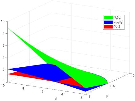
Especially, it shows that the $C_{0}\left(\rho_{F}\right)=C\left(\rho_{F}\right)$ with $d=2$, and the concurrence of isotropic states is less than the $0$-concurrence with $d>2$. Moreover, we notice that the $1/2$-concurrence is bigger than the concurrence with $d\geq 5.1508$.

IV.2 Werner states

The Werner states are of the form,

$$\rho_{W}= \frac{2\left(1-W\right)}{d\left(d+1\right)}\left(\sum_{k=1}^{d}|kk\rangle\langle kk|+\sum_{i<j}|\Psi_{ij}^{+}\rangle\langle\Psi_{ij}^{+}|\right)$$

$$+\frac{2W}{d\left(d-1\right)}\sum_{i<j}|\Psi_{ij}^{-}\rangle\langle\Psi_{ij}^{-}|,$$ (24)

where $\ket{\Psi_{ij}^{\pm}}=(\ket{ij}\pm\ket{ji})/\sqrt{2}$ and $W=\mathrm{Tr}(\rho_{W}\sum_{i<j}|\Psi_{ij}^{-}\rangle\langle\Psi_{ij}^{-}|)$ PhysRevA.68.062304 . $\rho_{W}$ is separable if and only if $0\leqslant W\leqslant 1/2$ PhysRevA.64.062307 ; PhysRevA.40.4277 . For $W>1/2$, we have, see Appendix C,

$$\eta_{\alpha}\left(\rho_{W}\right)=\left(2W\right)^{1-\alpha}-1$$ (25)

for any $0\leqslant\alpha\leqslant 1/2$.

It is direct to verify that the second derivative of (25) with respect to $W$ is non-positive, namely, $\eta_{\alpha}\left(\rho_{W}\right)$ is concave. Similar to (23), we have

$\mathit{Lemma\ 3}$. The $\alpha$-concurrence for Werner states $\rho_{W}\in\mathbb{C}^{d}\otimes\mathbb{C}^{d}\ \left(d\geqslant 2\right)$ is given by

$$C_{\alpha}\left(\rho_{W}\right)=\begin{cases}0,&W\leqslant 1/2,\\[2.84526pt] \left(2^{1-\alpha}-1\right)\left(2W-1\right),&W>1/2,\end{cases}$$ (26)

where $0\leqslant\alpha\leqslant 1/2$.

We remark that for $W>1/2$, the lower bound of (11) for Werner states is given by

$$C_{\alpha}\left(\rho_{W}\right)\geqslant\frac{2\left(d^{1-\alpha}-1\right)}{d\left(d-1\right)}\left(2W-1\right).$$ (27)

Accounting to (26), we obtain

$$\left(2^{1-\alpha}-1\right)\left(2W-1\right)\geqslant\frac{2\left(d^{1-\alpha}-1\right)}{d\left(d-1\right)}\left(2W-1\right),$$ (28)

where equality holds if $d=2$, and the inequality holds strictly for higher dimensional quantum systems.

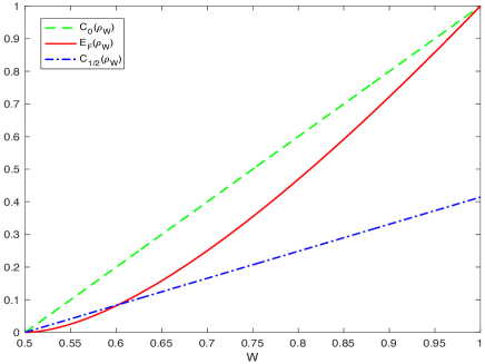
The concurrence of Werner states has been obtained in PhysRevA62044302 , $C\left(\rho_{W}\right)=2W-1$ for $W>1/2$. It is direct to find that $C_{\alpha}\left(\rho_{W}\right)=\left(2^{1-\alpha}-1\right)C\left(\rho_{W}\right)$ for any $0\leq\alpha\leq 1/2$. Moreover, the entanglement of formation for Werner states is given by PhysRevA.64.062307 , $E_{F}\left(\rho_{W}\right)=H_{2}[\frac{1}{2}(1-2\sqrt{W\left(1-W\right)})]$. In Fig. 2 we illustrate the relations among the concurrence, entanglement of formation and $\alpha$-concurrence of Werner states for $\alpha=0$ and $1/2$. The entanglement of formation for Werner states $E_{F}\left(\rho_{W}\right)$ is always upper bounded by the $C_{0}\left(\rho_{W}\right)=C\left(\rho_{W}\right)$, and larger than the $1/2$-concurrence $C_{1/2}\left(\rho_{W}\right)$ for $W\geq 0.6$.

Figure 2: Entanglement for Werner states. The dashed (green) line stands for $C_{0}\left(\rho_{W}\right)=C\left(\rho_{W}\right)$. The solid (red) line is for the entanglement of formation $E_{F}\left(\rho_{W}\right)$, the dot dashed (blue) line is for the $1/2$-concurrence $C_{1/2}\left(\rho_{W}\right)$.

V summary

We have introduced the concept of $\alpha$-concurrence and shown that the $\alpha$-concurrence is a well defined entanglement measure. Analytical lower bounds of the $\alpha$-concurrence for general mixed states have been derived based on PPT and realignment criterion. Specifically, we have derived explicit formulae for the $\alpha$-concurrence of isotropic states and Werner states. Interestingly our lower bounds are exact for isotropic states and Werner states with $d=2$. Our parameterized entanglement measure $\alpha$-concurrence gives a family of entanglement measures and enriches the theory of quantum entanglement, which may highlight further researches on the study of quantifying quantum entanglement and the related investigations like monogamy and polygamy relations in entanglement distribution, as well as the physical understanding of quantum correlations.

Appendix A Proof of Lemma 1

We only need to prove that $F_{\alpha}\left(t\rho+\left(1-t\right)\sigma\right)\geqslant tF_{\alpha}\left(\rho\right)+\left(1-t\right)F_{\alpha}\left(\sigma\right)$ for any $t\in\left[0,1\right]$. Since for any concave function $f$, the $\mathrm{Tr}\left[f\left(\rho\right)\right]$ is also concave RevModPhys.50.221 , $f\left(x\right)=x^{\alpha}$ with $x\in\left[0,1\right]$ is concave for any $0\leqslant\alpha\leqslant 1/2$. Let ${\rho}^{\prime}=t\rho+\left(1-t\right)\sigma=\sum_{j}q_{j}|\phi_{j}\rangle\langle\phi_{j}|$, $\rho=\sum_{i}p_{i}|\psi_{i}\rangle\langle\psi_{i}|$ and $\sigma=\sum_{k}r_{k}|\xi_{k}\rangle\langle\xi_{k}|$ be corresponding eigendecompositions. We have

$$F_{\alpha}\left({\rho}^{\prime}\right) =\sum_{j}\left[t\braket{\phi_{j}}{\rho}{\phi_{j}}+\left(1-t\right)\braket{\phi_{j}}{\sigma}{\phi_{j}}\right]^{\alpha}-1$$

$$\geqslant\sum_{j}\left\{t\braket{\phi_{j}}{\rho}{\phi_{j}}^{\alpha}+\left(1-t\right)\braket{\phi_{j}}{\sigma}{\phi_{j}}^{\alpha}\right\}-1$$

$$=t\sum_{j}\left(\sum_{i}p_{i}|\braket{\phi_{j}}{\psi_{i}}|^{2}\right)^{\alpha}$$

$$\ \ \ +\left(1-t\right)\sum_{j}\left(\sum_{k}r_{k}|\braket{\phi_{j}}{\xi_{k}}|^{2}\right)^{\alpha}-1$$

$$\geqslant t\sum_{i,j}|\braket{\phi_{j}}{\psi_{i}}|^{2}p_{i}^{\alpha}+\left(1-t\right)\sum_{j,k}|\braket{\phi_{j}}{\xi_{k}}|^{2}r_{k}^{\alpha}-1$$

$$=t\sum_{i}p_{i}^{\alpha}+\left(1-t\right)\sum_{k}r_{k}^{\alpha}-1$$

$$=tF_{\alpha}\left(\rho\right)+\left(1-t\right)F_{\alpha}\left(\sigma\right),$$ (29)

where the two inequalities follow from the concavity of $f$. The equality holds if $\rho$ and $\sigma$ are identical. $\hfill\qed$

Appendix B $\eta_{\alpha}$ for Isotropic states

Let $\mathcal{T}_{iso}$ be the $\left(U\otimes U^{*}\right)$-twirling operator defined by $\mathcal{T}_{iso}\left(\rho\right)=\int dU\left(U\otimes U^{\ast}\right)\rho\left(U\otimes U^{\ast}\right)^{\dagger}$, where $dU$ denotes the standard Haar measure on the group of all $d\times d$ unitary operations. Then the operator satisfies that $\mathcal{T}_{iso}\left(\rho\right)=\rho_{F\left(\rho\right)}$ with $F\left(\rho\right)=\braket{\Psi}{\rho}{\Psi}$. One has $\mathcal{T}_{iso}\left(\rho_{F}\right)=\rho_{F}$ PhysRevA.64.062307 ; PhysRevA.59.4206 ; PhysRevA.68.062304 . Applying $\mathcal{T}_{iso}$ to the pure state $\ket{\psi}$ given in (1), $\ket{\psi}=\sum_{i=1}^{r}\sqrt{\lambda_{i}}U_{A}\otimes U_{B}\ket{ii}$ with $\ket{a_{i}}=U_{A}\ket{i}$ and $\ket{b_{i}}=U_{B}\ket{i}$, we have

$$\mathcal{T}_{iso}\left(|\psi\rangle\langle\psi|\right)=\rho_{F\left(|\psi\rangle\langle\psi|\right)}=\rho_{F\left(\vec{\lambda},V\right)},$$ (30)

where $V=U_{A}^{T}U_{B}$ and

$$F\left(\vec{\lambda},V\right)=|\braket{\Psi}{\psi}|^{2}=\frac{1}{d}\Big{|}\sum_{i=1}^{r}\sqrt{\lambda_{i}}V_{ii}\Big{|}^{2}$$ (31)

with $V_{ij}=\braket{i}{V}{j}$, and $\vec{\lambda}$ is the Schmidt vector of (1). Then the function $\eta$ defined in (19) becomes

$$\eta_{\alpha}\left(\rho_{F}\right)=\min_{\set{\vec{\lambda},V}}\left\{C_{\alpha}\left(\vec{\lambda}\right):\frac{1}{d}\Big{|}\sum_{i=1}^{r}\sqrt{\lambda_{i}}V_{ii}\Big{|}^{2}=F\right\}.$$ (32)

It has been proved that the minimum above is attained for $V=I$ PhysRevA.68.062304 . Therefore, we have

$$\eta_{\alpha}\left(\rho_{F}\right)=\min_{\vec{\lambda}}\left\{C_{\alpha}\left(\vec{\lambda}\right):\frac{1}{d}\Big{|}\sum_{i=1}^{r}\sqrt{\lambda_{i}}\Big{|}^{2}=F\right\}.$$ (33)

For $F\in(0,\frac{1}{d}]$, one can always chose suitable $U_{A}$ and $U_{B}$ such that $\lambda_{1}=1$, and hence $\eta_{\alpha}\left(\rho_{F}\right)=0$. For $F\in(\frac{1}{d},1]$, similar to PhysRevA.103.052423 ; PhysRevLett.85.2625 , by using the Lagrange multipliers PhysRevA.67.012307 one can minimize (33) subject to the constraints

$$\sum_{i=1}^{r}\lambda_{i}=1,~{}~{}~{}\sum_{i=1}^{r}\sqrt{\lambda_{i}}=\sqrt{Fd}$$ (34)

with $Fd\geqslant 1$. An extremum is attained when

$$\left(\sqrt{\lambda_{i}}\right)^{2\alpha-1}+\Lambda_{1}\sqrt{\lambda_{i}}+\Lambda_{2}=0,$$ (35)

where $\Lambda_{1}$ and $\Lambda_{2}$ denote the Lagrange multipliers.

It is evident that $f\left(\sqrt{\lambda_{i}}\right)=\left(\sqrt{\lambda_{i}}\right)^{2\alpha-1}$ is a convex function of $\sqrt{\lambda_{i}}$ for any $0\leqslant\alpha\leqslant 1/2$. Since a convex function and a linear function cross at most two points, equation (35) has at most two possible nonzero solutions for $\sqrt{\lambda_{i}}$. Let $\gamma$ and $\delta$ be these two positive solutions with $\gamma>\delta$. The Schmidt vector $\vec{\lambda}=\left\{\lambda_{1},\lambda_{2},\dots,\lambda_{r},0,\cdots,0\right\}$ has the form,

$$\lambda_{j}=\begin{cases}\gamma^{2},&j=1,2,...,n,\\ \delta^{2},&j=n+1,...,n+m,\\ 0,&j=n+m+1,...,d,\end{cases}$$ (36)

where $r=n+m\leqslant d$ and $n\geqslant 1$. The minimization problem of (33) has been reduced to the following minimum problem,

$$\eta_{\alpha}\left(\rho_{F}\right)=\min_{n,m}C_{\alpha}^{nm}\left(F\right)$$ (37)

with

$$C_{\alpha}^{nm}\left(F\right)=n\gamma^{2\alpha}+m\delta^{2\alpha}-1,$$ (38)

subject to the constraints

$$n\gamma^{2}+m\delta^{2}=1,~{}~{}~{}n\gamma+m\delta=\sqrt{Fd}.$$ (39)

By solving Eq. (39), we obtain

$$\gamma_{nm}^{\pm}\left(F\right)=\frac{n\sqrt{Fd}\pm\sqrt{nm\left(n+m-Fd\right)}}{n\left(n+m\right)},$$ (40)

$$\delta_{nm}^{\pm}\left(F\right)=\frac{m\sqrt{Fd}\mp\sqrt{nm\left(n+m-Fd\right)}}{m\left(n+m\right)}.$$ (41)

The relation $\gamma_{nm}^{\pm}\left(F\right)=\delta_{mn}^{\mp}\left(F\right)$ suggests that we only need to consider the cases $\gamma_{nm}:=\gamma_{nm}^{+}\left(F\right)$ and $\delta_{nm}=\delta_{nm}^{+}\left(F\right)$, which are real for $Fd\leqslant n+m$. On the other hand, since $\delta_{nm}$ should be non-negative, we must have $Fd\geqslant n$. Therefore, we see that $\delta_{nm}\leqslant\sqrt{Fd}/\left(n+m\right)\leqslant\gamma_{nm}$, in consistent with the assumption $\gamma>\delta$. Here, $n\geqslant 1$ as $n=0$ is ill defined.

We seek is the minimum of $C_{\alpha}^{nm}\left(F\right)$ over all possible $n$ and $m$, by minimizing $C_{\alpha}^{nm}$ on the parallelogram defined by $1\leqslant n\leqslant Fd$ and $Fd\leqslant n+m\leqslant d$. Note that the parallelogram collapses to a line when $Fd=1$, i.e., the separable boundary. We have $\gamma_{nm}\geqslant\delta_{nm}\geqslant 0$ in the parallelogram. Moreover, $\gamma_{nm}=\delta_{nm}$ if and only if $n+m=Fd$; while $\delta_{nm}=0$ if and only if $n=Fd$.

When $\alpha=1/2$, we see from Eqs. (38) and (39) that Eq. (22) holds without any optimization. When $\alpha=0$, $C_{0}^{nm}\left(F\right)=n+m-1$ and Eq. (22) satisfied with the constraint conditions. From Eq.(39) the derivatives of $\gamma_{nm}$ and $\delta_{nm}$ with respect to $n$ and $m$ are given by,

$$\frac{\partial\gamma}{\partial n} =\frac{1}{2n}\frac{2\gamma\delta-\gamma^{2}}{\gamma-\delta},$$

$$\frac{\partial\delta}{\partial n} =-\frac{1}{2m}\frac{\gamma^{2}}{\gamma-\delta},$$

$$\frac{\partial\delta}{\partial m} =-\frac{1}{2m}\frac{2\gamma\delta-\delta^{2}}{\gamma-\delta},$$

$$\frac{\partial\gamma}{\partial m} =\frac{1}{2n}\frac{\delta^{2}}{\gamma-\delta}.$$ (42)

Hence, using Eq. (38) we have the partial derivatives of $C_{\alpha}^{nm}\left(F\right)$ with respect to $n$ and $m$,

$$\frac{\partial C_{\alpha}^{nm}}{\partial n}=\left(1-\alpha\right)\gamma^{2\alpha}+\alpha\gamma^{2}\delta\frac{\gamma^{2\alpha-2}-\delta^{2\alpha-2}}{\gamma-\delta},$$ (43)

$$\frac{\partial C_{\alpha}^{nm}}{\partial m}=\left(1-\alpha\right)\delta^{2\alpha}+\alpha\delta^{2}\gamma\frac{\gamma^{2\alpha-2}-\delta^{2\alpha-2}}{\gamma-\delta}.$$ (44)

By lengthy calculations, we have

$$\frac{\partial C_{\alpha}^{nm}}{\partial m}=\frac{\delta^{2\alpha+1}}{\gamma-\delta}\left\{\left(1-\alpha\right)\left(\frac{\gamma}{\delta}-1\right)+\alpha\left(\frac{\gamma}{\delta}\right)^{2\alpha-1}-\alpha\frac{\gamma}{\delta}\right\}.$$ (45)

Denote $t=\frac{\gamma}{\delta}$. One has $t\geqslant 1$. Let

$$g\left(t\right)=\left(1-\alpha\right)\left(t-1\right)+\alpha t^{2\alpha-1}-\alpha t.$$ (46)

We have $g\left(1\right)=0$ and

$$\frac{\partial g}{\partial t}=\left(1-2\alpha\right)\left(1-\alpha t^{2\alpha-2}\right).$$ (47)

Set $h\left(t\right)=1-\alpha t^{2\alpha-2}$ with $h\left(1\right)=1-\alpha>0$. We obtain

$$\frac{\partial h}{\partial t}=-\alpha\left(2\alpha-2\right)t^{2\alpha-3}\geqslant 0.$$ (48)

From Eqs. (48) and (47), combining with Eq.(46) we have

$$\frac{\partial C_{\alpha}^{nm}}{\partial m}\geqslant 0.$$ (49)

Now corresponding to moving perpendicularly to and parallel to the $n+m=$constant boundaries of the parallelogram, we make a parameter transformation, $u=n-m$ and $v=n+m$. The derivative of $C_{\alpha}^{nm}$ with respect to $u$ is given by

$$\frac{\partial C_{\alpha}^{nm}}{\partial u}=\frac{1}{2}\left(\frac{\partial C_{\alpha}}{\partial n}-\frac{\partial C_{\alpha}}{\partial m}\right)$$

$$=\frac{1}{2}\left\{\gamma^{2\alpha-1}\left[\left(1-\alpha\right)\gamma+\alpha\delta\right]-\delta^{2\alpha-1}\left[\left(1-\alpha\right)\delta+\alpha\gamma\right]\right\}$$

$$=\frac{\gamma^{2\alpha}}{2}\left\{1-\alpha+\alpha\frac{\delta}{\gamma}-\left(\frac{\delta}{\gamma}\right)^{2\alpha}\left(1-\alpha+\alpha\frac{\gamma}{\delta}\right)\right\}.$$

Set $x=\frac{\delta}{\gamma}$ with $0\leqslant x\leqslant 1$. Let

$$f\left(x\right)=1-\alpha+\alpha x-x^{2\alpha}\left(1-\alpha+\alpha x^{-1}\right)$$ (50)

with $f\left(1\right)=0$. We have the derivative of $f\left(x\right)$ respect to $x$,

$$\frac{\partial f}{\partial x}=\alpha\left\{1-\left[2x^{2\alpha-1}\left(1-\alpha+\alpha x^{-1}\right)-x^{2\alpha-2}\right]\right\}.$$ (51)

Again let

$$k\left(x\right)=2x^{2\alpha-1}\left(1-\alpha+\alpha x^{-1}\right)-x^{2\alpha-2}$$ (52)

with $k\left(1\right)=1$. Then

$$\frac{\partial k}{\partial x}=x^{2\alpha-3}l\left(x\right),$$ (53)

where

$$l\left(x\right)=2\left(2\alpha-1\right)\left(x-\alpha x\right)-\left(1-\alpha\right)\left(4\alpha-2\right).$$ (54)

We have $l\left(1\right)=0$ and

$$\frac{\partial l}{\partial x}=2\left(2\alpha-1\right)\left(1-\alpha\right)\leqslant 0.$$ (55)

From Eqs. (55) and (53), combining Eq. (51) we obtain $\partial f/\partial x\geqslant 0$. Then for any $x\in[0,1]$ we have $f\left(x\right)\leqslant f\left(1\right)=0$. Therefore,

$$\frac{\partial C_{\alpha}^{nm}}{\partial u}\leqslant 0.$$ (56)

From Eqs. (49) and (56), the minimum of $C_{\alpha}^{nm}\left(F\right)$ is obtained when $m$ is the minimum and $u$ is the maximum. These results imply that the minimum of $C_{\alpha}^{nm}\left(F\right)$ occurs at the vertex of $n=Fd$ and $m=0$. Specifically, since $\gamma_{nm}=\delta_{nm}$ on the boundary $n+m=Fd$ where Eqs. (49) and (56) are both hold, we have ${n}^{\prime}=n+m=Fd$ and ${m}^{\prime}=0$. In this way, we derive an analytical expression of the function $\eta_{\alpha}\left(\rho_{F}\right)$ as follows,

$$\eta_{\alpha}\left(\rho_{F}\right)=\left(Fd\right)^{1-\alpha}-1.$$ (57)

Appendix C $\eta_{\alpha}$ for Werner states

Let $\mathcal{T}_{wer}\left(\rho\right)=\int dU\left(U\otimes U\right)\rho\left(U^{\dagger}\otimes U^{\dagger}\right)$ be the $\left(U\otimes U\right)$-twirling transformations PhysRevA.64.062307 . Then the Werner states defined in (IV.2) satisfy that, in analogous to the isotropic states, $\mathcal{T}_{wer}\left(\rho\right)=\rho_{W\left(\rho\right)}$, where $W\left(\rho\right)=\mathrm{Tr}\left(\rho\sum_{i<j}|\Psi_{ij}^{-}\rangle\langle\Psi_{ij}^{-}|\right)$ and $\mathcal{T}_{wer}\left(\rho_{W}\right)=\rho_{W}$ PhysRevA.59.4206 ; PhysRevA.68.062304 . Applying $\mathcal{T}_{wer}$ to the pure state $\ket{\psi}$ defined in (1), $\ket{\psi}=\sum_{i=1}^{r}\sqrt{\lambda_{i}}U_{A}\otimes U_{B}\ket{ii}$, we have

$$\mathcal{T}_{wer}\left(|\psi\rangle\langle\psi|\right)=\rho_{W\left(|\psi\rangle\langle\psi|\right)}=\rho_{W\left(\vec{\lambda},\Lambda\right)},$$ (58)

where $\Lambda=U_{A}^{\dagger}U_{B}$ and

$$W\left(\vec{\lambda},\Lambda\right) =\sum_{i<j}|\braket{\Psi_{ij}^{-}}{\psi}|^{2}$$

$$=\frac{1}{2}\sum_{i<j}|\sqrt{\lambda_{i}}\Lambda_{ji}-\sqrt{\lambda_{j}}\Lambda_{ij}|^{2}$$ (59)

with $\Lambda_{ij}=\braket{i}{\Lambda}{j}$. Then the function $\eta$ defined in (19) becomes

$$\eta_{\alpha}\left(\rho_{W}\right)=\min_{\set{\vec{\lambda},\Lambda}}\left\{C_{\alpha}\left(\vec{\lambda}\right):W\left(\vec{\lambda},\Lambda\right)=W\right\}.$$ (60)

By $W\left(\vec{\lambda},\Lambda\right)=W$ we have

$$2W =1-\sum_{i=1}^{r}\lambda_{i}|\Lambda_{ii}|^{2}-2\sum_{i<j}\sqrt{\lambda_{i}\lambda_{j}}\mathrm{Re}\left(\Lambda_{ij}\Lambda_{ji}^{\ast}\right)$$

$$\leqslant 1+2\sum_{i<j}\sqrt{\lambda_{i}\lambda_{j}}|\mathrm{Re}\left(\Lambda_{ij}\Lambda_{ji}^{\ast}\right)|$$

$$\leqslant 1+2\sum_{i<j}\sqrt{\lambda_{i}\lambda_{j}}$$

$$=|\sum_{i=1}^{r}\sqrt{\lambda_{i}}|^{2},$$ (61)

where $\mathrm{Re}\left(z\right)$ is the real part of $z$.

Note that the equalities in (C) hold if only the two nozero components $\Lambda_{01}=1$ and $\Lambda_{10}=-1$, and $\vec{\lambda}=\left(\lambda_{1},\lambda_{2},0,\cdots,0\right)$, which give rise to the optimal minimum of (60) PhysRevA.64.062307 . Therefore, (60) becomes

$$\eta_{\alpha}\left(\rho_{W}\right)=\min_{\vec{\lambda}}\left\{C_{\alpha}\left(\vec{\lambda}\right):|\sum_{i=1}^{2}\sqrt{\lambda_{i}}|^{2}=2W\right\}.$$ (62)

For $W\in(0,\frac{1}{2}]$, we can always chose suitable $U_{A}$ and $U_{B}$ to have that $\lambda_{1}=1$, which results in $\eta_{\alpha}\left(\rho_{W}\right)=0$. For $W>1/2$, one minimizes (62) subject to the constraints

$$\sum_{i=1}^{2}\lambda_{i}=1,~{}~{}~{}\sum_{i=1}^{2}\sqrt{\lambda_{i}}=\sqrt{2W}$$ (63)

with $W>1/2$. The rest of the calculation is the similar to the one in Appendix B. We only need to set $d=2$ and $F=W$. In this way, we can obtain

$$\eta_{\alpha}\left(\rho_{W}\right)=\left(2W\right)^{1-\alpha}-1.$$ (64)

References

- (1) Schrödinger E 1935 Naturwissenschaften 23 807
- (2) Einstein A, Podolsky B and Rosen N 1935 Phys. Rev. 47 777
- (3) Bell J S 1964 Phys. Phys. Fiz. 1 195
- (4) Nielsen M A and Chuang I L 2010 Quantum Computation and Quantum Information 10th edn (Cambridge: Cambridge University Press)
- (5) Bennett C H and Wiesner S J 1992 Phys. Rev. Lett. 69 2881
- (6) Jozsa R, Abrams D S, Dowling J P and Williams C P 2000 Phys. Rev. Lett. 85 2010
- (7) Bennett C H, Brassard G, Crépeau C, Jozsa R, Peres A and Wootters W K 1993 Phys. Rev. Lett. 70 1895
- (8) Hillery M, Bužek V and Berthiaume A 1999 Phys. Rev. A 59 1829
- (9) Ekert A K 1991 Phys. Rev. Lett. 67 661
- (10) Vedral V, Plenio M B, Rippin M A and Knight P L 1997 Phys. Rev. Lett. 78 2275
- (11) Vedral V and Plenio M B 1998 Phys. Rev. A 57 1619
- (12) Popescu S and Rohrlich D 1997 Phys. Rev. A 56 R3319
- (13) Vidal G and Tarrach R 1999 Phys. Rev. A 59 141
- (14) Horodecki M, Horodecki P and Horodecki R 2000 Phys. Rev. Lett. 84 2014
- (15) Hill S and Wootters W K 1997 Phys. Rev. Lett. 78 5022
- (16) Rungta P, Bužek V, Caves C M, Hillery M and Milburn G J 2001 Phys. Rev. A 64 042315
- (17) Bennett C H, DiVincenzo D P, Smolin J A and Wootters W K 1996 Phys. Rev. A 54 3824
- (18) Wootters W K 1998 Phys. Rev. Lett. 80 2245
- (19) Horodecki M 2001 Quantum Inf. Comput. 1 3
- (20) Vidal G and Werner R F 2002 Phys. Rev. A 65 032314
- (21) Plenio M B 2005 Phys. Rev. Lett. 95 090503
- (22) Gour G, Bandyopadhyay S and Sanders B C 2007 J. Math. Phys. 48 012108
- (23) Kim J S and Sanders B C 2010 J. Phys. A 43 445305
- (24) Terhal B M and Vollbrecht K G H 2000 Phys. Rev. Lett. 85 2625
- (25) Vollbrecht K G H and Werner R F 2001 Phys. Rev. A 64 062307
- (26) Rungta P and Caves C M 2003 Phys. Rev. A 67 012307
- (27) Lee S, Chi D P, Oh S D and Kim J 2003 Phys. Rev. A 68 062304
- (28) Buchholz L E, Moroder T and Gühne O 2016 Ann. Phys. (NY) 528 278
- (29) Chen K, Albeverio S and Fei S-M 2005 Phys. Rev. Lett. 95 210501
- (30) L. Li-Guo, T. Cheng-Lin, C. Ping-Xing and Y. Nai-Chang 2009 Chin. Phys. Lett. 26 060306
- (31) Chen K, Albeverio S and Fei S-M 2005 Phys. Rev. Lett. 95 040504
- (32) Peres A 1996 Phys. Rev. Lett. 77 1413
- (33) Horodecki M and Horodecki P 1999 Phys. Rev. A 59 4206
- (34) Rudolph O 2004 Lett. Math. Phys. 70 57
- (35) Rudolph O 2005 Quantum Inf. Process. 4 219
- (36) Chen K and Wu L-A 2003 Quantum Info. Comput. 3 193
- (37) Raggio G A 1995 J. Math. Phys. 36 4785
- (38) Kim J S 2010 Phys. Rev. A 81 062328
- (39) Yang X, Luo M-X, Yang Y-H and Fei S-M 2021 Phys. Rev. A 103 052423
- (40) Mintert F, Carvalho A R, Kuś M and Buchleitner A 2005 Phys. Rep. 415 207
- (41) Nielsen M A 1999 Phys. Rev. Lett. 83 436
- (42) Ando T 1989 Linear Algebra Appl. 118 163
- (43) Horodecki M, Horodecki P and Horodecki R 1996 Phys. Lett. A 223 1
- (44) Werner R F 1989 Phys. Rev. A 40 4277
- (45) Hiroshima T and Ishizaka S 2000 Phys. Rev. A 62 044302
- (46) Wehrl A 1978 Rev. Mod. Phys. 50 221