Nonequilibrium fluctuations in boson transport through squeezed reservoirs

Abstract

We investigate the effect of quantum mechanical squeezing on the nonequilibrium fluctuations of bosonic transport between two squeezed harmonic reservoirs and a two level system. A standard full counting statistics technique based on a quantum master equation is employed. We derive a nonzero thermodynamic affinity under equal temperature setting of two squeezed reservoirs. The odd cumulants are shown to be independent of squeezing under symmetric conditions, whereas the even cumulants depend nonlinearly on the squeezing. The odd and even cumulants saturate at two different but unique values which are identified analytically. Further, squeezing always increases the magnitude of even cumulants in comparison to the unsqueezed case. We also recover a standard steady state fluctuation theorem with a squeezing dependent thermodynamic affinity and demonstrate the robustness of a steadystate thermodynamic uncertainty relationship.

I Introduction

Squeezed states are specially designed non-canonical initial states which have a smaller variance in quadrature than that of a coherent state Walls (1983); Schnabel (2017); Dodonov et al. (1991); Puri (1997). These quantum states form an exotic choice of initial states when studying atom-photon interactions in open quantum systems Slusher et al. (1985); Carmichael and Orozco (2011). Squeezed states of light have been shown to exhibit non-trivial effects on system observables like quadrature autocorrelations in atom-cavity systems and higher order correlated photon pairs from MgO:LiNbO₃ crystals. Ourjoumtsev et al. (2011); Mehmet et al. (2010). In studying open quantum systems from a quantum optics point of view, squeezed light is usually modeled as a harmonic reservoir of photonic modes by introducing an additional parameter to allow quantum control Dodonov (2002); Lütkenhaus et al. (1998); Banerjee and Srikanth (2008). Quantum control of matter properties through squeezed harmonic reservoirs is not limited to optics and has also been studied with respect to quantum thermodynamics and information theories Manzano et al. (2016); Li et al. (2017); You and Li (2018); Jahromi (2020); Macchiavello et al. (2020); Zou et al. (2022). In open quantum systems that are out of equilibrium, it has been shown that, using squeezed or correlated thermal reservoirs, the power and efficiency of heat engines can be improved, even surpassing the Carnot bound Manzano et al. (2016); Niedenzu et al. (2016); Agarwalla et al. (2017); Klaers et al. (2017); Newman et al. (2017). In quantum information theories, it has been reported that squeezed reservoirs lack a proper description of temperature due to mutual information exchanged between system and reservoirs via manifestation of excess heat or work which is addressable through mutual von Newmann entropy production rates Manzano et al. (2016); Li et al. (2017); You and Li (2018).

With respect to nonequilibrium quantum thermodynamics, the understanding of quantum signatures is murky due to the rich dynamics present in the form of higher order fluctuations Wang et al. (2021); Hsiang and Hu (2021a). Such statistical features manifest into a general set of mathematical relationships between the forward and backward probabilities of exchanged quantities (particle or energy) called fluctuation theorems (FT) and inequalities between output power and noise called thermodynamic uncertainty relationships (TUR) Horowitz and Gingrich (2020); Agarwalla and Segal (2018); Pietzonka et al. (2017). FT ensures validity of detailed balance during particle or energy exchange between system and reservoirs while the TUR represents a trade-off between power and noise. Quantum signatures in fluctuation theorems have been theoretically studied to a great extent and even experimentally realized Perarnau-Llobet (2019); Hernández-Gómez et al. (2021). Squeezed states along with coherent and cat states are shown to generate additional corrective parameters on the classical fluctuation theorem of the Crooks type Holmes et al. (2019). Very recently, it has been shown that noncommutive initial energy measurements with the squeezed reservoirs may lead to negative probabilities and short time measurements and also may not lead to a Jarzynski-Wojcik type of fluctuation theorem Yadalam et al. (2022). Possibilities are still being explored to garner a general understanding of the role of squeezed initial states in FTs and TURs Huang et al. (2012); Hsiang and Hu (2021b); Talkner et al. (2013). It has been recently reported that the higher order fluctuations during photon transport can be maximized due to mixing between a qubit and squeezed resonators Wang et al. (2021). In general however, the fluctuations of particle (boson or fermion) transfer in squeezed nonequilibrium systems are not yet fully understood demanding further studies Chen et al. (2022).

In this work we study the effect of squeezing on the statistical fluctuations in bosonic transport through two squeezed thermal reservoirs and assess the validity of established FT and TUR. Such models are pretty standard and well studied in quantum transport Giraldi and Petruccione (2014); Ren et al. (2010); Pekola and Karimi (2021). In this model, in absence of squeezing, a steadystate FT of the type, $\ln[(P(q)/P(-q)]=q\Delta\beta$ Saito and Dhar (2007); Ren et al. (2010), exists where $q$ is the net number of particles exchanged between system and reservoir while $\Delta\beta$ represents the temperature gradient between the two reservoirs and is directly proportional to the thermodynamic affinity ($A_{o}$) that drives the system out of equilibrium. This affinity is related to the noise (second order fluctuation) via a proposed steadystate TUR, $FA_{o}\geq 2k_{B}$, where $F$ is the Fano factor. FTs are direct consequence of Tasaki-Crooks or Gallavoti-Cohen type of symmetry in the characteristic functions of boson exchange statistics Hertz (1910); Esposito et al. (2009). It has been argued that, when the system has microcanonical initial states, the characteristic functions do not exhibit such a symmetry Talkner et al. (2013) due to the fact that the initial conditions for the forward and the backward processes are different. Our work focuses on assessing the validity of such relationships via a quantum statistical approach by employing the well established methodology of full counting statistics (FCS) Esposito et al. (2009) within a quantum master equation framework. This paper is organized as follows. Firstly, in Sec.(II) we present our model and the general formalism used. In Sec.(III), we show our results and analysis after which we conclude in Sec. (IV).

II Model and Formalism

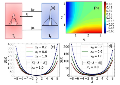
Figure 1: a) Schematic diagram of two squeezed harmonic baths interacting with two energy levels. b) Density plot of the thermodynamic affinity under equal temperature setting as per Eq.(18) with $\omega_{o}=0.5(\hbar=1,k_{B}=1),T_{L}=T_{R}=0.7$. In (c) (d) the GC symmetry is shown as per Eq.(17) with $T_{L}=0.7,T_{R}=0.4$. The solid (dotted) line represent $S(\lambda)(S(-\lambda-A))$. Throughout the numerics, we have used $\Gamma_{L}=\Gamma_{R}=1s^{-1}$.

The Hamiltonian of the two level system interacting with two bosonic reservoirs (Fig.(1)a) can be written as,

$$\hat{H} =\displaystyle\hbar\omega_{o}\hat{b}^{\dagger}\hat{b}+\sum_{i=\nu,\nu\in L,R}\hbar\omega_{i}\hat{a}_{i}^{\dagger}\hat{a}_{i}+\hat{V},$$ (1)

with

$$\hat{V} =\sum_{i,\nu\in L,R}k_{i}^{\nu}(\hat{a}_{i\nu}^{\dagger}\hat{b}+\hat{a}_{i\nu}\hat{b}^{\dagger})$$ (2)

Here, $\hbar\omega_{o}\hat{b}^{\dagger}\hat{b}$ is the on site Hamiltonian with bare frequency $\omega_{o}$, while $\hat{b}^{\dagger}(\hat{b})$ is the bosonic creation (annihilation operator) on the site. The second term is the reservoir Hamiltonian with squeezed harmonic states and is a sum of two terms that represent the left (L) and right (R) squeezed reservoirs. The single particle operators $\hat{a}_{i\nu}^{\dagger}(\hat{a}_{i\nu})$ represent the creation (annihilation) of a boson in the i-th mode from (of) the $\nu$-th bath. $\hat{V}$ is the system bath coupling Hamiltonian with $k_{i}^{\nu}$ being the coupling constant for the i-th squeezed mode of the $\nu$th bath to the bare site mode. The schematic representation of the model is shown in Fig.(1 a). The squeezed density matrix for the $\nu$-th reservoir ($\hat{H}_{\nu}$ being the $\nu$th reservoir Hamiltonian) is given by

$$\hat{\rho}_{\nu} =\frac{1}{Z}\exp\{-\beta_{\nu}\hat{S}\hat{H}_{\nu}\hat{S}^{\dagger}\},$$ (3)

with $\beta_{\nu}=(k_{B}T_{\nu})^{-1}$ being the inverse temperature and $\hat{S}$ is the squeezing operator on the $k-th$ bath mode given by :

$$\hat{S} =\displaystyle\prod_{k}e^{\frac{1}{2}(\lambda_{k\nu}^{*}\hat{a}_{k\nu}^{{\dagger}2}-h.c)},$$ (4)

$$\lambda_{k\nu} =x_{k\nu}e^{i\theta_{k\nu}},x_{k\nu}>0$$ (5)

with $x_{k\nu},\theta_{k\nu}$ being the squeezing parameters Dodonov (2002); Li et al. (2017); Yadalam et al. (2022).

We are interested in the statistics of boson transport between system, represented by the reduced density matrix $\hat{\rho}$ and the squeezed baths. We choose to count the net number of bosons exchanged with the left reservoir and denote it as $q$. To keep track of $q$, we can write down a moment generating vector for the reduced system within the FCS formalism Esposito et al. (2009); Harbola et al. (2007); Goswami and Harbola (2015). We formulate this in the Liouville space in terms of the auxiliary counting field, $\lambda$. The reduced moment generating density vector, $|\breve{\rho}(\lambda,t)\rangle\rangle$, can be written as,

$$|\dot{\breve{\rho}}(\lambda,t)\rangle\rangle={\breve{\cal L}}(\lambda)|\breve{\rho}(0,0)\rangle\rangle,$$ (6)

where the elements of the density vector contains the populations of the occupied and unoccupied states, $\{\rho_{11}$, $\rho_{00}\}$ (appendix) with the evolution superoperator, ${\breve{\cal L}}(\lambda)$, given by

$${\breve{\cal L}}(\lambda) =\left[\begin{array}[]{cc}-\alpha_{L}-\alpha_{R}&\beta_{L}e^{\lambda}+\beta_{R}\\ \alpha_{L}e^{-\lambda}+\alpha_{R}&-\beta_{L}-\beta_{R}\end{array}\right].$$ (9)

The rates of boson exchange between system and reservoirs are given by (we ignore the Lamb shifts terms):

$$\alpha_{\nu} =\Gamma_{\nu}(1+N_{\nu}),\nu=L,R$$ (10)

$$\beta_{\nu} =\Gamma_{\nu}N_{\nu}$$ (11)

with the occupation factor being

$$N_{\nu} =\cosh{(2x_{\nu})\bigg{(}n_{\nu}+\frac{1}{2}\bigg{)}-\frac{1}{2}}$$ (12)

where $n_{\nu}=(e^{\beta_{\nu}\hbar\omega_{o}}-1)^{-1}$ being the the Bose-Einstein distribution of the $\nu$-th bath. $x_{\nu}>0$ is the renormalized parameter responsible for squeezing the $\nu$-th harmonic bath within the Markovian regime Li et al. (2017) (see the appendix). In the steadystate, one of smaller eigenvalues of the RHS of Eq.(9), $S(\lambda)$ corresponds to a cumulant generating function, from which the cumulants of boson exchange can be directly evaluated as,

$$j^{(n)} =\partial_{\lambda}^{n}S(\lambda)|_{\lambda=0}.$$ (13)

Here, $n=1,2,3$ and $4$ corresponds to the flux, noise, skewness and kurtosis respectively, which we evaluate in the next section.

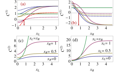
Figure 2: (Color online) Plots showing the behavior of the flux ($C^{(1)})$ and noise, ($C^{(2)})$) as a function of the squeezing parameters $x_{L}$ and $x_{R}$ with $n_{L}=1$ and $n_{R}=0.1$. In (a) and (b), the solid lines represent flux and the dotted lines represent $A$. The straight line at unity (green) is evaluated at $x_{L}=x_{R}$ and the other curves are evaluated at $x_{\nu}$ =1 (purple), 0.5(golden) and 0(blue). Both the quantities saturate at high squeezing values. The saturation value of A as a function of $x_{L}(x_{R})$ is dictated by Eq. (19(20)). The saturation value of $C^{(1)}$ as a function of $x_{\nu}$ is at $\Gamma_{\nu}\tilde{n}_{\nu}\cosh(2x_{\nu})/j^{(1)}_{o}$. The change in the direction of flux occurs at $x_{\nu}^{*},\nu=L,R$ (Eq.(24)) and is indicated by the downward pointing arrow. In (a), the red dotted curve represents $A$ evaluated for $x_{R}=0.5(n_{L}=n_{R})$. In subfigures, (c) and (d) the noise is seen to be always greater than unity and saturates at $\Gamma_{\nu}\tilde{n}_{\nu}/j^{(2)}_{o}.$

III Results and Discussion

We start our discussion by stating that, the analytical form of the cumulant generating function $S(\lambda)$ is given by

$$S(\lambda)= -(\alpha_{L}+\alpha_{R}+\beta_{L}+\beta_{R})$$ (14)

$$+\sqrt{(\alpha_{L}+\alpha_{R}+\beta_{L}+\beta_{R})^{2}+4f(\lambda)})$$ (15)

$$f(\lambda) =\alpha_{L}\beta_{R}(e^{-\lambda}-1)+\alpha_{R}\beta_{L}(e^{\lambda}-1)$$ (16)

and has the same mathematical structure as the one obtained from harmonic baths Agarwalla and Segal (2018); Ren et al. (2010), albeit with squeezed rates. Hence it satisfies a Gallavoti-Cohen (GC) symmetry

$$S(\lambda)=S(-\lambda-A)$$ (17)

with a squeezing dependent thermodynamic affinity, A, given by,

$$A=\log\left(\frac{(\tilde{n}_{L}\cosh(2x_{L})-1)(\tilde{n}_{R}\cosh(2x_{R})+1)}{(\tilde{n}_{L}\cosh(2x_{L})+1)(\tilde{n}_{R}\cosh(2x_{R})-1)}\right)$$ (18)

where we have defined $\tilde{n}_{\nu}=1+2n_{\nu}$. The GC symmetry ensures the validity of a steadystate FT of the type, $P(q)/P(-q)=\exp(qA)$. The validity of GC symmetry is graphically shown in Fig.(IIb,c) for various squeezing values. Note that, one recovers the standard expression of the affinity (we denote it as $A_{o}$), $A_{o}=\Delta\beta=(\hbar\omega_{o}/k_{B})(T_{L}^{-1}-T_{R}^{-1})/k_{B}$ when $x_{\nu}=0$. Note that, when $T_{L}=T_{R}$, the affinity goes to zero for the unsqueezed case (harmonic case) and indicates thermal equilibrium ($A_{o}=0$). However, for the squeezed case, maintaining $T_{L}=T_{R}$ in Eq.(18), we find that $A\neq 0$ as long as $x_{L}\neq x_{R}$. Thus by unsymmetrically squeezing the two reservoirs, one can kick the system out of equilibrium even when the temperatures are equal. We graphically show the nonzero value of A under the equal temperature setting in Fig.(IId) by varying both $x_{L}$ and $x_{R}$. This is graphically also shown in the dashed and dotted curve in Fig.(2a). In Fig.(2 a (b)) each of the dashed curves represent the thermodynamic affinity evaluated at different $x_{R}(x_{L})$ as a function of $x_{L}(x_{R})$. These curves saturate for high squeezing values. These saturation values are given by,

$$\lim_{x_{L}\to\infty}A =\log\frac{\tilde{n}_{R}\cosh(2x_{R})+1}{\tilde{n}_{R}\cosh(2x_{R})-1}$$ (19)

$$\lim_{x_{R}\to\infty}A =\log\frac{\tilde{n}_{L}\cosh(2x_{L})-1}{\tilde{n}_{L}\cosh(2x_{L})+1}.$$ (20)

The above two equations indicate that, only one value of the Bose-Einstein factor dominates in the high squeezing limit. Both the saturated values are finite and greater than zero even when $T_{L}=T_{R}(n_{L}=n_{R})$. The saturated values become zero if and only if $x_{L}=x_{R}$ as well as $n_{L}=n_{R}$.

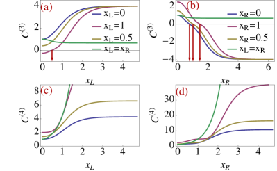
Figure 3: (Color online) Plots showing the behavior of the skewness ($C^{(3)})$ and kurtosis, ($C^{(4)})$) as a function of the squeezing parameters. In (a) and (b), the solid lines represent flux and the dotted lines represent $A$. The straight line at unity (green) is evaluated at $x_{L}=x_{R}$ and the other curves are evaluated at $x_{\nu}$ =1 (purple), 0.5(golden) and 0(blue). In subfigures, (c) and (d) the kurtosis is seen to be always greater than unity. Both cumulants saturate at the values predicted by Eqs.(31,30). Numerical parameters used are given in Fig.(2) and color-matched.

We can now proceed to evaluate the cumulants using Eqs.(9) and (13). Note that, one recovers the standard generating function for bosonic transport in absence of squeezing, $x_{\nu}=0$ in Eq.(9)Agarwalla and Segal (2018). We denote the cumulants in absence of squeezing as $j^{(n)}_{o}$ and define a dimensionless ratio representing the scaled cumulants,

$$C^{(n)}:=\displaystyle\frac{j^{(n)}}{j^{(n)}_{o}}$$ (21)

which signifies the extent of change in the values of the squeezed cumulants in comparison to unsqueezed case. When$|C^{(n)}|>(<)1$, the squeezing increases (decreases) the value of the cumulant in comparison to the unsqueezed case. We plot the dimensionless cumulant ratio $C^{(n)}$ as a function of squeezing parameters which are shown graphically in figures (2) and (3) for $n=1,2,3$ and $4$.

The first cumulant of flux can be be written as

$$j^{(1)} =\frac{\Gamma(\tilde{n}_{L}\cosh(2x_{L})-\tilde{n}_{R}\cosh(2x_{R}))}{\Gamma_{L}\tilde{n}_{L}\cosh(2x_{L})+\Gamma_{R}\tilde{n}_{R}\cosh(2x_{R})}$$ (22)

with $\Gamma=\Gamma_{L}\Gamma_{R}$. Under the symmetric squeezing case, $x_{L}=x_{R}$, the above equation reduces to the standard expression of flux in absence of squeezing,

$$j^{(1)}\big{|}_{x_{L}=x_{R}}=j^{(1)}_{o}=\frac{2\Gamma(n_{L}-n_{R})}{\Gamma_{L}\tilde{n}_{L}+\Gamma_{R}\tilde{n}_{R}},$$ (23)

From the above equation, it is evident that the flux is independent of squeezing when both the bosonic reservoirs are squeezed symmetrically. The quantity $C^{(1)}$ is graphically shown in Fig.(2a,b). The crossover from negative to positive flux happens since the thermodynamic affinity becomes negative (shown as dotted lines in Fig.(2a,b)). This switching of the direction of flux occurs at the point $x_{\nu}^{*}$

$$x_{\nu}^{*}=\frac{1}{2} \cosh^{-1}\left(\frac{\tilde{n}_{\nu}\cosh(2x_{\nu})}{\tilde{n}_{\nu}^{{}^{\prime}}}\right),\nu\neq\nu^{\prime}\in L,R$$ (24)

and shown graphically via downward arrow in Fig.(2a,b). Further, whenever $\cosh(2x_{L})>(<)\cosh(2x_{R})$, $C^{(1)}>(<)1,$ if $T_{L}\geq T_{R}$ is maintained.

The noise or second order cumulant can be expressed as,

$$j^{(2)} =\frac{\Gamma\left((\tilde{n}_{L}\tilde{n}_{R}\cosh(2x_{L})\cosh(2x_{R})-1)(\Gamma_{L}\tilde{n}_{L}\cosh(2x_{L})+\Gamma_{R}\tilde{n}_{R}\cosh(2x_{R}))^{2}-\Gamma(\tilde{n}_{L}\cosh(2x_{L})-\tilde{n}_{R}\cosh(2x_{R}))^{2}\right)}{(\Gamma_{L}\tilde{n}_{L}\cosh(2x_{L})+\Gamma_{R}\tilde{n}_{R}\cosh(2x_{R}))^{3}}$$ (25)

which under equal squeezing ($x_{L}=x_{R}$) can be recast as:

$$j^{(2)}|_{x_{L}\to x_{R}} =\frac{-\Gamma((\Gamma_{L}+\Gamma_{R})(\Gamma_{L}\tilde{n}_{L}^{2}+\Gamma_{R}\tilde{n}_{R}^{2})+\tilde{n}_{L}\tilde{n}_{R}(\Gamma_{L}\tilde{n}_{L}+\Gamma_{R}\tilde{n}_{R})^{2}\cosh^{2}(2x_{L}))\text{sech}(2x_{R})}{(\Gamma_{L}\tilde{n}_{L}+\Gamma_{R}\tilde{n}_{R})^{3}},$$ (26)

and reduces to the standard known expression for the second cumulant Saryal et al. (2019) only when, $x_{R}=x_{L}$=0,

$$j^{(2)}\big{|}_{x_{L},x_{R}=0} =j^{(2)}_{o}=\frac{2\Gamma(2n_{L}n_{R}+n_{L}+n_{R})}{\Gamma_{L}\tilde{n}_{L}+\Gamma_{R}\tilde{n}_{R}}-\frac{4\Gamma^{2}(n_{L}-n_{R})^{2}}{(\Gamma_{L}\tilde{n}_{L}+\Gamma_{R}\tilde{n}_{R})^{3}}$$ (27)

Note that under symmetric condition $x_{L}=x_{R}$, the RHS of Eq.(26) is not equal to the RHS of Eq.(27) indicating the dependence of noise under symmetric conditions unlike the flux (Eq.(23)). The quantity $C^{(2)}$ is shown graphically as a function of squeezing parameters in Fig.(2c,d). Note that, $C^{(2)}>1$ is maintained for all values of $x_{L},x_{R}>0$, indicating that squeezing always increases the magnitude of the noise. The skewness ($n=3$) can be expressed as (for compactness, we have used a shorthand notation, $\tilde{n}_{\nu}(x_{\nu}):=1+2n_{\nu}\cosh(2x_{\nu})$):

$$j^{(3)} =\displaystyle\frac{{\Gamma(\tilde{n}_{L}(x_{L})-\tilde{n}_{R}(x_{R}))\left(\Gamma_{L}^{4}\tilde{n}_{L}^{4}(x_{L})+\Gamma_{L}^{3}\Gamma_{R}\tilde{n}_{L}^{3}(x_{L})\tilde{n}_{R}^{3}(x_{L})+3\Gamma_{L}^{2}\Gamma_{R}(\Gamma_{L}+\Gamma_{R})\tilde{n}_{L}^{2}(x_{L})\atop+\frac{1}{2}\Gamma_{R}^{2}\tilde{n}_{R}^{2}(x_{R})\left(6\Gamma_{L}^{2}+6\Gamma+\Gamma_{R}^{2}\tilde{n}_{R}^{2}(2x_{R})+\Gamma_{R}^{2}\tilde{n}_{R}^{2}\right)+\Gamma_{L}\Gamma_{R}^{3}\tilde{n}_{L}(x_{L})\tilde{n}_{R}^{3}(x_{R})\right)}}{(\Gamma_{L}\tilde{n}_{L}(x_{L})+\Gamma_{R}\tilde{n}_{R}(x_{R}))^{5}}$$ (28)

which under the symmetric squeezing ($x_{L}=x_{R}$) is independent of squeezing and reduces to the standard resultSaryal et al. (2019),

$$j^{(3)}\big{|}_{x_{L}=x_{R}} =j^{(3)}_{o}=\frac{2\Gamma(n_{L}-n_{R})\left((\Gamma_{L}\tilde{n}_{L}+\Gamma_{R}\tilde{n}_{R})^{4}-6\Gamma(2n_{L}n_{R}+n_{L}+n_{R})(\Gamma_{L}\tilde{n}_{L}+\Gamma_{R}\tilde{n}_{R})^{2}+12\Gamma(n_{L}-n_{R})^{2}\right)}{(\Gamma_{L}\tilde{n}_{L}+\Gamma_{R}\tilde{n}_{R})^{5}}$$ (29)

The quantity $C^{(3)}$ is graphically shown as a function of squeezing parameters in Fig.(3a,b). Note that, similar to the flux, a switching in the sign of the scaled skewness is observed as one keeps increasing the squeezing. The behavior of switching of the skewness from negative to positive can be understood in a similar manner to that of the flux. The switching point is given by Eq.(24) and are indicated by the downward arrows in Fig.(3a,b). $C^{(3)}>(<)1$ as long as $\cosh(2x_{L})>(<)\cosh(2x_{R})$ if $n_{L}>(<)n_{R}$. We conclude that all odd cumulants are independent of squeezing when both the reservoirs are squeezed symmetrically. This is graphically shown in Fig.(4a,c) by numerically evaluating the odd cumulants. As can be seen from the figure, the dotted curves that represent $j^{(n)}_{o}$, overlap with the solid curves, $j^{(n)}$ for the cumulants $n=5,7,9$ and $11$. The even cumulants however depend on the squeezing under symmetric conditions. We also find that all the odd and the even cumulants saturate to two different unique values, $j_{\infty}$ as a function of either of the squeezing parameters. The value of odd cumulants under large squeezing values is given by,

$$\lim_{x_{\nu^{\prime}}\to\infty}j^{(n)}|_{n\in odd}=j_{\infty}^{odd}=\Gamma_{\nu}\tilde{n}_{\nu}\cosh(2x_{\nu}),\nu\neq\nu^{\prime}\in L,R,$$ (30)

while the even cumulants’ saturation value is obtained at

$$\lim_{x_{\nu^{\prime}}\to\infty}j^{(n)}|_{n\in even}=j_{\infty}^{even}=\Gamma_{\nu},\nu\neq\nu^{\prime}\in L,R,$$ (31)

These saturation values are highlighted in Fig.(4) for $n=2\ldots 12$. The saturation behavior are also visible in figures (2 and 3), albeit scaled as $j^{(n)}_{\infty}/j^{(n)}_{o}$. An application of this result is that, Eq.(31) together with Eq.(30) would allow experimental determination of the coupling values and the Bose- Einstein distribution by simply squeezing the system to a large extent.

In Fig.(4 b and d), we show the even cumulants ($n=2,\ldots 10$) as a function of squeezing parameters under the condition $T_{L}=T_{R}$ and $\Gamma_{L}=\Gamma_{R}$. Under this case, we find that the cumulants behave identically when $x_{\nu}$ is varied for a fixed $x_{\nu^{\prime}}$. We explain this by taking the analytical expression of the noise in the aforesaid limit which is given by,

$$j^{(2)}_{e} =j^{(2)}|_{\Gamma_{L}\to\Gamma_{R},n_{L}\to n_{R}}$$ (32)

$$=\displaystyle\frac{\Gamma_{L}\left(\tilde{n}_{R}^{2}\cosh^{3}(2x_{L})\cosh(2x_{R})+\tilde{n}_{R}^{2}\cosh(2x_{L})\cosh^{3}(2x_{R})\atop+2\cosh^{2}(2x_{L})\left(\tilde{n}_{R}^{2}\cosh^{2}(2x_{R})-1\right)-2\cosh^{2}(2x_{R})\right)}{\tilde{n}_{R}(\cosh(2x_{L})+\cosh(2x_{R}))^{3}}.$$

The above expression is symmetric with respect to the exchange of $x_{L}$ with $x_{R}$ and vice-versa and hence results in an equivalent dependence of the even cumulants on the squeezing parameters. Note that, the thermodynamic affinity, $A$, is however antisymmetric with respect to exchange of $x_{L}$ and $x_{R}$ under the symmetric condition, i.e, $A(x_{L};x_{R})=-A(x_{R};x_{L})$, as evident from Eq.(18).

We now focus on the thermodynamic uncertainty relationship given by $FA>2k_{B}$, $F$ being the Fano factor, which in our case is given by

$$F=\frac{j^{(2)}}{j^{(1)}}$$ (33)

When $k_{B}\to 1$, $FA>1$ is shown to be valid for Markovian dynamics in many systems. In our case, we numerically evaluate the quantity $FA$ as a function of $x_{L}$ and $x_{R}$ and show the results graphically in Figs.(5) and (6). We see that the inequality holds for the entire range of $x_{L}$ and $x_{R}$ for a wide range of $n_{L}$ and $n_{R}$ values. The robustness is because of the validity of the Gallavoti-Cohen symmetry that leads to a steady state fluctuation theorem. Further it has also been predicted in Saryal et al. (2019) that, TURs in bosonic transport holds because of the specific mathematical form of the cumulant generating function Saryal et al. (2019), which makes the internal dynamics of the bath oscillators irrelevant during transport statistics. Such is the case for our system in the Markovian regime, where the analytical expression for the squeezed $S(\lambda)$, Eq.(14) and has the same mathematical structure as the one in conventional thermal transport, and hence TUR holds.

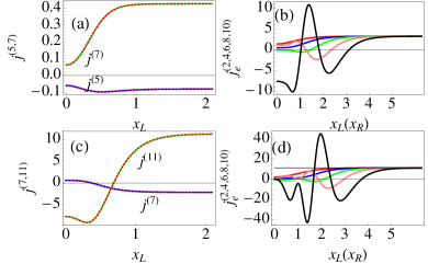
Figure 4: (Color Online) Behavior of higher odd and even cumulants. In (a) and (c), the values of odd cumulants are same for symmetric squeezing and unsqueezed case. These saturate to the scaled values given by Eq.30) In (b), $x_{\nu}=0.2$ and (d)$x_{\nu}=1$, the even cumulants are evaluated at $T_{L}=T_{R}$ which saturate at the values dictated by Eq.(31), indicated by straight line in (d). The red curves represent the analytical result from Eq.(32). The other curves are numerically evaluated for $n=4,6,8$ and 10 shown by the blue, green, pink and black curves, respectively.

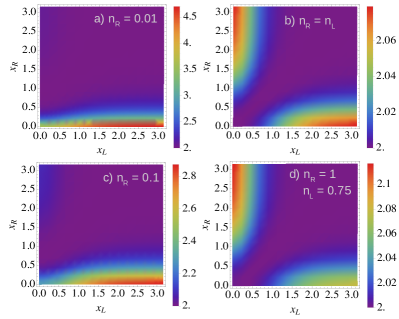
Figure 5: Density plots showing the robustness of the thermodynamic uncertainty relationship, $FA\geq 2$ as a function of the squeezing parameters, $x_{L}$ and $x_{R}$. Here $n_{L}=1$ and $n_{R}=0.1$ in a), b) and c).

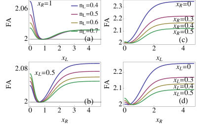
Figure 6: Behavior of the product $FA$ as a function of $x_{R}$ and $x_{R}$ for varying $n_{L}$ in (a), (b). $n_{L}=0.4,n_{R}=0.3$ is fixed in (c) and (d). $FA\geq 2$ holds for all the different conditions.

IV Conclusion

We theoretically explored the effect of squeezing on the flux and higher order fluctuations during boson exchange between two squeezed harmonic reservoirs and a two level system. Within the Markov approximation, we analytically showed that the direction of the steadystate flux can be reversed under appropriate squeezing conditions. The thermodynamic affinity is shown to be antisymmetric with respect to the interchange of the two squeezing parameters and is non zero when $T_{L}=T_{R}$. The odd cumulants are proven to be independent of squeezing when both the left and right reservoirs are squeezed symmetrically. The even cumulants however always depend on the two squeezing paramaters and are larger in magnitude in comparison to an unsqueezed case. Under high squeezing, the saturation values of the odd and even cumulants can be used to determine the coupling strength and Bose-Einstein distribution of the reservoirs, respectively since these cumulants saturate to two unique values. Under equal temperature setting, the even cumulants behave identically as a function of the squeezing parameters. A steady state fluctuation theorem is derived where the thermodynamic affinity is shown to be dependent on squeezing parameters. A thermodynamic uncertainty relationship holds in the presence of squeezing.

appendix

Upto second order in the perturbation of the coupling, $\hat{V}$, the reduced system dynamics is given by the Eq.(2):

$$\dot{\tilde{\rho}}=-tr_{B}\int_{o}^{t}ds(\rho_{T}(t)\tilde{V}(t)\tilde{V}(t_{s})-\tilde{V}(t)\tilde{\rho}_{T}(t)\tilde{V}(t_{s})+h.c)$$ (34)

with $t_{s}:=t-s$, in the interaction picture, $\tilde{O}(t)=\exp(i\hat{H}_{o}t)\hat{O}\exp(-i\hat{H_{o}}t)$. $\hat{H}_{o}$ contains only the diagonal part from Eq.(1). Assuming that the initial density matrix is factorisable, we can write $\tilde{\rho}_{T}:=\tilde{\rho}\otimes\rho_{B}$, with $\rho_{B}=\rho_{L}\otimes\rho_{R}$, being the squeezed density matrices for the left and right reservoirs respectively. Substituting the value of the operator $\hat{V}$ in Eq.(34), we can write the integrands as,

$$\tilde{\rho}\rho_{B}\tilde{V}_{s}\tilde{V} =k_{i\nu}^{2}\big{(}\langle\tilde{a}_{i\nu}^{\dagger}(t_{s})\tilde{a}_{i\nu}(t)\rangle\tilde{\rho}(\tilde{b}(t_{s})\tilde{b}(t)+\tilde{b}(t_{s})\tilde{b}^{\dagger}(t))$$ (35)

$$+\langle\tilde{a}_{i\nu}(t_{s})\tilde{a}_{i\nu}^{\dagger}(t)\rangle\tilde{\rho}(\tilde{b}(t_{s})\tilde{b}^{\dagger}(t)+\tilde{b}^{\dagger}(t_{s})b^{\dagger}(t))\big{)}$$

$$\tilde{V}\tilde{\rho}\rho_{B}\tilde{V}_{s} =k_{i\nu}^{2}\big{(}\langle\tilde{a}_{i\nu}^{\dagger}(t)\tilde{a}_{i\nu}(t_{s})\rangle(\tilde{b}(t)\tilde{\rho}\tilde{b}(t_{s})+\tilde{b}(t)\tilde{\rho}\tilde{b}^{\dagger}(t))$$ (36)

$$+\langle\tilde{a}_{i\nu}(t)\tilde{a}_{i\nu}^{\dagger}(t_{s})\rangle(\tilde{b}(t)\tilde{\rho}\tilde{b}^{\dagger}(t_{s})+\tilde{b}^{\dagger}(t)\tilde{\rho}b^{\dagger}(t_{s}))\big{)}$$

where $\langle.\rangle$ represents trace over the squeezed density matrix. On evaluating the matrix elements of Eq.(35) and (36), $\langle m|.|n\rangle,m,n=1,0$, only the terms with conjugate system operators survive leading to only $m=n$ terms. The nonzero squeezed bath expectation values are given by Li et al. (2017),

$$\langle\tilde{a}_{i\nu}^{\dagger}\tilde{a}_{i\nu}\rangle =\big{(}\cosh(2x_{i\nu})(n_{\nu}+\frac{1}{2})-\frac{1}{2}\big{)}f(t,s)$$ (37)

$$:=N_{\nu}f(t,s)$$ (38)

$$\langle\tilde{a}_{i\nu}\tilde{a}_{i\nu}^{{\dagger}}\rangle =\big{(}\cosh(2x_{i\nu})(n_{\nu}+\frac{1}{2})+\frac{1}{2}\big{)}f(t,s)$$ (39)

$$:=(1+N_{\nu})f(t,s)$$ (40)

where $n_{\nu}$ is the Bose function for the $\nu$-th squeezed bath and $f(t,s)=\exp(it_{s}\omega_{i\nu})\exp(-it\omega_{i\nu})$. With these definitions, a standard Born-Markov approximation ($t\to\infty$) within the wide-band limit we can evaluate the time integrands in Eq.(35) and (36) by substituting in Eq.(34). The wide band limit normalizes the squeezing parameter of the $k$th mode of the $\nu$th bath, $x_{i\nu}$ to a real positive number $x_{\nu}$ Li et al. (2017). We can now write down two coupled Pauli type master equations with squeezed rates given by,

$$\dot{\rho}_{11} =-(\Gamma_{L}(1+N_{L})+\Gamma_{R}(1+N_{R}))\rho_{11}$$ (41)

$$+(\Gamma_{L}N_{L}+\Gamma_{R}N_{R})\rho_{00}$$

$$\dot{\rho_{22}} =(\Gamma_{L}(1+N_{L})+\Gamma_{R}(1+N_{R}))\rho_{11}$$ (42)

$$-(\Gamma_{L}N_{L}+\Gamma_{R}N_{R})\rho_{00}$$

where $\langle m|\rho|m\rangle=\rho_{mm}$ represent the probability of occupation of the occupied and unoccupied states. Redefining the rates as $\alpha_{\nu}=\Gamma_{L}(1+N_{L})$ and $\beta_{\nu}=\Gamma_{\nu}N_{\nu}$, we can write the above two equations in the Liouville space as,

$$|\dot{\rho}\rangle\rangle ={\breve{\cal L}}|\rho\rangle\rangle$$ (43)

with the superoperator given by,

$$\breve{\cal L}=\left[\begin{array}[]{cc}-\alpha_{L}-\alpha_{R}&\beta_{L}+\beta_{R}\\ \alpha_{L}+\alpha_{R}&-\beta_{L}-\beta_{R}\end{array}\right]$$ (46)

Now following the standard procedure of FCS by introducing the auxiliary counting field, $\lambda$ to keep track of the net number of bosons exchanged, $1$ Esposito et al. (2009); Harbola et al. (2007); Goswami and Harbola (2015), we can arrive at Eq.(6).

References

- Walls (1983) D. F. Walls, nature 306, 141 (1983).
- Schnabel (2017) R. Schnabel, Physics Reports 684, 1 (2017).
- Dodonov et al. (1991) V. Dodonov, A. Klimov, and V. Man’ko, in Group Theoretical Methods in Physics (Springer, 1991) pp. 450–456.
- Puri (1997) R. Puri, pramana 48, 787 (1997).
- Slusher et al. (1985) R. Slusher, L. Hollberg, B. Yurke, J. Mertz, and J. Valley, Physical review letters 55, 2409 (1985).
- Carmichael and Orozco (2011) H. Carmichael and L. Orozco, Nature 474, 584 (2011).
- Ourjoumtsev et al. (2011) A. Ourjoumtsev, A. Kubanek, M. Koch, C. Sames, P. W. Pinkse, G. Rempe, and K. Murr, Nature 474, 623 (2011).
- Mehmet et al. (2010) M. Mehmet, H. Vahlbruch, N. Lastzka, K. Danzmann, and R. Schnabel, Physical Review A 81, 013814 (2010).
- Dodonov (2002) V. Dodonov, Journal of Optics B: Quantum and Semiclassical Optics 4, R1 (2002).
- Lütkenhaus et al. (1998) N. Lütkenhaus, J. Cirac, and P. Zoller, Physical Review A 57, 548 (1998).
- Banerjee and Srikanth (2008) S. Banerjee and R. Srikanth, The European Physical Journal D 46, 335 (2008).
- Manzano et al. (2016) G. Manzano, F. Galve, R. Zambrini, and J. M. Parrondo, Physical Review E 93, 052120 (2016).
- Li et al. (2017) S.-W. Li et al., Physical Review E 96, 012139 (2017).
- You and Li (2018) Y.-N. You and S.-W. Li, Physical Review A 97, 012114 (2018).
- Jahromi (2020) H. R. Jahromi, Physica Scripta 95, 035107 (2020).
- Macchiavello et al. (2020) C. Macchiavello, A. Riccardi, and M. F. Sacchi, Physical Review A 101, 062326 (2020).
- Zou et al. (2022) C.-J. Zou, Y. Li, J.-B. You, Q. Chen, W.-L. Yang, and M. Feng, arXiv preprint arXiv:2204.08260 (2022).
- Niedenzu et al. (2016) W. Niedenzu, D. Gelbwaser-Klimovsky, A. G. Kofman, and G. Kurizki, New Journal of Physics 18, 083012 (2016).
- Agarwalla et al. (2017) B. K. Agarwalla, J.-H. Jiang, and D. Segal, Physical Review B 96, 104304 (2017).
- Klaers et al. (2017) J. Klaers, S. Faelt, A. Imamoglu, and E. Togan, Physical Review X 7, 031044 (2017).
- Newman et al. (2017) D. Newman, F. Mintert, and A. Nazir, Physical Review E 95, 032139 (2017).
- Wang et al. (2021) C. Wang, H. Chen, and J.-Q. Liao, Physical Review A 104, 033701 (2021).
- Hsiang and Hu (2021a) J.-T. Hsiang and B.-L. Hu, Physical Review D 103, 065001 (2021a).
- Horowitz and Gingrich (2020) J. M. Horowitz and T. R. Gingrich, Nature Physics 16, 15 (2020).
- Agarwalla and Segal (2018) B. K. Agarwalla and D. Segal, Phys. Rev. B 98, 155438 (2018).
- Pietzonka et al. (2017) P. Pietzonka, F. Ritort, and U. Seifert, Physical Review E 96, 012101 (2017).
- Perarnau-Llobet (2019) M. Perarnau-Llobet, Quantum Views 3, 13 (2019).
- Hernández-Gómez et al. (2021) S. Hernández-Gómez, N. Staudenmaier, M. Campisi, and N. Fabbri, New Journal of Physics 23, 065004 (2021).
- Holmes et al. (2019) Z. Holmes, S. Weidt, D. Jennings, J. Anders, and F. Mintert, Quantum 3, 124 (2019).
- Yadalam et al. (2022) H. K. Yadalam, B. K. Agarwalla, and U. Harbola, arXiv preprint arXiv:2202.04011 (2022).
- Huang et al. (2012) X. Huang, T. Wang, X. Yi, et al., Physical Review E 86, 051105 (2012).
- Hsiang and Hu (2021b) J.-T. Hsiang and B.-L. Hu, Annals of Physics 433, 168594 (2021b).
- Talkner et al. (2013) P. Talkner, M. Morillo, J. Yi, and P. Hänggi, New Journal of Physics 15, 095001 (2013).
- Chen et al. (2022) X.-M. Chen, Z.-K. Chen, H.-X. Che, and C. Wang, Journal of Physics B: Atomic, Molecular and Optical Physics 55, 115502 (2022).
- Giraldi and Petruccione (2014) F. Giraldi and F. Petruccione, The European Physical Journal D 68, 1 (2014).
- Ren et al. (2010) J. Ren, P. Hänggi, and B. Li, Phys. Rev. Lett. 104, 170601 (2010).
- Pekola and Karimi (2021) J. P. Pekola and B. Karimi, Reviews of Modern Physics 93, 041001 (2021).
- Saito and Dhar (2007) K. Saito and A. Dhar, Physical Review Letters 99, 180601 (2007).
- Hertz (1910) P. Hertz, Annalen der Physik 33, 225 (1910).
- Esposito et al. (2009) M. Esposito, U. Harbola, and S. Mukamel, Reviews of modern physics 81, 1665 (2009).
- Harbola et al. (2007) U. Harbola, M. Esposito, and S. Mukamel, Physical Review B 76, 085408 (2007).
- Goswami and Harbola (2015) H. P. Goswami and U. Harbola, The Journal of Chemical Physics 142, 084106 (2015).
- Saryal et al. (2019) S. Saryal, H. M. Friedman, D. Segal, and B. K. Agarwalla, Physical Review E 100, 042101 (2019).