Broadband microwave detection using electron spins in a hybrid diamond-magnet sensor chip
Lorentzweg 1, 2628 CJ Delft, The Netherlands.
2Advanced institute for Materials Research (WPI-AIMR), Tohoku University; Sendai 980-8577, Japan.
3Kavli Institute for Theoretical Sciences, University of Chinese Academy of Sciences; Beijing 100190, China.
∗Corresponding author. Email: T.vanderSar@tudelft.nl )
Abstract
Quantum sensing has developed into a main branch of quantum science and technology. It aims at measuring physical quantities with high resolution, sensitivity, and dynamic range. Electron spins in diamond are powerful magnetic field sensors, but their sensitivity in the microwave regime is limited to a narrow band around their resonance frequency. Here, we realize broadband microwave detection using spins in diamond interfaced with a thin-film magnet. A pump field locally converts target microwave signals to the sensor-spin frequency via the non-linear spin-wave dynamics of the magnet. Two complementary conversion protocols enable sensing and high-fidelity spin control over a gigahertz bandwidth, allowing characterization of the spin-wave band at multiple gigahertz above the sensor-spin frequency. The pump-tunable, hybrid diamond-magnet sensor chip opens the way for spin-based sensing in the 100-gigahertz regime at small magnetic bias fields.
tocsectionMain TextElectron spins associated with nitrogen-vacancy (NV) defects in diamond are magnetic field sensors that provide high spatial resolution and sensitivity at room temperature [1, 2]. They have been used to study nuclear magnetic resonance at the nanoscale [3, 4], bio- [5], paleo- [6], and solid-state magnetism [7], and electric currents in quantum materials [8, 9]. Most of these applications focus on detecting magnetic fields in the 0-100 megahertz (MHz) frequency range, in which a toolbox of spin-control techniques enables high sensitivity and a tunable detection frequency without requiring a specific electron spin resonance (ESR) frequency [1]. In contrast, NV-based sensing in the microwave regime [1-100 gigahertz (GHz)] currently relies on tuning the ESR to the frequency of interest using a magnetic bias field [10]. This bias field changes the properties of e.g. magnetic or superconducting samples under study [33, 12], for instance by altering their excitation spectrum, which limits its application in materials science. Furthermore, the field must be on the Tesla scale for operation in the 10-100 GHz range [13], making the required magnets large and slow to adjust, precluding the small sensor packaging desired for technological applications.
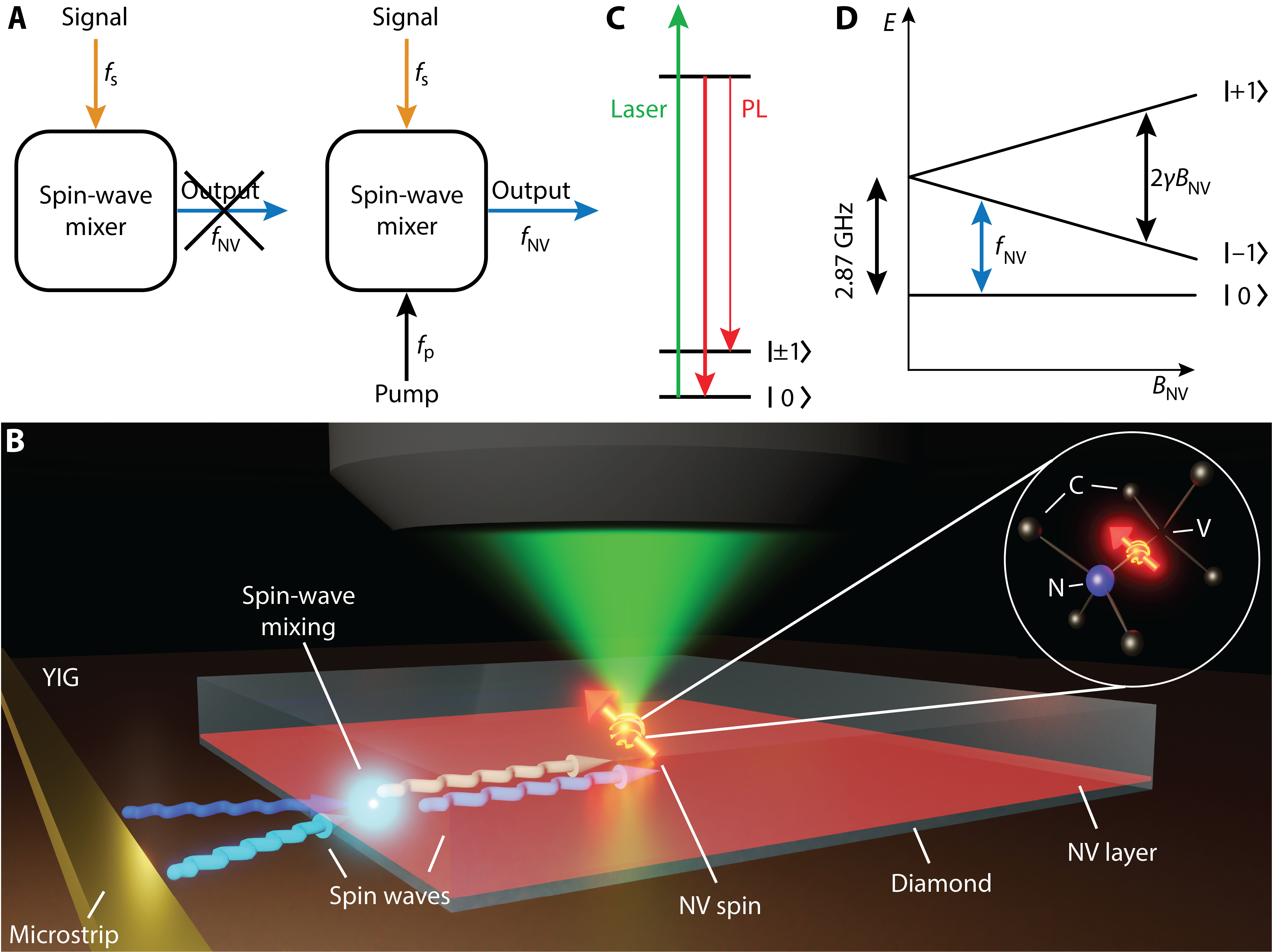
Here, we enable broadband spin-based microwave sensing by interfacing a diamond chip containing a layer of NV sensor spins with a thin-film magnet. The central concept is that the non-linear dynamics of spin waves - the collective spin excitations of the magnetic film [14] - locally convert a target signal to the NV ESR frequency under the application of a pump field (Fig. 1A-B). We realize a 1-GHz detection bandwidth at fixed magnetic bias field via four-spin-wave mixing, and microwave detection at multiple GHz above the ESR frequency via difference-frequency generation. The pump-tunable detection frequency enables characterizing the spin-wave band structure despite a multi-GHz detuning and provides insight into the non-linear spin-wave dynamics limiting the conversion process. Furthermore, the converted microwaves are highly coherent, enabling high-fidelity control of the sensor spins via off-resonant drive fields.
Our hybrid diamond-magnet sensor platform consists of an ensemble of near-surface NV spins in a diamond membrane positioned onto a thin film of yttrium iron garnet (YIG) - a magnetic insulator with low spin-wave damping [14] (Fig. 1B). A stripline delivers the “two-color” signal and pump microwave fields to the YIG film, in which they excite spin waves at the signal and pump frequencies, and , respectively. The frequency-converted microwaves at the ESR frequency are detected by measuring the spin-dependent NV photoluminescence under green laser excitation (Methods and Fig. 1C). The ESR frequency is fixed by an external magnetic bias field (Fig. 1D).
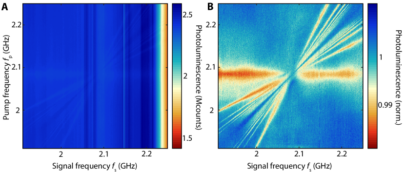
Our first detection protocol harnesses degenerate four-spin-wave mixing [15, 16, 17] - the magnetic analogue of optical four-wave mixing (Fig. 2A). In the quasiparticle picture, this process corresponds to the scattering of two “pump” magnons into a “signal” magnon and an “idler” magnon at frequency . This conversion enables the detection of a microwave signal that is detuned from the ESR frequency, which would be otherwise invisible in the optical response of the NV centers (Fig. 2B). By tuning the frequency of the pump, we enable the detection of signals of specific microwave frequencies (Fig. 2C).
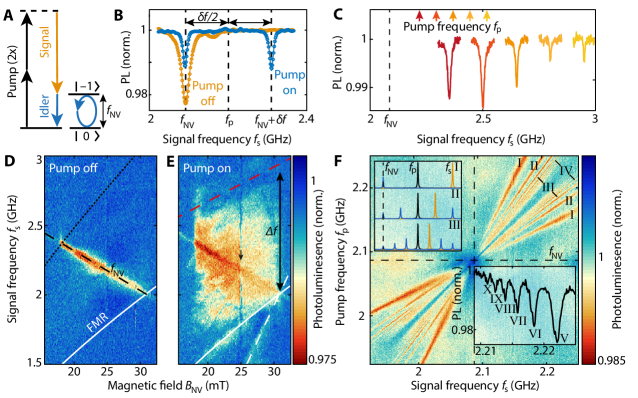
We characterize the bandwidth of the four-wave-mixing detection scheme by measuring the NV photoluminescence contrast as a function of the microwave signal frequency and magnetic bias field. As in Fig. 2B, when the pump field is switched off, we only detect signals resonant with (Fig. 2D). In contrast, when the pump is switched on, a broad band of frequencies becomes detectable (Fig. 2E). The bandwidth of 1 GHz is limited from below by the ferromagnetic resonance (FMR), the spatially homogenous spin-wave mode below which spin waves cannot be excited in our measurement geometry, and from above by the limited efficiency of our 5-micron-wide stripline to excite high-momentum spin waves. As such, the bandwidth can be extended by using narrower striplines or magnetic coplanar waveguides [19].
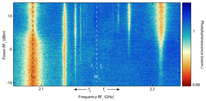
At 14 dBm signal and pump power, consecutive mixing processes generate higher-order idler modes at discrete and equally spaced frequencies (Fig. 2F). Motivated by the success of their optical counterparts in high-precision spectrometry [20], such “spin-wave frequency combs” are of great interest because of potential applications in microwave metrology [21, 22, 23]. We use the spin-wave comb to realize sensitivity to multiple microwave frequencies by detecting the n-th order idler frequency,
| (1) |
when it is resonant with the ESR frequency (Fig. 2F, upper inset). An increasing number of idler modes appears with increasing drive power (Fig. S3), such that at large powers we resolve up to the idler order (Fig. 2F, bottom inset). The shift of the idler frequency is amplified by the integer over the shift of the signal frequency (Eq. 1), leading to a decrease in the linewidth of the NV ESR response [22] (Fig. 2F) and a correspondingly enhanced ability to resolve closely spaced signal frequencies.
In addition to enabling off-resonant quantum sensing, the idlers also provide a resource for off-resonant control of spin- or other quantum systems. The resolving of the NV’s 3-MHz hyperfine splitting in the idler-driven ESR spectrum (Fig. 3A) evidences the high coherence of the microwave field emitted by the idler spin wave, implying that the linewidth is determined by the drive rather than the spin-wave damping [22]. This allows driving coherent NV spin rotations (Rabi oscillations) by pulsing the pump with varying duration (Fig. 3B).
Remarkably, these Rabi oscillations respond to externally applied microwaves that are detuned by hundreds of MHz from the ESR frequency (Fig. 3C). Such magnon-mediated, off-resonant Rabi control is a new instrument in the toolbox of spin-manipulation techniques, providing universal off-resonant quantum control with potential applications in quantum information processing. The idler-driven Rabi frequency exceeds the signal-induced AC Stark shift [34] by about an order of magnitude for the same off-resonant signal power (Fig. S4). The decrease of the Rabi frequency with increasing detuning (Fig. 3C) is attributed to a reduced spin-wave excitation efficiency at higher frequency and a reduced frequency-conversion efficiency due to an increased momentum mismatch between signal and pump spin waves [17].
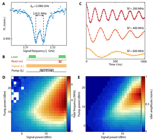
Since the Rabi frequency depends linearly on the idler amplitude [33], it provides insight into the magnetization dynamics in the film. As expected, the idler amplitude initially grows with increasing signal and pump power [15, 23], but then reaches a maximum and starts to decrease (Fig. 3D). We attribute the decrease to Suhl instabilities of the second type [16]: Both signal and pump modes decay into a pair of high-momentum magnons beyond a certain threshold amplitude, which drains energy from the idler mode. This interpretation is supported by a model of the four-wave interactions between the dominant two idler modes, the signal and pump modes, and the two pairs of high-momentum “Suhl” magnons (Figs. S5 and S6). The intermode coupling is induced by exchange and dipolar interactions, as well as crystalline anisotropy, and follows from the leading-order terms in the Holstein-Primakoff expansion [36]. Based on the interacting eight-mode Hamiltonian we compute the steady-state dynamics of the idler mode as a function of pump and signal power (Fig. 3E), which qualitatively reproduces the observed power dependence in Fig. 3D. Nanopatterning the magnetic film into a magnonic crystal modulates the magnon density of states, which may suppress the decay into unwanted spin-wave modes [14, 26] and thereby enable higher idler-driven Rabi frequencies.
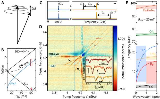
Our second detection protocol relies on difference-frequency generation, which enables down-conversion of GHz signals to MHz frequencies accessible to established quantum sensing techniques [1]. The difference frequency is generated by the longitudinal component of the magnetization under the driving of two spin waves of different frequencies [27]. In contrast to the four-wave mixing protocol, the converted frequency does not have to lie within the spin-wave band. By tuning the ESR frequency into resonance with the difference frequency (Fig. 4B), we detect microwave signals that are detuned by several gigahertz when (Fig. 4C). Alternatively, AC magnetometry protocols can provide difference-frequency detection with enhanced sensitivity at arbitrary bias [1]. We only observe ESR contrast when both and are above the FMR (Fig. 4D), confirming that the conversion is mediated by spin waves. As such, the efficiency of the conversion process can be used to characterize high-frequency magnetic band structures. Similar to Fig. 2E, the conversion is limited by the spin-wave excitation efficiency, which explains the observation of the largest ESR contrast for long-wavelength spin waves (i.e. just above the FMR).
We demonstrated magnon-mediated, spin-based sensing of microwave magnetic fields over a gigahertz bandwidth at a fixed magnetic bias field. The frequency of the pump determines the detection frequency, and the detection range is set by the frequencies at which spin waves can be excited efficiently. The range could be extended to the 10-100 GHz scale using materials with a larger magnetization that increases the spin-wave group velocity or crystal anisotropies that increase the spin-wave gap (Fig. 4E). The coherent nature of the frequency conversion allows combining with advanced spin-manipulation protocols such as heterodyne or dressed-state sensing [28, 29, 30] to further increase the detection capabilities. Wide-field readout of NV centers in a larger sensing volume would enhance the sensitivity, which is ultimately limited by thermally generated spin-wave noise. The demonstrated hybrid diamond-magnet sensor platform enables broadband microwave characterization without requiring large magnetic bias fields and opens the way for probing high-frequency magnetic spectra of new materials, such as van-der-Waals magnets.
Methods
Experimental setup. The NV photoluminescence is read out using a confocal microscope described in Ref. [33]. The NV-YIG chip and its fabrication were described in Ref. [31]. It consists of a 2x2x0.05-mm3 diamond membrane with an estimated near-surface NV density of placed on top of a 235-nm-thick YIG film grown using liquid phase epitaxy on a 500-m-thick GGG substrate (Matesy GmbH). The diamond-YIG separation distance is 2 m, limited by small particles (such as dust) between the diamond and the YIG surfaces. The signal and pump microwaves are generated by two Rohde Schwarz microwave sources (SGS100A), combined by a Mini-Circuits power combiner (ZFRSC-123-S+, total loss: -10 dB) and amplified by an AR amplifier (30S1G6, amplification: 44 dB). All measurements were performed at room temperature.
NV microwave magnetometry. The four NV-center families are sensitive to microwave magnetic fields at their electron spin resonance (ESR) frequencies, which are determined by the magnetic bias field via the NV spin Hamiltonian , with the zero-field splitting, the electron gyromagnetic ratio and the th spin-1 Pauli matrix. In this work, we align the field along one of the NV orientations, such that this “on-axis” family has ESR frequencies given by (with ). For the other three “off-axis” families, the bias field is equally misaligned by due to crystal symmetry, leading to the ESR frequency plotted in Fig. 4B (labeled “Off-axis”). The photoluminescence dips were recorded using continuous-wave microwaves and non-resonant optical excitation at 515 nm. For the Rabi oscillations we first initialize the NV spin in the -state via a 1-s green laser pulse, then we drive the spin using an idler pulse and finally we read out the NV photons in the first 300-400 ns of a second laser pulse.
Data processing. The data presented in Figs. 2F and 4D is normalized by the median of each row and column (Fig. S2).
References
- [1] C.. Degen, F. Reinhard and P. Cappellaro “Quantum sensing” In Reviews of Modern Physics 89.3, 2017, pp. 035002 DOI: 10.1103/RevModPhys.89.035002
- [2] L Rondin et al. “Magnetometry with nitrogen-vacancy defects in diamond” In Reports on Progress in Physics 77.5, 2014, pp. 056503 DOI: 10.1088/0034-4885/77/5/056503
- [3] Nabeel Aslam et al. “Nanoscale nuclear magnetic resonance with chemical resolution” In Science 357.6346, 2017, pp. 67–71 DOI: 10.1126/science.aam8697
- [4] I. Lovchinsky et al. “Magnetic resonance spectroscopy of an atomically thin material using a single-spin qubit” In Science 355.6324, 2017, pp. 503–507 DOI: 10.1126/science.aal2538
- [5] Romana Schirhagl, Kevin Chang, Michael Loretz and Christian L. Degen “Nitrogen-Vacancy Centers in Diamond: Nanoscale Sensors for Physics and Biology” In Annual Review of Physical Chemistry 65.1 Annual Reviews Inc., 2014, pp. 83–105 DOI: 10.1146/annurev-physchem-040513-103659
- [6] D.. Glenn et al. “Micrometer‐scale magnetic imaging of geological samples using a quantum diamond microscope” In Geochemistry, Geophysics, Geosystems 18.8, 2017, pp. 3254–3267 DOI: 10.1002/2017GC006946
- [7] Francesco Casola, Toeno Sar and Amir Yacoby “Probing condensed matter physics with magnetometry based on nitrogen-vacancy centres in diamond” In Nature Reviews Materials 3 Macmillan Publishers Limited, 2018, pp. 17088 URL: http://dx.doi.org/10.1038/natrevmats.2017.88%20http://10.0.4.14/natrevmats.2017.88
- [8] Mark J.. Ku et al. “Imaging viscous flow of the Dirac fluid in graphene” In Nature 583.7817, 2020, pp. 537–541 DOI: 10.1038/s41586-020-2507-2
- [9] J.-P Tetienne et al. “Quantum imaging of current flow in graphene” In Science Advances 3.e1602429, 2017
- [10] Patrick Appel, Marc Ganzhorn, Elke Neu and Patrick Maletinsky “Nanoscale microwave imaging with a single electron spin in diamond” In New Journal of Physics 17.11 IOP Publishing, 2015
- [11] Iacopo Bertelli et al. “Magnetic resonance imaging of spin-wave transport and interference in a magnetic insulator” In Science Advances 6.46, 2020, pp. eabd3556 DOI: 10.1126/sciadv.abd3556
- [12] L. Thiel et al. “Quantitative nanoscale vortex imaging using a cryogenic quantum magnetometer” In Nature Nanotechnology 11.8, 2016, pp. 677–681 DOI: 10.1038/nnano.2016.63
- [13] Benjamin Fortman et al. “Electron–electron double resonance detected NMR spectroscopy using ensemble NV centers at 230 GHz and 8.3 T” In Journal of Applied Physics 130.8, 2021, pp. 083901 DOI: 10.1063/5.0055642
- [14] A.. Chumak, V.. Vasyuchka, A.. Serga and B. Hillebrands “Magnon spintronics” In Nature Physics 11.6, 2015, pp. 453–461 DOI: 10.1038/nphys3347
- [15] J. Marsh and R.. Camley “Two-wave mixing in nonlinear magnetization dynamics: A perturbation expansion of the Landau-Lifshitz-Gilbert equation” In Physical Review B 86.22, 2012, pp. 224405 DOI: 10.1103/PhysRevB.86.224405
- [16] H. Suhl “The theory of ferromagnetic resonance at high signal powers” In Journal of Physics and Chemistry of Solids 1.4, 1957, pp. 209–227 DOI: 10.1016/0022-3697(57)90010-0
- [17] H. Schultheiss, K. Vogt and B. Hillebrands “Direct observation of nonlinear four-magnon scattering in spin-wave microconduits” In Physical Review B 86.5, 2012, pp. 054414 DOI: 10.1103/PhysRevB.86.054414
- [18] Iacopo Bertelli et al. “Imaging Spin‐Wave Damping Underneath Metals Using Electron Spins in Diamond” In Advanced Quantum Technologies 4.12, 2021, pp. 2100094 DOI: 10.1002/qute.202100094
- [19] Ping Che et al. “Efficient wavelength conversion of exchange magnons below 100 nm by magnetic coplanar waveguides” In Nature Communications 11.1, 2020, pp. 1445 DOI: 10.1038/s41467-020-15265-1
- [20] Nathalie Picqué and Theodor W. Hänsch “Frequency comb spectroscopy” In Nature Photonics 13.3, 2019, pp. 146–157 DOI: 10.1038/s41566-018-0347-5
- [21] Zhenyu Wang et al. “Magnonic Frequency Comb through Nonlinear Magnon-Skyrmion Scattering” In Physical Review Letters 127.3, 2021, pp. 037202 DOI: 10.1103/PhysRevLett.127.037202
- [22] Chris Koerner et al. “Frequency multiplication by collective nanoscale spin-wave dynamics” In Science 375.6585, 2022, pp. 1165–1169 DOI: 10.1126/science.abm6044
- [23] Tobias Hula et al. “Spin-wave frequency combs”, 2021 arXiv: http://arxiv.org/abs/2104.11491
- [24] Changjiang Wei, Andrew S M Windsor and Neil B Manson “A strongly driven two-level atom revisited: Bloch - Siegert shift versus dynamic Stark splitting” In Journal of Physics B: Atomic, Molecular and Optical Physics 30.21, 1997, pp. 4877–4888 DOI: 10.1088/0953-4075/30/21/022
- [25] Pavol Krivosik and Carl E. Patton “Hamiltonian formulation of nonlinear spin-wave dynamics: Theory and applications” In Physical Review B 82.18, 2010, pp. 184428 DOI: 10.1103/PhysRevB.82.184428
- [26] Y. Li et al. “Nutation Spectroscopy of a Nanomagnet Driven into Deeply Nonlinear Ferromagnetic Resonance” In Physical Review X 9.4, 2019, pp. 041036 DOI: 10.1103/PhysRevX.9.041036
- [27] B Flebus and Y Tserkovnyak “Quantum-Impurity Relaxometry of Magnetization Dynamics” In Physical Review Letters 121.18 American Physical Society, 2018, pp. 187204 DOI: 10.1103/PhysRevLett.121.187204
- [28] Jonas Meinel et al. “Heterodyne sensing of microwaves with a quantum sensor” In Nature Communications 12.1, 2021, pp. 2737 DOI: 10.1038/s41467-021-22714-y
- [29] T. Joas, A.. Waeber, G. Braunbeck and F. Reinhard “Quantum sensing of weak radio-frequency signals by pulsed Mollow absorption spectroscopy” In Nature Communications 8.1, 2017, pp. 964 DOI: 10.1038/s41467-017-01158-3
- [30] Alexander Stark et al. “Narrow-bandwidth sensing of high-frequency fields with continuous dynamical decoupling” In Nature Communications 8.1, 2017, pp. 1105 DOI: 10.1038/s41467-017-01159-2
References
- [31] Iacopo Bertelli et al. “Imaging Spin‐Wave Damping Underneath Metals Using Electron Spins in Diamond” In Advanced Quantum Technologies 4.12, 2021, pp. 2100094 DOI: 10.1002/qute.202100094
- [32] Avinash Rustagi, Iacopo Bertelli, Toeno Sar and Pramey Upadhyaya “Sensing chiral magnetic noise via quantum impurity relaxometry” In Physical Review B 102.22, 2020, pp. 220403 DOI: 10.1103/PhysRevB.102.220403
- [33] Iacopo Bertelli et al. “Magnetic resonance imaging of spin-wave transport and interference in a magnetic insulator” In Science Advances 6.46, 2020, pp. eabd3556 DOI: 10.1126/sciadv.abd3556
- [34] Changjiang Wei, Andrew S M Windsor and Neil B Manson “A strongly driven two-level atom revisited: Bloch - Siegert shift versus dynamic Stark splitting” In Journal of Physics B: Atomic, Molecular and Optical Physics 30.21, 1997, pp. 4877–4888 DOI: 10.1088/0953-4075/30/21/022
- [35] Mehrdad Elyasi, Eiji Saitoh and Gerrit E.. Bauer “Stochasticity of the magnon parametron” In Physical Review B 105.5, 2022, pp. 054403 DOI: 10.1103/PhysRevB.105.054403
- [36] Pavol Krivosik and Carl E. Patton “Hamiltonian formulation of nonlinear spin-wave dynamics: Theory and applications” In Physical Review B 82.18, 2010, pp. 184428 DOI: 10.1103/PhysRevB.82.184428
- [37] Xi Shen et al. “Multi-domain ferromagnetic resonance in magnetic van der Waals crystals CrI3 and CrBr3” In Journal of Magnetism and Magnetic Materials 528, 2021, pp. 167772 DOI: 10.1016/j.jmmm.2021.167772
- [38] N. León-Brito et al. “Magnetic microstructure and magnetic properties of uniaxial itinerant ferromagnet Fe3GeTe2” In Journal of Applied Physics 120.8, 2016, pp. 083903 DOI: 10.1063/1.4961592
Acknowledgments
We thank M. N. Ali for reviewing the manuscript. This work was supported by the Dutch Research Council (NWO) through the Frontiers of Nanoscience (NanoFront) program, the NWO Projectruimte grant 680.91.115, the Kavli Institute of Nanoscience Delft, and the Japan Society for the Promotion of Science (JSPS) by Kakenhi Grant 19H00645.
Author contributions. J.J.C. and T.v.d.S. conceived the experiment. I.B. built the setup and fabricated the sample. R.W.M., J.J.C., I.B. and A.T. performed the measurements and analyzed the data. M.E., Y.M.B. and G.E.W.B. developed the theoretical model for the idler amplitude, B.G.S. fabricated the diamond membrane, J.J.C., T.v.d.S., I.B. and A.T. wrote the manuscript with help from all coauthors.
Competing interests. The authors declare that they have no competing interests.
Data availability. The numerical data plotted in the figures in this work are available at Zenodo with identifier https://doi.org/10.5281/zenodo.6543615. The codes used for the numerical calculation of the idler amplitude are available upon request.
center Supplementary InformationBroadband microwave detection using electron spins in a hybrid diamond-magnet sensor chip Joris J. Carmiggelt1, Iacopo Bertelli1, Roland W. Mulder1, Annick Teepe1, Mehrdad Elyasi2, Brecht G. Simon1, Gerrit E. W. Bauer1,2,3, Yaroslav M. Blanter1, Toeno van der Sar1,∗
1Department of Quantum Nanoscience, Kavli Institute of Nanoscience, Delft University of Technology;
Lorentzweg 1, 2628 CJ Delft, The Netherlands.
2Advanced institute for Materials Research (WPI-AIMR), Tohoku University; Sendai 980-8577, Japan.
3Kavli Institute for Theoretical Sciences, University of Chinese Academy of Sciences; Beijing 100190, China.
∗Corresponding author. Email: T.vanderSar@tudelft.nl
S1. Derivation of the spin-wave dispersion for bias fields along the NV axis
Here we derive the spin-wave dispersion for a magnetic film in the -plane with perpendicular magnetic anisotropy (PMA) and a magnetic bias field in an arbitrary direction. The dispersion is given by the poles of the transverse magnetic susceptibility [31, 32] that relates the transverse magnetization to a drive field . We derive the magnetic susceptibility from the Landau-Lifshitz-Gilbert (LLG) equation that describes the dynamics of the unit magnetization vector m
| (S1) |
where is the Gilbert damping and the “overdot” denotes the time derivative. We solve this equation in the (,,) magnet frame that is tilted with respect to the (,,) lab frame by an angle , such that the equilibrium magnetization points in the direction and the axes overlap. , with the effective magnetic field as derivative of the magnetic free energy density
| (S2) |
where is the saturation magnetization and indicates the vector components in the magnet frame. The free energy density includes the Zeeman energy, the demagnetizing field , the PMA energy , and the exchange interaction
| (S3) |
In the magnet frame
| (S4) |
such that the and components of the anisotropy effective field are
| (S5) |
The contributions of the Zeeman-, demagnetizing- and exchange energy to have been derived in Refs. [31, 32].
In linear response with , the LLG equation describes the transverse magnetization dynamics. In the frequency domain it reads
| (S6) |
where is the angular frequency. Substituting the components of the effective magnetic field and rewriting the equations in matrix form,
| (S7) |
where
| (S8) |
and , , and . is the vacuum permeability, is the modulus of the wavevector along an angle with respect to the in-plane projection of the magnetization, is the angle of the magnetic bias field with respect to the plane normal ( axis), and depends on the film thickness . By inverting the matrix in Eq. (S7), we obtain the transverse magnetic susceptibility, which is singular when
| (S9) |
Assuming , the real part of the solutions of this quadratic equation gives the spin-wave dispersion as a function of
| (S10) |
The theoretical lines in Figs. 2 and 4 in the main text are based on Eq. (S10). We assume that the field is applied parallel to the NV axis, such that , with in-plane projection along the stripline. We consider only spin waves with , since these are most efficiently excited by our 150-micron-long stripline. minimizes the free energy density and is found by numerically solving . The ferromagnetic resonance (FMR) frequency corresponds to . Table S1 states the values of the saturation magnetization, exchange and uniaxial anisotropy constants for different magnetic materials used for calculating the spin-wave dispersions in Fig. 4E of the main text.
S2. Dependence of the detection bandwidth on the microwave drive field
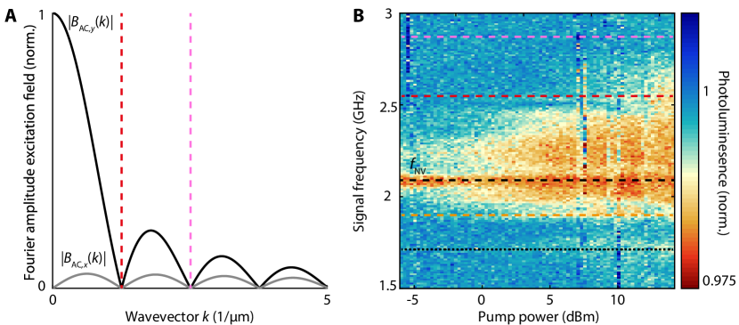
For efficient frequency conversion, the microwaves should excite propagating spin waves with a significant amplitude. The spin-wave excitation efficiency depends on the microwave power and the spatial mode overlap between the drive field and the spin waves [33]. In our experiment, a 5-micron-wide stripline creates an inhomogeneous microwave drive field with a sinc-like amplitude in -space (Fig. S1A). The efficiency drops with decreasing wavelength with nodes at , where is the stripline width and is an integer.
To characterize the dependence on the drive field, we measure the bandwidth induced by four-wave mixing as a function of the pump power (Fig. S1B). As expected, the bandwidth increases with microwave power. The photoluminescence contrast is suppressed at spin-wave frequencies that correspond to the nodes of the drive field in Fig. S1A (colored dashed lines). The frequencies of these modes agree with the spin-wave dispersion derived in the previous section [Eq. (S10)]. The spin-wave excitation antenna is therefore an important design parameter for hybrid diamond-magnet microwave sensors.
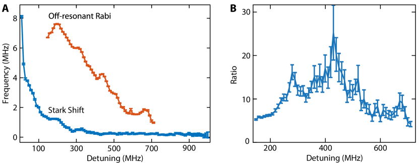
S3. Comparison between the idler-driven Rabi frequency and dynamical Stark shift
A strong microwave field detuned by from the NV ESR frequency (), causes the latter to shift, an effect known as the AC (or dynamical) Stark shift [34]. The Stark shift increases with drive power and is inversely proportional to , which allows detecting the presence of an off-resonant microwave signal. We show here that the idler-driven Rabi frequency resulting from four-spin-wave mixing is about an order magnitude larger than the Stark shift at the same off-resonant drive power.
We measure the Stark shift via pump-probe microwave spectroscopy. The high-power pump is detuned from by 10-1000 MHz, while a low-power probe measures the ESR frequency. We determine the Stark shift for every detuning by measuring the ESR frequency with and without pump (blue data in Fig. S4A).
Next, we measure Rabi oscillations using the four-spin-wave mixing technique. We extract the Rabi frequency for signal spin waves detuned from 10 to 710 MHz (red data in Fig. S4A). We attribute the small oscillations in the Rabi frequency and Stark shift to frequency-dependent (cable) resonances in the microwave transmission of the stripline. Fig. S4B shows that the Rabi frequencies are larger than the Stark shift by about an order of magnitude over the measurement range.
S4. Eight-modes model
Here we describe the details of the model for the spin-wave dynamics under a two-tone drive used to calculate the idler amplitude as a function of pump and signal power, as plotted in Fig. 3E in the main text.
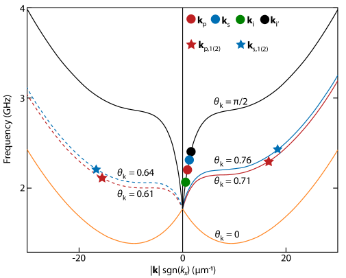
Fig. S5 shows the spin-wave dispersion of a YIG film for (blue line) and (black line), where is the angle between the in-plane spin-wave wavevector and the static magnetization for the parameters in Table S1. Since the out-of-plane component of the applied bias field is small compared to the demagnetizing field of 178 mT in YIG, we assume that the static magnetization lies in-plane along ( is the out-of-plane axis), parallel to , the in-plane component of . The long stripline along excites signal and pump spin waves with . Conservation of momentum dictates that the two created idler spin waves also lie on the branch with wavevectors and (Fig. S5).
When the pump mode is strongly driven beyond a certain threshold, the four magnon scattering term in the spin-wave Hamiltonian leads to a Suhl instability. Here is the annihilation (creation) operator for a magnon with wavevector , which is normalized by , where is the total number of spins, is the volume, is the number of spins per unit cell, and is the unit cell volume. A specific pair of magnons wins the “instability competition”, and , which we call the “efficient Suhl pair” of the pump mode. The efficient Suhl pair for the signal and should also be considered when its mode amplitude is sufficiently large. We disregard cascades that lead to the weak higher-order idlers in Fig. 2F of the main text, as well as the Suhl pairs of the idlers that are safely below their instability threshold at the presently applied powers. A minimal model should therefore include the eight modes indicated in Fig. S5.
The efficient pump and signal pairs can be identified from the threshold amplitude of the pump (signal) mode above which the Suhl instability leads to pairs, which solve [35]
| (S11) |
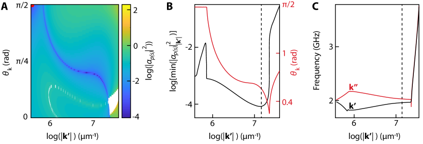
where , with an angular frequency, and is a dissipation rate chosen here to be 10 MHz for all modes. () is the matrix element for the scattering process () in the Hamiltonian [36]. First, we numerically calculate the threshold amplitude as a function of and as in Fig. S6A. We identify the minimum threshold amplitude in the (,) plane of Fig. S6A as a function of modulus in Fig. S6B. The corresponding and spin-wave pair frequencies are shown in Figs. S6B and S6C, respectively. The spin-wave pair with the lowest threshold amplitude – the effective pump (signal) Suhl pair – turns out to be at angles far from (as indicated by the vertical dashed lines in Fig. S6B-C).
Our model Hamiltonian reads
| (S12) |
Here , and “H.c.” denotes the Hermitian conjugate. and are the drive amplitudes of the signal and pump modes, respectively, which are related to the excitation power of the microstrip by (cf. Fig. S1A),
| (S13) |
Here, is the vacuum permeability, is the thickness of the stripline and is its width, is the impedance at , and we assumed . We adopt , nm, m, , where is the length of the excited part of the sample, , and , corresponding to . From the four-magnon-scattering parameters , and , and , and we calculate the mean field amplitude of the idler mode as a function of and . In Fig. 3E of the main text we plot , since it is linearly proportional to the idler-driven Rabi frequency of the NV center [33].
We find an idler amplitude (and thus a Rabi frequency) that initially grows as a function of pump and signal power. However, above the Suhl instability thresholds, the amplitude of the idler mode decreases due to the newly opened dissipation channels, as observed in the experiments in Fig. 3D of the main text. Since , can be scaled by to achieve the same phase diagram for shifted by dBm. Our current assumption of MHz for corresponds to a Gilbert damping of .
S5. Difference-frequency generation by the longitudinal component of the magnetization
In this section we demonstrate that simultaneous transverse magnetization dynamics at the signal and pump frequencies ( and , respectively) causes a beating in the longitudinal component at the difference frequency . The normalized transverse magnetization of two propagating circularly-polarized spin waves is the superposition
| (S14) |
is the wavevector of the th spin wave, with , in terms of the wavelength , is the angular frequency and is the magnetization amplitude normalized by the saturation magnetization. The transverse and components are the real and imaginary parts of while the normalized longitudinal component of the magnetization reads
| (S15) |
When driving two spin waves at frequencies and , and amplitudes and , the squared modulus
| (S16) |
depends on time. For the longitudinal component oscillates at the difference frequency
| (S17) |
as detected in our experiments.
| Material | (A/m) | (J/m) | (J/m3) | Reference |
|---|---|---|---|---|
| YIG | Ref. [33] | |||
| Permalloy (Py) | ||||
| Cobalt (Co) | ||||
| CrBr3 | Ref. [37] | |||
| CrI3 | Ref. [37] | |||
| Fe3GeTe2 | Ref. [38] |